


Introduction
As habitat loss has caused species’ distributions to contract, protected areas (PAs) play an increasingly important role in protecting mammal populations (Pacifici et al. Reference Pacifici, Di Marco and Watson2020). Ongoing land-use change places increasing emphasis on the need for PAs to be effective conservation measures (Geldmann et al. Reference Geldmann, Manica, Burgess, Coad and Balmford2019).
Measures of the representation of species within PAs are based on the estimated overlap of species’ geographical distributions and PA boundaries (e.g., Gray et al. Reference Gray, Hill, Newbold, Hudson, Börger and Contu2016, Maxwell et al. Reference Maxwell, Cazalis, Dudley, Hoffmann, Rodrigues and Stolton2020). This approach does not consider whether PAs contain sufficient suitable habitat to support populations large enough to be considered viable (i.e., self-sustaining despite fluctuations due to stochasticity; Hilbers et al. Reference Hilbers, Santini, Visconti, Schipper, Pinto, Rondinini and Huijbregts2017) and the need to effectively manage threats to species that might compromise population persistence (Geldmann et al. Reference Geldmann, Barnes, Coad, Craigie, Hockings and Burgess2013).
PAs should be large enough to support viable populations due to many occurring in landscapes surrounded by incompatible land uses (Cook et al. Reference Cook, Valkan and McGeoch2019). Where PAs exist in fragmented and disturbed landscapes, they must often function alone to support populations because metapopulation dynamics become challenging to maintain, leaving some species exposed to extinction risk (Kun et al. Reference Kun, Oborny and Dieckmann2009). Such populations may persist for a time but will ultimately be lost (Woodroffe & Ginsberg Reference Woodroffe and Ginsberg1998).
Assessing the capacity of PAs to support populations over time requires an estimate of the minimum number of individuals needed to ensure that that population is resilient to natural fluctuations (i.e., a minimum viable population (MVP) size). Hilbers et al. (Reference Hilbers, Santini, Visconti, Schipper, Pinto, Rondinini and Huijbregts2017) developed an approach to approximate MVP size for a wide range of mammal species, drawing on identified allometric relationships between body mass and life-history characteristics. Their approach also accounts for the impact of environmental conditions on population growth rates (Hilbers et al. Reference Hilbers, Schipper, Hendriks, Verones, Pereira and Huijbregts2016). These MVP estimates have been used to consider the likely minimum area required to support viable populations (minimum viable area; MVA) by incorporating the estimated population density for a species (Santini et al. Reference Santini, Di Marco, Boitani, Maiorano and Rondinini2014, Clements et al. Reference Clements, Kearney and Cook2018a). This framework offers the potential to consider the contribution PAs could make to supporting species persistence for portfolios both of species and of PAs (Clements et al. Reference Clements, Kearney and Cook2018a).
With PAs being the primary tool for species conservation, there have been growing calls for a clearer understanding of the role these areas play in ensuring the persistence of mammal species (Pacifici et al. Reference Pacifici, Di Marco and Watson2020). Santini et al. (Reference Santini, Di Marco, Boitani, Maiorano and Rondinini2014) considered the contribution of PAs to MVPs at a landscape scale, making the important assumption that species can move through the matrix to reach habitat patches outside PAs. However, with many PAs being small (Cook et al. Reference Cook, Valkan and McGeoch2019) and isolated (Saura et al. Reference Saura, Bertzky, Bastin, Battistella, Mandrici and Dubois2018), understanding the current standalone capacity of PAs to support species is a critical element of ensuring PA networks are effective into the future.
Supporting viable populations on private land
Studies that consider the capacity of PAs to support species persistence are largely focused on public PA networks, yet there is interest in understanding the contribution of the growing number of PAs on private land (Stolton et al. Reference Stolton, Redford and Dudley2014, Bingham et al. Reference Bingham, Fitzsimons, Redford, Mitchell, Bezaury-Creel and Cumming2017, Clements et al. Reference Clements, Kerley, Cumming, De Vos and Cook2019). Privately protected areas (PPAs) are parcels of land under private governance that meet the definition of PAs – having the primary objective of biodiversity conservation with a legal mechanism for long-term protection (Stolton et al. Reference Stolton, Redford and Dudley2014). Studies that explore the role of PPAs in strengthening PA networks have primarily focused on biodiversity representation (e.g., Gallo et al. Reference Gallo, Pasquini, Reyers and Cowling2009, Shanee et al. Reference Shanee, Shanee, Monteferri, Allgas, Pardo and Horwich2017, Schutz Reference Schutz2018, Ivanova & Cook Reference Ivanova and Cook2020). In some contexts, PPAs complement the rest of the PA network, protecting poorly represented species (e.g., South Africa, Gallo et al. Reference Gallo, Pasquini, Reyers and Cowling2009, Clements et al. Reference Clements, Kerley, Cumming, De Vos and Cook2019). In other contexts, PPAs have strong overlap with public PAs in the biodiversity represented (e.g., Peru, Shanee et al. Reference Shanee, Shanee, Monteferri, Allgas, Pardo and Horwich2017; Chile, Schutz Reference Schutz2018; Australia, Ivanova & Cook Reference Ivanova and Cook2020). Yet little is known about the contributions PPAs make to supporting viable populations, leaving a critical gap in our understanding of the role these areas play in building robust PA networks.
From representation to long-term persistence
Given the need to better understand the potential of PAs to support species persistence, we sought to analyse which PAs are likely to support viable populations of species within the context of a large national PA network: Australia. We also sought to understand the contribution PPAs make to supporting viable populations of species given that they form a prominent and growing part of the broader PA network (Ivanova & Cook Reference Ivanova and Cook2020). Lastly, we aimed to identify the species for which the PA network is estimated to provide adequate support and those species that remain vulnerable. Based on this analysis, we highlight opportunities to strengthen the PA network into the future.
Methods
Study system
Australia is one of the world’s mega-diverse nations (Mittermeier et al. Reference Mittermeier, Gil and Mittermeier1997) and at the same time a global epicentre for species extinction (Woinarski et al. Reference Woinarski, Burbidge and Harrison2015), where many species continue to decline (Woinarski et al. Reference Woinarski, Burbidge and Harrison2014, Garnett & Baker Reference Garnett and Baker2021). Understanding how PAs support species long-term may help better direct future conservation efforts.
The Australian PA network occupies c. 20% of the country’s landmass (Fig. S3.1), including a growing number of PPAs that currently account for 6.6% of this area protected (Ivanova & Cook Reference Ivanova and Cook2020). In Australia, PPAs are highly secure, legally binding, in-perpetuity agreements (Hardy et al. Reference Hardy, Fitzsimons, Bekessy and Gordon2017), giving them the same status as other PAs (e.g., state-owned and Indigenous PAs, hereafter ‘public PAs’). We sought to consider whether the large number of PAs and substantial area under protection translate into a robust network that supports species persistence.
Habitat model development
To identify suitable habitat for species within Australia’s PA network, we constructed detailed habitat models for 118 Australian mammal species (Fig. 1) with the necessary data available, approximately a third of Australia’s estimated 386 extant native mammals (Chapman Reference Chapman2009).

Fig. 1. The process used to determine the potential of protected areas (PAs) to support viable populations of 118 species across all PAs in the Australian PA network. HFI = Human Footprint Index (Venter et al. Reference Venter, Sanderson, Magrach, Allan, Beher and Jones2018); IUCN = International Union for Conservation of Nature; MVP = minimum viable population size (Hilbers et al. Reference Hilbers, Santini, Visconti, Schipper, Pinto, Rondinini and Huijbregts2017); MVA = minimum viable area required to support an MVP (Clements et al. Reference Clements, Kearney and Cook2018a).
The habitat models were developed based on literature-sourced habitat descriptions (Table S1.3), which we matched with vegetation subgroups from Australia’s National Vegetation Information System (Table S1.3). We validated the selection using the Atlas of Living Australia (ALA) species occurrence records (https://biocache.ala.org.au/occurrences; Table S1.1). In some cases, occurrence records led to additional vegetation subgroups being included in the habitat models (Appendix S1). Each species’ habitat model was further refined using information noted in the habitat descriptions about rainfall, altitude and/or any association with rocky outcrops (e.g., Petrogale assimilis; Table S1.3). No other environmental parameters were consistently mentioned as distinguishing features in the habitat descriptions.
To apply the habitat models, we used the species’ distributions from the International Union for Conservation of Nature (IUCN) Red List database (version 2019_3; https://www.iucnredlist.org). We restricted these distributions to areas of overlap with the habitat models developed (Fig. 1) and introduced a buffer equal to the dispersal distance of the species to account for potential species’ usage of the adjoining areas (Table S2.3). Our process of using suitable habitat descriptions to refine species’ distributions provides a more accurate reflection of where species are likely to occur across the landscape (Cantú-Salazar & Gaston Reference Cantú-Salazar and Gaston2013) relative to studies that use the coarse distributions (e.g., Rondinini et al. Reference Rondinini, Di Marco, Chiozza, Santulli, Baisero and Visconti2011, Santini et al. Reference Santini, Di Marco, Boitani, Maiorano and Rondinini2014, Clements et al. Reference Clements, Kearney and Cook2018a). When validated using species occurrence records from the ALA, we achieved an average of 84.9% (±2.1 SE) agreement with our habitat models (Appendix S1).
We clipped the edited distributions for each species to PA boundaries to identify PAs that support the species’ habitat (Fig. 1). The PA boundaries for Australia were identified using spatial data from the Collaborative Australian Protected Areas Database (CAPAD). We updated this database to resolve the well-acknowledged spatial inconsistencies in PA boundaries (e.g., poorly drawn and overlapping polygons; Cook et al. Reference Cook, Valkan, Mascia and McGeoch2017) and to supplement the incomplete records of PPAs (Clements et al. Reference Clements, Selinske, Archibald, Cooke, Fitzsimons and Groce2018b, Archibald et al. Reference Archibald, Barnes, Tulloch, Fitzsimons, Morrison, Mills and Rhodes2020). See Appendix S1 and Ivanova & Cook (Reference Ivanova and Cook2020) for details.
Determining the area required to support populations over the long term
We defined viable areas of habitat as those large enough to support a viable population, where population viability is a 95% probability of persistence over 100 years, despite environmental and demographic stochasticity (as per Clements et al. Reference Clements, Kearney and Cook2018a). We sourced estimates of MVP sizes from Hilbers et al. (Reference Hilbers, Santini, Visconti, Schipper, Pinto, Rondinini and Huijbregts2017), as they found their MVP estimates to be robust when validated against species- and/or context-specific studies, with the targets falling within the same order of magnitude. This approach aligns with evidence that body mass is a reliable predictor of habitat area requirements for small to medium-sized mammals (<10 kg; Noonan et al. Reference Noonan, Fleming, Tucker, Kays, Harrison and Crofoot2020), covering the majority of Australian mammals and those most prone to extinction (Johnson & Isaac Reference Johnson and Isaac2009).
We calculated the area of habitat required by each species to support a viable population (MVA) by dividing the MVP size for each species by its estimated average population density (Fig. 1). We obtained population density estimates for 90 species from Clements et al. (Reference Clements, Kearney and Cook2018a) and sourced estimates for a further 28 species from the literature (Table S1.2).
Hilbers et al. (Reference Hilbers, Santini, Visconti, Schipper, Pinto, Rondinini and Huijbregts2017) provide a mechanism to adjust estimated MVP sizes according to environmental conditions by penalizing the intrinsic rate of growth in their models (Hilbers et al. Reference Hilbers, Schipper, Hendriks, Verones, Pereira and Huijbregts2016), such that poorer habitat quality requires a larger population size to be viable. Habitat quality is composed of a complex set of parameters and is highly species- and context-specific, in addition to there being inevitable inconsistencies in the use of the term (Johnson Reference Johnson2007). We chose to use the Human Footprint Index (HFI; Venter et al. Reference Venter, Sanderson, Magrach, Allan, Beher and Jones2018) as a proxy of human pressures to give an indication of habitat quality, as this is a commonly used dataset available at the scale required for this study. The HFI provides a measure of eight anthropogenic pressures that impact on habitat quality (e.g., human population density, roads, night-time lights), creating a continuous scale (0–50) at a 1km2 resolution. We calculated the mean HFI score for each PA (Fig. 1 & Appendix S1). Hilbers et al. (Reference Hilbers, Santini, Visconti, Schipper, Pinto, Rondinini and Huijbregts2017) provide MVP estimates for six different levels of habitat quality, so accordingly we grouped the continuous HFI scores into six categories to represent very poor habitat quality to ideal habitat (Table S1.4).
We determined that a PA had the capacity to independently support a viable population if it contained suitable habitat of a sufficient size (MVA) to support an MVP, after accounting for the impact of habitat quality (i.e., HFI score) on the size of the population (Fig. 1). We calculated the number of MVPs that could be supported by the suitable habitat within each PA for each species independently.
Identifying which PAs support viable populations
For each species, we used the estimated number of MVPs in each PA to identify which PAs could independently support at least one viable population (i.e., ≥1 MVP; Fig. 1) and whether these were PPAs or public PAs.
To investigate patterns in how well different species are supported by the PA network as a whole, we used a K-means cluster analysis to group species according to: (1) the proportion of relevant PAs that could support at least one MVP of the species; and (2) the proportion of those PAs that were privately managed (PPAs). We followed the Elbow method (Syakur et al. Reference Syakur, Khotimah, Rochman and Satoto2018) in determining the most fitting number of clusters for the data (Fig. S1.2). The cluster analysis identified groups of species facing different situations, from those with many PAs contributing potentially viable populations, to those with many PAs not able to support a single viable population of the species, separated according to the level of contribution made to protecting viable populations by PPAs. We then evaluated factors that might account for some of these patterns across species, such as body mass, total available habitat area and taxonomic group.
We explored the impact of habitat quality and the amount of habitat contained within PAs on the probability that a PA could support an MVP. For each species, we used a two-sample t-test to compare the mean HFI score of PAs that were estimated to support at least one MVP versus those that were not. We assessed this separately for public PAs and for PPAs. To allow for an assessment of the relationship between habitat area and the probability of a PA supporting an MVP, given the large sample size, we divided PAs into three groups according to the area of a species’ habitat they contained (<1 km2, 1–5 km2 and >5 km2) and examined how many in each group support at least one MVP (Appendix S1). We compared the habitat area groupings separately for public PAs and PPAs to identify any difference in outcome that may be due to land tenure type.
Are enough PAs supporting viable populations?
Species that are rare or have had their distribution severely diminished are typically considered in need of additional protection (Pimm et al. Reference Pimm, Jenkins, Abell, Brooks, Gittleman and Joppa2014). Recognizing this, the outcome for each species was further assessed based on the percentage of relevant PAs that could support an MVP. To do this, we created a ’protection threshold’ – the minimum level of protection that should be offered to species by the PA network. The protection threshold is measured by the percentage of PAs with suitable habitat that need to support at least one viable population of that species. This threshold is based on the distribution of the species, with a protection threshold of 100% of relevant PAs for species with <1000 km2 of habitat available through to 10% coverage for species with >10 000 km2 of habitat available. The percentage is linearly interpolated for species with habitat areas between 1000 and 10 000 km2 (Clements et al. Reference Clements, Kearney and Cook2018a).
While our analysis explored whether PAs have sufficient habitat to support an MVP, threats to species play an important role in determining population persistence. Species within the critical weight range (CWR) of 35–5500 g are highly susceptible to predation by introduced foxes (Vulpes vulpes) and feral cats (Felis catus; Key Threatening Processes under the Environment Protection and Biodiversity Conservation Act 1999). Thus, we used the CWR as an indicator of species where habitat protection alone is unlikely to ensure persistence of a species in the absence of predator control. This mattered most where PAs did not meet the protection threshold for a species, as those species cannot rely on PAs (i.e., spaces most favourable to invasive species control) and require additional resources to secure long-term protection. In discussing species management options, we also considered the IUCN Red List threat status of the species and formally listed key threats.
All spatial analyses were carried out in ArcGIS Pro version 2.3 (ESRI 2019). K-means cluster analysis was performed in SPSS Statistics 27 (IBM Corp. 2020).
Results
We found that the Australian PA network has the potential to support viable populations (≥1 MVP) for all 118 of the mammal species studied and that PPAs can support viable populations for 107 of those species (Table S2.1). In principle, this means that Australian PAs include enough habitat to sustain all of our study species in at least a few sites over the long term without relying on the surrounding matrix. PPAs contribute to this result for 91% of species despite only accounting for 6.6% of PAs by area.
Patterns of species protection within the PA network
While the existing PA network can potentially support viably sized populations of all study species, not all PAs that overlapped a species’ habitat were large enough to support a viable population (<1 MVP). We found that species belonged to one of four key groups in this respect (Fig. 2).
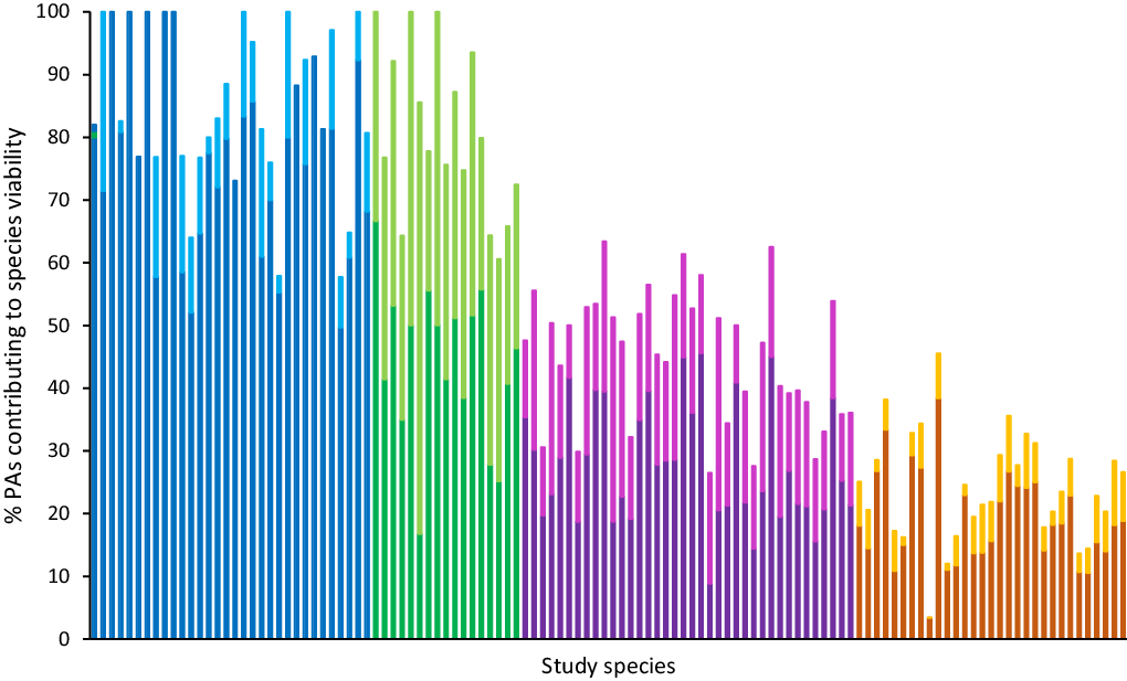
Fig. 2. The percentage of protected areas (PAs) containing suitable habitat for species that also support at least one viable population of that species, presented for the study species (n = 118, ordered alphabetically for each group). Each bar denotes a species, with the darker shade representing the proportion of public PAs and the lighter shade representing the proportion of privately protected areas making up the total percentage. The colours represent the four groups identified by the K-means cluster analysis (from left to right: blue = Group 1; green = Group 2; purple = Group 3; orange = Group 4).
Groups 1 and 2 (42% of species) were dominated by species where most PAs contained sufficient habitat to support one or more viable population. These species were either principally present in public PAs (Group 1, n = 32; blue in Fig. 2) or distributed equally across public PAs and PPAs (Group 2, n = 17; green in Fig. 2). Group 1 largely represented species from the Dasyuridae and Muridae families, while Group 2 was dominated by Macropodidae and Pseudocheiridae (Fig. 3). Species in Group 2 tended to be larger bodied than those in Group 1 (Fig. S3.3B) but occupied much narrower distributions (Table S2.3).

Fig. 3. Attributes of the four key groups of species identified based on the contribution that protected areas (PAs) make to supporting viable populations (Fig. 2; group colours match). Each panel shows the most distinguishing mammalian families, the range of body masses and the median range size for species (represented by the magnifying glass over the Australian continent) for species within the group. The pie charts demonstrate the proportion of PAs that are (‘Viable PAs’) and are not (‘Non-viable PAs’) able to support viable populations (larger pie charts) and the proportion of viable PAs that are on public (‘Public PAs’) and private (‘PPAs’) land tenure (smaller pie charts). Note: the magnifying glasses are indicative of the relative geographical range size but do not show the geographical location of the species. Symbols courtesy of the National Environmental Science Program (NESP) Resilient Landscapes Hub (www.nesplandscapes.edu.au). PPA = privately protected area.
For most species in Groups 3 and 4, the majority of PAs did not support viable populations (<1 MVP; 58% of study species). PPAs tended to make up a greater proportion of the PAs with viably sized habitat for Group 3 (n = 38; purple in Fig. 2) than they did for Group 4 (n = 31; orange in Fig. 2). Groups 3 and 4 were composed of a diverse range of mammalian families (Figs 3 & S3.2) – Group 3 included many species from the Phalangeridae, Macropodidae and Muridae families, while for Group 4 species were largely Dasyuridae, Petauridae and Potoroidae. Similarly to Group 1, Group 4 species tended towards smaller body sizes (Fig. S3.3B), while Group 3 species were larger bodied. Species in Groups 3 and 4 were similar in terms of having very large distributions, approximately double those of species in Group 1 (Fig. 3) and almost 20 times larger than those of species in Group 2.
How many PAs contribute to the long-term viability of species?
Twenty-six species were estimated to have no more than 20 PAs supporting MVPs. Thirteen of those were in Group 1, where most of the available PAs did support MVPs but few PAs contained suitable habitat (Table S2.1). Within Groups 3 and 4, where most PAs with suitable habitat were not large enough to support a viable population, there were nine species with 20 or fewer PAs able to support more than one MVP. In contrast to similar species in Group 1, they had many more PAs with suitable habitat.
Factors contributing to the ability of PAs to support MVPs
We found that habitat area and quality appeared to drive some of the patterns when PAs were not able to support a viable population (<1 MVP). Across all PAs, the mean HFI score represented very good habitat quality (0.9 out of 1.0) for both public PAs and PPAs (Table S2.3). PAs with higher-quality habitat can support higher population densities, and we found that PAs that can support at least one MVP had significantly higher habitat quality across both public PAs (t = 1.98, df = 135, p < 0.001) and PPAs (t = 1.98, df = 129, p < 0.001). Similarly, species belonging to Groups 1 and 2 were found in PAs with superior habitat quality to those in Groups 3 and 4 (Fig. 4), where most PAs did not support ≥1 MVP (Fig. 2).

Fig. 4. The proportion of protected areas (PAs) falling within each of the six habitat quality categories formulated using the Human Footprint Index (ranging from 0 representing very-poor-quality habitat to 1 representing ideal habitat) for the species studied (n = 118, ordered alphabetically for each group). Each bar represents a species, with species presented in the four groups identified in Fig. 2 (groups are separated by black bars).
Beyond habitat quality, many PAs were unable to support MVPs due to constraints on the area of suitable habitat available. When less than 1 km2 of habitat was available within a PA, only 16% were able to support an MVP (Fig. S3.4). This is a particularly big challenge for PPAs, where c. 63% contained blocks of habitat smaller than 1 km2 (Table S2.2). Habitat patch size was the most prominent difference between PPAs and public PAs. Public PAs were more likely to contain blocks of habitat greater than 5 km2 in size (53% of public PAs; Table S2.2), and once over this threshold, almost all PAs could sustain ≥1 MVPs (95% for public PAs, 96% for PPAs). Poor habitat quality compounded the challenge for PAs with smaller habitat patches to support an MVP (Fig. S3.5).
PAs meeting species’ protection thresholds
According to the protection threshold we defined, as many as 92 species had >10 000 km2 of suitable habitat and therefore could meet the threshold, with PAs supporting viable populations (≥1 MVP) across only 10% of this habitat. In contrast, six species had <1000 km2 of suitable habitat available, and therefore meeting the threshold required 100% of this habitat to be contained within viable PAs. We found that for 86 of the 118 species, the Australian PA network was able to meet the protection threshold we set (Fig. 5 & Table S2.3). Importantly, 59% (n = 51) of these 86 species were within the CWR (Table S2.3). Thirteen species are categorized as threatened on the IUCN Red List, and invasive predators are a key threat for 12 of these species (Table S2.4).

Fig. 5. The outcome for each species relative to the set protection threshold, defined based on the size of species habitat (orange dashed line marks the point along the orange left-hand y-axis where the threshold is reached), as achieved by the Australian protected area (PA) network. The percentages of species habitat contained within privately protected areas (PPAs) that support at least one viable population are marked in blue along the right-hand y-axis.
A further nine species did not have sufficient habitat within PAs that can support viable populations (≥1 MVP), with their PAs falling short of our target for protection by <10%. The remaining 23 species fell well below the threshold and would require a significant investment in additional PAs and/or habitat restoration to reach the protection target (Fig. 5). In many cases, the majority of remaining habitat for these species occurs on private land (Table S2.3), underlining the importance of expanding the network to include more PPAs. The 32 species that fell below the protection threshold were mostly within the CWR (n = 22). A third (n = 11) of those are threatened species, citing cat and/or fox predation as key drivers of their declines (Table S2.4).
At only 6.6% of the total Australian PA network, PPAs did not change the outcome of whether the protection threshold was met for any of our study species. However, despite their small area, PPAs often performed far above expectations, protecting >27% of habitat within viably sized PAs (≥1 MVP) for seven species (Fig. 5). Six of these seven species are categorized as threatened, highlighting the critical role PPAs play in supporting their conservation.
Discussion
Australia’s PA network appears to be largely well-designed for the conservation of mammals in this study. This was true for species with large and small habitat requirements and for widespread and narrowly distributed species. However, given the range of pressures on biodiversity, supporting the long-term persistence of mammals requires more than protecting a single viable population.
Supporting long-term persistence by spreading risk
Considering the proportion of PAs able to support MVPs of species in their own right helps us to understand the probability that species are buffered against stochastic factors, minimizing their extinction risk (Ovaskainen Reference Ovaskainen2002, McCarthy et al. Reference McCarthy, Thompson, Moore and Possingham2011). In total, 58% of our study species largely occur in PAs estimated not to be large enough to support a viable population (Fig. 2). Those PAs are at high risk of suffering an extinction debt over the medium to long term (Woodroffe & Ginsberg Reference Woodroffe and Ginsberg1998), particularly where the assumption of viable metapopulations across small, isolated habitat patches (e.g., Santini et al. Reference Santini, Di Marco, Boitani, Maiorano and Rondinini2014) does not hold, such as in fragmented landscapes.
More than a fifth of species studied were supported in 20 or fewer PAs of sufficient size. Species concentrated in only a few sites are more vulnerable to extinction (Brown et al. Reference Brown, Bolger and Fennessy2019), which in our study principally concerns species in Groups 1 and 2. PAs do support viable populations of these groups; however, their species are only found across a small number of PAs, often because they have suffered significant habitat loss, as is the case for Lagostrophus fasciatus (Group 2), or they have a naturally restricted distribution, such as Pseudochirulus cinereus (Group 1). As such, most suitable habitat is already protected and little opportunity exists to increase the number of PAs – a critical consideration given that the risk of catastrophic events is set to increase with climate change (Canadell et al. Reference Canadell, Meyer, Cook, Dowdy, Briggs and Knauer2021). For example, wildfires in Australia are projected to become more frequent (Bowman et al. Reference Bowman, Williamson, Yebra, Lizundia-Loiola, Pettinari and Shah2020), which is devastating for wildlife given the scale of resultant destruction (e.g., millions of hectares of habitat lost in the 2019/2020 summer season). Even small amounts of habitat loss or degradation can be significant to range-restricted species (Staude et al. Reference Staude, Navarro and Pereira2020), so insurance populations or ex situ conservation initiatives may be necessary (Pritchard & Harrop Reference Pritchard and Harrop2010).
We found that PPAs make critical contributions to spreading the extinction risk particularly for the larger-bodied species in Groups 2 and 3 (Figs 3 & S3.3A), and this contribution was often due to the positioning of private land. Private land tends to be arable (Gallo et al. Reference Gallo, Pasquini, Reyers and Cowling2009), so PPAs would probably have richer soils than their public counterparts, and they could help to address some of the long-standing biases in the positioning of PAs (Joppa & Pfaff Reference Joppa and Pfaff2009). While PPAs contribute viable habitat to a diverse range of species (Figs 2–3), the potential of private land is even greater, as identified gaps in species protection coincide with private land more readily than they do with public land (Ivanova & Cook Reference Ivanova and Cook2020).
Improving the capacity of PAs to support persistence
In considering the fraction of their habitat contained within PAs that is likely to support viable populations (the protection threshold), it is encouraging that many species are well-protected across Australia’s PA network (Fig. 5). Nevertheless, 27% of species fell below this threshold, often occurring in small PAs likely to suffer an extinction debt over the long term (Woodroffe & Ginsberg Reference Woodroffe and Ginsberg1998). The challenges facing small PAs are likely to be the key drivers of outcomes for the long-term persistence of many species. This particularly affects PPAs, which have an average size of 10.3 km2 (±1.5 km2 SE) in Australia (Ivanova & Cook Reference Ivanova and Cook2020). Improving the capacity of PAs to support viable populations is challenging when so many Australian PAs are small (80% less than 10 km2; Cook et al. Reference Cook, Valkan and McGeoch2019) and suitable habitat within them is restricted (45% have <1 km2 of suitable habitat; this study). Nevertheless, as habitat loss and fragmentation continue, smaller PAs become increasingly important for species within heavily cleared habitat. Small PAs would enhance the connectivity that is critical to species persistence (van Teeffelen et al. Reference van Teeffelen, Cabeza and Moilanen2006). Australia lags behind many other countries in connectivity measures (Saura et al. Reference Saura, Bertzky, Bastin, Battistella, Mandrici and Dubois2018); therefore, this requires a greater focus within Australia’s PA network, especially under climate change (Thornton et al. Reference Thornton, Branch and Murray2020).
Habitat size and habitat quality are both important parameters within MVP calculations (Hilbers et al. Reference Hilbers, Schipper, Hendriks, Verones, Pereira and Huijbregts2016), and both affect whether or not a PA is likely to support a viable population (Fig. S3.5). Given that the habitat area within PAs cannot be increased in many cases, increasing the carrying capacity of habitat could be one approach to reducing the extinction risk for some threatened species (Di Minin et al. Reference Di Minin, Hunter, Balme, Smith, Goodman and Slotow2013). We found that habitat quality was an important predictor of whether PAs were likely to support viable populations of species (Fig. 4). Therefore, habitat management could partly compensate for the small size of many PAs.
It is important to acknowledge that the proxy we selected for habitat quality in this study (the HFI) is an imperfect measure of habitat condition. While it considers multiple stressors, the biological effects of which are well-documented (e.g., light pollution effects; Gaston et al. Reference Gaston, Bennie, Davies and Hopkins2013), and it is a widely used proxy for anthropogenic threats, the HFI provides only a coarse measure of habitat quality, especially for small PAs (i.e., the spatial scale of 1km2 grids exceeds the size of many small PAs). Many of the species included in our study are vulnerable to other threatening processes within PAs that also impact habitat quality, such as invasive predators. These pressures would also need to be managed in PAs theoretically large enough to support viable populations in order to ensure population persistence.
The role of PPAs in supporting species persistence
While PPAs in Australia represent many of the same species as public PAs do (Ivanova & Cook Reference Ivanova and Cook2020), we found that they tend to make only a small contribution to supporting viable populations relative to public PAs (Fig. 5). Despite this, PPAs are important in supporting several species that fall below the desired protection threshold (i.e., where only a small proportion of their habitat is contained within viably sized PAs; Fig. 5). Importantly, most of these species are categorized as threatened and have very narrow habitat ranges, such as Myrmecobius fasciatus, which is specifically targeted for conservation by PPAs (Australian Wildlife Conservancy 2019). Of the 10 species for which PPAs make the largest contribution towards protecting viable habitat, eight have the majority of their habitat on private land (Table S2.3). As such, some species have a very high reliance on PPAs that may not be otherwise met by other PA governance types (Kareiva et al. Reference Kareiva, Bailey, Brown, Dinkins, Sauls and Todia2021).
Can long-term persistence be guaranteed by viably sized PAs?
Long-term persistence of species in PAs extends beyond sufficient habitat area – recognizing and dealing with threatening processes are critical actions when assessing the efficacy of PAs (Gaston et al. Reference Gaston, Pressey and Margules2002) and their surrounding buffer areas (Hansen et al. Reference Hansen, Davis, Piekielek, Gross, Theobald and Goetz2011). In many instances, species persistence will require PAs to be part of an integrated landscape management strategy to mitigate threats (Kearney et al. Reference Kearney, Adams, Fuller, Possingham and Watson2020).
In Australia, landscape-scale disturbances, such as wildfires, introduced predators and herbivores (Woinarski et al. Reference Woinarski, Burbidge and Harrison2015), can be critical in preventing PAs from realizing their potential to support viable populations over the long term. Into the future, dramatic range shifts predicted under climate change will affect the conservation potential of existing PAs (e.g., Ferro et al. Reference Ferro, Lemes, Melo and Loyola2014). Habitat specialists are typically less equipped to tolerate disturbance than habitat generalists (Devictor et al. Reference Devictor, Julliard and Jiguet2008), so specialists should be the principal focus of conservation outlook assessments. For example, Burramys parvus (Group 1) persists in rocky snow-covered alpine regions, while Pseudochirops archeri (Group 2) requires an abundance of trees and vines in its habitat. This nature of species’ habitat requirements in combination with the degree of habitat connectivity will contribute to whether a PA network continues to support viable populations into the future.
Supplementary material
To view supplementary material for this article, please visit https://doi.org/10.1017/S0376892922000455.
Acknowledgements
We thank the many contributors who have made possible the several public databases we used, particularly the Collaborative Australian Protected Areas Database (CAPAD) and the Atlas of Living Australia (ALA). Thank you to H Clements for inspiring the conceptualization of this project and providing some of the population density data used. We would also like to extend our thanks to the two reviewers with whose help the manuscript’s quality has been majorly improved.
Financial support
IMI is supported by the Graduate Research Completion Award provided by Monash University.
Competing interest
The authors declare none.
Ethical standards
None.


 Open access