

INTRODUCTION
Haemorrhagic fever with renal syndrome (HFRS) is a zoonosis caused by Hantaviruses from the family Bunyaviridae. It was first recognized in northeastern China in 1931 and has been prevalent in many other parts of China since 1955. At present, HFRS is endemic in 28 of the 31 provinces of China, autonomous regions, and metropolitan areas and accounts for 90% of HFRS cases reported globally [Reference Luo and Chen1]. HFRS is also endemic in Shenyang, China. HFRS incidence, with an increasing trend, was seen from 1990 to 2003, and reached a historically high level in 2003. A better understanding of the spatial, temporal and space–time distribution patterns of HFRS would help in identifying areas and periods at high risk, and might be very useful in surveillance of HFRS, discovering the risk factors behind its spread, and help better prevent and control HFRS.
Spatial analysis with spatial smoothing and cluster analysis are commonly used to characterize spatial patterns of diseases [Reference Nkhoma2–Reference Odoi6]. A spatial-rate smoother is a special case of a non-parametric rate estimator based on the principle of locally weighted estimation. A map of spatially smoothed rates tends to emphasize broad trends and is useful for identifying general features of the data. The spatial-rate smoother is easy to implement in software systems for exploratory spatial data analysis [Reference Anselin, Lozano and Koschinsky7, Reference Rey and Janikas8].
Scan statistics are used to detect and evaluate clusters in temporal, spatial or space–time settings. Temporal, spatial and space–time scan statistics are now commonly used for disease cluster detection and evaluation, for many diseases including infectious diseases [Reference Cousens9–Reference Fang13], cancer [Reference Kulldorff14–Reference Fukuda17], cardiology [Reference Kuehl and Loffredo18], autoimmune diseases [Reference Donnan19], liver diseases [Reference Ala20], and veterinary medicine [Reference Ward21–Reference Guerin24]. In SaTScan software [Reference Kulldorff25], this is done by gradually scanning a window across time and/or space and noting the number of observed and expected observations inside the window at each location. The scanning window is an interval (in time), a circle or an ellipse (in space) or a cylinder with a circular or elliptic base (in space–time). Multiple different window sizes are used. The window with the maximum likelihood is the most likely cluster, i.e. the cluster least likely to be due to chance; a P value is assigned to this cluster.
The aim of the present study was to investigate the spatial and temporal distribution of confirmed cases of HFRS and identify the areas and periods of high risk. In this study we used the geographical information system and temporal, spatial and space–time scan statistics to investigate statistically significant clusters of HFRS in Shenyang, China during 1990–2003. The tools used in this study provide an opportunity to classify the epidemic situation of HFRS.
METHODS
Data collection and management
The study site is located in Shenyang (122° 25′–123° 48′ E, 41° 11′–43° 02′ N), in the southern part of northeast China and in the central part of Liaoning Province (Fig. 1). The area of Shenyang is 13008 km2, and has a population of 7 200 000. Most of Shenyang region rests on a flat plain. Mountains and highlands are mainly concentrated in the southeastern part, belonging to the extended part of the Liaodong mountainous highlands.
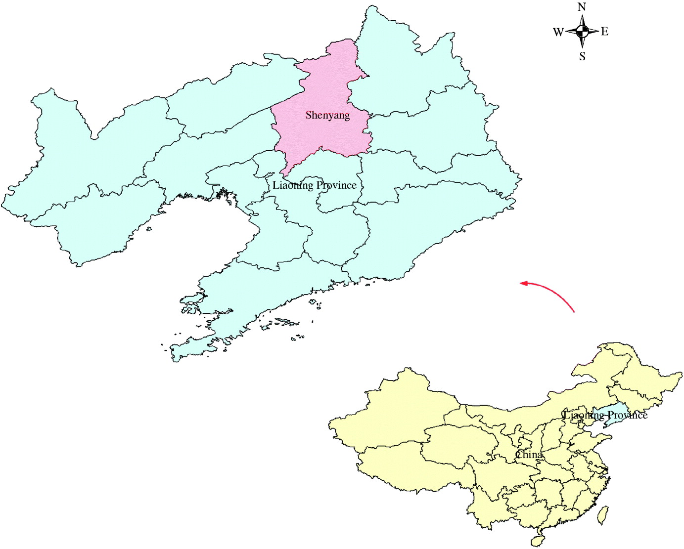
Fig. 1. Location of Shenyang in Liaoning Province, China
There are five urban areas, four suburban areas and four counties in Shenyang. For our study, we used these 13 areas as study areas. The information includes the number of HFRS cases per month and per year in every county from 1990 to 2003. For the 14-year period (1990–2003), the average annual incidence was 3·2 cases/100 000 persons, 3010 cases were involved in this study.
HFRS cases were first diagnosed using clinical symptoms, then blood samples were collected in hospitals, serological identification was performed at the laboratory of Liaoning Provincial Center for Disease Control and Prevention (CDC) to confirm the clinical diagnosis, and the data was collected by case number according to the sampling results. Records on HFRS cases between 1990 and 2003 were obtained from Liaoning Provincial CDC.
To conduct a GIS-based analysis on the spatial distribution of HFRS, a county-level polygon map of Shenyang at a scale of 1:1 000 000 was obtained on which the point layers containing information regarding latitude and longitude of central points of each area were created. Demographic information based on the fifth National Census (2000) was integrated in terms of an administration code. All HFRS cases were geocoded and matched to the county-level layers on the polygons and points by administration code using ArcGIS9.2 software (ESRI Inc., USA).
Thematic maps for the incidence of HFRS
To reduce variations of incidence in small populations and areas, we calculated annualized average incidences of HFRS/100 000 in each area over the 14-year period.
To describe the upper outliers and lower outliers in different areas, a circular cartogram was produced. A circular cartogram is a map where the original irregular polygons are replaced by circles. The placement of the circles is such that the original pattern is mimicked as much as possible, both in terms of absolute location and in terms of relative location (neighbours, or topology). The size (area) of the circles is proportional to the value of the selected variable [Reference Anselin26]. In this study the hinge used to identify outliers was set as 1·5.
Based on annual average incidence, all counties were grouped into three categories: low endemic areas with an annual average incidence between 0 and 2/100 000, medium endemic areas with an incidence between 2 and 5/100 000, and high endemic areas with an incidence >5/100 000. The three types of areas were colour-coded on the maps.
To assess the risk of HFRS in each county, an excess hazard map was produced. The excess risk is the ratio of the observed rate to the average rate computed for all the data. This average is not the average of the county rates. Instead, it is calculated as the ratio of the total sum of all events over the total sum of all populations at risk [Reference Anselin26].
Spatial-rate smoothing consists of computing the rate in a moving window centred on each area in turn. The moving window includes the county as well as its neighbours; the neighbours are defined by means of a spatial weights file. Therefore, the first step in the analysis was to construct a spatial weights file that contained information on the ‘neighbourhood’ structure of each area. The k-nearest-neighbour criterion ensured each observed object had exactly the same number (k) of neighbours. In the analysis, six neighbours were chosen for each county by k-nearest-neighbour criterion. The second step was to load the weights file and perform smoothing analysis [Reference Anselin26].
Spatial autocorrelation analysis
Moran's I spatial autocorrelation statistic and its visualization in the form of a Moran scatter plot are usually used in global spatial autocorrelation analysis. First, a spatial weight was constructed for each area. Second, Moran's scatter plot was produced with a spatial lag of incidence on the vertical axis and a standardized incidence on the horizontal axis. Third, a significant test was performed through the permutation test, and a reference distribution was generated under an assumption that the incidence was randomly distributed. For this study, the number of permutation tests was set to 999 and the pseudo-significance level was set as 0·001.
Spatial, temporal, and space–time cluster analysis
Temporal, spatial, and space–time scan statistics (SaTScan) [Reference Kulldorff25] were applied to identify clusters of HFRS.
The spatial scan statistic imposes a circular window on the map. The window is in turn centred on each of several possible grid points positioned throughout the study region. For each grid point, the radius of the window varies continuously in size from zero to some upper limit specified by the user. In this way, the circular window is flexible both in location and size. In total, the method creates an infinite number of distinct geographical circles with different sets of neighbouring data locations within them. Each circle is a possible candidate cluster of HFRS. In this study, retrospective spatial cluster analysis for higher incidence was used, in which the maximum spatial cluster size was set to be 50% of the total population at risk to find possible sub-clusters.
The space–time scan statistic is defined by a cylindrical window with a circular (or elliptical) geographic base and with height corresponding to time. The base is defined exactly as for the purely spatial scan statistic, while the height reflects the time period of potential clusters. The cylindrical window is then moved in space and time, so that for each possible geographical location and size, it also visits each possible time period. In effect, we obtain an infinite number of overlapping cylinders of different size and shape, jointly covering the entire study region, where each cylinder reflects a possible cluster of HFRS. In the present study, retrospective space–time cluster analysis for higher incidence was used, in which the maximum spatial cluster size was set as 50% of the total population at risk, and the maximum temporal cluster size was set as 50% of the total population at risk in order to find possible sub-clusters.
The temporal scan statistic uses a window that moves in one dimension, i.e. time, defined in the same way as the height of the cylinder used by the space–time scan statistic. This means that it is flexible in both start and end date. In the present study, retrospective temporal cluster analysis for higher incidence was used, in which the maximum temporal cluster size was set as 50% of the total population at risk in order to find possible sub-clusters.
For each window, the method uses a Monte Carlo simulation to test the null hypothesis that there is not an elevated risk of HFRS. Details of how the likelihood function is maximized over all windows under the Poisson assumption have been described in SaTScan [25]. For each window of movable position and size change, the software tested the risk of HFRS within and outside the window using the null hypothesis of the same risk.
RESULTS
Spatial distribution of HFRS in Shenyang
There were a total of 3010 HFRS cases reported in Shenyang, from 1990 to 2003. The annual average incidence ranged from 0·10 to 10·18/100 000.
The cartogram uses size (area) and colour code to provide additional information about specific values, such as negative values, zero and outliers. The default colour is green. Zeros are shown as transparent, upper outliers as red, and lower outliers as blue. In our study, when the hinge used to identify outliers was set to be 1·5, one area was recognized as an upper outlier, and there were no zero and lower outlier (Fig. 2).
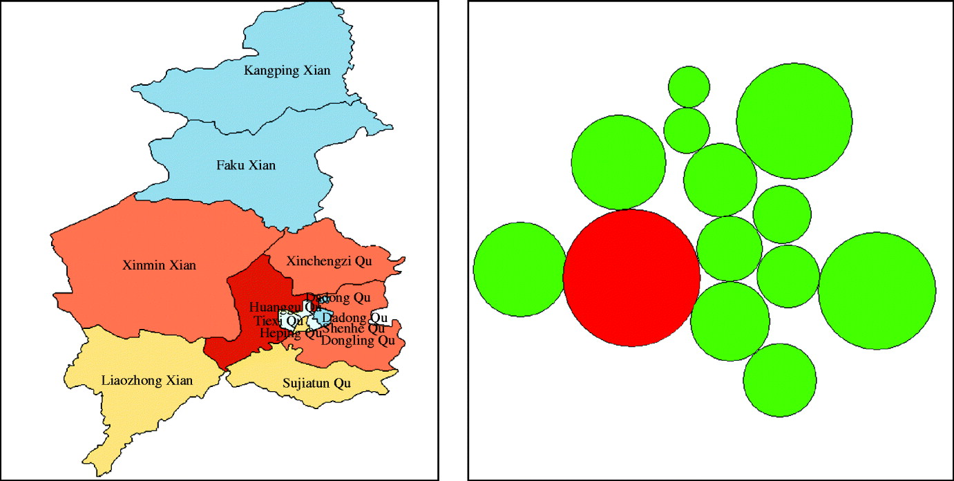
Fig. 2. Cartogram of haemorrhagic fever with renal syndrome in Shenyang, China, 1990–2003.
Among the 13 areas in Shenyang, five areas were low-endemic, five areas were medium-endemic, and three areas were high-endemic. The areas of the three types are displayed in a thematic map (Fig. 3).
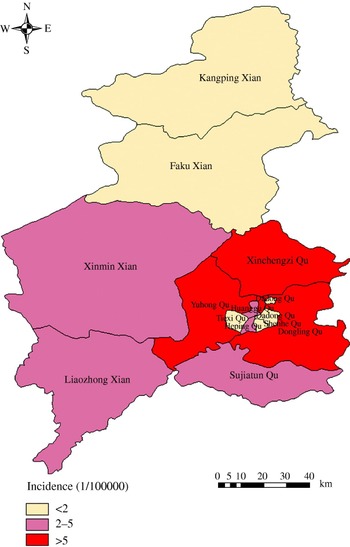
Fig. 3. Annualized average incidence of haemorrhagic fever with renal syndrome in Shenyang, China, 1990–2003.
The excess hazard map shows distribution of excess risk which was defined as a ratio of the observed number over the expected number of cases. Areas in blue had a lower risk than expected as indicated by excess risk of values of <1. In contrast, counties coloured red had a higher risk than expected or excess risk values >1 (Fig. 4). The excess risk is a non-spatial analysis which ignores the influence of spatial autocorrelation.

Fig. 4. Excess risk map of haemorrhagic fever with renal syndrome in Shenyang, China, 1990–2003.
A spatially smoothed percentile map for annual average incidence was created by correcting the variance in the variability of incidence, and six neighbours identified for each county by k-nearest-neighbour criterion provided the most appropriate map of smoothed incidence (Fig. 5).

Fig. 5. Spatial smoothed percentile map of haemorrhagic fever with renal syndrome in Shenyang, China, 1990–2003.
Spatial autocorrelation of HFRS in Shenyang
A Moran scatter plot was created and a significance assessment through a permutation test was implemented by global spatial autocorrelation analysis for annualized average incidence of HFRS (Fig. 6). The value listed at the top of the graph (−0·2413) was Moran's I statistic (Fig. 6 a). The scatter plot figure was centred on the mean with the axes drawn such that the four quadrants were clearly shown. Each quadrant corresponded to a different type of spatial autocorrelation: high-high and low-low for positive spatial autocorrelation; low-high and high-low for negative spatial autocorrelation. The two red dashed lines contained 95% of the distribution of Moran's I statistics computed in spatially random datasets. These slopes corresponded to the 2·5 and 97·5 percentiles of the reference distribution. As shown in the figure the actual Moran scatter-plot slope was well outside the range corresponding to the randomly permuted data. A histogram was generated by performing the significance assessment of Moran's I (Fig. 6 b). In addition to the reference distribution (in brown) and the statistic (yellow line), this graph listed the number of permutations and the pseudo-significance level in the upper left corner as well as the value of the statistic (−0·2413), and its theoretical mean (E[I]=−0·0833); the mean and standard deviation of the empirical distribution were −0·0848 and 0·0769, respectively. The statistic turned out to be significant for Moran's I at significance level of 0·05. These results implied that distribution of HFRS was spatially autocorrelated in Shenyang, i.e. HFRS cases in 13 areas in Shenyang, were not distributed randomly in space.
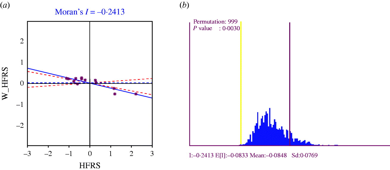
Fig. 6. (a) Moran scatter plot for annualized average incidence of haemorrhagic fever with renal syndrome (HFRS). (b) Histogram for significance assessment of Moran's I.
Spatial clustering of HFRS in Shenyang
Spatial cluster analysis of HFRS cases in 13 areas in Shenyang showed HFRS was not distributed randomly in space. Using the maximum spatial cluster size of 50% of the total population, one most likely cluster and two secondary clusters were identified (Fig. 7). The most likely cluster encompassed one area. The overall relative risk within the cluster was 3·673 (P=0·001) with an observed number of 530 cases compared to a calculated number of 165·51 expected cases. The two secondary clusters included one area, respectively, where the relative risk within a non-random distribution pattern was also significant (P=0·001) (Table 1).

Fig. 7. Spatial distribution of clusters of haemorrhagic fever with renal syndrome with significant higher incidence using the maximum spatial cluster size of 50% of the total population in Shenyang, China, 1990–2003.
Table 1. SaTScan statistics for the most likely spatial cluster, Shenyang, China, 1990–2003 (total population=6 699 631, total cases=3010)
* Number of observed cases in a cluster.
† Number of expected cases in a cluster.
Temporal clustering of HFRS in Shenyang
Temporal cluster analysis of HFRS cases in 1990–2003 in Shenyang showed HFRS was not distributed randomly in time. Using the maximum temporal cluster size of 50% of the total population, one most likely cluster was identified. The overall relative risk within the cluster was 3·673 (P=0·001) with an observed number of 2063 cases compared to a calculated number of 13 515·03 expected cases, and there was no secondary cluster (Table 2).
Table 2. SaTScan statistics for the most likely temporal cluster, Shenyang, China, 1990–2003 (total population=6 699 631, total cases=3010)
LLR, Log likelihood ratio; RR, relative risk.
* Number of observed cases in a cluster.
† Number of expected cases in a cluster.
Table 3. SaTScan statistics for the most likely space–time cluster, Shenyang, China, 1990–2003 (total population=6 699 631, total cases=3010)
LLR, Log likelihood ratio; RR, relative risk.
* Number of observed cases in a cluster.
† Number of expected cases in a cluster.
Space–time clustering of HFRS in Shenyang
Space–time cluster analysis of HFRS cases in 1990–2003 in 13 areas in Shenyang showed HFRS was not distributed randomly in space–time. Using the maximum spatial cluster size of 50% of the total population, and the maximum temporal cluster size of 50% of the total population, a most likely cluster and a secondary cluster were identified (Fig. 8). The most likely cluster encompassed six areas (three belonging to urban areas and three belonging to suburban areas) from 1998 to 2003. The overall relative risk within the cluster was 2·625 (P=0·001) with an observed number of 1212 cases compared to a calculated number of 615·01 expected cases. The secondary cluster encompassed four areas (three areas belonging to counties and one area belonging to suburban areas) from 1995 to 1996, where the relative risk within a non-random distribution pattern was also significant (P=0·001) (Table 3).

Fig. 8. Space–time distribution of clusters of haemorrhagic fever with renal syndrome with significant higher incidence using maximum spatial cluster size of 50% of the total population, and the maximum temporal cluster size of 50% of the total population in Shenyang, China, 1990–2003.
DISCUSSION
Cluster analysis is important in epidemiology to detect aggregation of disease cases, to test the occurrence of any statistically significant clusters, and ultimately to find evidences of risk factors. Cluster analysis identifies whether geographically or temporally grouped cases of disease can be explained by chance or are statistically significant.
Using GIS-based temporal, spatial and space–time scan statistics we investigated the temporal, spatial and space–time distribution of HFRS cases and identified areas and periods with high endemic HFRS and clustering patterns. This study showed that the geographic, temporal and space–time distribution patterns of HFRS cases in Shenyang was non-random.
Spatial cluster analysis identified one most likely cluster and two secondary clusters based on a maximum spatial cluster size of 50% of the total population which had a statistically significant (P<0·001) increased HFRS risk. There were three suburban areas included in total, and all the urban areas were surrounded by these three areas. Chinese cabbage was mainly planted in the Shenyang suburbs in summer and autumn [Reference Zhang27], rice was mainly planted in the southern and western part of Shenyang, and corn and sorghum were mainly planted in the northern part of Shenyang. Accordingly, we can conclude that HFRS cases are more likely to occur in those areas planting Chinese cabbage. One possible reason is that the life-cycle of mice may be related to the type of crop.
Temporal cluster analysis identified one most likely cluster based on a maximum temporal cluster size of 50% of the total population which had a statistically significant (P<0·001) increased HFRS risk, and the time-frame was 1998–2003. Some scholars have reported risk factors for HFRS, e.g. climate, mice and occupation [Reference Bi28, Reference Bi29]. These authors found that mean minimum temperature, mean air pressure, amount of precipitation, autumn crop production and autumn density of mice were correlated with the incidence of HFRS in Yingshang County from 1980 to 1996. According to the temporal cluster analysis we can conclude these factors may result in the cluster, although there were no reports of these risk factors for HFRS in Shenyang.
Space–time cluster analysis identified one most likely cluster and one secondary cluster based on a maximum spatial cluster size of 50% of the total population and a maximum temporal cluster size of 50% of the total population which had a statistically significant (P<0·001) increased HFRS risk. This provided some evidence that the HFRS epidemic foci had changed from county to urban and suburban areas in Shenyang. One probable reason was urbanization, i.e. an increasing number of people moved to urban and suburban areas from the counties, another reason may be related to the change of mice species.
The process of cluster analysis in this study is as an ecological study. The objective was to determine if there was an association between certain areas and periods of HFRS with excess incidence. However, as an ecological study there are some potential limitations. An important weakness of our study was the ecological design, which includes no time-to-event data at the individual level, and confers risk of ecological fallacy. Therefore these results can not be extrapolated to the individual level. Another weakness was the socioeconomic, environmental and other factors; these were not taken into account due to non-availability of appropriate records of these factors. However, the cluster analysis does provide valuable information about geographic disparity of HFRS for further study in Shenyang.
GIS and GIS-based spatial, temporal, and space–time scan analysis may provide an opportunity to classify the epidemic situation of HFRS in Shenyang from 1990 to 2003. Spatial cluster analysis found three suburban areas where Chinese cabbage was mainly planted at increased risk of HFRS. We concluded that the life-cycle of mice in these areas may be different from those areas planting other crops. Temporal cluster analysis found one period increased the risk of HFRS. The difference of climate, mice and occupation, etc., may result in the cluster. Space–time cluster analysis found one most likely cluster and one secondary cluster. This result implied the HFRS epidemic foci had changed from county to urban and suburban areas, which may be related to urbanization. Another possible reason may be the change of mice species because of the ‘greenhouse’ effect. The present study only analyses the statistically significant clusters of HFRS in Shenyang, China. However, clusters identified with significantly high incidence of HFRS will be useful for investigating the underlying causes of increased risk. Future research could focus on the effect of various socioeconomic and environmental factors on the high occurrence of HFRS according to the different clusters. We believe that these analyses were helpful in meeting our objectives and should be used to supplement infectious disease investigation methods whenever they are applicable.
ACKNOWLEDGEMENTS
The study was supported by Natural Science Foundation of China (grant no. 30771860).
DECLARATION OF INTEREST
None.


