


INTRODUCTION
Despite the regularity with which seasonal influenza epidemics occur in temperate climates, the timing, duration and impact of these epidemics vary substantially from year to year. This presents an annual challenge for healthcare providers to deliver timely and proportionate responses. Being able to predict key attributes of an incipient seasonal influenza epidemic therefore represents an extremely valuable decision-support capability.
Previous studies have shown that Bayesian estimation techniques (‘filters’) can yield accurate predictions of epidemic peak timing many weeks in advance for US cities, by linking mechanistic infection models with Google Flu Trends (GFT) data [Reference Shaman and Karspeck1], and by combining GFT data with viral isolation data [Reference Yang, Karspeck and Shaman2].
We have previously tailored these methods for metropolitan Melbourne (Australia) and GFT data, showing that forecasts with similar accuracy can be obtained [Reference Moss3]. However, the relationship between GFT data and actual influenza incidence is tenuous in the United States [Reference Lazer4] and there is no reason to expect the contrary in Australia. Ideally, epidemic forecasts should instead be generated from data that is as closely related to actual incidence as possible. There are several sources of influenza and influenza-like illness (ILI) surveillance data for metropolitan Melbourne, and our group has previously evaluated the statistical biases in these systems [Reference Thomas5].
In this study we applied a Bayesian forecasting method (the bootstrap particle filter) to each of the surveillance systems in turn and compared the resulting forecast skill. We then fused data from all three systems simultaneously to evaluate whether forecasting skill was improved by accounting for all of available data, compared to fusing data from any single system.
METHODS
Surveillance systems
The surveillance systems considered in this study were:
-
• Victorian Department of Health & Human Services (VDHHS) laboratory-confirmed influenza notifications [Reference Clothier6].
-
• Victorian Sentinel Practice Influenza Network (VicSPIN, previously known as General Practitioner Sentinel Surveillance, GPSS) reports of ILI prevalence in patients at participating sites [Reference Clothier6, Reference Kelly7].
-
• National Home Doctor Service (NHDS, previously known as Melbourne Medical Deputising Service, MMDS) reports of ILI prevalence in home visits, which are provided on weekends, public holidays, and after-hours on weekdays [Reference Clothier6].
Data for the 2010–2014 influenza seasons were used (see Figs 1 and 2). We removed two outliers in the NHDS data (November 2013 and January 2014) and one outlier in the VicSPIN data (October 2011, 174 patients, 2·9% with ILI symptoms). Although the total number of patients seen each week by GP clinics recruited in the VicSPIN schemes varies from week to week (μ = 6900, σ = 1000) there is a clear linear relationship between the number of patients with ILI and the percentage of patients with ILI (R 2 = 0·9863). This suggests that these two measures of influenza activity are almost equivalent and should yield near-identical forecasts.
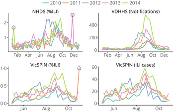
Fig. 1. The data obtained from each surveillance system for metropolitan Melbourne. Outliers (hollow circles) were removed prior to forecasting. NHDS, National Home Doctor Service; VDHHS, Victorian Department of Health & Human Services; VicSPIN, Victorian Sentinel Practice Influenza Network.
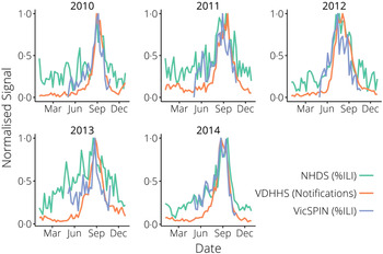
Fig. 2. The surveillance data, normalized yearly for comparison between systems. NHDS, National Home Doctor Service; VDHHS, Victorian Department of Health & Human Services; VicSPIN, Victorian Sentinel Practice Influenza Network.
A previous analysis of these same systems for 2009–2012 [Reference Thomas5] made the following observations for the 2010–2012 seasonal influenza outbreaks:
The data obtained from each of these systems exhibit over-dispersion (relative to the Poisson distribution) to different degrees and were subsequently modelled as independent negative binomials. The NHDS and VicSPIN data were found to have greater over-dispersion than the VDHHS data, presumably due (at least in part) to the presence of other ILIs (e.g. rhinoviruses).
Baseline activity and epidemic duration varied across seasonal influenza outbreaks (2010–2012); the only significant effect of surveillance system was a slightly lower baseline activity for the NHDS. Surveillance systems did, however, exhibit a significant effect on final size, with much smaller final sizes for VicSPIN and NHDS.
Peak timing was also sensitive to surveillance system: the VicSPIN and NHDS peaks occurred 2 weeks and 1 week earlier than the VDHHS peak, respectively (2010–2012). This cannot be explained by testing or reporting delays, since it was observed when using the date of presentation for all three systems. Both syndromic surveillance systems reported two local maxima in the 2014 season, occurring 3–4 weeks apart; the first coinciding with the VDHHS peak in late August. The second local maxima was smaller than the first for the VicSPIN data, but was larger than the first for the NHDS data, meaning that the VicSPIN and VDHHS peaks coincided and the NHDS peak occurred 4 weeks later.
Influenza transmission model
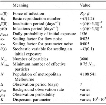
We used an SEIR compartment model with homogeneous mixing to represent the infection process [equations (1)–(4), parameters listed in Table 1]. This model admits stochastic noise in flows between compartments [equations (5)–(8)] and in model parameters [equation (9)]. An epidemic starts with a single stochastic exposure event [equation (10)] that occurs with daily probability p seed and is introduced into a completely susceptible population.
 $$\displaystyle{{{\rm d}S} \over {{\rm d}t}} = - \alpha SI - \zeta _S - \theta _{{\rm seed}}, $$
 $$\displaystyle{{{\rm d}E} \over {{\rm d}t}} = \alpha SI + \zeta _S + \theta _{{\rm seed}} - \beta E - \zeta _E, $$
 $$\displaystyle{{{\rm d}I} \over {{\rm d}t}} = \beta E + \zeta _E - \gamma I - \zeta _I, $$
 $$\displaystyle{{{\rm d}R} \over {{\rm d}t}} = \gamma I + \zeta _I, $$
 $$\zeta _{(S,E,I)}\, {\rm \sim {\cal N}}(\mu = 0,\sigma = \sigma _{(S,E,I)} ),$$
 $$\sigma _S = \kappa _F \cdot \sqrt {\alpha SI}, $$
 $$\sigma _E = \kappa _F \cdot \sqrt {\beta E}, $$
 $$\sigma _I = \kappa _F \cdot \sqrt {\gamma I}, $$
 $$\displaystyle{{{\rm d}\alpha} \over {{\rm d}t}},\displaystyle{{{\rm d}\beta} \over {{\rm d}t}},\displaystyle{{{\rm d}\gamma} \over {{\rm d}t}}\,{\rm \sim {\cal N}}(\mu = 0,\sigma = \kappa _P ),$$
 $$\theta _{\rm seed} = \left\{\matrix{\displaystyle{1 \over N} & {\rm if}\;S(t) = 1\;{\rm and}\;\theta (t) \lt p_{\rm seed} \cr 0 & {\rm otherwise}.\hfill} \right.$$
Table 1. Parameter values for (i) the transmission model; (ii) the bootstrap particle filter; and (iii) the observation model
Model estimation
We used the bootstrap particle filter to identify which realizations of the transmission model were the most likely to yield in silico observations consistent with the weekly surveillance data. For each of the three surveillance systems, and for each of the 2010–2014 calendar years, a finite set of model vectors (‘particles’) were used to approximate the continuous model-space likelihood distribution. Each particle contains both the state variables and model parameters of the transmission model [equation (11); parameter values are drawn from the prior distributions listed in Table 1]. Initially, all particles have identical weights [equation (12)], which are subsequently adjusted in proportion to the likelihood of giving rise to each observation [equations (13)–(14)]. When too much of the probability mass accumulates in a small subset of the particles, the mass is redistributed by resampling the particles in proportion to their weights. This is performed using the systematic method, as described by Kitagawa [Reference Kitagawa8], when the effective number of particles [equation (15)] falls below the threshold N min (defined in Table 1).
 $${\bf x}_{\bf t} = [S(t),E(t),I(t),R(t),\alpha (t),\beta (t),\gamma (t)]^T, $$
 $$w_i (0) = \left( {N_{{\rm px}}} \right)^{ - 1}, $$
 $$w^{\prime}_i (t \vert {\bf y}_{\bf t} ) = w_i (t - 1) \cdot P({\bf y}_{\bf t} \vert {\bf x}_{\bf t}^{\bf i} ;k),$$
 $$w_i (t \vert {\bf y}_{\bf t} ) = w^{\prime}_i (t) \cdot \left( {\sum\limits_{j = 1}^{N_{{\rm px}}} w^{\prime}_j (t)} \right)^{ - 1}, $$
 $$N_{{\rm eff}} (t) = \left( {\sum\limits_{\,j = 1}^{N_{{\rm px}}} \left[ {w^{\prime}_j (t)} \right]^2} \right)^{ - 1}. $$
Observation models
For each of the three surveillance systems, we characterized the annual signal as comprising a background rate of presentation p bg, and an observation probability p id that represents the probability of an infection being symptomatic and observed, and acts as a scaling factor between model incidence and the surveillance data. We assume that these parameters remain constant for the duration of each influenza season. Note that interpretation of the background rate is system-dependent. For laboratory-confirmed cases, it represents the low level of endemic activity observed outside of the influenza season (presumably due to importation events and limited subsequent transmission). These cases are treated as observation noise and are not represented as infections in the transmission model. For ILI surveillance systems, it also includes any other pathogen that results in influenza-like symptoms.
The probability that an individual becomes infectious (p
inf) during the interval $(t - \Delta, t]$
is defined as the fraction of the population that became infectious over that interval [equation (16)]. The probability of a case being observed by a given system is therefore the sum of the probabilities of two mutually exclusive events [equation (17)]: becoming infectious and then being identified, or contributing to the background signal. We modelled each surveillance system as a (conditionally independent) negative binomial in order to define the likelihood of an observation
$(t - \Delta, t]$
is defined as the fraction of the population that became infectious over that interval [equation (16)]. The probability of a case being observed by a given system is therefore the sum of the probabilities of two mutually exclusive events [equation (17)]: becoming infectious and then being identified, or contributing to the background signal. We modelled each surveillance system as a (conditionally independent) negative binomial in order to define the likelihood of an observation ${\bf y}_{\bf t} $
for a given particle
${\bf y}_{\bf t} $
for a given particle ${\bf x}_{\bf t} $
. The dispersion parameter k controls the mean-variance relationship for each surveillance system [equations (18)–(19)].
${\bf x}_{\bf t} $
. The dispersion parameter k controls the mean-variance relationship for each surveillance system [equations (18)–(19)].
 $$p_{{\rm inf}} (t,\Delta ) = S(t - \Delta ) + E(t - \Delta ) - S(t) - E(t),$$
 $$p_{{\rm ili}} (t,\Delta ) = p_{{\rm inf}} (t,\Delta ) \cdot p_{{\rm id}} + [1 - p_{{\rm inf}} (t,\Delta )] \cdot \Delta \cdot p_{{\rm bg}}, $$
 $$P({\bf y}_{\bf t} \vert {\bf x}_{\bf t} ;k) = \displaystyle{{\Gamma ({\bf y}_{\bf t} + k)} \over {\Gamma (k) \cdot {\bf y}_{\bf t} !}} \cdot (\,p_{\rm k} )^k \cdot (1 - p_{\rm k} )^{{\bf y}_{\bf t}}, $$
 $$p_{\rm k} = \displaystyle{k \over {k + N \cdot p_{{\rm ili}}}}. $$
For the NHDS and VicSPIN data we fixed the background observation rate p bg over the 2010–2014 calendar years, since the out-of-season ILI levels remained relatively stable over this period. However this was not the case for the VDHHS notifications data, which exhibited substantial annual changes in out-of-season notification counts. Accordingly, we estimated the mean out-of-season notification rate separately for each year (by calculating the mean over the first few calendar months) and defined background observation rates relative to this annually varying quantity (see Table 2). Note that the out-of-season notification rate increased substantially over this 5-year period (a mean annual increase of 6·2 notifications per week, R 2 = 0·78). This is consistent with observations that increased testing has caused notification counts to substantially increase in recent years, independently of disease burden [Reference Lambert9–Reference Fielding12].
Table 2. Estimated mean out-of-season VDHHS influenza notification rates for each influenza season, and the associated background observation rates used for the observation models (‘−5’, ‘+0’, ‘+5’; defined relative to the mean estimates)
VDHHS, Victorian Department of Health & Human Services.
For all three surveillance systems, we assessed forecasting performance over a wide range of observation probabilities (p id).
Epidemic forecasts
Given a sequence of observations {y
1, …, y
k
} and prior distribution for the initial particle ${\bf x}_{\bf 0} $
, the bootstrap particle filter (or any other Bayes filter) can be used to estimate the posterior distribution for
${\bf x}_{\bf 0} $
, the bootstrap particle filter (or any other Bayes filter) can be used to estimate the posterior distribution for ${\bf x}_{\bf k} $
. By taking a finite number of samples from the posterior and simulating forward in time, an ensemble of trajectories is obtained. With a particle filter, the existing particles serve as the posterior samples and their weights
${\bf x}_{\bf k} $
. By taking a finite number of samples from the posterior and simulating forward in time, an ensemble of trajectories is obtained. With a particle filter, the existing particles serve as the posterior samples and their weights $w_i (t)$
represent the likelihood of each trajectory. A probabilistic forecast is obtained by estimating the expected values of future observations
$w_i (t)$
represent the likelihood of each trajectory. A probabilistic forecast is obtained by estimating the expected values of future observations $\bar y(t)$
[equation (20)]. Here, we report the median, 50% and 90% credible intervals for
$\bar y(t)$
[equation (20)]. Here, we report the median, 50% and 90% credible intervals for $\bar y(t)$
.
$\bar y(t)$
.
 $$\bar y(t) = \{ N \cdot p_{{\rm ili}} (t,\Delta )\} \;\forall \;{\bf x}_{\bf t}^{{\bf (i)}}. $$
Because each forecast comprised estimates of weekly incidence for every 7-day period from the forecasting date until the end of the year, peak forecast incidence could occur on any weekday, even though all of the surveillance data are reported weekly. Accordingly, we defined forecast accuracy as the weighted fraction of all trajectories whose peak occurred within 10 days of the observed peak, equivalent to rounding to the nearest reporting day (i.e. ±3 days) and then applying a threshold of ±1 week.
Similar to our previous forecasting study, we took the mean of these fractions over the 8 weeks prior to the observed peak – similar in concept to calculating the area under a ROC curve – to ‘score’ observation models for a given influenza season, and subsequently ranked observation models by their mean scores over the 2010–2014 seasons. The simulation and ranking scripts, and instructions for their use, are included in the Supplementary material.
RESULTS
Annual forecasting performance
The best forecasting performances obtained from each surveillance system over the 2010–2014 influenza seasons are shown in Figure 3 and allow us to make several observations about the variation between seasons. The 2010 season was particularly mild and short, making it difficult to distinguish from the background signal. This is demonstrated by the low forecasting scores for 2010 across all three systems and for all observation probabilities; the best forecasts were obtained at the minimum observation probabilities, indicating that this was the only way to relate the transmission model to such a small epidemic. In contrast, high forecasting scores were obtained for 2011 and 2012 across all three surveillance systems (k ⩾ 10, best results for k = 100). Good forecasts were also obtained from the VDHHS data for 2013 and 2014, but the syndromic systems yielded poorer performances for these seasons; the VicSPIN forecasting scores were moderate for 2013 and low for 2014, while the NHDS forecasting scores were low for both seasons.
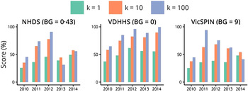
Fig. 3. Annual forecasting performance for the three surveillance systems (shown for each value of the dispersion parameter k and with a single background rate for each system), illustrating for which seasons reliable forecasts could be obtained in the 8 weeks prior to the peak when using the optimal observation probability. NHDS, National Home Doctor Service; VDHHS, Victorian Department of Health & Human Services; VicSPIN, Victorian Sentinel Practice Influenza Network.
Retrospective peak timing forecasts for each the 2010–2014 influenza seasons, using the single best observation model for each surveillance system, are shown in Figure 4. The forecasts for 2010 again demonstrate that the 2010 season was particularly difficult to forecast, since it was a particularly mild and brief season. The variance of the 2010 NHDS forecast oscillated over time and, while it remained stable and accurate in the final 2 weeks prior to the peak, the variance was sufficiently large to suggest little, if any, confidence in the prediction. The 2010 VDHHS forecast was narrow and stable in the final 4 weeks prior to the peak, but the prediction was inaccurate (5 weeks later than the actual peak). The 2010 VicSPIN forecast only became narrow in the week prior to the actual peak, and was also inaccurate (3 weeks late). For each of the remaining seasons (2011–2014), accurate predictions of the peak timing were obtained well in advance from the influenza case notifications. The GP sentinel surveillance data (VicSPIN) yielded accurate forecasts for the 2011, 2012 and 2013 seasons, but the timing of the 2014 peak was much later than predicted. The home doctor surveillance data (NHDS) yielded accurate forecasts for the 2011 and 2012 seasons, but the timing of the 2013 and 2014 peaks were much later than predicted.
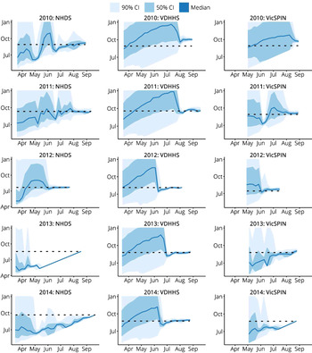
Fig. 4. Retrospective forecasts for the 2010–2014 influenza seasons in Melbourne, as produced by the single best observation model for each system (i.e. the same observation model was used for every season). These plots show the confidence intervals of the peak timing predictions (y-axis) plotted against the forecasting date (x-axis) for the period prior to the actual peak. Peak timing was accurately predicted in general; exceptions were 2013 and 2014 for the NHDS data, 2010 for the VDHHS data, and 2010 and 2014 for the VicSPIN data. NHDS, National Home Doctor Service; VDHHS, Victorian Department of Health & Human Services; VicSPIN, Victorian Sentinel Practice Influenza Network.
Further examination of the forecasts shown in Figure 4 also allows us to identify when we can expect to place confidence in the model predictions. When the credible intervals for the peak timing are broad, the predictions are clearly uncertain and may even reflect uncertainty in the mere presence of an epidemic. When the credible intervals for the peak timing become very narrow, several different outcomes can be observed:
-
• The credible intervals subsequently widen, indicating a loss of confidence (e.g. NHDS 2010); the credible intervals may narrow again at a later time (e.g. VicSPIN 2011).
-
• The predicted timing is both stable and accurate (e.g. VDHHS 2011–2014).
-
• The predicted timing is stable but is inaccurate (e.g. VDHHS 2010); this may indicate particle degeneracy (i.e. when the particles have failed to thoroughly explore the model space).
-
• The predicted timing does not remain stable, even though the credible intervals remain narrow (e.g. NHDS 2013, VicSPIN 2014); this typically indicates the lack of a clear epidemic signal or particle degeneracy.
With the exception of the very mild 2010 season, it is clear that confidence should be placed in the epidemic forecasts when the credible intervals are narrow (i.e. when the forecast variance is low) and the predictions remain stable in response to subsequent observations.
Net forecasting performance
The mean forecasting performance for each observation model over the 2010–2014 seasons is shown in Figure 5. Each curve represents a series of observation models that have the same background observation rate and dispersion parameter, and differ only in their observation probabilities. These curves all exhibit a bell shape, indicating that optimal forecasts (those with the best mean performance over these seasons) are obtained only within a small range of observation probabilities. It is therefore paramount to be able to estimate the appropriate observation probability during (or prior to) the nascent stage of an epidemic, in order to maximize the likelihood of producing reliable forecasts. As the dispersion parameter is increased (i.e. as we assume that there is less variance in the observed data) the curves retain a bell shape and the forecasting performance is increased. However the curves also become less smooth and exhibit sensitivity to small changes in the observation probability. This indicates we are approaching the point where there is greater variability in the observed data than in the observation model (i.e. that the observation model is becoming under-dispersed) and too much information is being inferred from each datum. This suggests an approximate upper bound on k.
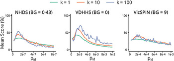
Fig. 5. The mean forecasting performance over the 2010–2014 influenza seasons for each surveillance system as a function of the observation probability p id, shown for each value of the dispersion parameter k and with a single background rate for each system. NHDS, National Home Doctor Service; VDHHS, Victorian Department of Health & Human Services; VicSPIN, Victorian Sentinel Practice Influenza Network.
The single best observation model – the one with the highest mean score in Figure 5 – used the VDHHS data and the estimated out-of-season notification rates (‘+0’, refer to Table 2), with k = 100 and an observation probability of p id = 0·00225 (~1 in 450 ‘actual’ cases). Since such fine-tuning is not practical when forecasting a live epidemic, it is critical to identify how to obtain robust, near-optimal forecasts. It is clear from Figure 5 that the forecasts obtained from the VDHHS notifications data consistently out-performed the NHDS and VicSPIN forecasts, suggesting that the VDHHS data might more precisely characterize each seasonal influenza outbreak than the other (syndromic) surveillance systems. Near-optimal forecasts were obtained from the VDHHS data over a reasonably broad range of observation probabilities (0·00125 ⩽ p id ⩽ 0·003).
Retrospective forecasting of the 2009 H1N1 pandemic
Having identified the observation models that produced the best forecasts for the 2010–2014 seasonal influenza epidemics, we then used these observation models to produce retrospective forecasts for the 2009 H1N1 pandemic in Melbourne, as characterized by the same surveillance systems. Initially, laboratory testing of all suspected influenza patients was authorized [Reference Fielding13]. From June, however, testing was only recommended only for those with moderate or severe disease and those in particular risk groups [Reference Fielding13]. Accordingly, the influenza notifications data for 2009 has a huge peak at the end of May (1025 confirmed cases) as a result of the elevated ascertainment, and a second, smaller peak on June 21 (533 confirmed cases) that we assume is the ‘true’ peak in this data. To provide appropriate observations to the particle filter, it was necessary to scale the case counts for the weeks ending 24 May, 31 May, and 7 June. For simplicity we scaled these counts by 1/4 on the grounds that the resulting epidemic curve looked reasonable (we did not fit this scaling factor or explore other values). Note that it is not clear how to make such a ‘correction’ during an actual outbreak, particularly in the absence of denominator data, as is the case for influenza testing in Australia. As shown in Figure 6, we were able to obtain accurate predictions of the peak timing from each surveillance system 3–4 weeks in advance of the observed peak.
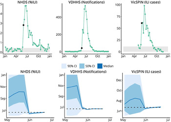
Fig. 6. Retrospective forecasts for the 2009 H1N1 pandemic in Melbourne. The top row shows the surveillance data from each system (VDHHS notification counts modified as described in the text); black points indicate the time at which the variance in peak timing predictions rapidly decreased, the grey regions indicate values less than the background rate. The bottom row shows the confidence intervals of the peak timing predictions (y-axis) plotted against the forecasting date (x-axis) for the period prior to the actual peak. Peak timing was accurately predicted 3 weeks prior to the actual peak (NHDS and VicSPIN data) and 4 weeks prior to the actual peak (VDHHS data). NHDS, National Home Doctor Service; VDHHS, Victorian Department of Health & Human Services; VicSPIN, Victorian Sentinel Practice Influenza Network.
This indicates that it is not unreasonable to calibrate observation models against seasonal influenza outbreaks in order to generate forecasts during future pandemic events. Of course, a truly novel or especially virulent strain may confound these observation models, due to changes in, e.g. population susceptibility, health-seeking behaviours, and testing and surveillance recommendations. Spurious or suspect observations may also be ignored or adjusted once it becomes apparent that they are questionable (presumably within a few weeks of being reported) to improve forecast robustness.
Forecasting with multiple data sources
Having identified the observation models that produced the best forecasts for the 2010–2014 influenza seasons, we also evaluated the forecasting performance for each of these seasons when we used all three data sources simultaneously; this required a definition of the ‘true peak’ for each season. In 2009 all three surveillance systems reported the same peak timing, but this did not occur in any of the 2010–14 seasons. Since the VDHHS influenza notifications data is the most direct observation of influenza activity, we used this data to define the ‘true peak’. The likelihood of the set of simultaneous observations $\{ {\bf y}_{\bf t}^{\bf i}, \ldots, {\bf y}_{\bf t}^{\bf n} \} $
for a given particle was defined by equation (21); we assumed that, given the true incidence, all of the observation processes are independent.
$\{ {\bf y}_{\bf t}^{\bf i}, \ldots, {\bf y}_{\bf t}^{\bf n} \} $
for a given particle was defined by equation (21); we assumed that, given the true incidence, all of the observation processes are independent.
 $$P(\{ {\bf y}_{\bf t}^{\bf 1}, \ldots, {\bf y}_{\bf t}^{\bf n} \} \vert {\bf x}_{\bf t} ;k) = \prod\limits_{i = i}^n P({\bf y}_{\bf t}^{\bf i} \vert {\bf x}_{\bf t} ;k).$$
The out-of-season and peak notification levels vary from year to year (Fig. 1). It is understood that the influenza burden varied over the 2010–2014 seasons (e.g. 2010 was particularly mild) and therefore a variation in peak magnitude is to be expected. However the syndromic surveillance systems reported substantially less year-to-year variation in burden than was observed in the VDHHS data, and FluCAN hospital admissions data (not shown here) also suggest that the peak notification levels are not representative of the relative burden of each season [Reference Cheng14–Reference Cheng18]. The consistency of the syndromic surveillance data might therefore be expected to provide additional insight into each influenza season (particularly in the early stages) and therefore improve the forecasting performance, when compared against forecasts generated solely from the VDHHS notifications data.
The resulting forecasts demonstrate that simply using observations from all three surveillance systems does not necessarily improve the forecasting performance and, indeed, can even reduce performance. Differences were only observed in two of the five influenza seasons. In 2011, using all three data sources substantially improved the forecast accuracy in the 5 weeks prior to the peak, and also reduced the forecast variance. In 2013, the use of all three data sources reduced the forecast accuracy 2–5 weeks prior to the peak and increased the forecast variance over this same period.
The peak timing predictions for both sets of forecasts in these two seasons are shown in Figure 7. The intervals where they differ substantially in accuracy and variance are illustrated by the vertical dashed lines. These plots demonstrate that the inclusion of the two syndromic data sources have a minimal effect on the forecast predictions.
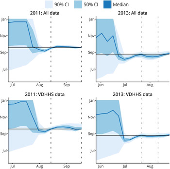
Fig. 7. A comparison of peak timing predictions when using data from all three surveillance systems (‘All data’) and when only using Victorian Department of Health & Human Services (VDHHS) notifications data (‘VDHHS data’). The intervals where these two sets of forecasts differed in accuracy and variance are indicated by the vertical dashed lines. Using all available data is seen to have a minimal effect on the peak timing predictions.
The most salient point to draw from these observations is that the use of multiple data sources does not necessarily provide any benefit over using a single data source of good quality. This suggests that complementary data streams may need to capture very different aspects of disease activity and may only provide useful information at specific stages of an epidemic. For example, FluCAN reports hospitalizations with confirmed influenza at several sentinel hospitals in Victoria [Reference Cheng14–Reference Cheng18], but weekly cases are sufficiently few that this may only provide additional information if additional hospitals can be recruited.
DISCUSSION
Principal findings
VDHHS laboratory-confirmed influenza notification counts consistently yielded more accurate and earlier forecasts of peak timing than did the data from either of the syndromic surveillance systems. For all three systems, observation models were identified that yielded good forecasts across all five of the influenza seasons under consideration (2010–2014, median effective reproduction number R eff = 1·1−1·35). These same observation models also yielded accurate predictions of the peak timing for the 2009 H1N1 outbreak in Melbourne, 3–4 weeks in advance of the observed peak (although the notification counts had to be adjusted to account for drastic changes in testing levels). Simultaneously fusing data from all surveillance systems did not appreciably improve forecasting performance.
These results suggest that (a) confirmed influenza cases are a more reliable data source for influenza forecasting than are syndromic data sources; (b) syndromic surveillance data are nevertheless capable of yielding good forecasts; (c) in the event of a pandemic, where testing levels may vary substantially (e.g. influenced by actual and perceived threat [Reference Kaczmarek11]), syndromic surveillance data may be a more stable data source for forecasting purposes. We further hypothesize that synthesis of data from multiple sources may only improve forecast performance if these sources characterize complementary aspects of disease activity (e.g. hospitalizations, healthcare-seeking behaviour).
These findings are consistent with those reported by Thomas et al. [Reference Thomas5], who observed that the choice of surveillance system significantly affected the inferred epidemic curve, peak timing, final epidemic size, and baseline influenza activity, even after adjusting for age, geographical region, and year. They also observed that the syndromic data were significantly more over-dispersed than the notifications data (indicating greater variability in syndromic case counts) which is consistent with the relative forecasting performances of the three systems as reported here. Furthermore, their findings were consistent with previous observations in Victoria and throughout Australia that testing rates have increased since 2009, while ILI rates have not increased proportionately [Reference Kelly10].
Study strengths and weaknesses
A key strength of this study is that we have evaluated the forecasting performance obtained from each surveillance system over each of the available influenza seasons, and can contrast and compare their predictive powers. This is a clear demonstration of how the data collection characteristics of any real-world surveillance system can be evaluated on its ability to yield precise and accurate forecasts, and could conceivably inform future surveillance investment efforts to further develop this predictive capacity.
Perhaps the greatest weakness of this study is that we only have five influenza seasons (i.e. five samples per surveillance system) against which to evaluate the forecasts. Since no two influenza seasons are exactly alike (Fig. 1), it would be instructive to have a larger collection of seasonal influenza epidemics at our disposal. Since we expect that these surveillance systems may exhibit changes in ascertainment and other characteristics over time, it would be preferable to have similar data for the same influenza seasons in other Australian cities than to have data from the same surveillance systems for the past, say, 20 years.
Comparison with other studies
In contrast to other infectious disease forecasting studies, we have compared multiple sources of surveillance data for their ability to yield accurate predictions of epidemic peak timing well in advance, and have identified relative strengths and weaknesses of each system for this purpose. Other studies have used a single data source [Reference Shaman and Karspeck1, Reference Chan19, Reference Ong20] or a primary data source that was modulated by a secondary data source (‘ILI+’) [Reference Shaman21, Reference Yang22]; in both cases single datasets were used to generate and evaluate the forecasts.
The ‘ILI+’ metric, where weekly ILI rates are multiplied by the percentage of influenza-positive tests for that week, is intended to better represent influenza incidence [Reference Shaman21, Reference Yang22]. However, negative tests are not notifiable in Australia and are generally reported only by public laboratories, which represent a diminishing proportion of Victorian influenza notifications [Reference Lambert9]. Therefore, ‘ILI+’ may not be appropriately representative of influenza incidence in Victoria.
In a previous study, we generated retrospective forecasts for seasonal influenza outbreaks in metropolitan Melbourne using GFT data [Reference Moss3]. In both studies we have observed that choosing an appropriate value for the dispersion parameter (k) is a critical balancing act. If the dispersion is too high (i.e. k is too small), not enough information is inferred from the data. If the dispersion is too low (i.e. k is too large), too much confidence is placed in the data and particle degeneracy is frequently observed. With GFT data we obtained optimal forecasts with a moderate amount of dispersion (k = 10), while in this study we obtained optimal forecasts when assuming that the data are less dispersed (k = 100). This is evidence that each of the surveillance systems considered in this study provide better characterisations of seasonal influenza activity than does the GFT data.
We have shown that using laboratory-confirmed influenza cases yielded more reliable forecasts than were obtained using syndromic data. This conclusion may appear both obvious and necessary, since RT–PCR tests are inherently more specific than are syndromic ILI diagnoses. However, this data source is also highly susceptible to changes in ascertainment (as shown by the change in out-of-season notification levels from year to year) and only captures the very tip of the true disease prevalence (the ‘burden of illness pyramid’ [Reference Wheeler23, Reference O'Brien24]), while the syndromic surveillance systems exhibited greater stability in both the out-of-season ILI levels and the magnitude of the seasonal peaks. One drawback of using laboratory-confirmed cases is the inherent delay, since specimens must be collected from patients, sent to laboratories, tested, and then reported to the VDHHS. However, in this retrospective setting, more precise forecasts were obtained, and further in advance, when using this data than when using syndromic surveillance data.
Accordingly, while we may have expected that the confirmed influenza cases would be the best data source for forecasting, it was certainly not a guaranteed outcome. And indeed, in the event of a pandemic where testing recommendations may differ greatly from seasonal influenza, it appears much easier to calibrate the observation models for the syndromic surveillance systems than for the confirmed influenza cases.
The true value of these forecasting methods lies in (i) accurately predicting the behaviour of future epidemics while they are in a nascent stage; and (ii) of equal importance, being able to identify when we should place great confidence in the predictions. Our results indicate that we should have confidence in the peak timing predictions when (and only when) the variance in these predictions is small and the predictions remain stable. These findings are consistent with other infectious disease forecasting studies [Reference Shaman and Karspeck1–Reference Moss3, Reference Shaman21, Reference Yang22, Reference Yang, Lipsitch and Shaman25, Reference Dawson, Gailis and Meehan26].
Meaning and implications
We have demonstrated that several existing surveillance systems that routinely operate in metropolitan Melbourne provide sufficient characterisation of seasonal influenza activity to permit accurate predictions of the epidemic peak many weeks in advance. In contrast to our previous study, which used GFT data, the insights and findings of this study are derived from direct, transparent measures of disease activity in the community. This allows us to place much greater confidence in the relevance and accuracy of the results. By also having separate measures of the predicted timing and the confidence in the predictions, these forecasting methods are particularly informative to healthcare providers, and may prove useful in guiding resource allocation (e.g. staffing levels) in future influenza epidemics.
Beyond the accuracy of the forecasts presented in this manuscript and the guidelines for gauging confidence in interpreting these forecasts, this study also demonstrates how to assess the predictive power of surveillance systems and, as such, can offer a measure of the relative ‘knowledge value’ of each system. An assessment framework of this kind can be used not only to compare different real-world systems, but also to evaluate a suite of hypothetical surveillance systems (via appropriate in silico experiments) in order to identify optimal data collection strategies and to inform future surveillance investment efforts.
Further work
Since each of these surveillance systems has unique characteristics and captures a different ‘view’ of the underlying influenza epidemic [27], it seems reasonable to expect that the forecasts could be substantially improved by synthesising the observations from each system into a single data stream for the particle filter, since this would allow the filter to incorporate a greater body of knowledge about each influenza season. The simplest manner in which this could be achieved is to re-weight the particles in response to all available observations at each time-step [i.e. assuming conditional independence as in equation (21)], using a single ‘best’ observation model for each surveillance system.
However, it is not clear how to sensibly evaluate forecasts obtained with such an approach since (i) the timing of the epidemic peak can differ substantially between systems (e.g. by 4 weeks in the 2014 season) and so there is no single ‘true peak’; and (ii) forecasts cannot be directly compared against the data from any one system, since the ‘best’ particles will be those that best agree with all three systems simultaneously. So while it is simple to run a Bayesian filter against the data from all three systems for any given influenza season, it is not at all apparent how one might sensibly evaluate the performance of these forecasts. In particular, it does not seem sensible to define the ‘true peak’ as the average of the peaks reported by each system, since the systems are observing fundamentally different aspects of each influenza epidemic. One possible solution is to evaluate forecasts against a single data source [Reference Santillana28], selected on the grounds that is understood to be, e.g. the most representative of the true epidemic. However, using the VDHHS notifications data as the best metric for forecast evaluation, we demonstrated that this approach does not guarantee any improvement in forecasting performance and may indeed achieve the opposite outcome. Techniques for estimating true incidence exist [Reference De29] and have been applied to, e.g. the 2009 H1N1 pandemic in the UK [Reference Baguelin30, Reference Presanis31] and the United States [Reference Presanis32], but are better suited to retrospective analyses than to providing a benchmark for forecast evaluation during an epidemic.
The extension of existing forecasting methods to combine data from disparate surveillance systems and define how to best evaluate the resulting forecast performance is a vital future development if these methods are to inform the preparation and delivery of proportionate healthcare responses in the future. It should also provide important insights into the ‘knowledge value’ of existing systems and help to guide future surveillance investment efforts.
SUPPLEMENTARY MATERIAL
For supplementary material accompanying this paper visit http://dx.doi.org/10.1017/S0950268816002053.
ACKNOWLEDGEMENTS
This work was funded by the DSTO project ‘Bioterrorism Preparedness Strategic Research Initiative 07/301’. James M. McCaw is supported by an ARC Future Fellowship (FT110100250). We thank Nicola Stephens, Lucinda Franklin and Trevor Lauer (VDHHS) and James Fielding, Heath Kelly and Kristina Grant (VIDRL) for providing access to, and interpretation of, Victorian influenza surveillance data. We also thank Branko Ristic (DST Group) for his advice and comments concerning particle filtering methods and observation models. We are grateful to the general practitioners who have generously chosen to participate in the VicSPIN sentinel surveillance system.
DECLARATION OF INTEREST
None.


