



INTRODUCTION
Tuberculosis (TB) is one of three high-burden endemic infections that are the focus of United Nations Development Programme (UNDP) targets [1]. The current burden is highest in low- and middle-income countries and is magnified in nations with generalized human immunodeficiency virus (HIV) epidemics [2]. Surveillance and monitoring of TB remains challenging. This is due, in part, to limitations in the tools available for quantifying key indicators.
The main epidemiological indicators that are relevant to TB control are incidence and prevalence of disease, case-fatality rate and prevalence of latent infection [Reference Dye3]. There are well-established methods for measuring the prevalence of disease and latent infection using cross-sectional surveys in representative samples of the population. Case-fatality rates can be quantified using routine surveillance data. However, estimation of incidence of disease is challenging [Reference Dye4]. Data on incidence are important because trends may provide the opportunity to evaluate the impact of TB control programmes and changes in risk factors for disease. Although disease notifications provide some information on incidence, this is almost always an under-estimate because of incomplete case detection. Unless the proportion of incident cases detected is known, disease incidence cannot be estimated from case notification data [Reference Dye5]. True incidence is also difficult to measure because of factors such as the difficulty in determining when symptoms commence, failure to differentiate TB from other diseases and failure of case notification [Reference Dye5].
To address the difficulties in estimating incidence, Styblo used a modelling approach to estimate key epidemiological ratios. He estimated that the ratio of the mortality to the incidence and prevalence of smear-positive TB was in the pattern 1:2:4. This is equivalent to saying that a smear-positive TB case remained infectious for 2 years, on average, with a 50% chance of dying from TB. His models applied to settings where treatment for TB was not routinely available. He further determined that the ratio of the percent annual risk of TB infection (ARTI) to the incidence of smear-positive pulmonary TB per 100 000 was 1:50 [Reference Styblo6]. These ratios were widely used around the world for some time [Reference Dye7].
Recent studies have shown that these ratios are not valid in several settings with functioning treatment programmes [Reference Dye7, Reference Van Leth8]. Furthermore, there is evidence that transmissibility varies widely between settings and, therefore, the ratio of disease incidence to ARTI is unlikely to be valid for all settings [Reference Dye7, Reference Van Leth8]. However, there has been little research attempting to devise new methods for estimating incidence. This leaves an important gap in the tools available for disease surveillance in settings where surveys have been performed.
The aims of this study were to re-examine the relationship between incidence and other indicators, determine the degree of deviation from Styblo's ratios in the presence of treatment and to develop a new method of estimating incidence from survey-derived indicators. Our approach uses an adaptation of a previously published TB model [Reference Blower9], which reflects TB epidemiology more realistically than the model used by Styblo.
METHODS
Model description
We adapted a model by Blower et al. [Reference Blower9], used originally to demonstrate the influence of epidemiological factors on the population dynamics of TB. Since our study is focused on the incidence and prevalence of infectious TB we excluded non-pulmonary TB as an outcome state and introduced a parameter describing treatment impact. The features that distinguish our model from Styblo's work [Reference Styblo6] are the specific parameterization of infection routes and demographic timescales, the inclusion of treatment and the potential for relapse following recovery from disease. Our study used no data and did not require ethical approval.
The model divides the population into several classes: individuals who are susceptible (S), latently infected individuals (E), individuals with infectious pulmonary TB (I) and recovered individuals (R). New susceptible individuals are born at fixed rate (Π) that ensures a stable population in the absence of disease. Natural mortality in individuals without active TB disease occurs at a constant rate (μ), which, in the base case, gives a mean life-expectancy of 70 years. We assume homogeneous mixing and uniform risks of infection with the force of infection (λ) expressed as the product of the density of infectious individuals and their per unit-time infectiousness (β). Figure 1 shows the model states and transitions (for the model equations, see Appendix).

Fig. 1. Model diagram showing classes and transitions of the model. Classes are susceptible (S), latently infected (E), infectious (I) and recovered (R). Transitions are births (Π), natural mortality (μ), primary infection (pβI/N), latent infection [(1 − p)βI/N], latent reactivation (v), mortality due to TB (μ T), relapse (ω) and recovery by treatment (τ) or natural (c) causes.
Infected individuals either progress rapidly to active disease (with probability P) or enter the latent class (with probability 1 − P), with progression to active disease determined by the reactivation rate (v). These rates are chosen so that in base case 5% of infections progress rapidly to disease and 5% progress to disease by reactivation from latent infection over a typical lifetime. Individuals with active TB suffer an additional risk of mortality (μ T). In the absence of treatment a proportion (c) of infectious individuals recover from TB, while recovered individuals can return to active disease through the relapse rate (ω) and are still latently infected with the disease post-recovery.
Treatment effects are captured by the addition of a single ‘treatment’ parameter (τ) to the model. There are a variety of methods for introducing treatment into models of TB and this is one of the simpler and more common approaches [Reference Ozcaglar10]. This parameter is the rate at which individuals with active TB move into the recovered class as a result of intervention. The effectiveness of the intervention can be considered to include the effectiveness of case-finding, case-holding, adherence to therapy and the efficacy of drug therapy. It represents the contribution of intervention programmes to the mean time until an individual with infectious TB is rendered non-infectious by treatment [or period of infectiousness (τ + c + μ + μ T)−1]. Treatment outweighs the other parameters in this period of infectiousness by an order of magnitude. All the consequences of therapeutic intervention are included through this parameter including impacts on mortality, transmission and rate of recovery.
Model parameters
Revised ratio
Over a long time period the distribution of the population in each state reaches a constant (or equilibrium) value. In this equilibrium situation, it is straightforward to show that the ratio of incidence to prevalence obeys the following equation:
 $$\displaystyle{{\rm{incidence}} \over {\,\rm{prevalence}}} = (\tau + c + \mu + \mu \rm{_T} ),$$
where the parameters τ, c, μ, μ T represent rates of treatment, natural recovery, mortality and TB-specific mortality respectively. The ratio is unaffected by the other model parameters, including transmissibility (β), reactivation or relapse rates. It should be noted that in our modelling approach ARTI and mortality are both directly proportional to prevalence and so ratios involving these quantities behave similarly to the ratio of incidence to prevalence. Details of the derivation of these ratios are given in the Appendix. The model was simulated using the ode45 solver in Matlab R2013b (www.mathworks.com/help/matlab/ref/ode45).
RESULTS
Figure 2 summarizes the model estimates for the main indicators, over time, in the absence of therapeutic intervention (‘treatment’). The model reveals an initial rapid rise in incidence and prevalence (Fig. 2a ) followed by a stable (endemic) phase. Due to the timescales of reactivation and relapse disease (Fig. 2b ), the epidemiology evolves slowly over a timescale from several decades to hundreds of years, depending on parameter values. The ratio of incidence to prevalence varies considerably during the epidemic period and then stabilizes rapidly once prevalence has peaked.

Fig. 2. (a) Modelled incidence and prevalence for a TB epidemic and then longer-term endemic equilibrium. (b) Modelled component of incidence over time. (c) Behaviour of the ratio of incidence to prevalence over time. Parameters for this simulation were β = 9, p = 0·075, v = 0·003915, μ = 0·0143, μ T = 0·4137, c = 0·072, ω = 0·007, Π = 2,860, τ = 0, S 0 = 200 000 and I 0 = 1.
Figure 3 shows the effect of introducing treatment into the model after it has reached the equilibrium state. The model predicts that the prevalence of TB disease will decline rapidly as soon as treatment is introduced, while the effect on incidence of TB disease is relatively smaller and more gradual. This is because, at equilibrium, most incident cases arise from reactivation of latent TB infection and to a lesser extent relapse of recovered cases. Incidence from these causes is unaffected by changes in infection prevalence. The decline in incidence of reactivation TB occurs at a significant delay, while incidence of relapse in people who have recovered after treatment for TB increases initially because the pool of recovered individuals increases in size when treatment is introduced. We note that while neither prevalence nor incidence reach equilibrium over the 40-year time-frame shown in Figure 3, the ratio of prevalence to incidence equilibrates very quickly. We also note that the introduction of treatment substantially changes the incidence to prevalence ratio values.

Fig. 3. Modelled behaviour after the introduction of treatment (τ = 2) to an endemic equilibrium. (a) Modelled incidence and prevalence. (b) Modelled components of incidence over time. (c) Behaviour of the ratio of incidence to prevalence over time. Parameters for this simulation were β = 9, p = 0·075, v = 0·003915, μ = 0·0143, μ T = 0·4137, c = 0·072, ω = 0·007, Π = 2860, τ = 2, S 0 = 200 000 and I 0 = 1.
Introduction of treatment
In practice, the distribution of TB in populations is never completely at equilibrium, particularly when interventions are being introduced. It is clear from Figure 3 that incidence and prevalence continue to decline for many years after such changes, while the ratio of the two stabilizes much more rapidly. We considered simplified examples of how treatment might be introduced using three scenarios: a point change from no treatment in the population, a sequence of two smaller point changes over 20 years and a situation in which the rate of detection and treatment improves linearly over these 20 years. In each scenario, the changes were introduced into a system at equilibrium and the mean time to treatment after intervention was reduced to 6 months at the end of the period of improvement.
As shown in Figure 4 the method of introducing treatment change impacts on the behaviour of the ratio over time. The single change method produces a very short period between steady states. This is unlikely to be achieved in a real world situation in a large population. The continuous method stays slightly ahead of the changing equilibrium value for almost the whole duration of the change. The staged approach simulates the effect of changes to policy and treatment that occur at distinct intervals in time. All three methods produce the same final impact as that estimated by the analytical solution to the equilibrium. The methods differ in two important respects – time taken to reach equilibrium and values during this time period.

Fig. 4. Shows three different methods of introducing interventions into the model; single change (left), stepped (centre), and continuous (right). Solid lines show incidence to prevalence ratio, as estimated by the model, and dashed lines show equilibrium values for the incidence to prevalence ratio, as estimated by the formula (μ + μ T + c + τ). Three years after the introduction of treatment the model is within 0·4% of the estimated equilibrium ratio for the instant single change (a), 3·49% for the first step (b), 0·06% for the second step (b), 19·52% for the continuous change from no treatment (c) and 3·58% for the continuous change from the halfway point (c). Parameters for this simulation were β = 9, p = 0·075, v = 0·003915, μ = 0·0143, μ T = 0·4137, c = 0·072, ω = 0·007, Π = 2860, S 0 = 200 000 and I 0 = 1. The intervention parameter τ changes to correspond with average time to treatment between never treated (τ = 0) and 6 months (τ = 2).
The time required for the ratio to reach a new equilibrium is relatively short for each approach to introducing treatment. When a change in treatment is introduced as a single change (a) or using a stepped approach (b), the ratio estimated values are within 5% of model predictions after 3 years. The transition occurs more slowly with the continuous introduction of the new treatment programme (c). In this approach it takes 10 years for the ratio estimated values to draw within 5% of model predictions after introduction of a treatment programme. These results suggest that the equilibrium ratio stated above can be used to estimate incidence from prevalence far in advance of either prevalence or incidence stabilizing to a new equilibrium value.
Figure 5 shows the impact of the stepped approach to introducing a new treatment program on TB disease incidence and prevalence. Panel (a) shows a simulated prevalence trend following the initial introduction of a treatment programme and stepped increase in effectiveness after a 10-year interval. Panel (b) confirms that ratio of incidence to prevalence changes substantially when a new treatment programme is introduced. Furthermore, the model-derived estimate of the ratio of incidence to prevalence (solid line) is closely approximated by formula-derived value (dashed line). Panel (c) shows that, aside from initial spikes following each step up in treatment, our equilibrium formula (dashed line) closely follows the simulated (model-derived) incidence.

Fig. 5. Behaviour of disease indicators in the period following the introduction of treatment. Treatment is introduced in stages (first average time to detection is 1 year, then 6 months; corresponding to a treatment parameter τ of 1 and 2) with each stage being introduced after 10 years. Dashed lines show predicted values based on equilibrium formulas. The gaps show the error produced by using the formula for the ratio prior to equilibrium being reached. Parameters for this simulation were β = 9, p = 0·075, v = 0·003915, μ = 0·0143, μ T = 0·4137, c = 0·072, ω = 0·007, Π = 2860, S 0 = 200 000 and I 0 = 1.
Re-infection
Re-infection can be added to the model through the introduction of re-infection rates in the latent and recovered populations equal to αβI where α can be interpreted as the protection from re-infection offered by being latently infected or recovered. Setting α to 0·5 changes the distribution of stabilization rates markedly, especially in the worse-case scenario of a naive population with no existing treatment programme. In the more realistic scenario with existing treatment programmes the time to stabilization is still within 5 years for 87·5% of simulations.
Sensitivity analysis
Our formula for the ratio of incidence to prevalence is determined by four parameters: rates of removal from infectiousness via treatment, natural recovery, natural mortality, and TB mortality. It can be seen from the formula that each parameter has a linear effect on the ratio, and from Table 1 we see that relative to the effect of variation between the four treatment scenarios (τ), the effect of variation in the natural recovery rate (c) and mortality rates (μ and μ T) is very small due to the much smaller magnitude of these parameters.
Table 1. Model parameters

All parameters were sampled from a uniform distribution.
We explored the effect of model parameters on the stabilization of the ratio after the introduction of treatment using Latin Hypercube sampling (LHS) from the parameter distributions given in Table 1 to create 1000 model simulations using the time until the equilibrium ratio is within 5% of the value simulated from the model (see Fig. 6a for the distribution of stabilization times). Using partial ranked correlation coefficients (PRCC) we determined that the case-fatality rate of TB (μ T) had a moderate negative correlation with stabilization time, with the correlations for other parameters being almost an order of magnitude smaller (see Table 2 for PRCC values).

Fig. 6. Shows characteristics of time taken for ratio to stabilize after introduction of treatment programs. (a) Shows the distribution of time to stabilize (in years) from Latin Hypercube sampling of 1000 samples after the introduction of a treatment programme of τ = 0·5. (b) Shows time to stabilize decreasing gradually as τ is increased.
Table 2. Partial ranked correlation coefficient (PRCC) analysis

Figure 6b shows the effect of the size of the reduction in the reproduction number, R 0 (see Appendix for the formula for R 0) induced by the size of the treatment effect τ. As τ increases, we find that the time to stabilize decreases (note that output is summarized at an annual level).
DISCUSSION
Our model simulates the epidemiology of TB in populations. It facilitates assessment of the relationship between incidence and prevalence and the effect of the introduction of treatment programmes on this relationship. We have shown that a simple ratio between these indicators derived from the equilibrium behaviour of the model gives reasonable estimates shortly after changes induced by treatment. This ratio depends on very few parameters but is heavily dependent on the efficacy and timeliness of treatment programmes (in particular, the mean duration of infectiousness). In contrast, we show Styblo's ratio of incidence to prevalence is inconsistent with even weakly effective treatment programs.
The approach of using ratios to estimate incidence has several advantages over using models directly. Ratios are easier to calculate and interpret for non-modellers, such as clinicians and epidemiologists. Further our formula for calculating the ratio of incidence to prevalence does not require knowledge of certain model parameters that are difficult to measure, such as the transmission coefficient (β). Using the ratio requires knowledge of only four parameters and the prevalence of TB. Prevalence can be estimated accurately in cross-sectional surveys such as those being conducted in many countries [Reference Floyd, Onozaki and Sismanidis11]. Some investigation of ratios of incidence to mortality and ARTI were made but these are less useful as in this model both quantities are directly proportional to prevalence and so there is no additional information gained at the cost of needing case fatality or transmission data, which can be difficult to obtain.
Our study has been motivated by the importance of estimating incidence in high-burden countries and the well documented challenges in doing so. Van der Werf & Borgdorff find that all 22 high-burden countries have had problems using surveillance data to track progress against WHO targets for TB control [Reference Van der Werf and Borgdorff12]. Dye et al. discuss the problem of incomplete case detection and reporting and the cost of directly measuring incidence through cohort studies in high-burden countries [Reference Dye4]. In contrast, recent prevalence surveys (e.g. [Reference Hoa13]) demonstrate the feasibility of collecting and reporting reliable and valid data on the prevalence of TB in high-burden settings. A simple method for estimating incidence using data from prevalence surveys could potentially resolve a major problem in disease surveillance and monitoring.
Dye [Reference Dye7] also discusses Styblo's approach to estimating incidence, finding that his ratios are no longer valid due to the widespread implementation of treatment programmes and changes to living conditions that invalidate his modelling assumptions. Our modelling assumptions are consistent with modern TB control programmes and living conditions resulting in ratios that better reflect the current epidemiology of TB. Our results show that the introduction of treatment can substantially alter the ratio of prevalence to incidence, in keeping with analysis by van Leth et al. [Reference Van Leth8].
Our model uses the treatment parameter (τ) to incorporate all the impacts of treatment programmes. This parameter must be estimated carefully for our approach to be effective. In practice the treatment parameter reflects a combination of success rate, time to detection, time to treatment initiation and population coverage. In essence it describes the change in the duration of infectiousness following introduction of treatment programmes. Treatment success rates are routinely estimated in the cohort analysis common to current TB control programmes, although patient follow-up may not always be complete [Reference Jordan and Davies14]. Potentially, delays in the detection and initiation of treatment could be estimated by collecting data on the duration of symptoms at initiation of treatment in a representative sample of patients [15]. Prevalence surveys currently being conducted in many countries [Reference Floyd, Onozaki and Sismanidis11, Reference Hoa13] could be used to estimate the population coverage of treatment programmes by collecting data on the duration of symptoms and diagnosis and treatment status of detected prevalent cases. However, we recognize that there remain significant challenges in accurately assessing the duration of infectiousness prior to either diagnosis in routine practice or detection in prevalence surveys.
Limitations of our model include the absence of stratification by age, gender, HIV status or other risk factors in reference to either infection or disease risks. The model also has a very simple implementation of treatment programmes. Re-infection is not considered in the model. These simplifications help facilitate an intuitive understanding of the ratio, with validation against external data and more complex models a logical next step.
In summary we have devised a new method ofestimating a ratio of incidence to prevalence with flexibility to incorporate treatment and be adapted to different settings. We see potential to refine the ratio formula to account for stratified risks and to test its practicality using prevalence data from a high-burden setting.
APPENDIX
Model equations
Our model equations are
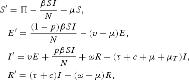 $$\eqalign{S^{\prime} & = \Pi - \displaystyle{{\beta SI} \over N} - \mu S, \cr & E^{\prime} = \displaystyle{{(1 - p)\beta SI} \over N} - (v + \mu )E, \cr & I^{\prime} = vE + \displaystyle{{\,p\beta SI} \over N} + \omega R - (\tau + c + \mu + \mu _T )I, \cr & R^{\prime} = (\tau + c)I - (\omega + \mu )R,} $$
with prevalence determined by I, force of infection (or ARTI) determined by pβSI/N, incidence of disease determined by vE+pβSI/N+ωR and case fatality determined by μ T I. Incidence of disease can be further split into primary or fast progression determined by pβSI/N, latent reactivation or slow progression determined by vE, and relapse progression determined by ωR.
The effective reproductive ratio for this model can be determined to be
 $$\eqalign{R_{\rm eff} & = \left( {\displaystyle{\beta \over {\mu + \mu _{\rm T} + c + \tau }}} \right)\left( {\,p + \displaystyle{{\left( {1 - p} \right)v} \over {v + \mu}}} \right) \cr & \times \left( {1 + \displaystyle{{\left( {\displaystyle{{\omega \left( {c + \tau} \right)} \over {\omega + \mu}}} \right)} \over {\left( {\left( {\mu + \mu _{\rm T} + c + \tau} \right) - \left( {\displaystyle{{\omega \left( {c + \tau} \right)} \over {\omega - \mu}}} \right)} \right)}}} \right).}$$
The endemic ratio of incidence to prevalence can be found by setting
 $$I^{\prime} {\rm = 0,}$$
and then
 $$\eqalign{& vE + \displaystyle{{\,p\beta SI} \over N} + \omega R - \left( {\tau + c + \mu + \mu _T} \right)I = 0, \cr & vE + \displaystyle{{\,p\beta SI} \over N} + \omega R = \left( {\tau + c + \mu + \mu _T} \right)I, \cr & \displaystyle{{vE + \displaystyle{{\,p \beta SI} \over N} + \omega R} \over I} = \tau + c + \mu + \mu _{\rm T}, \cr & \displaystyle{{\rm incidence} \over {\rm prevalence}} = \tau + c + \mu + \mu _{\rm T},} $$
Similarly the other ratios can be found to be
 $$\eqalign{& \displaystyle{{\rm incidence} \over {\rm mortality}} = \displaystyle{{\left( {\tau + c + \mu + \mu _{\rm T}} \right)} \over {\mu _{\rm T}}}, \cr & \displaystyle{{\rm incidence} \over {\rm ARTI}} = \displaystyle{{\left( {\tau + c + \mu + \mu _{\rm T}} \right)} \over \displaystyle{\beta / N}},} $$
Continuous introduction of treatment
We also explored the effect of parameter variation on the stabilization time of the ratio for the continuously improving treatment programme scenario (Fig. 4c ) using the same set of 1000 Latin Hypercube samples used to explore this variation in relation to the stepped scenario in the main text (Fig. 6). Under this scenario the distribution of stabilization times (as shown in Fig. 7) is about 2·5 times longer than in the stepped scenario but with all simulations stabilizing within 15 years of programme initiation.

Fig. 7. Shows the distribution of time to stabilize (in years) from Latin Hypercube sampling of 1000 samples during the continuous gradual introduction of a treatment programme of final τ = 2.
PRCC analysis
Table 2 shows the results of the PRCC analysis of the covariates for time taken to stabilize in the stepped scenario.
ACKNOWLEDGEMENTS
A. T. Newall holds an NHMRC Training Fellowship (630724, Australian Based Public Health Fellowship).
DECLARATION OF INTEREST
None.



