
INTRODUCTION
In sub-Saharan Africa (SSA), the rainfed agricultural sector is of the utmost importance. Currently it produces nearly 90% of SSA's food and feed and is likely to continue to do so (Rosegrant et al., Reference Rosegrant, Cai and Cline2002). It also provides the principal source of livelihood for nearly 70% of the human population in SSA, most of whom are amongst the poorest and most vulnerable communities in the continent. Added to the constraints imposed by extreme poverty and often a degrading resource base is the inherent risk caused by the within and between season variability of rainfall amounts and distribution. This variability poses challenges for farming communities who have to make investment decisions each year without a clear knowledge as to how the season will evolve and the yields they are likely to achieve. It is also a challenge for researchers who are seeking to identify innovations which will improve farm productivity whilst at the same time reduce climate-induced risk.
Dixit et al. (Reference Dixit, Cooper, Rao and Dimes2011) draw attention to the time constraints that often faces agronomic researchers who for a range of reasons may not be able to undertake their agronomic field research for more than three to four years. This relatively short time span raises the challenge of capturing the spectrum of rainfall variability that is likely to be experienced by farmers, and hence its impact on the longer-term performance of the innovation under investigation. In their paper, they illustrate how the use of complex crop growth simulation models such as the Agricultural Production Systems Simulator (APSIM) together with long-term climate data can help address this challenge. While such models arguably provide the most comprehensive approach to assessing the climate-induced risk associated with a wide range of soil and crop management options, they also require a great deal of detailed crop, soil and climate information as well as the necessary skills to use them effectively (Keating et al. Reference Keating, Carberry, Hammer, Probert, Robertson, Holzworth, Huth, Hargreaves, Meinke, Hochman, McLean, Verburg, Snow, Dimes, Silburn, Wang, Brown, Bristow, Asseng, Chapman, McCown, Freebairn and Smith2003).
Simpler rainfall analyses using long-term rainfall records can focus on the probability of events, or sequences of events, of known importance to farmers and their support agents. These include the start of the growing season, the frequency of dry spells within the season, the frequency of high intensity erosive rainfall events, the impact of prolonged wet spells on plant disease or the length of the growing season (Cooper et al., Reference Cooper, Dimes, Rao, Shapiro, Shiferaw and Twomlow2008). Such analyses are becoming increasingly easy to undertake as initiatives to provide more user-friendly software, and the training to go with it, take place. The outputs of such analyses are an adjunct to field-based agronomic research. They provide a useful framework for making medium-term strategic choices concerning agricultural practices that are directly influenced by single or a combination of climatic events as well as providing ex ante guidance to researchers in setting their priorities and in interpreting their results.
Various studies in the 1980s (e.g. Stern et al., Reference Stern, Dennett and Dale1982a, Sivakumar, Reference Sivakumar1988) described the importance of having access to long-term daily rainfall records to enable such analyses to be tailored to the needs of different groups of users. Without access to such records, the probability of occurrence and impact of important weather events, or sequences or events, cannot be determined and hence the risk of success or failure of weather-dependent innovations over the longer term cannot be assessed.
More recently, the issue of possible changes in rainfall patterns associated with global warming has added a further dimension, emphasizing the need to also establish whether or not such changes are evident in the rainfall records. Without first confirming that no major changes have occurred in recent years, it could be misleading to use long-term records going back 50 to 60 years to help characterize the climate-induced risk that farmers face today.
In this paper we use an actual case study from Zambia with the objective of illustrating the use of new and user-friendly climate analysis software to undertake contrasting types of analyses that examine the following aspects of weather induced risk associated with the inter and intra-seasonal variability of rainfall amounts and distribution:
• First, using both monthly rainfall totals as well as daily rainfall values, we examine the evidence (or lack of it) for any clear trends in rainfall amounts or their distribution.
• Using a maize crop as an example, we then use daily rainfall values for the 89 years to illustrate a range of risk analyses that include the date of the start of the season, the probability of dry spells both following planting and those that might occur during flowering.
• We also illustrate how the risk of important crop diseases, such as root rot in beans and aflatoxin in groundnuts could be assessed when a knowledge of a likely ‘weather trigger’ of the disease is available.
• Having examined the probability of events triggered by individual or a sequence of rainfall events, we illustrate how a simple crop water satisfaction index can be used to assess the relative performances and suitability of crops of different durations.
• Finally, we illustrate a different analytical approach to rainfall risk analyses. In all of the above approaches, the daily data are first summarized and then modelled, but in this last approach, the ‘order’ is reversed by first fitting a model to the daily data and then deriving risk analyses results from the fitted model.
The results presented focus solely on the analyses and use of rainfall data. We emphasize that this is not to dismiss the reality of the widely documented increasing temperatures (e.g. IPCC., 2007, Van de Steeg et al., Reference Van de Steeg, Herrero, Kinyagi, Thornton, Rao, Stern and Cooper2009) and the impacts that this may have in the longer term, especially on crop performance and, indeed, crop and variety choice (Cooper et al., Reference Cooper, Rao, Singh, Dimes, Traore, Rao, Dixit and Twomlow2009). However, whilst such increases are real, they are currently small. In addition, for rainfed agriculture, season to season variability in rainfall and possible changes in the pattern and in the variability are likely to be of more immediate concern to farmers.
MATERIALS AND METHODS
The case study context
This study uses data from Moorings Station in southern Zambia to illustrate appropriate methods of analysis. The issue in Zambia was that farmers were emigrating from southern Zambia, citing climate change as the reason they could no longer farm as they used to. A local non-governmental organization (NGO) accepted the evidence for climate change in temperatures and that farming in southern Zambia is risky, because of rainfall variability. But it was of the view that the evidence for change in the pattern of rainfall, and hence for different farming practices, was not so clear. The analysis in Zambia was just of rainfall data and the principal station used was Moorings (27.32°E; 16.15°S).
The source of the data
The daily data for Moorings were initially from February 1922 to early 2004. They were provided by the Zambia Meteorological Department. They were complete to the 1950s, but the later years had some gaps. Fortunately the Moorings Farm had a complete record since the 1950s, though they did not have the daily records for the early years. They also provided a file with monthly totals that had been computerized separately, i.e. the daily records had been totalled ‘by hand’ and the monthly totals then computerized. The existence of the monthly totals helped greatly in the checking process, described in Kurji et al. (Reference Kurji, Nanja, Stern and Rowlands2006). The checked and now complete data were shared with the Moorings Farm and the Zambia Meteorological Department, who have since provided the updated values to June 2010. The time needed to collect and check this daily data set was considerable. It is a step we find is often needed.
Analysing the monthly total for possible trends
The first set of analyses used monthly summaries. June to September is usually completely dry, so the analyses were for the eight months from October to May. The summary that is usually provided is the total rainfall for each month. This was plotted and ordinary linear regression models were fitted with the monthly totals as the dependent variable and the year as the independent variable. A separate curve was fitted to the data for each month, but they were all fitted together to test for an interaction between the month and the trend. The interaction tests whether the trend is the same in each month.
Trends were fitted in two ways. The first used a polynomial trend, as far as cubic terms. The second was to use non-parametric spline functions of the same complexity as the polynomials. The software package used was Genstat (VSN International, 2010), but any other standard statistics package that includes powerful regression modelling could equally be used. In each case we chose the function that explained more of the variability.
Analysing the number of rain days for possible trends
In this analysis we examined both the number of rainy days per month and the rainfall amounts per rainy day. The daily data, from which the monthly totals are calculated, contains a mixture of zero values (dry days) plus those with rain. In all these cases it is usual to split the analysis into two parts. The first part is a study of the zeros, i.e. the days with no rain. The second part is to examine the non-zero values, here the rainfall amounts on rainy days.
One slight complication with the rainfall data is to define the threshold for rain. The smallest amounts recorded are 0.1 mm, and in some countries, including this record in the early years, the lower limit was 0.01 inches. Below this value, days could be recorded as having trace rainfall. The ideal would be to record all non-zero values, i.e. to set the limit as ‘trace and above’. However, we chose a slightly higher limit, and a rain day was defined as one with more than 0.85 mm. This seemingly arbitrary value avoids complications at sites that are inconsistent in their recording of very small rainfalls, and also helps overcome possible complications in the original use of inches and mm in the recordings.
The trend analysis for the number of rain days used the same regression methods as the monthly rainfall totals, except that a generalized linear model was used. The dependent variable was the number of rain days in the month and this was modelled as of binomial type as a fraction of the total number of days in the month.
Dividing the monthly total by the number of rainy days gives the mean rain per rain day. Other summaries of the amounts have to be calculated from the daily data and we also examined the median rainfall and the number of days with heavy rainfall, which we defined as 20 mm or more.
Weather-induced risk analyses
The simple statistics package, Instat (University of Reading, 2008) was used, as it has a climatic menu, designed to provide the summaries described below. Once the summaries have been calculated, then any statistics package may be used for the further analyses, i.e. to assess evidence of a trend in the starting dates, and to calculate risks. Both Instat and Genstat were used.
The start of the season
While monthly summaries are often supplied by meteorological services, they are rarely demanded by users. The next set of analyses therefore examined examples of summaries from the daily data, where the precise definition may be tailored to the needs of particular users. In this case, farmers had stated that the pattern of rainfall was changing in ways that affected their farming practices. The start of the season for cropping is one key event as are problems of long dry spells during the season. Hence these were produced and analysed.
One example was to define the date of the start of the season thus:
The first occasion from 15 November with 20 mm or more within a 3-day period and no dry spell exceeding 10 days in the following 30 days.
This approach defines a single date for the earliest possible successful planting each year. Hence the daily data are summarized to give a set of 89 values (one for each year). In addition we calculated the risk of post planting dry spells that might cause seedling death across a range of potential planting dates.
Dry spells during the flowering period of maize
Dry spells occur during any rainy season in SSA and dry spells during flowering are an especially critical event for most crops. Maize is the mostly widely grown crop in Zambia, and farmers close to Moorings advised us that that flowering usually starts about 65 days post planting and extends over a 20-day window for the 125-day variety that they plant. To examine the risk of drought during flowering we looked at the probability of dry spells during the flowering period across a range of possible planting dates.
The risk of root rot in beans
Farrow et al. (Reference Farrow, Musoni, Cook and Buruchara2011) considered heavy rainfall events that may correspond to the development of risk of root rot disease in beans. Here we used the same definition of planting as described above, namely the first occasion with more than 20 mm in a three-day period and no dry spell exceeding 10 days in the next 30 days. Then after a two-and-half week period to account for germination and seedling establishment, taken as day 17, a high rainfall of more than 50 mm in a two-day period in the next 21 days was taken as a possible trigger for the bean root rot. A more stringent criterion was of more than 100 mm in a three-day spell.
The risk of aflatoxin in groundnuts
The second crop disease example was of the type of event that might lead to a season in which groundnuts had a high risk of aflatoxin. Terminal drought periods can greatly exacerbate aflatoxin infestation of groundnut pods (Hill et al., Reference Hill, Blankenship, Cole and Sanders1983; Wilson and Stansell, Reference Wilson and Stansell1983). For a 120-day groundnut variety this was taken to be a drought period in the last 30 days. This would cause the pod casing to dry and split, and hence allow access for the fungus. The event specified here was of less than 5 mm rain in any (running) 15-day period between days 90 and 120 following planting.
The crop water satisfaction index
The third set of results used a simple water balance index. Other papers in this issue (Dixit et al., Reference Dixit, Cooper, Rao and Dimes2011; Rao et al., Reference Rao, Ndegwa, Kizito and Oyoo2011) use a comprehensive crop model, APSIM, to investigate the integrated effects of variable rainfall, temperature and solar radiation on crop growth and yield under contrasting crop management options However, such models require substantial weather, crop and soil data input and skill to use (Keating et al., Reference Keating, Carberry, Hammer, Probert, Robertson, Holzworth, Huth, Hargreaves, Meinke, Hochman, McLean, Verburg, Snow, Dimes, Silburn, Wang, Brown, Bristow, Asseng, Chapman, McCown, Freebairn and Smith2003). However, a simpler ‘water balance’ model is available that has been fully described by Frere and Popov (Reference Frere and Popov1986) and more recently by Brown (Reference Brown2008). It has been widely used in SSA, for example in Zimbabwe (Senay and Verdin, Reference Senay and Verdin2003) and Ethiopia (Verdin and Klaver, Reference Verdin and Klaver2002).
The model calculates a water balance from a knowledge of the water input (rainfall) and the crop evapotranspiration (Et).
Et is calculated according to the equation:
where: Eo = the average potential evaporation, either calculated using the Penman-Monteith formula or by assuming an appropriate value for the location under study.
Kc = a crop coefficient that is related to its leaf area development and thus its changing water demands at different stages of growth.
Table 1 gives the coefficients and durations for two alternative maize varieties, that have growing periods of 105 and 125 days.
Table 1. The crop coefficients (Kc) for two contrasting duration maize varieties (Allen et al., Reference Allen, Pereira, Raes and Smith1998).

The water balance throughout the life of the crop is related to a crop water satisfaction index (CWSI) which is set at 100 at the start of the season. If the rainfall is sufficient throughout the season, then the final CWSI remains at 100, and this would be a year with no water stress. When the rain is insufficient, the CWSI drops by an amount that is proportional to the water balance shortfall. This calculation also includes a measure of soil water-holding capacity since water stored in rooting depth of the soil profile will act as a buffer to the onset of stress. This might be as little as 60 mm for sandy soils and over 150 mm for deep clay soils. If the soil profile is ever full then any further rainfall is assumed lost to the crop, through runoff and deep percolation beyond the root zone.
Whilst the model is very simple it has the value that it is transparent, easy to use and flexible. In this paper we assume that only daily rainfall data are available and also assume a constant value for Eo of 5 mm d−1. We show how a simple ex ante investigation of the effects of maize maturity length (105 v. 125 days) and soil water-holding capacity (60 v. 100 v. 150 mm) can guide a researcher with regard to the need for more detailed investigations, either through more complex modelling or through field trials. We also looked at the effects of date of planting. In this analysis, the criterion for planting corresponded as closely as we could to the criterion some farmers close to Moorings told us that they used. They would plant in early November, but only if there was very high rainfall, which we took to be more than 40 mm in a three-day period. From 15 November this was relaxed to a total of 20 mm, and further reduced to 15 mm from 1 December. With this definition we found that there was always a planting opportunity by mid-December and this corresponded to the farmers’ stated practice.
A modelling approach to rainfall analyses
The key feature of all the methods described above is that the daily data are first summarized and then modelled. For example, the monthly analyses, first calculates the total rainfall or number of rain days, each month, and then analyses these totals. For each month, the analysis is of the 89 totals. Similarly the start of the rains calculates the starting date for each of the 89 years, and then processes these dates. The length of the data to process is simply the number of years of data.
The final analyses use a different approach. They reverse the order by first fitting a model to the pattern of rainfall on a daily basis, and then deriving results from the fitted model.
The model is in two parts, because of the zeros in the daily data. The first part is a model of the occurrence of rain. We described above how it is natural to look at the number of rainy days in the month. We now take this idea further and look at the chance of rain on each day of the year.
If there is no trend in the data then this type of analysis can proceed by first calculating the number of rain days for each day of the year. For example, 15 December had rain in 44 of the 88 years. Hence the proportion of rainy days was 0.5. A curve can be fitted to this chance of rain, using standard regression methods, e.g. Woolhiser and Pegram (Reference Woolhiser and Pegram1979), McCullagh and Nelder (Reference McCullagh and Nelder1989). The basic data are binary (rain or no-rain) hence the fitting uses standard generalised linear models.
If the data are left in their time-series order, a model can be fitted to the occurrence of rain that also permits the year number to be included in the model and hence allow for a test for a possible trend in the chance of rain. Thus we fit a regression model to the original binary data, using the daily series of roughly 89 (years) by 365 observations per year, i.e. 32 272 values. The model has two parts, one for the trend and the second for the seasonality. Splitting data into trend and seasonality is a standard feature of time-series analyses. There is however one important difference from the time series modelling described earlier. When the data were summarized, e.g. to give monthly totals, before fitting the model, there is no real reason to consider the serial correlations between the successive observations, because they are a year apart. Hence simple regression models were used. This is often not the case when modelling the daily data, because in many places, if a given day is rainy, the next day is more likely to be rainy also. Thus rainy spells have a tendency to continue. Similarly dry spells have a tendency to continue, e.g. Jones and Thornton, Reference Jones and Thornton2002. So, rather than modelling just the chance of rain, we model the chance of rain given the previous day is dry, i.e. the chance that a dry spell continues, and also the chance of rain given the previous day is rainy, i.e. the chance that a rain spell continues.
If just the previous day is considered, this is called a Markov chain model of order 1. If the trend is ignored, this implies that two curves are fitted to the data, one for the chance of rain after dry days (i.e. the chance that a dry spell does not continue) and the second for the chance of rain after rain (i.e. the chance that a rain spell does continue). If both the two previous days are considered, then the Markov chain model is of order 2, and so on.
For the Zambia data a Markov chain model of order one was adequate for the chance of rain continuing, but a second-order chain was needed when the previous days were dry. Hence three curves were fitted to the data.
This type of model is used within various climatic modelling packages such as MarkSim (Jones and Thornton, Reference Jones and Thornton2000). It has been described in many papers since Gabriel and Neumann (Reference Gabriel and Neumann1962), e.g. Gates and Tong (Reference Gates and Tong1976), Haan et al., (Reference Haan, Allen and Street1976), Woolhiser and Pegram (Reference Woolhiser and Pegram1979), Stern et al. (Reference Stern, Dennett and Dale1982b). Stern and Coe (Reference Stern and Coe1984) showed how results, such as the chance of a long dry spell, could be calculated from the model.
The data were fitted in their original time-series order to examine the evidence for trend in the data. The quantification of an El Niño effect was also examined. The El Niño is explained as follows:
‘The NINO3.4 SST index is sea surface temperature anomalies averaged over the region bounded by 5°N to 5°S and 170°W to 120°W in the eastern-central equatorial Pacific. It is one of several standard SST indices associated with the El Niño/Southern Oscillation (ENSO), but considered the one that is considered most closely correlated with the behavior of ENSOFootnote 1.’ (Source: unpublished correspondence with James Hansen, IRI, 2009.)
For the analysis, each year was categorized into one of three alternatives, as follows. The average temperature anomaly from November to January was taken to characterize each year. A year was defined as El Niño if this temperature anomaly was less than minus 1. It was defined as La Niña if the anomaly was more than plus 1 and ‘Ordinary’ otherwise. The data were then analysed separately for each of these three types of year.
The modelling of the daily data also permits the results calculated in the previous sections of this paper to be derived. Because the method makes fuller use of the data, it can be used with shorter records. To illustrate the potential equivalent dry-spell risks are also calculated, both from the full record and also based on a very short record, from 2004 to 2009.
RESULTS
Analysing monthly data for possible trends
To gain a broad overview of possible trends in rainfall patterns, we first looked at the monthly totals. The overall pattern is shown in Figure 1.

Figure 1. Monthly rainfall totals (mm) at Moorings, Zambia (1922–2010).
A visual inspection of the monthly totals in Figure 1 indicates four important points as follows:
i. This graph does not give any evidence, from the monthly rainfall data, of climate change that would suggest that farmers should be changing their farming practices. They may have to change their practices for other reasons, like declining soil fertility or changes in input and output markets, but not particularly because of a change in the pattern of rainfall.
ii. This lack of major change is also a first indication that the long records of data may be used to estimate the comparative probability of success of different cropping strategies through a range of rainfall-induced risk analyses.
iii. Climate change can either be a change in the average or a change in the variability. An increase in variability would imply that farmers now have more extremes to contend with, than was the case previously. In Figure 1 this would indicate that recent years are more variable than those previously. Neither a visual inspection of Figure 1 nor the calculation of the standard deviation of the data for three successive 30-year periods indicated this.
iv. Fitting a model to assess evidence for change, i.e. a trend, was not statistically significant.
The lack of evidence of a trend is either because there is no change or because the large variability makes it difficult to detect, even with the long record. The variability of the monthly totals is because of the variability in the number of days with rain and also the variability of the rainfall amounts on those days.
We therefore also examined the number of rain days per month. The results are given in Figure 2 which shows the number of rain days each month, together with fitted curves. The chance of rain has not remained constant over the 89 years. The fitted curves are not straight lines, and a spline was fitted with four degrees of freedom. This fitted better than a model with no trend (p < 0.001).

Figure 2. Monthly total number of rain days at Moorings, Zambia (1922–2010) with fitted curves.
There was no evidence that the trend was seasonally dependent, i.e. the fitted ‘curves’ shown in Figure 2 for each month, may be parallel. (The data are counts of rainy days and so were fitted to be parallel on a logit scale.) As the trend in the different months could be the same, Figure 3 shows the ‘trend’ more clearly for the total number of rain days in the main rainy season from December to April.

Figure 3. Number of rain days in the main season at Moorings, Zambia (1922–2009) with fitted curve.
The trend is highly non-linear and this has important implications. In Zambia and elsewhere in SSA, many stations opened between 1950 and 1960. Hence analyses a few years ago, for example for the years 1950 to 2000, might have seemed to indicate a decrease in rainfall. However, when records available are as long as those for Moorings, the situation is seen to be more complex. The recent trend in Figure 3, is also upwards, not indicating the decrease that is sometimes claimed by farmers.
The monthly summaries of the rainfall amounts per rain day were also assessed for a trend. From the monthly analyses, i.e. the equivalent of Figure 2, there was some indication, though not conclusive, of a change (p = 0.015) with the mean rain per rain day, rising slightly over the past 40 years. The very large variability in rainfall amounts per rain day meant that this trend was not detectable when analysing on an annual basis, i.e. the equivalent of Figure 3.
The main messages, from Figure 1 to Figure 3, are first that any trend in the pattern of rainfall, from the monthly data, is not a simple one. Second, shown most clearly in Figure 1, is that almost all the variability in rainfall is inter-annual. Rainfall is extremely variable from year to year, and the cropping systems have to be able to cope with this variability. Third is that the large year-to-year variation, and possible trends are not new. They constitute the variability farmers have always had to cope with over the years.
Given the importance of this inter-annual variability of rainfall combined with the observation that there does not appear to be clear evidence of directional changes in rainfall patterns, the remainder of the paper concentrates mainly on examples of rainfall risk analyses. However, time series graphs are included as a check that it is reasonable to use the full series to calculate these risks.
Weather-induced risk analyses
The start of the season and the risk of dry a spell following planting. The analyses above used the availability of the daily data to some extent in order to process the monthly number of rain days, and the mean rain per rain day, as well as the monthly total rainfall. However, there is much more that can be done with access to the daily records due to the fact that crops (and their management) are often sensitive to single or a combination of rainfall events at specific stages during the cropping cycle. Hence, with access to daily data, it is possible to tailor the analyses to specific situations that are of particular concern to farmers and researchers. For example, due to the investment required in seedbed preparation, seed purchase and planting, a widespread concern amongst farmers across Africa is the date of the start of the rains and hence when a successful planting can be achieved. In many countries with a well-defined rainy season, there is considerable advantage to being able to plant early, but this opportunity has often to be offset because early planting might have a higher risk of being followed by a long dry spell resulting in seedling death and the need to re-plant. Farmers will be influenced by several factors in deciding when the rains have started. Amongst these will be their own degree of risk aversion, the frequency and amounts of early rainfall events as well as the texture of their soil which will determine how deep any sequence of rainfall events will penetrate and be stored in the soil. Clearly, even within any given village, there will be variability in farmers’ objectives and the soils they farm. These must be understood for any analyses to be of use.
As an example, Figure 4 shows the date of the start of the rains for one possible definition of the start of the rains. This is the first occasion, from 15 November that has at least 20 mm within a three-day period. However, this is combined with a second part of the definition: there should also not be a dry spell of more than 10 days in the 30 days following planting. With the inclusion of the dry-spell condition this might be termed a ‘successful planting date’ in that it identifies planting dates when a subsequent dry spell does not result in seedling death. Figure 4 thus shows the date when the first planting took place each year and in which of those years a dry spell occurred that necessitated re-planting. There are 12 such occasions, indicating a risk of not succeeding with early planting, i.e. possibly replanting, of 12/88, so about 14% or one year in seven.

Figure 4. Date of the start of the rain, at Moorings, Zambia (1922–2009).
Visually, from Figure 4, and from a simple regression analysis, there was no indication of a trend in the data, i.e. that planting dates had a tendency to be either later or earlier, in recent years.
If the dry spell following planting condition is changed to 12 days length, (not shown) then the risk dropped to 8 years in the 88, or about 9%. This indicates the improvement that might be achieved with a more drought-tolerant crop, or with simple moisture conservation measures such as soil surface mulching.
The results in Figure 4 provide the risk of seedling death from a given planting strategy that identified the earliest possible planting date each season, but not the risk from planting across a range of potential planting dates. This is shown in Figure 5 which gives the percentage of years that had a dry spell longer than 10, 12 or 15 days during the 30 days following planting dates ranging from mid October to the end of December conditional on the initial day being rainy. The top curve in Figure 5 shows that for a crop planted on 1 November, the risk is 45%, almost one year in two, of a dry spell of 10 days or more, sometime in November, i.e in the next 30 days. This risk is only about 15%, or one year in six, of a 15-day dry spell.

Figure 5. Dry spells following different planting dates at Moorings, Zambia (1922–2009).
By planting in mid-November the risk of a 10-day dry spell has halved, to one year in four, and shortly after the risk has reached a plateau. Hence someone wishing to minimize their risk could be advised to wait, if they were considering planting in early November, but there is no point in missing a planting opportunity from about 20 November, because the risk does not decrease further, but the chance of a damaging dry spell later in the season might increase. This possibility is examined in the next section.
Dry spells during the flowering period of maize. To examine the risk of drought during flowering, Figure 6 shows the percentage of years in which there is a long dry spell in successive 20-day periods. The results in Figure 6 are from an ‘unconditional’ analysis, i.e. there is no initial condition of rain, as there was in producing the results in Figure 5. Hence the risks in Figure 6 could include a dry spell that starts before the specified date and continues into the 20-day window. The result from Figure 6 is clear for Moorings: the risk of a long dry spell during the 20-day flowering period can never be discounted, i.e. no curve drops to zero, but the risk remains roughly constant until the end of January, in other words it remains roughly constant for crops planted up until about the end of November. For maize planted later during December and onwards and which flowers from early February onwards, the risk of a dry spell during flowering increases substantially. Reference to Figure 4 suggests that planting may not occur until early December (or later) in about 30 out of the 88 seasons, so moisture stress during flowering is certainly an issue to be considered at Moorings.

Figure 6. Percentage of years at Moorings, Zambia with a long dry spell during January to March.
Risk of root rots in beans. Figure 7 shows the maximum two-day and three-day totals for each year during the 21-day early growth period of beans as specified earlier in the methods section. From these data, Table 2 shows almost half the years (45%) had a two-day rainfall with more than 50 mm, but just one year in 10 had a three-day total of more than 100 mm. The values of 50 mm and 100 mm are relatively arbitrary, and Table 2 also shows how these risks change with a different threshold. For example changing the 50 mm value to 40 mm changes the risk to about 7 years in 10.
Table 2. Percentage of years at Moorings, Zambia with rainfall greater than a given threshold during the three-week period that could be sensitive for bean root rot.

Values in bold correspond to the thresholds used by Farrow et al., Reference Farrow, Musoni, Cook and Buruchara2011.

Figure 7. Maximum two and three-day total rainfalls at Moorings, Zambia from criteria in Farrow et al., Reference Farrow, Musoni, Cook and Buruchara2011) that indicate possible bean root rot infestation.
Given that root rot disease in beans can completely wipe out the crop in seasons of severe infestation (Farrow et al., Reference Farrow, Musoni, Cook and Buruchara2011), this analysis would suggest that detailed studies aimed at more clearly identifying rainfall threshold values should be considered in locations surrounding Moorings.
The risk of aflatoxin in groundnut. This and the root rot problem both lend themselves to either an ‘unconditional’ or a ‘conditional’ analysis. The conditional analysis calculates the risk, conditional on planting on a specific date. This can be done for a series of potential planting dates. The calculated risks then compare the risks for the different possible planting dates at a given site. This is illustrated in Figure 8 for the aflatoxin problem.

Figure 8. Risk of late season dry spells that could cause aflatoxin in groundnuts at Moorings, Zambia.
The result shows that the risk of the trigger event (less than 5 mm in any 15-day period, within the last 30 days of crop growth, i.e. 90 days post planting for this 120-day variety) is about 0.2, or one year in five, if the 90th day is in mid-February, i.e. if planting was by about 20 November. A delay of planting, by one month, increases the risk of this event to about four years in five. The same increase in risk would be caused if a longer season variety were used. As in the analysis for the risk of dry spells following planting (Figure 5) and the risk of dry spells during flowering in maize (Figure 6), this analysis suggests that planting crops towards the end of November around Moorings balances the risk of crop damage caused by both early and later dry spells.
The crop water satisfaction index
In this section, we examine how the distribution and amounts of rainfall in each of the full 88 seasons can be related to the crop water requirements of maize grown at Moorings through a simple water balance model as described earlier. Table 3 gives the values of the final CWSI for the 88 years at Moorings for an early planted 125-day maize variety. The ‘farmer derived’ criteria for planting, described earlier, were used to identify the earliest planting date in these analyses. The results indicate the sensitivity of the index to the water-holding capacity. With a soil of 60 mm water-holding capacity there are just eight years where the index remained at 100, i.e. no water stress occurred, with just under half the years having a final index of over 90. In contrast, with a soil of high water-holding capacity of 150 mm, over half the years had an index of 100, and all but 14 years, i.e. 85% of the years had a final index of over 90.
Table 3. Frequencies of water satisfaction index for 125-day maize grown at Moorings, Zambia.

While farmers have relatively little choice of the soil, they are able to choose what is cultivated on any particular soil type. Given the few years that a farmer with a soil of 60 mm water-holding capacity (either a sandy soil or a heavier textured but shallow soil) has a high index, we then examined whether such a farmer might benefit from considering a shorter-season variety. The results in Figure 9 compare the index for the 125-day variety with the values for a 105-day maize. The results indicate that the shorter-season variety usually, but not always, has a higher index. With the 105-day variety there are now 15 years (compared to eight for the 125-day crop) with a final index of 100. This is one year in five for the shorter crop, compared to one in ten for the 125-day maize. There were 69, i.e. four years in five, (compared to 57 for the 125 day crop) with an index of over 80. Note that visually from this graph, and a simple regression analysis, again do not show any evidence for a trend in the relative values of the two maturity types that would indicate a change in the seasonal pattern of rainfall through the record.
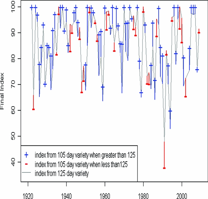
Figure 9. Crop water satisfaction index at Moorings, Zambia for two varieties of maize. (Joined line is for a 125-day crop and vertical lines are for a 105-day crop).
A tentative conclusion from Figure 9 is that the benefits from the risk reduction with the shorter-season variety of maize are evident but not large. Note that the index of 100 means that the crop has reached its full yield potential on the assumption that no other factors such as weeds or nutrients are limiting. However this yield potential will usually be higher for a longer-season maize. So a farmer should only switch to the shorter variety with a lower potential yield if it substantially reduces the risk. This does not seem apparent for the example considered. Although the CWSI is not an index of yield directly, a lower index generally implies lower yield (Frere and Popov, Reference Frere and Popov1986.)
Table 4 compares the final CWSI of a 105-day variety to that of a 125-day variety of maize, for different dates of planting that were achieved according to the planting rules used in the analyses above. The index is defined as similar when it is within two units. Overall the index is larger for the 105-day variety in about half the years, and smaller in about a quarter.
Table 4. Relative value of index for 105-day maize compared to 125-day variety at Moorings, Zambia.

In Table 4 one feature is that the comparative advantage of the 105-day variety seems less for the early planting. This is disappointing, because the early planting opportunity for the short-season crop reaches maturity in February and permits the possibility of planting a second legume crop. Examination of the data for individual years confirms that the occasional increased risk for the short-season crop is due to the larger water requirement for that variety in December (see Table 1) when dry spells can still be an issue at Moorings.
These, and the more complex crop models, can also be used as early warning indicators. This analysis takes the conditional risk ideas related to early planting above (Table 4), a step further. For example, suppose planting of the 125-day maize in the current year took place on 15 November and the index was still at 100 after 77 days, i.e. at the end of January. The results in Table 5 show the estimated values of the final index for two different levels of available soil water still in the profile. The soil water-holding capacity was taken as 100 mm.
Table 5. Frequencies of the final CWSI at Moorings, Zambia for 125-day maize planted on 15 November with different soil water contents on 31 January.

If the soil profile was full (last column in Table 5) then 76 out of 87 years, i.e. close to 90% would have had a final index of 95 or higher, promising an excellent chance of a good harvest. In contrast, with a half full profile, only 58 out of 87 years (66%) would have a final index of 95 or greater, which might be a cause for concern.
A modelling approach
One difficulty with the rainfall analyses, so far, is that the large inter-annual variation means that a long record is needed to estimate risks well or to investigate climate change.
Thus the lack of evidence for change in the pattern of the monthly rainfall totals, apparent in Figure 1, despite the long record, is either because there is not yet a clear picture, or because the picture is hidden, due to the large inter-annual variability. Figures 2 and 3 showed the picture was clarified by breaking the analyses of the rainfall totals into the number of rain days in the month, and the mean rain per rain day. This topic is investigated further in this section by using a more ‘sensitive’, i.e. more precise, method of analysis of the rainfall data, that would therefore have a chance of detecting smaller changes in the pattern of rainfall.
The analyses in the previous sections have always first summarized the daily data, and then processed the resulting summaries. Here we reverse the process. The first stage is to fit a model to the pattern of rainfall, using the daily data themselves. Then results are derived, from the resulting model.
The model is in two parts. The first is shown in Figure 10 and is a model for the chance of rain. There are three curves, because the chance of rain depends on whether the previous day had rain or was dry.

Figure 10. The estimated chance of rain following a rainy day (top curve), a single dry day (middle curve) and a dry spell of two or more days (bottom curve).
The top curve in Figure 10 is the chance of rain when the previous day also had rain. This is therefore the chance that a rainy spell continues for a further day. In January, the middle of the rainy season, this is over 0.6, i.e. about 2/3 of rainy days continued and had rain on the next day.
The bottom curve in Figure 10 shows the chance of rain after a dry spell of two or more days. This is therefore the chance that a dry spell (of longer than one day) is broken. This is a smaller probability than the chance of a rain spell continuing, rising to about 1/3 in January. The middle curve in Figure 10 is the chance of rain if yesterday was dry, but the day before that was rainy, i.e. the chance of rain after a single dry day. The difference between this curve and the bottom curve shows that then the chance of rain ‘returning’ is greater after just a single dry day, than if a dry spell has been in force for two days or more.
The model that has been fitted to the chance of rain might therefore be thought of as having a ‘memory’ of two days, if the previous day is dry. This is called a second-order Markov chain. The ‘memory’ is only a single day if the previous day had rain.
When there is rain, the rainfall amounts on a rainy day have a mean that is estimated by the curve shown in Figure 11. The mean rain per rain day is over 12 mm in the peak of the rainy season. Rainfall amounts are very variable and are usually modelled by a gamma distribution. The second parameter, i.e. the ‘shape’ parameter of the gamma is also needed to derive results from the model.
Figure 11. The mean rain per rain day (mm).
The models fitted in Figure 10 and Figure 11 have used all the daily data in the climatic record for Moorings. If this model is appropriate it can now be used to calculate any of the same ‘events’, such as the start of the rains, and risk of dry spells, that have been modelled in the previous sections. For simple events, such as the risk of a long dry spell, results can be calculated probabilistically as described in Stern and Coe (Reference Stern1984). Otherwise simulation (of many years) is used, as for example by Marksim (Jones and Thornton, Reference Jones and Thornton2000).
As an example, Figure 12 shows the chance of a long dry spell in the 30 days following a potential planting date. This is estimating the same characteristics as shown using the simple methods of analysis in Figure 5. The results are similar though the results from the Markov chain model slightly underestimate the risks as the season progresses.

Figure 12. Dry spell following planting, from Markov chain model to data from Moorings, Zambia (1922–2009).
One benefit from the modelling approach is that it can be used on shorter records than is possible with the simple methods of analysis. As an extreme example the same Markov chain model was fitted to just the last six years of data at Moorings (2004–2009). The results from fitting this model (not shown) were similar to Figure 10 but the lowest curve, i.e. the chance of rain given the two previous days were dry, was larger, i.e. close to a probability of 0.4 in January, compared to 0.3 for the full record. This implies a smaller risk of a long dry spell. In Figure 13 we present the same plot as Figure 12, but just derived from the last six years of data.

Figure 13. Dry spells as Figure 12, but based on data fitted only from 2004 to 2009.
For Moorings, with a long record, the extra precision from this modelling approach is of relatively little value, if climate change is ignored. The value of the method shown here is clearer when shorter records are all that are available, or when a record is split, to investigate climate change.
Here we illustrate splitting the record, by fitting a separate model to the data from El Niño years (17), La Niña years (13) and Ordinary years (58) identified in the record as described earlier.
As an example, we have taken the bottom curve from Figure 10 (the chance of rain following two or more dry days) and split it into three for the El Niño, Ordinary and La Niña years (Figure 14). There was no evidence of an interaction with the time of year, hence these curves are parallel. (The analysis was on the logit scale, so it is on this scale that the curves are parallel.) The difference, i.e. the need for three curves was statistically highly significant (p<0.001). The results in Figure 14 shows that the chance of a dry-spell being broken is considerably lower in El Niño years, compared to La Niña, with the Ordinary years being intermediate.

Figure 14. The estimated chance of rain after a dry-spell of two or more days, for El Niño, Ordinary and La Niña years.
The other curves in Figure 10 and the rainfall amounts were processed in a similar way. In summary, the El Niño effect was much less evident. Our conclusion for Moorings is that there is a clear El Niño effect. Rain spells are less likely to start in El Niño years, i.e. dry spells are longer. They are more likely in La Niña years than in Ordinary years. Once a rain spell starts then its duration and the rainfall amounts have essentially the same pattern for any of the types of years.
This type of result is of some relevance for the seasonal forecast, discussed in Hansen et al. (Reference Hansen, Mason, Sun and Tall2011). For example, for Moorings, if an El Niño year is expected, then estimates of the risk of planting, and of dry spells in the season, can use the appropriate model, and can provide a quantification of the effect of El Niño, etc., on any aspect of this risk demanded by farmers, e.g. start of the rains or of dry spells.
A further use of the modelling approach is to identify aspects of the pattern of rainfall that can then be studied further by the simpler approach to the analyses, described in previous sections of this paper. For example, further analysis of the bottom curve in Figure 14 (probability of rain after two or more dry days) did not imply an overall trend, but did indicate an interaction between the trend and the type of year. Hence the evidence for a trend in the data could be obscured by the El Niño effect, and a simple solution is to analyse the data, e.g. monthly totals, Figure 1 or number of rain days, Figure 3, for just the Ordinary years, i.e. omitting the El Niño and La Niña years.
As a second example, the largest El Niño effect in the model was of the bottom curve in Figure 10, which corresponds to the risk of a long dry spell. This effect was confirmed by calculating the length of the longest dry spell in the January to March period, split by the type of year. The longest spell in El Niño years averaged 14 days, compared with 12 in Ordinary years and just 10 days in La Niña years.
CONCLUSIONS
This paper is intended as an illustration of methods of analysis, rather than a report on the climatology of the Moorings station. One should always be cautious when reporting the results from any single station. Much of the work reported here was initially undertaken as an FAO-funded study for the conservation farming NGO. We were fortunate to work closely with the Zambia Meteorological Department and had full access to further stations from Southern Zambia to check the consistency of the results obtained.
Our examples focus on rain (the most commonly available data) because rainfall events are so important in rainfed agriculture and have an impact on a wide range of crop-related issues. However exactly the same kind of analyses can be done on other weather parameters (if the data is available) such as the risk of an impact of super-optimal temperatures during critical crop stages or the possible impact of low solar radiation levels, shown by Dixit et al. (Reference Dixit, Cooper, Rao and Dimes2011) to be important in influencing early maize growth at Kitale, Kenya.
The evidence for change in the pattern of rainfall is more complicated than the overwhelming evidence for rises in temperatures. This lack of solid evidence is clearly partly due to the very large inter-annual variability of the rainfall amounts, and hence the difficulty of detecting a small change.
We were fortunate to have 89 years data here, but 30–40 years of available data is more common and can be used in exactly the same way as we have shown. We have also shown that even shorter records can be usefully analysed using a Markov-chain type modelling approach. This is especially important if an initial analysis shows that there is indeed evidence of a change in weather patterns, and thus that there is a need to consider only more recent years, or just a particular type of year, e.g. El Nino years, in an analysis of climate induced risk.
However climate change is likely to continue for many years and we must therefore recognize that if, say, just the past 15 years are analysed as representing a ‘new state of affairs’, the change is likely to continue, so repeated monitoring and analyses at reasonable intervals may be needed.
There is much more that can be done. For example the monthly El Niño data from the International Research Institute for Climate and Society (IRI) is provided as a value that we have relatively arbitrarily categorized into three groups. It could, instead, be used as provided or categorized more finely.
The results from the Markov chain analyses also have possible implications for the data used in seasonal forecasting (see Hansen et al., Reference Hansen, Mason, Sun and Tall2011). The data usually used is the three-month rainfall totals. However the analysis above indicates that the El Niño effect (which forms part of the seasonal forecast, even if indirectly) is sometimes apparent through the changed risk of dry spells, and that rainfall totals on rainy days are largely unaffected. Hence there should be a better ‘signal’ if the rainfall event used is the number of rain days, or some function of dry spells, rather than the monthly rainfall totals. When using the totals, the rainfall amounts are likely to be adding unnecessary ‘noise’ to the data, and hence diluting the evidence for the forecast.
Lastly one must recognize that while the kind of ex ante analyses we have illustrated can help greatly in identifying and prioritizing field-based research, it merely provides an additional tool. It adds to, but does not replace the need for experimental and survey-based research, and for the many uses of detailed crop simulation models.
Acknowledgements
The initial analyses were for the NGO CFU (Conservation Farming Unit: www.conservationagriculture.org/CFU) who obtained funding from FAO for the original work. We are also very grateful to the staff from Moorings for their permission for their daily data to be made freely available, and to the staff from the Zambia Meteorological Department, for their help with the data and their collaboration, both in 2004 and more recently. We also acknowledge the contribution by the African Development Bank who partially funded this report through an ASARECA Project (No. FC-1–03) ‘Managing Uncertainty: Innovation Systems for Coping with Climate Variability and Change’.


 Open access