


Impact Statement
Cavitation and cavitation erosion are fundamental physical effects that limit the operating range and lifetime of hydraulic components and systems. For efficient development, it is necessary to make these complex phenomena accessible to virtual engineering. This research presents a computational fluid dynamics (CFD) model that significantly advances the understanding and simulation capability of cavitation erosion in oil hydraulic valves. Through the use of large eddy simulation (LES) turbulence modelling, careful parametrisation of cavitation models and cavitation erosion indices, this work addresses the challenges of simulating cavitation including vapour-gas separation and the influence of free air. The ability of this model to accurately reflect the location, shape and intensity of erosion, together with the damping effect of air, provides a practical tool for industrial use. It allows the engineer to identify, reduce or relocate erosion areas by optimising the flow path, thereby improving component performance. The model is validated by dozens of visualisations and four erosion experiments.
1. Introduction
The occurrence of cavitation in oil hydraulic components and systems is usually unavoidable and has a negative impact on the performance and service life of machines and systems. Particularly severe is the resulting cavitation erosion, which usually occurs in the most important hydraulic components such as pumps and valves (Weber & Gebhardt, Reference Weber and Gebhardt2020).
Cavitation represents the process of formation, oscillation and subsequent decay of cavities or bubbles within a liquid medium. In the context of mineral oil, which inherently contains a significant proportion of air, cavitation can be classified into three distinct types: vapour cavitation, gas cavitation and pseudo-cavitation. This classification is essential due to the unique physical processes underlying each type, leading to distinct causes and effects. Table 1 provides a comprehensive overview of these cavitation types along with their respective impacts.
Table 1. Types of cavitation in hydraulics
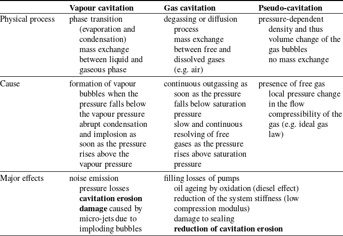
Vapour cavitation is a phase transition from liquid to gaseous state and vice versa analogous to boiling. However, the driving force here is not temperature, but pressure. If the local pressure drops below the vapour pressure, bubbles form. When these vapour bubbles enter areas of increased pressure, they condensate rapidly, causing an asymmetric bubble collapse near the wall, which creates a micro jet. This micro jet causes temporary and localised high mechanical stresses that lead to plastic deformations, crack initiation and grow up, which ultimately results in material loss. This process is called cavitation erosions and illustrated in figure 1. Cavitation erosion in hydraulic components is caused by vapour cavitation (Osterland et al. Reference Osterland, Müller and Weber2021).
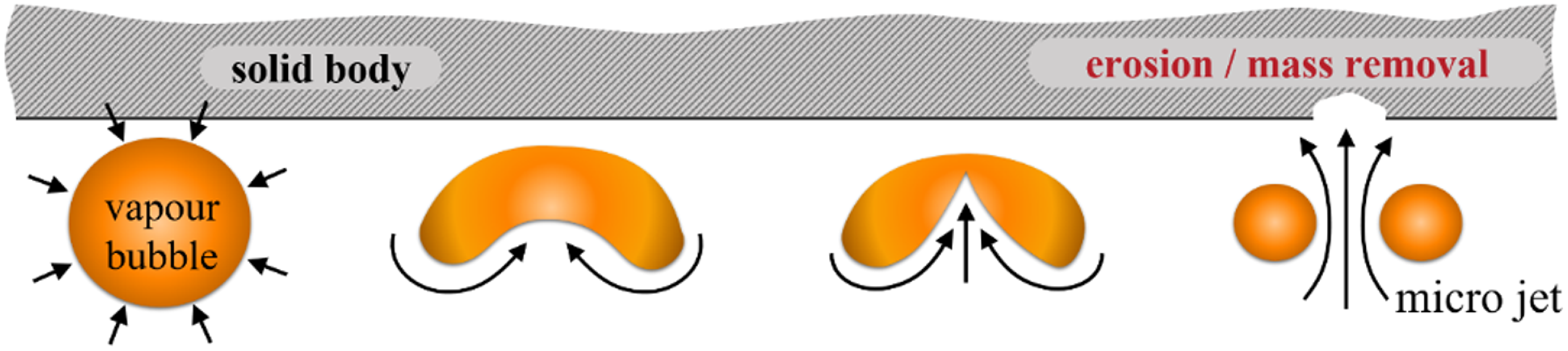
Figure 1. Process of cavitation erosion due to an asymmetrical vapour bubble collapse close to the wall.
In contrast to vapour cavitation, gas cavitation is not a phase transition. Instead, it is a process of diffusive outgassing or dissolution of gases within a liquid. The reduction of the local pressure below the saturation pressure leads to oversaturation of the liquid, which initiates a continuous outgassing process. Air bubbles exhibit a longer persistence compared with vapour bubbles and are conveyed along with the flow. These air bubbles undergo changes in their volume and density in response to the local pressure, a phenomenon referred to as pseudo cavitation since no further mass exchange takes place. The resolving of the free air is continuous and very slow compared with the condensation of the vapour bubbles, and depends on the bubble size, the pressure and flow conditions as well as the saturation state of the liquid. Gas and pseudo cavitation lead to filling losses in pumps, oil ageing and a reduced stiffness of the oil–air mixture. It is noteworthy that in a majority of hydraulic systems, all these types of cavitation coexist simultaneously and interact with each other.
The further development of hydraulic components and systems towards higher power densities and lifetimes is fundamentally challenged by the physical effects of cavitation and erosion. To minimise the negative effects of cavitation, it must be made accessible to numerical flow simulation to identify cavitation-related problems early on in the product development process and derive countermeasures. By means of computational fluid dynamics (CFD), it seems possible to optimise the flow guidance to reduce or relocate erosion areas. However, the correct simulative localisation of cavitation erosion in oil-hydraulic components has proven difficult in the past.
2. State of the art
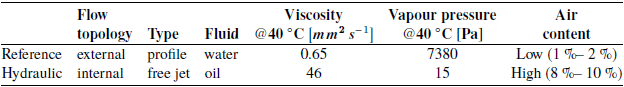
For the application of CFD under cavitating conditions, it is necessary to mathematically model the specific types of cavitation. In the literature, models for vapour cavitation such as those by Kunz (Reference Kunz2000) or Zwart, Gerber & Belamri (ZGB) (Reference Zwart, Gerber and Belamri2004), and for gas cavitation such as that by Lifante & Frank (Reference Lifante and Frank2008) are available. The complete cavitation model by Singhal et al. (Reference Singhal, Athavale, Li and Jiang2002) is, for example, used by Frosina et al. (Reference Frosina, Marinaro, Amoresano and Senatore2021) with default parametrisation to simulate cavitation in an oil-hydraulic spool valve. However, these models contain empirical parameters that were typically determined for water flowing around a profile. While it is in principle possible to apply these cavitation models to oil-hydraulic flows, the empirical constants must be re-determined and validated for mineral oil due to the significant differences in flow conditions and fluid properties, as shown in table 2.
Table 2. Reference flow in which most the cavitation models are parametrised versus oil hydraulic flow conditions
In the past, there have been attempts to apply models of vapour and gas cavitation to hydraulic flows. Frequently, the empirical constants within these models were modified to align the simulation with integral experimental results (such as pressure drop or volume flow) for one or a few operating points specific to the problem at hand. However, these methodologies resulted in vastly disparate parameter sets, with deviations of the order of 5000 % or even greater. Owing to the substantial uncertainty in the parametrisation of cavitation models for hydraulic oil, the predictive application of these models was constrained. Accordingly, the prediction of cavitation erosion was only possible to a limited extent and the influence of air on this was disputed. The following points are seen as reasons why the simulation of cavitation and cavitation erosion has not been successful so far:
-
• no clear separation between vapour and gas/pseudo-cavitation, although they differ in cause and effect;
-
• no direct, spatially resolved cavitation measurement, but indirect estimations via integral quantity such as pressures or volume flow rate;
-
• focus on individual operating points instead of the entire operating ranges;
-
• evaluation and comparison (sim. versus exp.) of momentary states, instead of statistic quantities;
-
• localisation and quantification of the cavitation load via volumetric gas fractions instead of cavitation erosion indices, although the areas at risk of cavitation erosion do not have to be identical to the areas of highest gas concentration;
-
• controversial influence of air on cavitation erosion in oil-hydraulic components.
By separating vapour and gas cavitation, the authors have achieved two important milestones on the field of cavitation in hydraulics in the recent past.
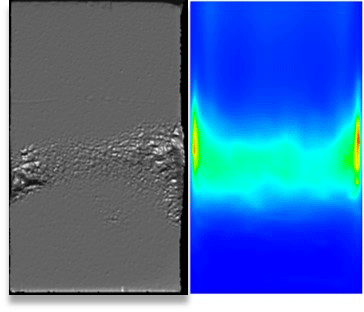
First, for a realistic valve flow, it was experimentally shown that air free mineral oil causes 4–5-times more mass loss ${\unicode[Arial]{x0394}} {m}$
than normal, saturated oil, see figure 2. This lead to the conclusion that ‘Cavitation erosion on hydraulic components like valves and pumps is caused by vapour cavitation – not gas or pseudo-cavitation’. In fact, the air released by gas cavitation reduces erosion significantly (Osterland et al. Reference Osterland, Müller and Weber2021).
${\unicode[Arial]{x0394}} {m}$
than normal, saturated oil, see figure 2. This lead to the conclusion that ‘Cavitation erosion on hydraulic components like valves and pumps is caused by vapour cavitation – not gas or pseudo-cavitation’. In fact, the air released by gas cavitation reduces erosion significantly (Osterland et al. Reference Osterland, Müller and Weber2021).
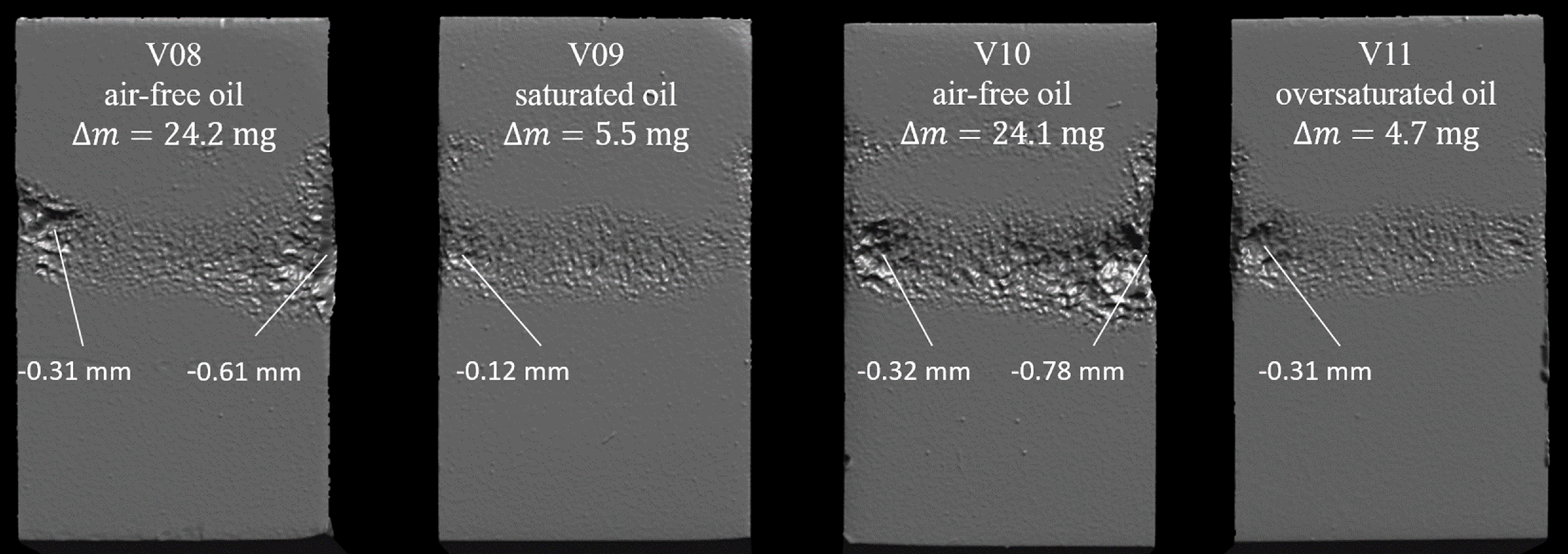
Figure 2. Three-dimensional surface scans of eroded samples, material, copper; fluid, HLP46; volume flow, $Q=97.5\,{\rm l}\,{\rm min}^{-1};$
pressure drop
$Q=97.5\,{\rm l}\,{\rm min}^{-1};$
pressure drop $\Delta p=145\,{\rm bar}$
; temperature
$\Delta p=145\,{\rm bar}$
; temperature $T=40\,^{\circ}\mathrm{C}$
; exposure time
$T=40\,^{\circ}\mathrm{C}$
; exposure time $t=5\,\mathrm{h}$
; details in Osterland, Müller & Weber (Reference Osterland, Müller and Weber2021).
$t=5\,\mathrm{h}$
; details in Osterland, Müller & Weber (Reference Osterland, Müller and Weber2021).
Second, Osterland et al. (Reference Osterland, Günther and Weber2022) succeeded in visualising the cavitating valve flow using a high-speed camera and the method of shadowgraphy. By using air-free mineral oil, it was possible to measure the spatial distribution of pure vapour cavitation for numerous operating points. Analogous experiments were carried out with normal saturated oil, in which vapour and gas cavitation occur. The experimental data is used to develop and parametrise a compressible Euler–Euler CFD model for mineral oil.
The comparison between Reynolds Averaged Navier–Stokes (RANS) simulations and large eddy simulations (LES) results showed that turbulence modelling has a very large influence.
Figure 3 compares the results of Menter’s (Reference Menter1994) shear-stress transport model (SST) and Nicoud’s (Reference Nicoud, Ducros and Poinot1999) wall-adapting local eddy-viscosity model (WALE) with experimental data, showing that RANS qualitatively predicts the vapour distribution incorrectly, while LES correctly reproduces the cavitation distribution. This shows a strong interaction between turbulence/vortices and cavitation, which is also seen experimentally in water by Lu et al. (Reference Lu, Zou and Fu2012). It is concluded that turbulence modelling with LES is necessary to simulate cavitation in hydraulic valves, because it resolves the momentary and local vortices and pressure field, which is essential to correctly calculate the cavitation distribution.
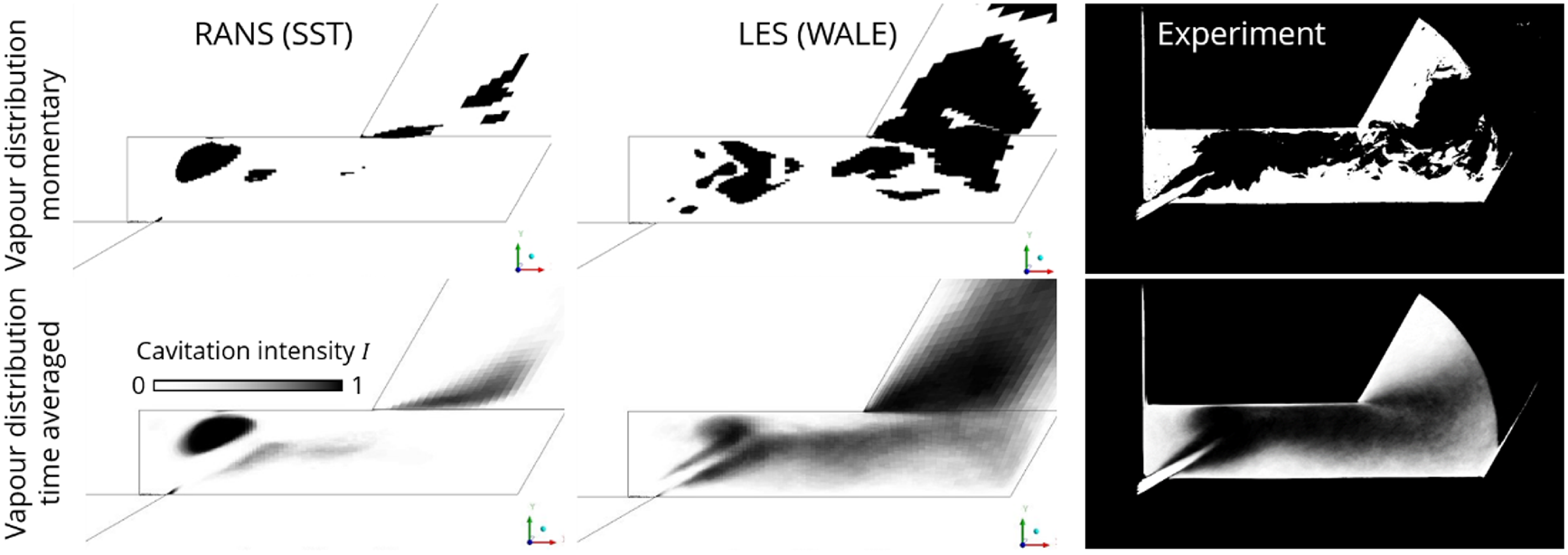
Figure 3. Influence of turbulence modelling on vapour distribution and comparison to experimental data (pure vapour cavitation ZGB model with standard parametrisation), (a) (time averaged) optical cavitation intensity details in Figures 6 and 10 of Osterland et al. (Reference Osterland, Günther and Weber2022).
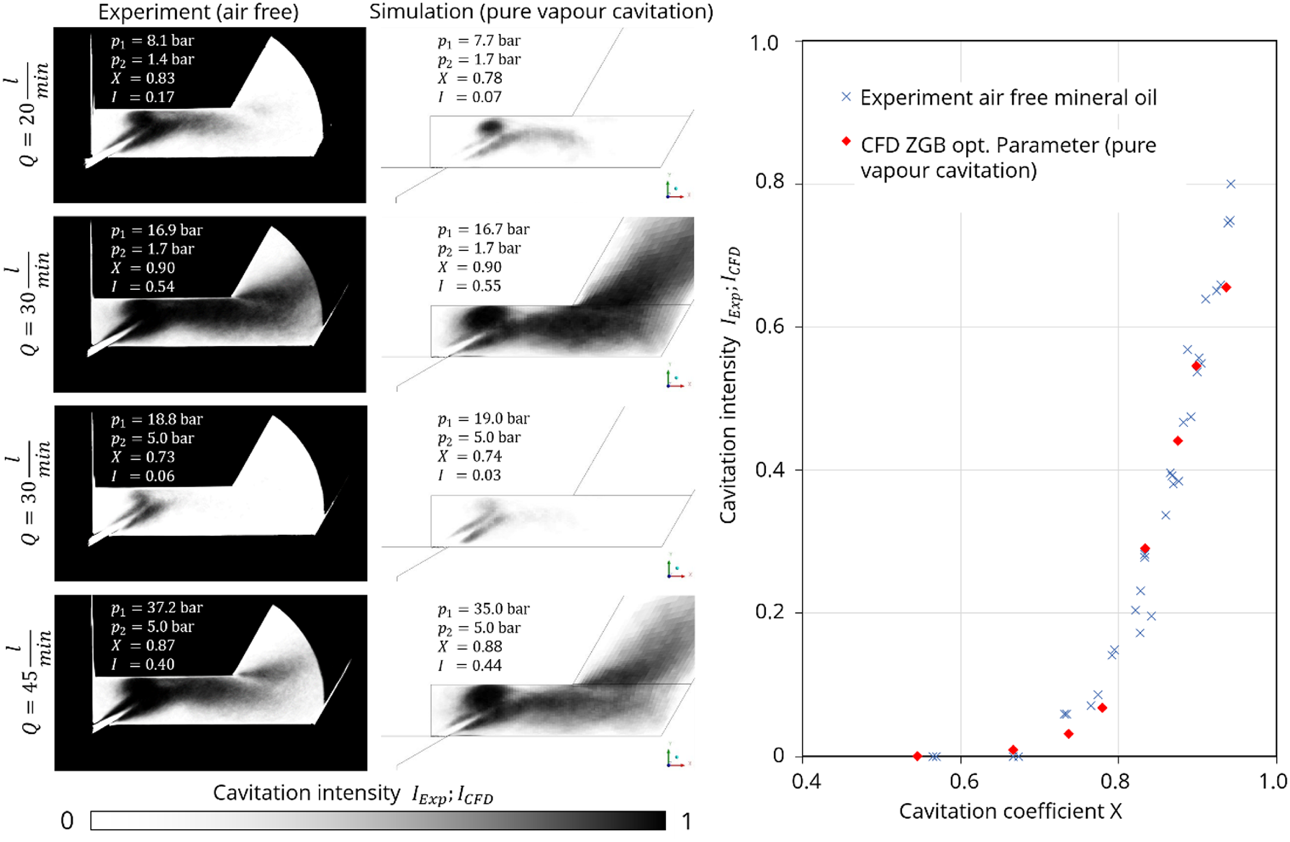
Figure 4. Comparison of spatial distribution and averaged cavitation intensities between air-free experiments and simulation with pure vapour cavitation with optimal parameters of the ZGB model for mineral oil, Osterland et al. (Reference Osterland, Günther and Weber2022).
The two empirical parameters of the ZGB model for vapour cavitation in mineral oil were determined. Figure 4 compares the measured optical cavitation intensity $I_{exp}$
of the air-free experiments with the simulated cavitation intensity
$I_{exp}$
of the air-free experiments with the simulated cavitation intensity $I_{CFD}$
. The results are plotted against the dimensionless cavitation coefficient
$I_{CFD}$
. The results are plotted against the dimensionless cavitation coefficient $X$
according to (1), where
$X$
according to (1), where $p_{1}$
is inlet pressure,
$p_{1}$
is inlet pressure, $p_{2}$
is the outlet pressure and
$p_{2}$
is the outlet pressure and $p_{v}$
is the vapour pressure of the fluid,
$p_{v}$
is the vapour pressure of the fluid,
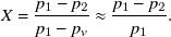 \begin{equation}X=\frac{p_{1}-p_{2}}{p_{1}-p_{v}}\approx \frac{p_{1}-p_{2}}{p_{1}}.\end{equation}
The comparison demonstrates that vapour cavitation in mineral oil can be simulated very well using LES turbulence modelling and the ZGB model with optimization parameters for oil, both in terms of spatial distribution and overall integration.
However, the gas cavitation model previously used showed its limitations, as it was not possible to correctly simulate very intensive and erosive operating points.
This paper overcomes the model limitations and extends the simulation methodology to localise and quantify cavitation erosion. Additionally, it depicts the damping influence of air on the cavitation erosion load.
3. Objective and procedure
The aim of this paper is the development and experimental validation of a simulations method for localising and quantifying cavitation erosion load in hydraulic valves using LES turbulence modelling and the cavitation erosion indices of Nohmi et al. (Reference Nohmi, Ikohagi and Iga2008).
On the experimental side, a test rig is briefly presented in which the air content can be freely adjusted and measured. Hence, it is possible to separate gas and vapour cavitation by completely degassing the fluid. The flow geometry is a transparent spool valve with optical access and removable erosions probe. The cavitating flow is visualised using a high-speed camera and the statistical shadowgraphy method for many different conditions and saturations.
On the simulation side, an Euler–Euler CFD model is presented, validated and applied to the erosive operating points used in figure 2. Due to the prior excellent results, the transport based ZGB model by Zwart et al. (Reference Zwart, Gerber and Belamri2004) with determined parameter for mineral oil is used for modelling the damage relevant vapour cavitation. To take the influence of air into account, an additional ‘oil–air’ phase is introduced. All phases are modelled compressible to reflect pseudo-cavitation. The simulation results of the spatial gas distribution are compared with the visualisation data, which show good agreement.
The model is then used to relatively quantify the cavitation erosion load under intense conditions. By comparing the simulation results with the damage pattern in figure 2, it is shown that the areas of maximum vapour concentration near the wall are not congruent with the observed erosion regions. Hence, the vapour volume fraction alone is not a suitable erosion indicator. In contrast to this, the cavitation indices by Nohmi succeed in reflecting the location, shape and intensity of cavitation erosion. Even local details such as the increased mass loss at the edges are reflected with high precision. The simulation is used to analyse this local effect, which lies in the formation of strong longitudinal vortices precisely at these points, which again show a strong coupling between turbulence/vortices and cavitation. The CFD model also reflects the experimentally observed damping effect of air.
4. Experimental set-up
Figure 5 shows the test rig for flow and cavitation visualisation as well as for erosion testing. It provides a unique combination of valuable features.
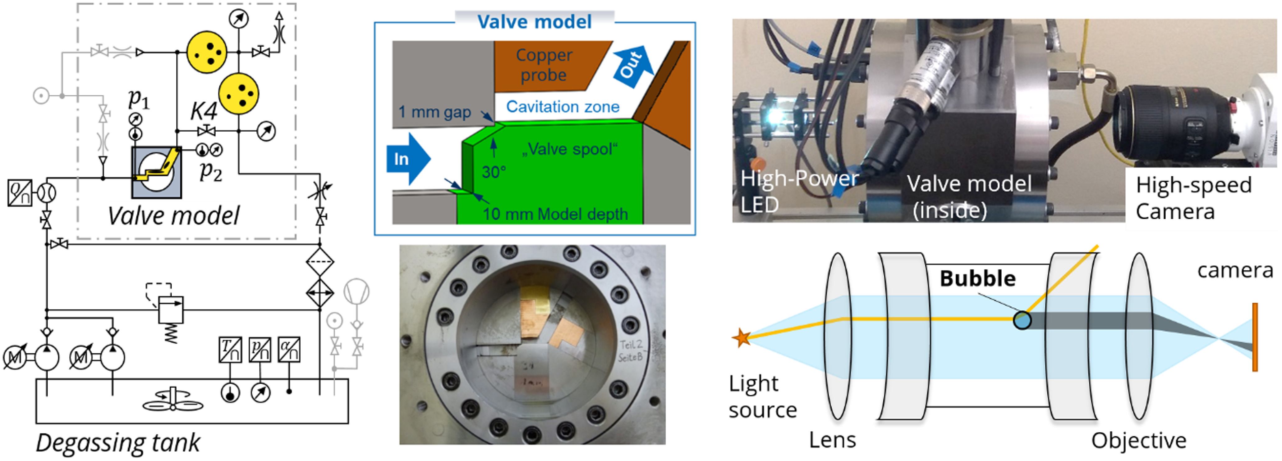
Figure 5. Hydraulic circuit diagram, flow geometry (spool valve) with erosion sample, optical set-up for flow visualisation and schematic representation of the shadowgraphy method with ray path and shadow cast on the camera by a gas bubble; details on the experimental set-up and procedure are found from Osterland (Reference Osterland2024).
Most important is the specially designed airtight hydraulic reservoir in which the air contain of the fluid can be adjusted and measured. By degassing the oil, it is possible to suppress gas cavitation completely, as there is neither free nor dissolved gas in the fluid. Consequently, only vapour cavitation can occur, which means that the cavitation types are clearly separated from each other.
As for flow geometry, the planar valve-like flow geometry shown in figure 5 is used. The benefit of this particular flow configuration is that it accurately mirrors the topology, dimensions and operating conditions found in actual valves. As a result, the emergent flow regime, characterised by velocities, pressures, turbulence and cavitation distribution, is a direct representation of real-world conditions. This ensures a very high transferability of the test results to real hydraulic components.
The flow geometry has an optical access through which the cavitation is visualised by a high-speed camera and the method of shadowgraphy. This technique is based on the refraction of light due to changes in the refractive index, which are induced by variations in the medium’s density. Shadowgraphy produces a high contrast, which depends on the density gradient, and thus shows a high sensitivity to the density discontinuity at the phase boundary of the gas bubbles. As a consequence, the gas bubbles cast a shadow in the image plane. The high-speed images are high-contrast filtered and averaged, with the grey scale corresponding to the mean bubble occurrence probability, see figure 6. The optical cavitation intensity $I$
is quantified by spatial averaging over the valve chamber. In this example, the cavitation in intensity is
$I$
is quantified by spatial averaging over the valve chamber. In this example, the cavitation in intensity is $I_{avg}=0.109$
, which means that on average 10.9 % of the valve chamber is black.
$I_{avg}=0.109$
, which means that on average 10.9 % of the valve chamber is black.

Figure 6. Shadowgraphy of pure vapour; original contrast and averaged image, operation point: $Q=20\,{\rm l}\,{\rm min}^{-1}, p_{1}=8.2\,{\rm bar}, p_{2}=1.7\,{\rm bar}$
, air-free oil.
$Q=20\,{\rm l}\,{\rm min}^{-1}, p_{1}=8.2\,{\rm bar}, p_{2}=1.7\,{\rm bar}$
, air-free oil.
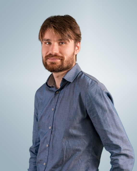
A total of 99 visualisation experiments were carried out in which the saturation, the inlet and outlet pressure or the volume flow Q were varied. The results are summarised in figure 7, where the optical cavitation intensity $I$
is plotted against the dimensionless cavitation coefficient
$I$
is plotted against the dimensionless cavitation coefficient $X$
.
$X$
.
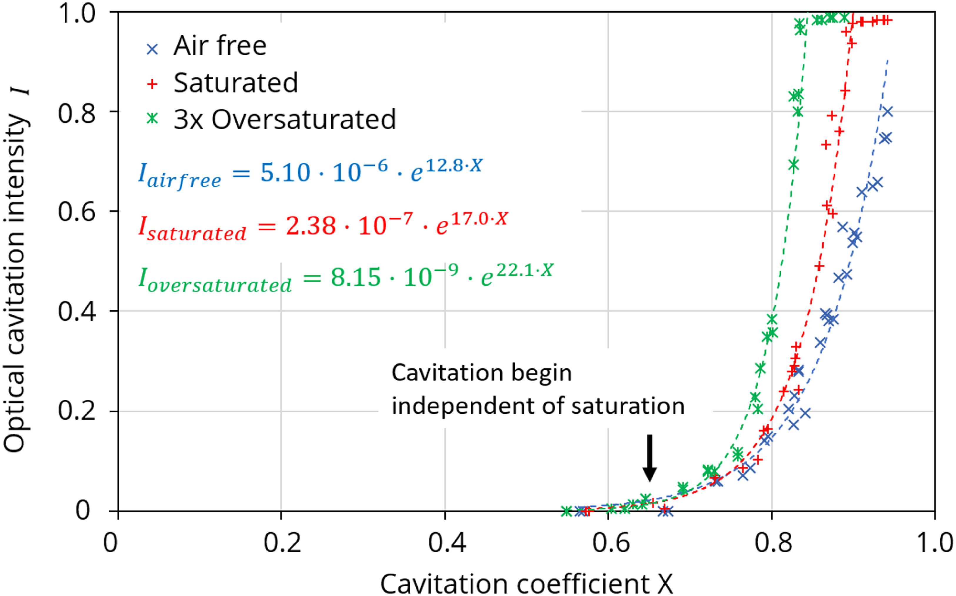
Figure 7. Cavitation intensity at different dissolved air contents above the cavitation coefficient X with fitting functions of the form $ae^{bX}$
.
$ae^{bX}$
.
It can be observed that the measurements for the same saturation follow a specific curve. Hence, the cavitation state in the valve is completely described by a parameter, e.g. $X$
. The results of the visualisation experiments form the basis for the parametrisation and validation of the cavitation models for mineral oil. The full set of the visualisation data can be found in Appendix A and discussed in more detail by Osterland et al. (Reference Osterland, Günther and Weber2022).
$X$
. The results of the visualisation experiments form the basis for the parametrisation and validation of the cavitation models for mineral oil. The full set of the visualisation data can be found in Appendix A and discussed in more detail by Osterland et al. (Reference Osterland, Günther and Weber2022).
Additionally, the test rig is used for erosion test. For this, a removable copper probe is mounted in the cavitation zone. A total of four five-hour-long erosions tests with different saturation levels were performed. The cavitation erosion is quantified by the mass loss during that exposure time. The results show a 4.4–5.1 higher mass loss when using air-free oil compared with saturated oil, as shown in figure 2. For erosion tests with saturated mineral oil, the amount of free air in the wake was roughly determined to be 5–20 % of the maximum soluble air, using a bubble analysis section. The results of the erosion test are used to validate the simulated cavitation erosion load. The fluid is a standard mineral oil HLP46 Fuchs Renolin B15 VG46 at a constant temperature of 40 °C.
5. CFD simulation
5.1 Meshing, basic settings and governing equations
In accordance with the experiment, the flow geometry shown in figure 8 consists of the valve chamber, and inlet and outlet sections, which minimise the influence of pressure boundary conditions and ensure a complete development of the flow and turbulence. The valve chamber and the walls are meshed in detail, as high velocity and density gradients, as well as turbulence and vortex production, are expected in these areas. The mesh is of high quality to minimise numerical divergences and computational costs.
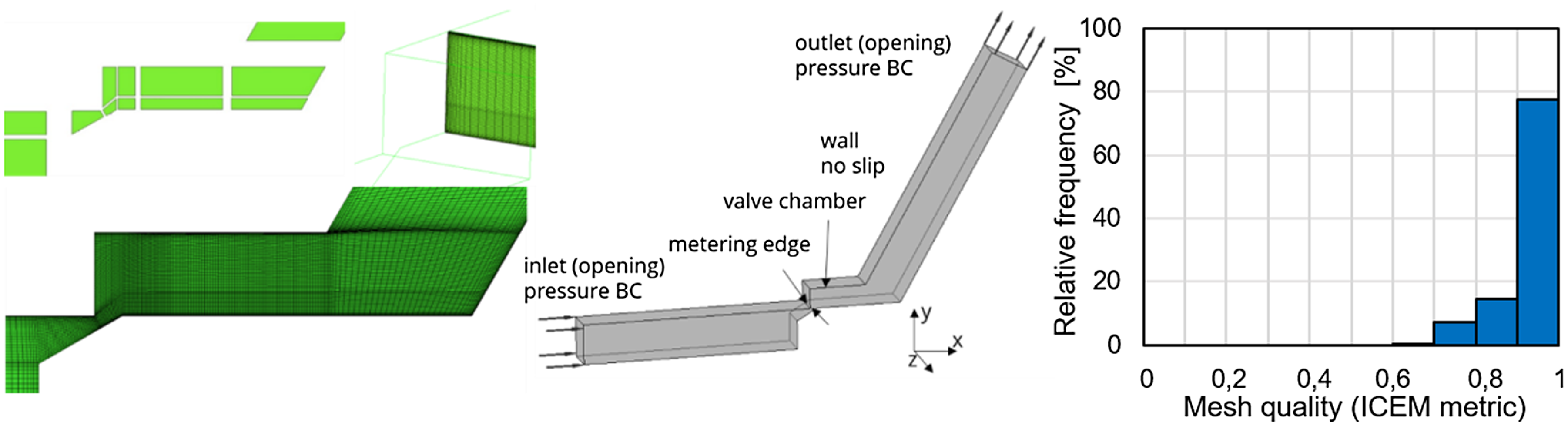
Figure 8. Flow geometry, mesh and boundary conditions (BC), and mesh quality; 615 000 Hex cells, $y^{+}\lt 1$
.
$y^{+}\lt 1$
.
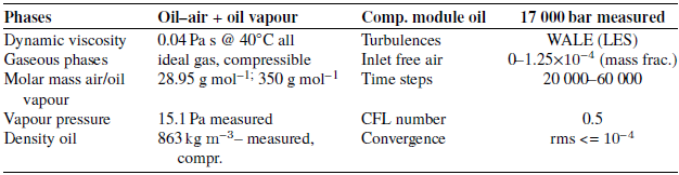
The fluid properties and basic numerical setting are summarised in table 3.
Table 3. Overview of the fluid properties and basic numerical setting
The multiphase flow is simulated using the isotherm homogeneous Euler–Euler method, in which all phases are assumed to possess identical pressure and velocity fields. In every cell each phase has a volumetric fraction $\alpha _{k} \epsilon [0,1]$
. In a finite volume, the sum of all volumetric fractions must equal one
$\alpha _{k} \epsilon [0,1]$
. In a finite volume, the sum of all volumetric fractions must equal one $(\sum \alpha _{k}=1)$
. For each phase, a continuity equation (2) is formulated, where
$(\sum \alpha _{k}=1)$
. For each phase, a continuity equation (2) is formulated, where $\alpha _{k}$
is the volume fraction of the phase k,
$\alpha _{k}$
is the volume fraction of the phase k, $\rho _{k}$
the density of the phase,
$\rho _{k}$
the density of the phase, $u_{i}$
the velocity and
$u_{i}$
the velocity and $S_{k}$
the source terms modelling the phase transition. Due to mass conservation, the sum of the sources have to be 0 (
$S_{k}$
the source terms modelling the phase transition. Due to mass conservation, the sum of the sources have to be 0 ( $\sum S_{k}=0)$
,
$\sum S_{k}=0)$
,
 \begin{equation}\frac{\partial \alpha _{k}\rho _{k}}{\partial t}+\frac{\partial \alpha _{k}\rho _{k}u_{i}}{\partial x_{i}}=S_{k}.\end{equation}
The conservation of momentum, neglecting of volumetric forces such as gravity, is given by
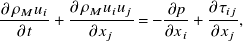 \begin{equation}\frac{\partial \rho _{M}u_{i}}{\partial t}+\frac{\partial \rho _{M}u_{i}u_{j}}{\partial x_{j}}=-\frac{\partial p}{\partial x_{i}}+\frac{\partial \tau _{ij}}{\partial x_{j}},\end{equation}
where $\tau _{ij}$
is the sheer stress tensor,
$\tau _{ij}$
is the sheer stress tensor, $\rho _{M}$
is the mixture density, which is calculated from the local volume fractions
$\rho _{M}$
is the mixture density, which is calculated from the local volume fractions $\alpha _{k}$
and their densities
$\alpha _{k}$
and their densities $\rho _{k}(p)$
according to (4). The densities of a phase
$\rho _{k}(p)$
according to (4). The densities of a phase $\rho _{k}$
is specified by an equation of state e.g. ideal gas law,
$\rho _{k}$
is specified by an equation of state e.g. ideal gas law,
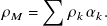 \begin{equation}\rho _{M}=\sum \rho _{k}\alpha _{k}.\end{equation}
The mixture viscosity $\eta _{M}$
of a gas–liquid mixture depends in a complex way on the specific operation conditions, flow form, number of bubbles and bubble spectrum, and is in general unknown, since it would require complex rheological measurements on gas/oil mixtures. Aung & Yuwono (Reference Aung and Yuwono2012) compared ten mixture viscosity models with experimental data, with the result that, with the exception of the Owen’s model (Reference Owen1961), all models are unsuitable for calculating the pressure drop of a gas–liquid mixture. The simple Owen model assumes the viscosity of the liquid for the mixture viscosity
$\eta _{M}$
of a gas–liquid mixture depends in a complex way on the specific operation conditions, flow form, number of bubbles and bubble spectrum, and is in general unknown, since it would require complex rheological measurements on gas/oil mixtures. Aung & Yuwono (Reference Aung and Yuwono2012) compared ten mixture viscosity models with experimental data, with the result that, with the exception of the Owen’s model (Reference Owen1961), all models are unsuitable for calculating the pressure drop of a gas–liquid mixture. The simple Owen model assumes the viscosity of the liquid for the mixture viscosity $\eta _{M}$
, see (5). Of course, this modelling assumption is a great simplification. Given the relatively high viscosity of mineral oil and the small geometry, viscosity modelling might interact with local shear rates and impact the vortices and hence the cavitation behaviour. However, the Owen model is at least equal to or better than other mixture viscosity models like the often used linear interpolation between gas/liquid as the programme’s default setting. In addition, the Owen model offers the advantages that the simplification is clearly known and named, and that additional and questionable viscosity gradients within the flow are avoided,
$\eta _{M}$
, see (5). Of course, this modelling assumption is a great simplification. Given the relatively high viscosity of mineral oil and the small geometry, viscosity modelling might interact with local shear rates and impact the vortices and hence the cavitation behaviour. However, the Owen model is at least equal to or better than other mixture viscosity models like the often used linear interpolation between gas/liquid as the programme’s default setting. In addition, the Owen model offers the advantages that the simplification is clearly known and named, and that additional and questionable viscosity gradients within the flow are avoided,
 \begin{equation}\eta _{M}=\eta _{oil}=\eta _{\textit{vapor}}=\eta _{air}=0.04\,\mathrm{Pas}.\end{equation}
To accurately represent the significant influence of vortices on cavitation, as shown in figure 3, turbulence is simulated using the wall-adapting local eddy viscosity (WALE) model by Nicoud et al. (Reference Nicoud, Ducros and Poinot1999), which uses the LES approach. Unlike the RANS method, the application of LES necessitates fine meshing, small time steps and extended periods for averaging, which cause relatively large computational resources. The software Ansys CFX is used and the computation is done on the local cluster Taurus at ZIH TU Dresden. On average, one simulation uses 128–256 CPUs and takes approximately 8 h.
5.2 Cavitation model
Due to the very good results, as already shown for pure vapour cavitation in figure 4, the damage relevant vapour cavitation is modelled by the transport-based ZGB model with the determined empirical parameter for mineral oil. The gaseous phase ‘oil vapour’ is modelled compressible using the isotherm ideal gas law. The phase transition (mass exchange) in the ZGB model is driven by the difference between the local pressure $p$
and the vapour pressure of the oil
$p$
and the vapour pressure of the oil $p_{v}$
. The modelling equations including the Osterland, Günther & Weber (2022)-determined empirical parameters
$p_{v}$
. The modelling equations including the Osterland, Günther & Weber (2022)-determined empirical parameters $C_{vap}$
and
$C_{vap}$
and $C_{cond}$
for mineral oil are given in (6)–(8). The vapour cavitation model is implemented manually via the CFX expression language as source terms
$C_{cond}$
for mineral oil are given in (6)–(8). The vapour cavitation model is implemented manually via the CFX expression language as source terms $S_{k}$
in corresponding continuity equations of the phases.
$S_{k}$
in corresponding continuity equations of the phases.
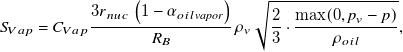 \begin{equation}S_{Vap}=C_{Vap}\frac{3r_{nuc}\left(1-\alpha _{oil\textit{vapor}}\right)}{R_{B}}\rho _{v} \sqrt{\frac{2}{3}\cdot \frac{\max (0,p_{v}-p)}{\rho _{oil}}},\end{equation}
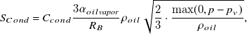 \begin{equation}S_{Cond}=C_{cond}\frac{3\alpha _{oil\textit{vapor}}}{R_{B}}\rho _{oil} \sqrt{\frac{2}{3}\cdot \frac{\max (0,p-p_{v})}{\rho _{oil}}},\end{equation}
with
 \begin{equation}C_{vap}=50;C_{cond}=10^{-4};r_{nuc}=5\cdot 10^{-4}, R_{B}=10^{-6}\mathrm{m}, p_{v}=15,1\,\mathrm{Pa}, \rho _{oil}=863\;\mathrm{kg}\,\mathrm{m}^{-3}.\end{equation}
In contrast to previous works, the complex Lifante gas cavitation model is abandoned due to its limitations, which do not permit the simulation of erosive operating points. To nevertheless represent the influence of air, it is assumed that the mass fraction of free air $r_{L}$
is constant and homogeneously distributed in the flow. This is modelled through the implementation of an ‘oil–air’ phase, which reduces the number of phases to two.
$r_{L}$
is constant and homogeneously distributed in the flow. This is modelled through the implementation of an ‘oil–air’ phase, which reduces the number of phases to two.
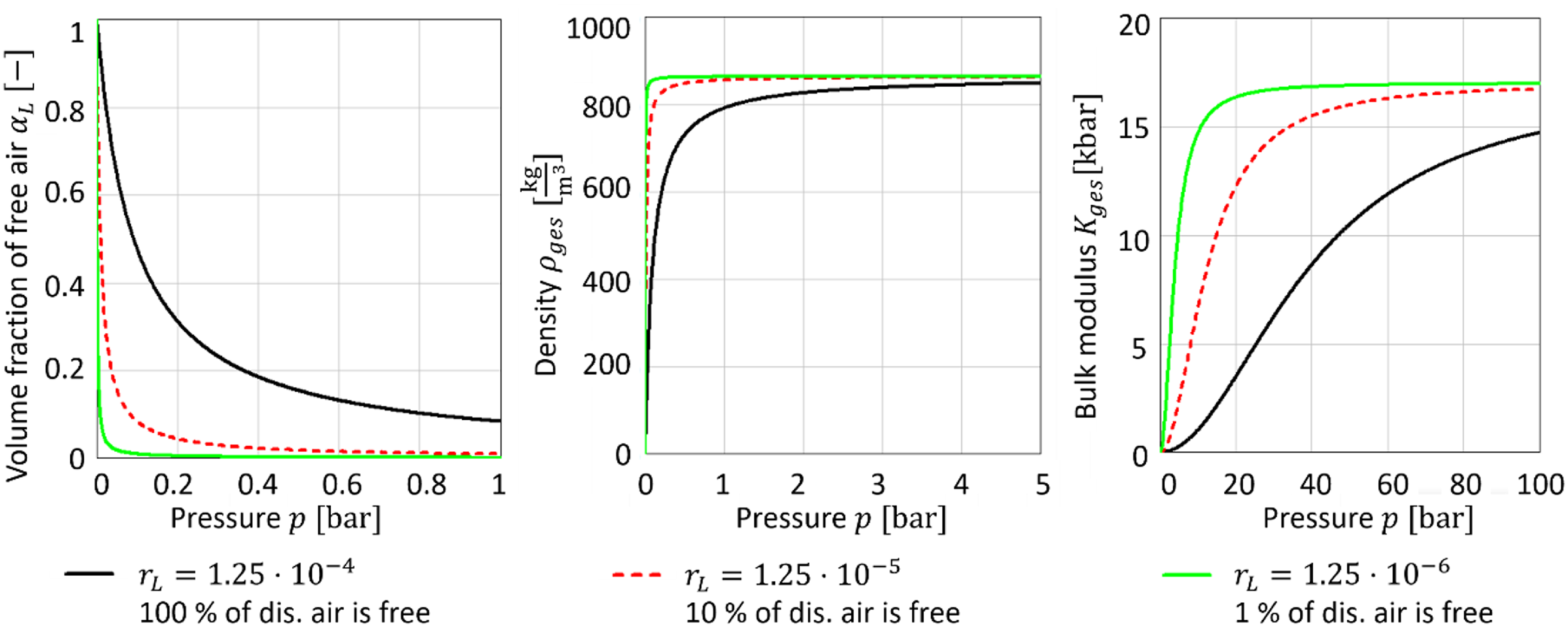
Figure 9. Properties of the oil–air mixture as a function of pressure for different mass fractions of free air; 100 % = all the dissolved air is present as free air.
The volume fraction of free air $\alpha _{L}(p,r_{L})$
, the density
$\alpha _{L}(p,r_{L})$
, the density $\rho _{ges}(p,r_{L})$
and the compression modulus
$\rho _{ges}(p,r_{L})$
and the compression modulus $K_{ges}(p,r_{L})$
of the oil–air mixture are calculated according to (9)–(12), which are illustrated in figure 9. These state equations assume an ideal mixture and isothermal conditions. Naturally, the behaviour of air in valve flow is adiabatic, but for the sake of simplification, the flow is modelled as isothermal. This is primarily because the major effect of free air is the increased compressibility, which is adequately captured in this model. While temperature does play a role, the effect of pressure is dominant.
$K_{ges}(p,r_{L})$
of the oil–air mixture are calculated according to (9)–(12), which are illustrated in figure 9. These state equations assume an ideal mixture and isothermal conditions. Naturally, the behaviour of air in valve flow is adiabatic, but for the sake of simplification, the flow is modelled as isothermal. This is primarily because the major effect of free air is the increased compressibility, which is adequately captured in this model. While temperature does play a role, the effect of pressure is dominant.
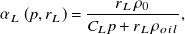 \begin{equation}\alpha _{L}\left(p,r_{L}\right)=\frac{r_{L}\rho _{0}}{C_{L}p+r_{L}\rho _{oil}},\end{equation}
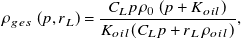 \begin{equation}\rho _{ges}\left(p,r_{L}\right)=\frac{C_{L}p\rho _{0}\left(p+K_{oil}\right)}{K_{oil}(C_{L}p+r_{L}\rho _{oil})},\end{equation}
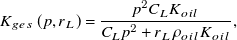 \begin{equation}K_{ges}\left(p,r_{L}\right)=\frac{p^{2}C_{L}K_{oil}}{C_{L}p^{2}+r_{L}\rho _{oil}K_{oil}},\end{equation}
with
 \begin{equation}\rho _{0}=1.184\,{\mathrm{kg}}\,{\mathrm{m}^{-3}};\ \rho _{oil}=863\,{\mathrm{kg}}\,{\mathrm{m}^{-3}};\ K_{oil}=17\,000\, \mathrm{bar};\ C_{L}=\frac{M_{L}}{RT_{abs}}=1.16\times 10^{-5}\,{\mathrm{s}^{2}}\,{\mathrm{m}^{-2}}.\end{equation}
A closer look at (9) reveals that it is a barotropic or equilibrium model for pseudo-cavitation, since the density of the air–oil mixture is only an algebraic function of the pressure and has no time or path dependencies, i.e. a change in pressure leads directly to a change in density. The equilibrium modelling does not lead to the often reported disadvantages, especially with regards to the cavitation location, because the damage-relevant vapour cavitation continues to be modelled with the inertial transport approach.
5.3 Post-processing using ‘virtual shadowgraphy’
Due to the Euler–Euler approach, only the concentration distributions of the phases are accessible, with no resolution of the phase boundary. To reconstruct the phase boundary during post-processing, the technique of ‘virtual shadowgraphy’ was develop. Analogous to experimental shadowgraphy, the fundamental concept is to distinctly segregate cavitation-free regions from regions containing gas by assigning a black colour to all cells with a gas fraction exceeding a defined threshold of 0.05. This generates a simulated (opaque) bubble cloud for each time step, which is captured from the same viewpoint as in the experiment, virtually photographed. The resulting images correspond to the contrast frames of the experiments and can be temporally and spatially averaged, and evaluated using the same methodology, as exemplary illustrated in figure 10.
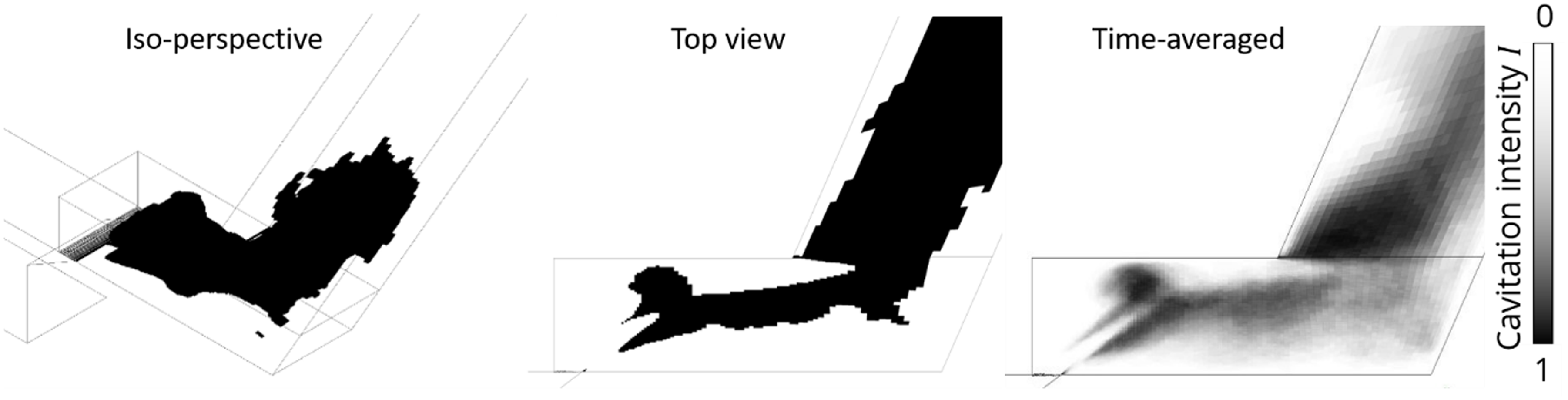
Figure 10. Virtual shadowgraphy; $p_{1}=16.2\,{\rm bar},\ p_{2}=1.2\,{\rm bar}, Q=28\,{\rm l}\,{\rm min}^{-1};\ X=0.92$
.
$p_{1}=16.2\,{\rm bar},\ p_{2}=1.2\,{\rm bar}, Q=28\,{\rm l}\,{\rm min}^{-1};\ X=0.92$
.
5.4 Simulation results and validation with visualisation data
In figure 11a, the simulation results of the CFD model for the spatial distribution of cavitation intensity are compared with the experiment. It is evident that the simulation calculates the spatial cavitation distribution in good agreement with the experiments. However, in the upper left corner of the valve chamber, too little gas fraction is calculated at intense operating points, see last line in figure 11. In contrast to the experiment, the air does not accumulate in the simulation at this point. This is a consequence of the equilibrium modelling, whereby the modelled air fraction immediately decreases again when the pressure rises. The effects of this model error on the erosion calculation are estimated to be low, as the effect is weak and locally limited, and the remaining cavitation distribution, especially in the erosion areas, agrees well with the experiments.
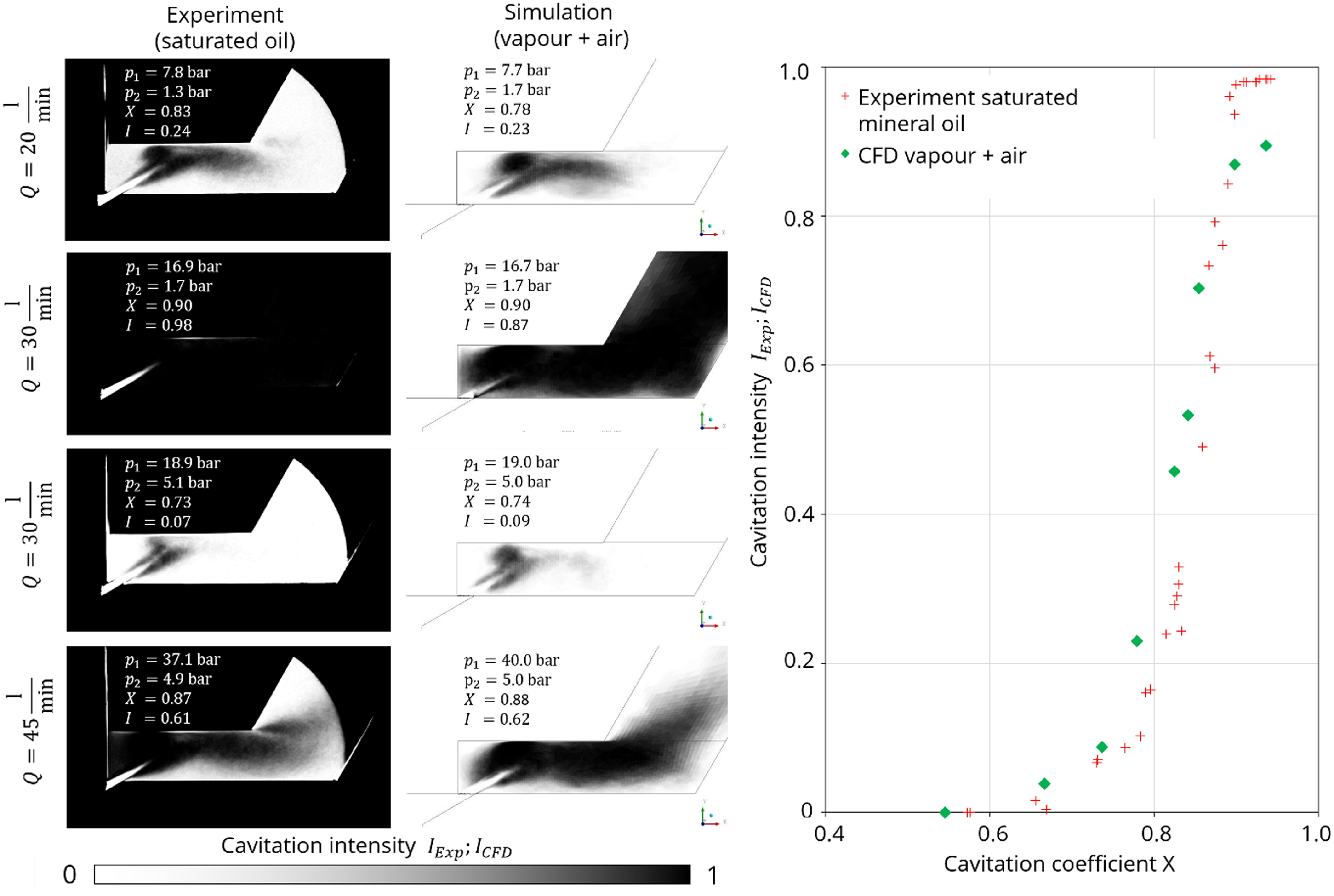
Figure 11. Comparison of the spatial distribution of cavitation intensities between saturated experiments and simulation results.
Comparably good results are observed for the integral cavitation intensity in figure 11b. It can be seen that the beginning and trend of the simulated integral cavitation intensity aligns with the experimental data for most operating points. However, the value of one is not achieved due to the previously discussed non-accumulation of air in the simulation. An important characteristic of the CFD model is that, unlike the Lifante model, the cavitation intensity monotonically increases with the cavitation coefficient. The simulation results are consistent, plausible and no model limitations are observed, thereby enabling the model to be used for erosive operating points.
5.5 Simulative quantification of the location and intensity of the cavitation load
The presented CFD model is used to localise and quantify the location and relative strength of the cavitation load. Additionally, it allows for the numerical investigation of the damping effect of air on the erosion, as observed in the experiment. The inlet and outlet pressures of the erosion test V8 are set as boundary conditions $p_{1}=143\text{ bar}, p_{2}=3.5\text{ bar}$
. To quantify the cavitation load, the four cavitation indices according to Nohmi are implemented and evaluated as field variables in a plane 0.5 mm below the surface, see (13)–(16). After a run-in time of 10 000 time steps, the field variables are averaged over the following 50 000 time steps and evaluated.
$p_{1}=143\text{ bar}, p_{2}=3.5\text{ bar}$
. To quantify the cavitation load, the four cavitation indices according to Nohmi are implemented and evaluated as field variables in a plane 0.5 mm below the surface, see (13)–(16). After a run-in time of 10 000 time steps, the field variables are averaged over the following 50 000 time steps and evaluated.
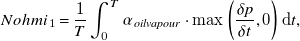 \begin{equation}Nohmi_{1}=\frac{1}{T}\int _{0}^{T}\alpha _{\textit{oilvapour}}\cdot \max \left(\frac{\delta p}{\delta t},0\right)\mathrm{d}t,\end{equation}
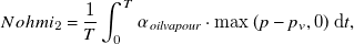 \begin{equation}Nohmi_{2}=\frac{1}{T}\int _{0}^{T}\alpha _{\textit{oilvapour}}\cdot \max \left(p-p_{v},0\right)\mathrm{d}t,\end{equation}
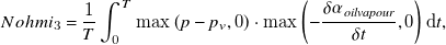 \begin{equation}Nohmi_{3}=\frac{1}{T}\int _{0}^{T}\max \left(p-p_{v},0\right)\cdot \max \left(-\frac{\delta \alpha _{\textit{oilvapour}}}{\delta t},0\right)\mathrm{d}t,\end{equation}
 \begin{equation}Nohmi_{4}=\frac{1}{T}\int _{0}^{T}\max \left(-\frac{\delta \alpha _{\textit{oilvapour}}}{\delta t},0\right)\mathrm{d}t.\end{equation}
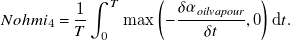
A frequently encountered method in the literature for localising cavitation erosion involves the evaluation of the vapour concentrations. Figure 12 exemplarily compares the volumetric vapour concentration $\alpha _{\textit{oilvapour}}$
with the cavitation index
$\alpha _{\textit{oilvapour}}$
with the cavitation index $Nohmi_{1}$
, revealing the qualitative differences between the two evaluation methods. A simple quantification of cavitation erosion via the vapour concentration falsely predicts the location of the strongest cavitation erosion on the surface of the slopes. No erosion was observed at this point in any experiment. Consequently, the localisation and quantification of cavitation erosion via the vapour concentration is not possible here, as the areas of highest vapour concentration do not agree with the erosion areas. In contrast, the cavitation indices provide the surface where erosion is observed in the experiment. The flow examined here is a good example that cavitation erosion does not necessarily have to occur in the areas with the highest vapour concentration, and underscores the importance of the cavitation erosion indices.
$Nohmi_{1}$
, revealing the qualitative differences between the two evaluation methods. A simple quantification of cavitation erosion via the vapour concentration falsely predicts the location of the strongest cavitation erosion on the surface of the slopes. No erosion was observed at this point in any experiment. Consequently, the localisation and quantification of cavitation erosion via the vapour concentration is not possible here, as the areas of highest vapour concentration do not agree with the erosion areas. In contrast, the cavitation indices provide the surface where erosion is observed in the experiment. The flow examined here is a good example that cavitation erosion does not necessarily have to occur in the areas with the highest vapour concentration, and underscores the importance of the cavitation erosion indices.
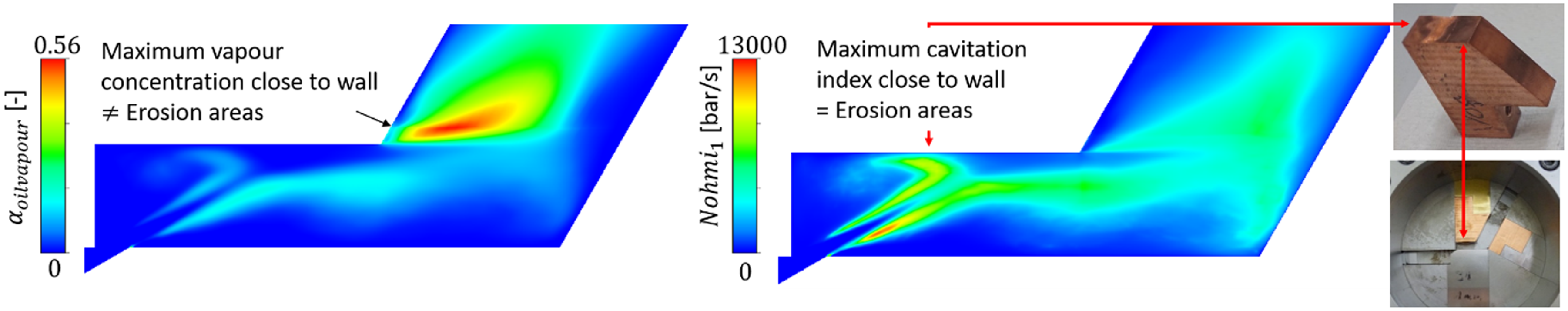
Figure 12. Time-averaged vapour concentration $\alpha _{\textit{oilvapour}}$
and value of the cavitation erosion index
$\alpha _{\textit{oilvapour}}$
and value of the cavitation erosion index $Nohmi_{1}$
in the midplane for air-free oil; photo of the erosion samples.
$Nohmi_{1}$
in the midplane for air-free oil; photo of the erosion samples.
In figure 13 for the air-free case, the time-averaged cavitation indices at a plane 0.5 mm, as recommended by Nohmi et al. (Reference Nohmi, Ikohagi and Iga2008), below the wall are plotted next to the surface scans of the experiment. It can be observed that the cavitation load calculated by indices 1, 3 and 4 aligns very well in location and intensity with the erosion observed in the experiment. Index 2 deviates most significantly from the observations and the other indices. The reason for this lies in the fact that $Nohmi_{2}$
is the only index that does not include the rate of change, see (14). In addition to the general position and shape of the erosion areas, indices 1, 3 and 4 can also predict relevant details such as the very high erosion at the edges, where the pressure peaks to 400 bar.
$Nohmi_{2}$
is the only index that does not include the rate of change, see (14). In addition to the general position and shape of the erosion areas, indices 1, 3 and 4 can also predict relevant details such as the very high erosion at the edges, where the pressure peaks to 400 bar.

This local increase in the cavitation load is caused by the longitudinal vortices that form exactly at these locations. Figure 14 visualises the complex vortex structures within the valve chamber using the $\lambda _{2}$
-criterion. In addition to the cross-vortices, very strong longitudinal vortices form on the front and rear walls, which lead to an additional cavitation load. The longitudinal vortices are induced by the high velocity gradient between the free jet
$\lambda _{2}$
-criterion. In addition to the cross-vortices, very strong longitudinal vortices form on the front and rear walls, which lead to an additional cavitation load. The longitudinal vortices are induced by the high velocity gradient between the free jet $(|u_{\textit{freejet}}| \approx 200\,\mathrm{m}\ \mathrm{s}^{-1}$
) and the wall (no slip condition:
$(|u_{\textit{freejet}}| \approx 200\,\mathrm{m}\ \mathrm{s}^{-1}$
) and the wall (no slip condition: $(|u_{wall}| = 0$
), which causes the vortices to roll up. The longitudinal vortices are thus a consequence of the wall influence and show the strong three-dimensional character of the planar flow geometry. The degree of detail achieved with the CFD model and the Nohmi indices is surprising and impressive.
$(|u_{wall}| = 0$
), which causes the vortices to roll up. The longitudinal vortices are thus a consequence of the wall influence and show the strong three-dimensional character of the planar flow geometry. The degree of detail achieved with the CFD model and the Nohmi indices is surprising and impressive.
Figure 14. Vortex structures in the valve chamber visualised by $\lambda _{2}$
-iso-surfaces; detailed view of the longitudinal vortices with velocity vectors.
$\lambda _{2}$
-iso-surfaces; detailed view of the longitudinal vortices with velocity vectors.
With the cavitation indices according to Nohmi in combination with LES turbulence modelling and validation cavitation model for mineral oil, the cavitation load for this complex three-dimensional free jet flow can be quantified in detail in terms of location and intensity.
5.6 Influence of air on the cavitation load
Figure 15 shows the $Nohmi_{1}$
erosion index for different air mass fractions
$Nohmi_{1}$
erosion index for different air mass fractions $r_{L}$
in the ‘oil–air phase’. It can be observed that the calculated cavitation load decreases with increasing content of air in area size and in the maximum values. To quantify the total cavitation load
$r_{L}$
in the ‘oil–air phase’. It can be observed that the calculated cavitation load decreases with increasing content of air in area size and in the maximum values. To quantify the total cavitation load $\overline{\textit{Nohmi}}_{i}$
, an erosion surface
$\overline{\textit{Nohmi}}_{i}$
, an erosion surface $A_{\textit{Erosion},i}$
is defined using an iso-line e.g.
$A_{\textit{Erosion},i}$
is defined using an iso-line e.g. $Nohmi_{1,4000}$
and the indices are integrated over this area, see (17). The reasoning behind introducing a threshold value is based on the observation that small cavitation loads do not cause erosion damage, aligning with the perspective that cavitation erosion is a fatigue process.
$Nohmi_{1,4000}$
and the indices are integrated over this area, see (17). The reasoning behind introducing a threshold value is based on the observation that small cavitation loads do not cause erosion damage, aligning with the perspective that cavitation erosion is a fatigue process.
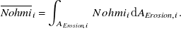 \begin{equation}\overline{\textit{Nohmi}}_{i}=\int _{{A_{\textit{Erosion},i}}}Nohmi_{i}\mathrm{d}A_{\textit{Erosion},i}.\end{equation}
Although the specific selection of the integration region by the threshold value $Nohmi_{i,iso}$
influences the calculated absolute value, it has no influence on the qualitative progression of the curves within reasonable limits. This is illustrated in figure 16 using the example
$Nohmi_{i,iso}$
influences the calculated absolute value, it has no influence on the qualitative progression of the curves within reasonable limits. This is illustrated in figure 16 using the example $\overline{\textit{Nohmi}}_{1}$
by varying the threshold value
$\overline{\textit{Nohmi}}_{1}$
by varying the threshold value $Nohmi_{i,iso}$
by ±50 %. Regardless of the choice of threshold value, the cavitation load decreases with increasing air content.
$Nohmi_{i,iso}$
by ±50 %. Regardless of the choice of threshold value, the cavitation load decreases with increasing air content.
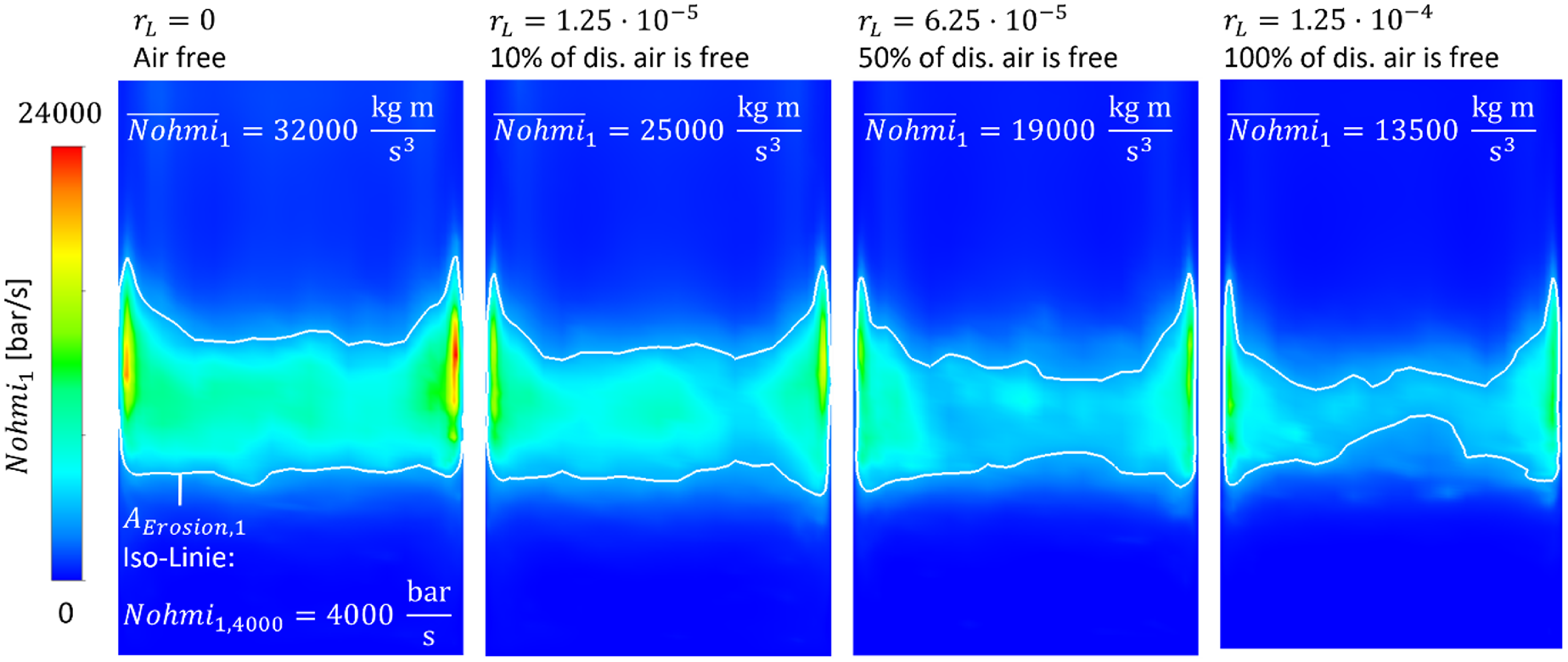
Figure 15. Cavitation index $Nohmi_{1}$
with different air contents.
$Nohmi_{1}$
with different air contents.

Figure 16. Influence of the integration area $A_{\textit{Erosion},1}$
defined by the threshold
$A_{\textit{Erosion},1}$
defined by the threshold $Nohmi_{1,iso}$
on the cavitation load
$Nohmi_{1,iso}$
on the cavitation load $\overline{\textit{Nohmi}}_{1}$
.
$\overline{\textit{Nohmi}}_{1}$
.
For comparability and de-dimensionalisation, the indices are standardised to the respective air-free case,
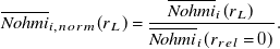 \begin{equation}\overline{\textit{Nohmi}}_{i,norm}(r_{L})=\frac{\overline{\textit{Nohmi}}_{i}(r_{L})}{\overline{\textit{Nohmi}}_{i}(r_{rel}=0)}.\end{equation}
Figure 17
a shows the calculated total cavitation load of the four indices with different mass fractions of free air. The measured air fractions of the air-free experiment is $r_{L,expV8}=0$
and of the saturated experiment
$r_{L,expV8}=0$
and of the saturated experiment $r_{\textit{LexpV}9}=1.5\pm 1\times 10^{-5}$
. It can be seen that even with a low proportion of free air of 10 %–20 % of the maximum soluble air volume, the cavitation load is reduced by approximately 20 % compared with the air-free case. Even this relatively small reduction in the load leads to a disproportionate reduction in cavitation erosion, as the damage usually scales over-proportionally with the load in damage processes. The damping effect of the air observed in the experiment is therefore also reproduced by the CFD model.
$r_{\textit{LexpV}9}=1.5\pm 1\times 10^{-5}$
. It can be seen that even with a low proportion of free air of 10 %–20 % of the maximum soluble air volume, the cavitation load is reduced by approximately 20 % compared with the air-free case. Even this relatively small reduction in the load leads to a disproportionate reduction in cavitation erosion, as the damage usually scales over-proportionally with the load in damage processes. The damping effect of the air observed in the experiment is therefore also reproduced by the CFD model.
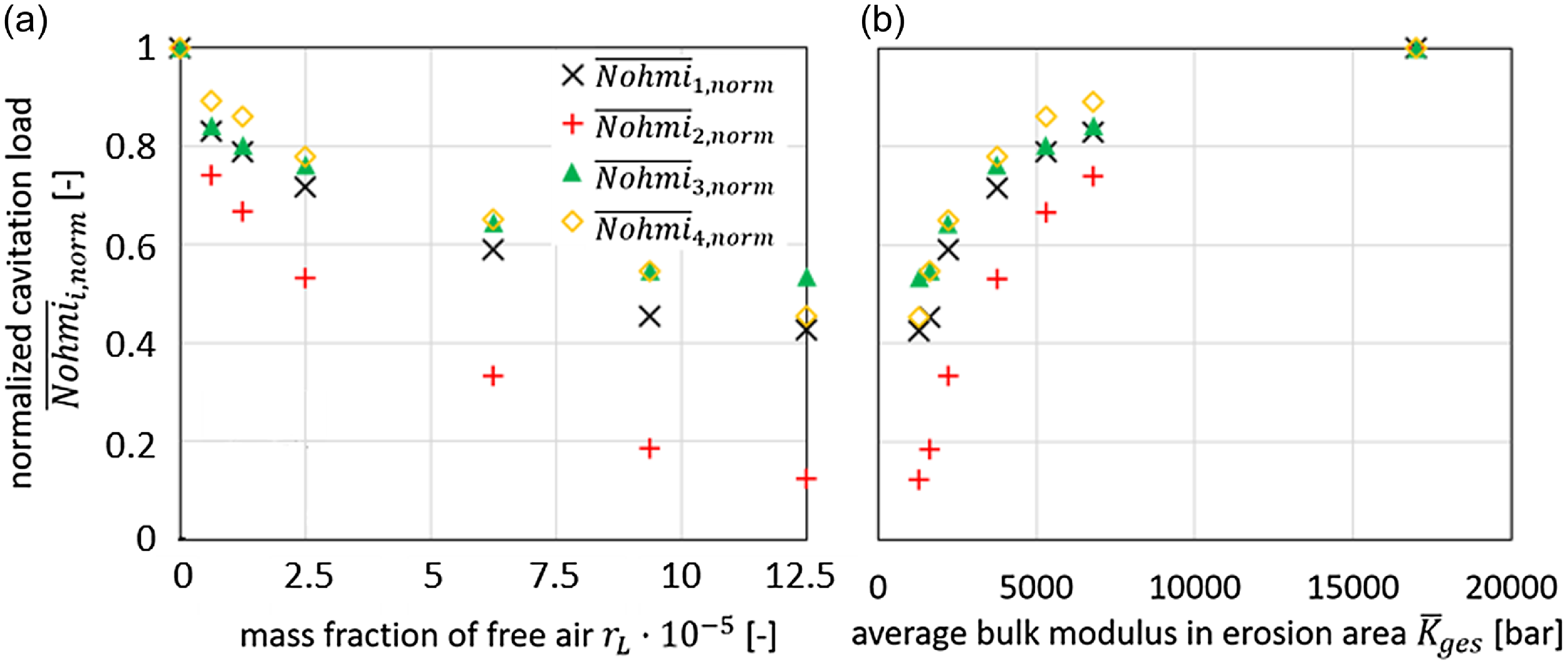
Figure 17. (a) Influence of the air on the simulated cavitation load. (b) Influence of the compression modulus averaged over $A_{\textit{Erosion},i}$
on the normalised cavitation load.
$A_{\textit{Erosion},i}$
on the normalised cavitation load.
The cause of the reduction in erosion load with increasing air content can be seen in figure 17b, in which the total erosion is plotted against the area-averaged compression modulus of the ‘oil–air phase’ $\overline{K}_{ges}$
,
$\overline{K}_{ges}$
,
 \begin{equation}\overline{K}_{ges}=\frac{1}{A_{\textit{erosion}}}\int _{{A_{\textit{Erosion}}}}K_{ges} \mathrm{d}A.\end{equation}
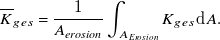
The lower the compression modulus, the less total erosion is calculated. This simulation result supports the hypothesis that the erosion-damping effect of air is caused by a reduction in fluid stiffness. This is physically plausible, as locally excited pressure changes in a compliant fluid have lower maximum values and smaller rates of change than in a stiffer fluid. A soft fluid reduces pressure surges and pressure change rates, and therefore has a positive effect on cavitation loads. Additionally, weakened pressure minima lead to reduced vapour productions, because bubble creation is driven by local and momentary pressure. Both lower pressure change rates $\dot{p}_{rms}$
and lower vapour volume fractions
$\dot{p}_{rms}$
and lower vapour volume fractions $\alpha _{\textit{oilvapour}}$
are observed in simulations with higher air mass fractions
$\alpha _{\textit{oilvapour}}$
are observed in simulations with higher air mass fractions $r_{L}$
, see figure 18.
$r_{L}$
, see figure 18.
Figure 18. Time-averaged vapour volume fraction and pressure change rates for different air fractions.
6. Summary and outlook
Cavitation erosion leads to several damages which limit the lifetime and operational range of hydraulic components and systems. By means of CFD, it seems possible to optimise the flow to reduce or relocate erosion areas. However, the correct simulative localisation of cavitation erosion in oil-hydraulic components has proven difficult in the past. The main reasons are seen in: lack of separation between vapour and gas cavitation; uncertain parametrisation of cavitation models; controversial influence of free air on cavitation erosion; weak turbulence modelling with RANS; neglecting of the stochastic nature of cavitation and locating the erosion areas via the vapour volume fraction.
On the experimental side, a test rig is presented in which the air content can be freely adjusted and measured. Hence, it is possible to separated gas and vapour cavitation by completely degassing the fluid. The flow geometry is a transparent spool valve with optical access and removable erosions probe. The cavitating flow is visualised using a high-speed camera and the statistical shadowgraphy method for many different conditions and saturations. In addition, erosion tests are performed with different air contents, which experimentally proved that cavitation erosion is caused by vapour cavitation – not gas cavitation. In fact, the air released by gas cavitation dampens the cavitation erosion by a factor of 4–5, see figure 2.
On the simulation side, the visualisation data were used to parametrise and validate Euler–Euler cavitation models. In particular, the Zwart–Gerber–Belamri model with optimised empirical parameters for mineral oil showed excellent results for the damage-relevant vapour cavitation. To take the influence of air into account, an additional ‘oil–air’ phase is introduced. All phases are modelled as compressible to reflect pseudo-cavitation.
The simulation results of the spatial cavitation distribution are compared with the visualisation data, which show good agreement, see figures 4 and 11. It was shown that turbulence modelling with LES is essential, since it resolves vortices, and the local and momentary pressure field and thus the cavitation correctly.
The model is then used to relatively quantify the cavitation erosion load under intense conditions. It is shown that the areas of maximum vapour concentration near the wall are not congruent with the observed erosion regions. Hence, it is not a suitable indicator. In contrast to this, the cavitation indices by Nohmi succeed well in reflecting the location, shape and intensity of cavitation erosion, see figure 13. Even local details such as the increased mass loss at the edges are reflected with high precision. The simulation now allows the cause of these local effects to be analysed, which lies in the formation of strong longitudinal vortices precisely at these points, see figure 14.
The model also reflects the experimentally observed damping effect of air, see figure 15. The simulation results support the hypothesis that the erosion-damping effect of air is caused by the reduction in fluid stiffness, as pressure minima and the dynamics of bubble collapses are weakened, see figures 16 and 17.
The key factors for a successful CFD simulation of cavitation erosion in hydraulic components are:
-
• high temporal and spatial resolution of the pressure field and its fluctuations, in particular, resolution of local vortex structures using LES turbulence modelling – not RANS;
-
• clear separation of cause and effect of vapour and gas cavitation;
-
• detailed parametrisation and validation of the cavitation model, in particular, the damage-relevant vapour cavitation by means of flow visualisation, e.g. shadowgraphy;
-
• quantification of the cavitation load by means of cavitation indices, not vapour volume fraction;
-
• statistical analysis – not momentary states.
It seems highly interesting to apply the methodology presented to other flows. For hydraulic valves and pumps in particular, the probability of success is considered to be high, as these are fluid mechanically similar free jet flows. This assumption is supported by the fact that the geometry investigated is already a realistic valve flow with complex, three-dimensional details, such as the locally excessive mass loss on the edges due to vortices.
Based on the positive results of the experiments and simulations, the use of the presented cavitation model and the cavitation erosion indices for the further development of pumps and valves in industrial practice is consistent and promising from the author’s point of view. Their use in the development process enables the early identification and analysis of cavitation-related problems and the virtual testing of potential countermeasures. This allows the development process to be accelerated, the service life to be increased and the operating range to be extended to higher power densities of hydraulic components.
The CFD technique presented is ready for use and the authors encourage anyone who simulates cavitation in hydraulic valves and pumps to test the presented model and provide feedback.
Many more details on the subject of cavitation in oil hydraulic components with regards to visualisation, simulation and erosion can be found in the author’s dissertation (Osterland, Reference Osterland2024).
Acknowledgements
The authors gratefully acknowledge the GWK support by providing computing time through the Center for Information Services and HPC at TU Dresden.
Funding
The presented research activities are part of the projects ‘Parametrierung von Kavitationsmodellen für die gezielte Betriebsbereichserweiterung ölhydraulischer Komponenten und Systeme’ and ‘Kavitationserosion verschiedener Druckflüssigkeiten und deren Mischungskomponenten’. The authors would like to thank the Fluid Power Research Fund of the VDMA for the funding and support.
Competing interests
The authors declare no conflict of interest.
Author biographies
Dr.-Ing. Sven Osterland received his diploma in Diploma in Mechanical Engineering in the fields of structural durability from TU Dresden in 2014. Since 2015, he has been working as a Research Associate at the Chair of Fluid-Mechatronic Systems (Fluidtronics), Institute of Mechatronic Engineering, Technische Universität Dresden and finished his doctorate in 2024. His research areas include numerical multiphase flow simulations (CFD), experimental flow visualisation of cavitating flows and cavitation erosion in hydraulic components.
Prof. Jürgen Weber was appointed on 1st March 2010 as a University Professor and the Chair of Fluid-Mechatronic Systems as well as the Director of the Institute of Fluid Power at the Technische Universität Dresden, and took on the leadership of the Institute of Mechatronic Engineering in 2018. He finished his doctorate in 1991 and was an active Senior Engineer at the former Chair of Hydraulics and Pneumatics until 1997. This was followed by a 13-year industrial phase. In addition to his role as the Head of the Department Hydraulics and Design Manager for Mobile and Tracked Excavators, starting in 2002, he took on responsibility for the hydraulics in construction machinery at CNH Worldwide. From 2006 onwards, he was the Global Head of Architecture for hydraulic drive and control systems, system integration and advance development CNH construction machinery.

Appendix A: Visualisation data (Osterland, Reference Osterland2024)
Table A1. Overview of the operation points and results of the 99 visualisation experiments

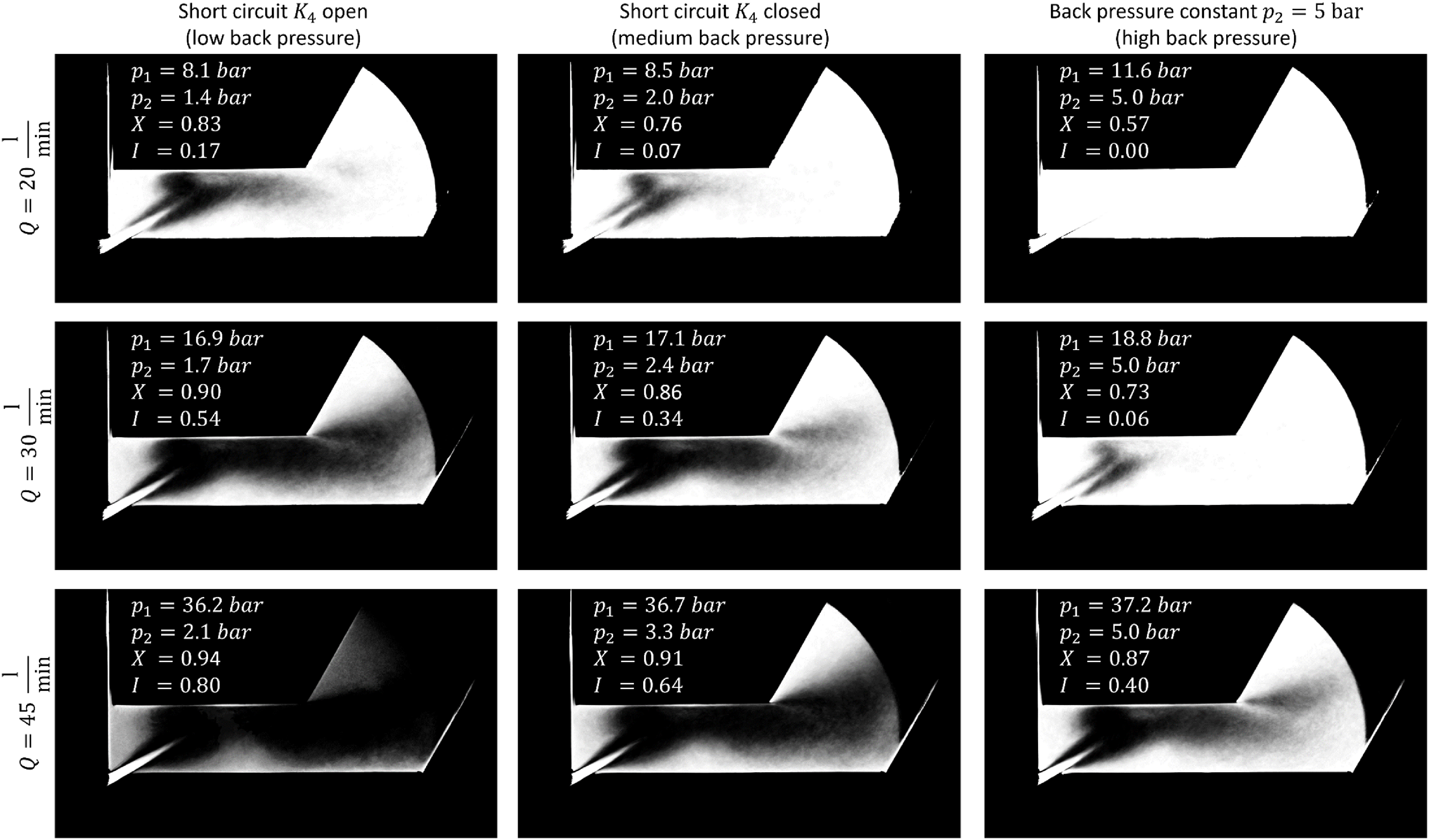
Figure A1. Time-averaged cavitation intensity of air-free mineral oil at different volume flows and back pressures.

Figure A2. Time-averaged cavitation intensity of saturated mineral oil at different volume flows and back pressures.
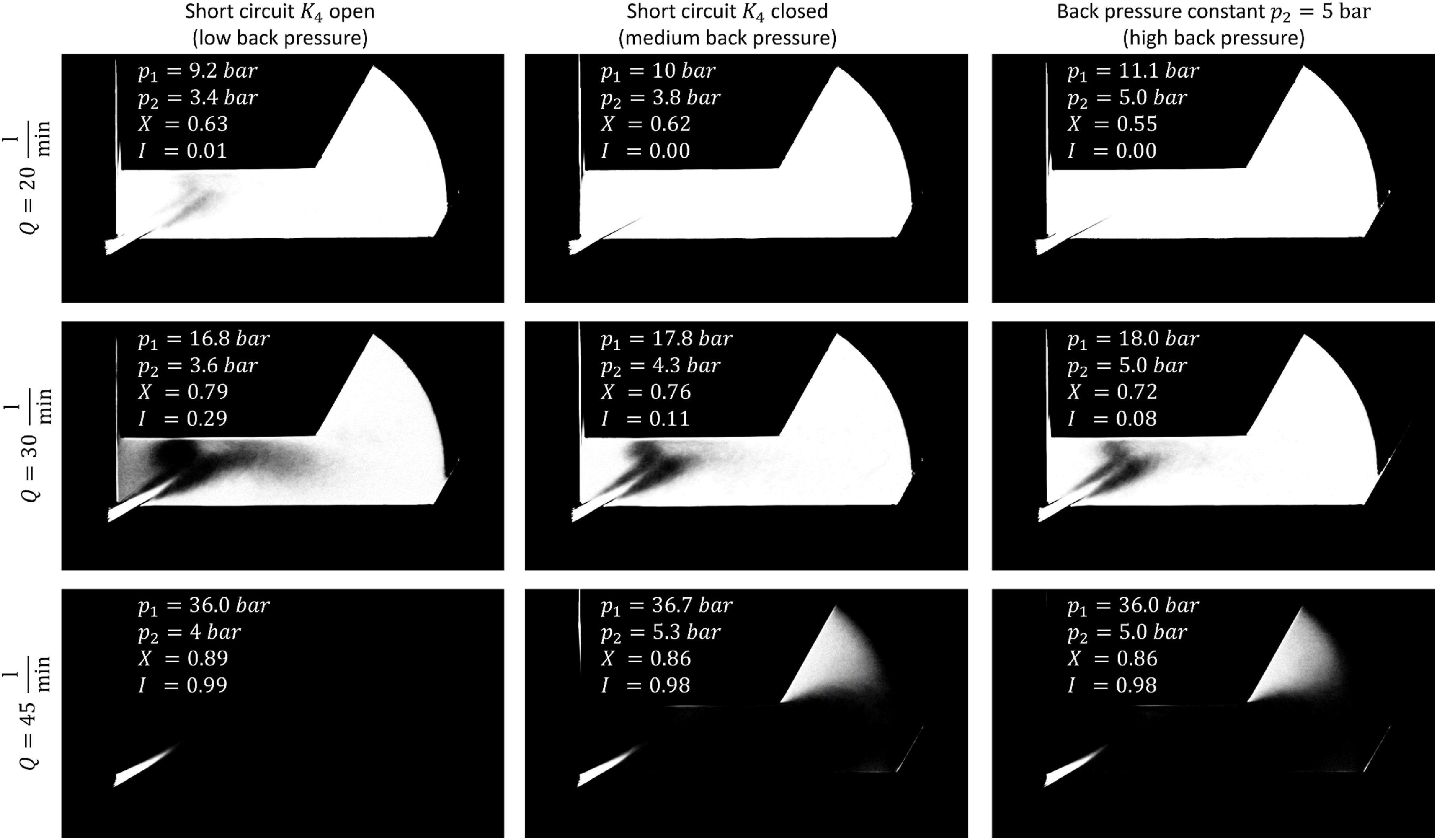
Figure A3. Time-averaged cavitation intensity of 3 times oversaturated mineral oil at different volume flows and back pressures.


 Open access