


Impact Statement
Gravity-driven thin flows are common occurrences in everyday life as witnessed, for example, when rainwater drains along a sloped pavement. Here, we present a comparative study of depth-integrated models that describe three-dimensional thin flows over topography. Three models are discussed in detail with a focus on their mathematical formulation, as well as on a practical numerical solution procedure using finite differences. Various fully submerged topographies are selected to illustrate the versatility of the models. These include a smooth Gaussian bump, a rectangular steep-sided trench and a wavy bottom. Because these flows are prone to interfacial instabilities along the free surface, the stability of the flow for a flat inclined bottom is also discussed in detail. Students and researchers new to this topic will benefit from the friendly introduction to the background and fundamental concepts, while those already familiar with this subject will also gain some insight into useful methods and techniques to better understand these interesting flows.
1. Introduction
Falling thin viscous flows are ubiquitous in both natural and human-made settings (Reference Alekseenko, Nakoryakov and PokusaevAlekseenko, Nakoryakov & Pokusaev 1994; Reference ChangChang 1994; Reference Chang and DemekhinChang & Demekhin 2002; Reference Craster and MatarCraster & Matar 2009; Reference Kalliadasis, Ruyer-Quil, Scheid and VelardeKalliadasis et al. 2012). In industrial applications such layers provide a protective coat on surfaces as in bearings, paintings and other manufacturing processes (Reference Kistler and SchweizerKistler & Schweizer 1997). On the other hand, in the environment thin flows can be found in rivers, or may appear as lava flows (Reference Huppert, Shepherd, Sigurdsson and SparksHuppert et al. 1982; Reference GriffithsGriffiths 2000), ice flows (Reference Rignot, Mouginot and ScheuchlRignot, Mouginot & Scheuchl 2011), mud slides (Reference Ng and MeiNg & Mei 1994) or even avalanches (Reference Hákonardóttir, Hogg, Batey and WoodsHákonardóttir et al. 2003). Whereas in living organisms, thin fluid layers are known to play a vital role in lining the airways in lungs, and in the case of a tear film they form a protective surface on the front of the eye (Reference BraunBraun 2012). Other examples include thin flows in human-made structures such as aqueducts and spillways. Because thin fluid layers are susceptible to interfacial instabilities, variations in fluid thickness typically occur, and this can lead to the formation of waves propagating along the surface which can have adverse effects. In coating applications, for example, this can produce uneven coatings. In human-made conduits such as open aqueducts, spillways of dams and runoff channels, the flow instability generates a series of intermittent bores, known as roll waves, with surges that can damage flow control and flow measuring devices, and can even raise the fluid level above the channel walls. In naturally occurring debris flows, surface bores can drastically increase their destructive power. As a result of this, thin fluid layers have been studied extensively. The first experiments were conducted by the father and son Reference Kapitza and KapitzaKapitza & Kapitza (1949), while the first theoretical predictions for the onset of instability were made by Reference BenjaminBenjamin (1957), then Reference YihYih (1963) and later by Reference BenneyBenney (1966). Reference ShkadovShkadov (1967) was the first to construct a simplified mathematical model for these flows. In the literature one can find a plethora of two-dimensional investigations, but relatively few three-dimensional studies. Before proceeding further, it is worth defining what we mean by two- and three-dimensional flows. Depending on the number of independent variables used, bottom topographies are either one- or two-dimensional. The flow over a one-dimensional topography is defined to be two-dimensional (ignoring three-dimensional patterns arising from instabilities), while the flow over a two-dimensional topography is defined to be three-dimensional. This definition is consistent with that adopted by Reference Aksel and SchörnerAksel & Schörner (2018) and others.
Owing to the numerous applications cited above, considerable effort has been invested in modelling two-dimensional isothermal thin fluid layers. When the governing Navier–Stokes equations are cast in dimensionless form, two dimensionless parameters emerge: the Reynolds number ( $Re$) and the Weber number ( $We$). If the streamwise length scale is different from the cross-stream length scale, then another dimensionless parameter given by the ratio of these length scales appears. This is known as the shallowness parameter, $\delta$, and for thin fluid layers $\delta \ll 1$. The key finding discovered by Reference BenjaminBenjamin (1957), Reference YihYih (1963) and Reference BenneyBenney (1966) is that the critical Reynolds number, beyond which thin flow down a flat surface inclined at an angle of $\beta$ with the horizontal becomes unstable, is given by $Re_{crit} = 5 \cot \beta /6$. For the applications listed above the Reynolds number can range from small to moderate values, and hence the flows can vary from a stable flow having a uniform thickness to an unstable flow with waves propagating along the free surface. For the cases presented in this study, we focus on Reynolds numbers of order unity near criticality.
As noted above, the two-dimensional flow over a flat bottom becomes unstable when  $Re_{crit} = 5 \cot \beta /6$. The influence of wavy bottom topography on the stability of a flow has been discussed in several previous studies. For example, Reference D'Alessio, Pascal and JasmineD'Alessio, Pascal & Jasmine (2009) using the weighted-residual (WR) model showed that with weak to moderate surface tension bottom topography acts to stabilize the flow, while with strong surface tension bottom topography can destabilize the flow provided the wavelength of the bottom undulation is sufficiently short. The stabilizing effect of bottom topography on inclined flows was also reported by Reference Wierschem, Lepski and AkselWierschem, Lepski & Aksel (2005) for weak surface tension, whereas the reversal in the stabilizing action of bottom topography was noted by Reference Heining and AkselHeining & Aksel (2009) and Reference Häcker and UeckerHäcker & Uecker (2009) using the WR model. Reference Heining and AkselHeining & Aksel (2009) discovered this by investigating the inverse problem, that is, they sought the corresponding bottom topography that gave rise to a free-surface profile. On the other hand, Reference Häcker and UeckerHäcker & Uecker (2009) addressed the direct problem by expressing the equations of motion in terms of curvilinear coordinates relative to the bottom profile. The work by Reference Heining and AkselHeining & Aksel (2010) demonstrated that the critical Reynolds number of the neutral stability curve shifts for gravity-driven films over corrugated bottoms compared with that over flat bottoms. Moreover, the shift depends on several parameters. For large bottom corrugations the study conducted by Reference Wierschem and AkselWierschem & Aksel (2003) showed that the fluid particles do not follow the complete solid bottom contour; instead, the particles slide on the separatrix of eddies created in the valleys of the bottom corrugations. In these cases the neutral stability curve changes drastically. For such complex flow structures integral boundary layer (IBL) or WR simulations are not available in the literature.
In this investigation we are primarily interested in the hydrodynamic mode of instability, known as the H mode, which is the result of long-wave deformations of the free surface due to inertia. It occurs in both isothermal and non-isothermal flows. The stability of the H mode was originally studied theoretically by Reference BenjaminBenjamin (1957), Reference YihYih (1963) and Reference BenneyBenney (1966), while experiments were first carried out by Reference Kapitza and KapitzaKapitza & Kapitza (1949), and later by Reference Liu, Paul and GollubLiu, Paul & Gollub (1993). The physical mechanism for this long-wave instability was advanced by Reference SmithSmith (1990). The scaling adopted in § 2 is well suited to analyse the H mode. Although there is a shear mode, it has been shown by Reference Floryan, Davis and KellyFloryan, Davis & Kelly (1987) that this mode will only be important at small inclination angles. In addition, there are also P and S modes of instability that arise when a thin film flows over a heated substrate. These modes were identified by Reference Goussis and KellyGoussis & Kelly (1991), and were also investigated by Reference PearsonPearson (1958) and Reference SmithSmith (1966). In fact, Reference SmithSmith (1966) suggested that the instability observed by Reference BénardBénard (1900) was likely due to the Marangoni effect rather than to buoyancy effects. In order to capture the P and S modes one needs to introduce a second scaling because the parameters involved in the neutral stability relation are in fact implicitly dependent on the Reynolds number. Thus, a rescaling of the problem must be considered which involves strictly independent parameters in order to ensure that all physical aspects are fully and correctly taken into account.
To accurately represent an unsteady and non-uniform flow arising from interfacial instability, a mathematical model must incorporate all the relevant physical factors, and possess the mathematical complexity required to capture the spatiotemporal coupling and nonlinear dynamics of the flow. At the same time, simplifications to the governing equations, warranted by physically justified assumptions, can lead to a more complete and productive mathematical treatment. A general modelling approach is to reduce the space dimensionality of the problem, and to exploit the assumed shallowness of the flow which enables depth integration of the equations of motion. This strategy requires that the velocity variation with depth is consistent with laminar flow, and hence can be specified a priori. A suitable approximation can be constructed from the self-similar parabolic velocity profile resulting from a balance between gravity and longitudinal shear which governs the steady uniform flow. Applying boundary conditions at the top and bottom of the fluid layer then introduces the dependence on the fluid thickness which will be transient and non-uniform for unstable flows. This leads to a two-equation system for the thickness and flow rate of the fluid layer which is referred to as the IBL model. This was first developed by Reference ShkadovShkadov (1967) for two-dimensional flows. Although the IBL model can successfully reproduce certain aspects of the flow, it overpredicts the critical conditions for the onset of instability for two-dimensional flow over a flat bottom, when compared with the results from the Orr–Sommerfeld equations (Reference BenjaminBenjamin 1957; Reference YihYih 1963) and the experimental work of Reference Liu, Paul and GollubLiu et al. (1993). Despite efforts to rectify the IBL model (Reference Prokopiou, Cheng and ChangProkopiou, Cheng & Chang 1991; Reference UeckerUecker 2003), erroneous overpredictions for the onset of instability plagued all attempts.
An alternative approach was proposed by Reference Ruyer-Quil and MannevilleRuyer-Quil & Manneville (2000, Reference Ruyer-Quil and Manneville2002) where they considered a more accurate velocity profile obtained by means of a weighted-residual technique having a polynomial expansion for the velocity. Their model, known as a WR model, also consists of a two-equation system in terms of the flow rate and fluid thickness. More importantly, the WR model is able not only to correctly predict the critical conditions for the onset of instability, but also to capture the development of the supercritical flow as revealed by comparisons with the laboratory experiments of Reference Liu, Schneider and GollubLiu, Schneider & Gollub (1995) and the direct numerical simulations of Reference Ramaswamy, Chippada and JooRamaswamy, Chippada & Joo (1996). The ability of this model to accurately describe flows under unstable conditions far from criticality qualifies it as an important improvement over the Benney equation (Reference BenneyBenney 1966) which is only valid near the instability threshold.
The success of the WR model created a lot of interest in extending it to more complex flows. For example, Reference Kalliadasis, Demekhin, Ruyer-Quil and VelardeKalliadasis et al. (2003) applied the WR formulation to model flows down an even heated incline, Reference D'Alessio, Pascal and JasmineD'Alessio et al. (2009) used it to model isothermal flows over a wavy incline, while Reference Pascal and D'AlessioPascal & D'Alessio (2010) successfully applied it to inclined isothermal flows down an uneven porous surface. Several other extensions such as incorporating surfactants (Reference D'Alessio, Pascal, Ellaban and Ruyer-QuilD'Alessio et al. 2020) and heated flows over wavy surfaces (Reference D'Alessio, Pascal, Jasmine and OgdenD'Alessio et al. 2010; Reference Daly, Gaskell and VeremieievDaly, Gaskell & Veremieiev 2022) have also been implemented, to list a few. While most of these WR models listed above are second order in the shallowness parameter, Reference Veremieiev and WacksVeremieiev & Wacks (2019) have extended the WR formalism to include third- and fourth-order terms.
Other approaches used to model slow viscous motion of a thin fluid layer include the application of lubrication theory, or using Stokes flow. Many such investigations are summarized in the thorough review carried out by Reference Aksel and SchörnerAksel & Schörner (2018). Lubrication theory is based on flows possessing a slowly varying cross-section, such as in a journal bearing. If the fluid layer has a thickness,  $H$, which is small compared with its length, $L$, then it can be shown (Reference BatchelorBatchelor 1965; Reference LealLeal 1992) that the left-hand side of the Navier–Stokes equations becomes negligible if $\delta Re \ll 1$, where $\delta = H/L$ is the shallowness parameter mentioned earlier, and to leading order the pressure becomes hydrostatic. Then, retaining terms up to first order in $\delta$ yields parabolic profiles for the horizontal velocities. Finally, integrating the continuity equation across the fluid layer leads to a single nonlinear evolution equation for the fluid thickness. Some early studies include the case of thin-film flow over a one-dimensional trench (Reference Kalliadasis, Bielarz and HomsyKalliadasis, Bielarz & Homsy 2000; Reference Mazouchi and HomsyMazouchi & Homsy 2001; Reference Bielarz and KalliadasisBielarz & Kalliadasis 2003), while Reference Gaskell, Jimack, Sellier, Thompson and WilsonGaskell et al. (2004) considered both one- and two-dimensional topographies. More recently Reference Hinton, Hogg and HuppertHinton, Hogg & Huppert (2019, Reference Hinton, Hogg and Huppert2020a, Reference Hinton, Hogg and Huppert2020b) used lubrication models, asymptotic analyses and laboratory experiments to describe free-surface viscous flows over two-dimensional mounds, around a corner and past cylinders of various cross-sections. Reference D'AlessioD'Alessio (2023a) also used a lubrication model to compute flows past cylinders having circular and elliptical cross-sections.
Turbulent and laminar two-dimensional models based on the shallow-water equations have also been used by Reference Balmforth and MandreBalmforth & Mandre (2004). However, the equations are not methodically derived and rely on empirical terms. For example, the turbulent model included empirical terms to account for turbulent friction and internal dissipation. As pointed out by Reference Prokopiou, Cheng and ChangProkopiou et al. (1991), both periodic and solitary wave solutions to the shallow-water equations modified with a dissipative term produce amplitudes that are strongly dependent on the viscosity coefficient which makes it difficult to estimate the value of this parameter.
Three-dimensional thin fluid layers are intrinsically more complex than their two-dimensional counterparts. Thus, it comes as no surprise that the work devoted to modelling three-dimensional thin fluid layers is relatively rare compared with two-dimensional fluid layers. Listed here are some previous studies pertaining to three-dimensional flows spreading over topography. Reference Baxter, Power, Cliffe and HibberdBaxter et al. (2009) considered steady gravity-driven Stokes flow down an incline and over hemispherical obstacles. Stokes flow corresponds to small-Reynolds-number flows whereby the inertial forces are neglected which leads to a linear balance between viscous and pressure forces. The controlling parameters in their investigation were the angle of inclination, the Bond number and the obstacle geometry. A key finding is that the free-surface profiles had a peak upstream of the obstacle followed by a downstream trough. They also considered cases where the obstacle penetrates the free surface, and in such cases a contact angle was specified. The study by Reference Buttle, Pethiyagoda, Moroney and McCueButtle et al. (2018), on the other hand, considered the steady flow of an ideal fluid using a boundary-integral method. Both subcritical and supercritical regimes were explored for a variety of bottom configurations. Their focus was on the nonlinear features of the wave patterns and their relationship to ship wakes. Reference Veremieiev, Thompson, Lee and GaskellVeremieiev et al. (2010) and Reference Veremieiev, Thompson and GaskellVeremieiev, Thompson & Gaskell (2015) numerically investigated two- and three-dimensional flow over step-like and trench topographies and obtained good agreement with the experimental results of Reference Decré and BaretDecré & Baret (2003). Three-dimensional flows over a wavy bottom were studied theoretically by Reference TrifonovTrifonov (2004); he derived a thin-film IBL model. Reference Heining, Pollak and AkselHeining, Pollak & Aksel (2012) also worked on three-dimensional flows over a wavy bottom and solved the problem analytically, numerically and experimentally. In addition, Reference Hinton, Hogg and HuppertHinton et al. (2019) investigated the flow of a viscous free surface over bottom topography theoretically and numerically through the lens of lubrication theory. Their work was motivated by the interaction of lava flows with obstructions. They considered cases where the topography penetrated the free surface, which they termed dry zones, and where dry zones would form in the wake of an obstacle. Rather than specifying a contact angle, they handled dry zones by introducing a small source term which had the effect of creating a virtual thin film over the dry zone. More recently, Reference D'AlessioD'Alessio (2023b) developed a hybrid model which blends IBL formalism with lubrication theory. Various bottom topographies were considered and good agreement was found with the experimental work of Reference Heining, Pollak and AkselHeining et al. (2012) and with the numerical simulations of Reference Hinton, Hogg and HuppertHinton et al. (2019).
The goal of the present study is to present and contrast three-dimensional IBL, WR and hybrid models. The IBL and WR models were chosen since they tend to be the most common. The hybrid model was also included because it is a cross between the IBL and lubrication models, and as such it can represent lubrication-type models. Numerous numerical experiments are conducted spanning steady subcritical, and unsteady supercritical flows. Various three-dimensional, fully submerged topographical flows are entertained including a smooth localized bump, wavy periodic undulations and a steep-sided trench. The paper is structured as follows. In the next section we formulate the problem mathematically, and derive second-order IBL and WR models for three-dimensional flow. These models are second order in terms of the shallowness parameter,  $\delta$, which is assumed to be small. Following that, in § 3 linear stability analyses are carried out using the three models for the case of a flat inclined bottom to demonstrate that the three-dimensional predictions made for the threshold of instability are in full agreement with those arising from two-dimensional flows. Then in § 4 a new numerical solution procedure is proposed to solve the model equations. Various steady and unsteady results are presented and discussed in § 5; the three models are contrasted and validated by drawing comparisons with experimental data pertaining to a case characterized by a two-dimensional wavy bottom topography. Finally, in § 6 we summarize the main findings. Lastly, Appendix A, which outlines the derivation of the dynamic conditions applied along the free surface, is also included.
2. Mathematical formulation
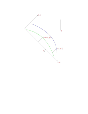
We consider the three-dimensional, laminar, gravity-driven, isothermal flow of a viscous, incompressible, Newtonian, shallow liquid layer of thickness  $h(x,y,t)$ down a non-porous surface which is inclined at an angle of $\beta$ with the horizontal. The surface over which the fluid is flowing has a variable bottom topography denoted by $\mathcal {M}m(x,y)$. Here, $\mathcal {M}$ refers to the amplitude of the bottom topography. We define a coordinate system $(x,y,z)$ such that the down-slope coordinate is $x$, the cross-slope coordinate is $y$ and the normal coordinate above the inclined surface is $z$. Illustrated in figure 1 is a cross-sectional view in the $x$ direction along the centreline.
Cross-section of the flow and set-up.

The continuity and Navier–Stokes equations expressed in dimensional form are given by
 \begin{equation} \left.\begin{gathered}
\frac{\partial u}{\partial x} + \frac{\partial v}{\partial
y} + \frac{\partial w}{\partial z} = 0,\\ \rho
\left(\frac{\partial u}{\partial t} + u \frac{\partial
u}{\partial x} + v \frac{\partial u}{\partial y} + w
\frac{\partial u}{\partial z} \right) = {-} \frac{\partial
p}{\partial x} + \rho g\sin \beta + \mu
\left(\frac{\partial^2 u}{\partial x^2} + \frac{\partial^2
u}{\partial y^2} + \frac{\partial^2 u}{\partial
z^2}\right),\\ \rho \left(\frac{\partial v}{\partial t} + u
\frac{\partial v}{\partial x} + v \frac{\partial
v}{\partial y} + w \frac{\partial v}{\partial z}\right) =
{-} \frac{\partial p}{\partial y} + \mu
\left(\frac{\partial^2 v}{\partial x^2} + \frac{\partial^2
v}{\partial y^2} + \frac{\partial^2 v}{\partial
z^2}\right),\\ \rho \left(\frac{\partial w}{\partial t} + u
\frac{\partial w}{\partial x} + v \frac{\partial
w}{\partial y} + w \frac{\partial w}{\partial z} \right) =
{-} \frac{\partial p}{\partial z} - \rho g\cos \beta + \mu
\left(\frac{\partial^2 w}{\partial x^2} + \frac{\partial^2
w}{\partial y^2} + \frac{\partial^2 w}{\partial
z^2}\right), \end{gathered}\right\}
\end{equation}
\begin{equation} \left.\begin{gathered}
\frac{\partial u}{\partial x} + \frac{\partial v}{\partial
y} + \frac{\partial w}{\partial z} = 0,\\ \rho
\left(\frac{\partial u}{\partial t} + u \frac{\partial
u}{\partial x} + v \frac{\partial u}{\partial y} + w
\frac{\partial u}{\partial z} \right) = {-} \frac{\partial
p}{\partial x} + \rho g\sin \beta + \mu
\left(\frac{\partial^2 u}{\partial x^2} + \frac{\partial^2
u}{\partial y^2} + \frac{\partial^2 u}{\partial
z^2}\right),\\ \rho \left(\frac{\partial v}{\partial t} + u
\frac{\partial v}{\partial x} + v \frac{\partial
v}{\partial y} + w \frac{\partial v}{\partial z}\right) =
{-} \frac{\partial p}{\partial y} + \mu
\left(\frac{\partial^2 v}{\partial x^2} + \frac{\partial^2
v}{\partial y^2} + \frac{\partial^2 v}{\partial
z^2}\right),\\ \rho \left(\frac{\partial w}{\partial t} + u
\frac{\partial w}{\partial x} + v \frac{\partial
w}{\partial y} + w \frac{\partial w}{\partial z} \right) =
{-} \frac{\partial p}{\partial z} - \rho g\cos \beta + \mu
\left(\frac{\partial^2 w}{\partial x^2} + \frac{\partial^2
w}{\partial y^2} + \frac{\partial^2 w}{\partial
z^2}\right), \end{gathered}\right\}
\end{equation}
where  $u,v,w$ are the velocity components in the $x,y,z$ directions, respectively, $p$ is the pressure, $g$ is the acceleration due to gravity, $\rho$ is the density and $\mu$ is the dynamic viscosity. We next cast the governing equations in dimensionless form. In order to achieve this we choose the Nusselt thickness (Reference NusseltNusselt 1916) of the liquid, given by
 \begin{equation} H = \left(\frac{3\mu Q}{g\rho \sin\beta}\right)^{1/3}, \end{equation}
as the vertical length scale, while  $L$ to be the horizontal length scale. For a wavy topography $L$ is typically taken to be the wavelength of the bottom undulations, while for a localized topography such as a bump or trench, $L$ can be taken to be the length or width of the bump or trench. In the above $Q$ denotes the prescribed flow rate per unit width. The velocity scale is taken to be $U = Q/H$ and the time scale is $L/U$. For the pressure we use $\rho U^2$ as the scale. Using these scales we apply the following transformation:
 \begin{equation} \left.\begin{gathered} (x,y,z) = (Lx^{{\ast}},Ly^{{\ast}},Hz^{{\ast}}),\quad h = H h{^\ast},\quad \mathcal{M} = H \mathcal{M}^{{\ast}},\quad t = \frac{L}{U} t^{{\ast}},\\ (u,v,w) = U\left(u^{{\ast}},v^{{\ast}},\frac{H}{L}w^{{\ast}}\right),\quad p = \rho U^2 p^{{\ast}}, \end{gathered}\right\} \end{equation}
where the asterisk denotes a dimensionless quantity. With these scalings in place, and dropping the asterisks for notational convenience, the dimensionless equations within the liquid layer to second order in the shallowness parameter,  $\delta = H/L$, become
 \begin{gather} \frac{\partial u}{\partial x} + \frac{\partial v}{\partial y} + \frac{\partial w}{\partial z} = 0, \end{gather}
 \begin{gather}\delta Re \left(\frac{\partial u}{\partial t} + u \frac{\partial u}{\partial x} + v \frac{\partial u}{\partial y} + w \frac{\partial u}{\partial z} \right) = {-} \delta Re \frac{\partial p}{\partial x} + 3 + \delta^2 \left(\frac{\partial^2 u}{\partial x^2} + \frac{\partial^2 u}{\partial y^2}\right) + \frac{\partial^2 u}{\partial z^2}, \end{gather}
 \begin{gather}\delta Re \left(\frac{\partial v}{\partial t} + u \frac{\partial v}{\partial x} + v \frac{\partial v}{\partial y} + w \frac{\partial v}{\partial z}\right) = {-} \delta Re \frac{\partial p}{\partial y} + \delta^2 \left(\frac{\partial^2 v}{\partial x^2} + \frac{\partial^2 v}{\partial y^2}\right) + \frac{\partial^2 v}{\partial z^2}, \end{gather}
 \begin{gather}\delta^2 Re \left(\frac{\partial w}{\partial t} + u \frac{\partial w}{\partial x} + v \frac{\partial w}{\partial y} + w \frac{\partial w}{\partial z}\right) = {-} Re \frac{\partial p}{\partial z} - 3\cot \beta + \delta \frac{\partial^2 w}{\partial z^2}. \end{gather}
In the above  $Re = \rho Q/\mu$ refers to the Reynolds number. Equations (2.4)–(2.7) can be viewed as the long-wave equations and mark the starting point of our mathematical formulation.
The system of equations (2.4)–(2.7) needs to be solved subject to the following boundary conditions. Along the free surface,  $z = \eta = \mathcal {M}m + h$, we impose the kinematic condition given by
 \begin{equation} w = \frac{\partial h}{\partial t} + u \frac{\partial \eta}{\partial x} + v \frac{\partial \eta}{\partial y}. \end{equation}
The tangential stress conditions along the free surface (see Appendix A) correct to second order in  $\delta$ are given by
 \begin{gather} \frac{\partial u}{\partial z} = \delta^2 \left[ 2 \frac{\partial \eta}{\partial x} \left( 2 \frac{\partial u}{\partial x} + \frac{\partial v}{\partial y} \right) + \frac{\partial \eta}{\partial y} \left( \frac{\partial u}{\partial y} + \frac{\partial v}{\partial x} \right) - \frac{\partial w}{\partial x} \right], \end{gather}
 \begin{gather}\frac{\partial v}{\partial z} = \delta^2 \left[ 2 \frac{\partial \eta}{\partial y} \left( 2 \frac{\partial v}{\partial y} + \frac{\partial u}{\partial x} \right) + \frac{\partial \eta}{\partial x} \left( \frac{\partial u}{\partial y} + \frac{\partial v}{\partial x} \right) - \frac{\partial w}{\partial y} \right], \end{gather}
whereas the normal stress condition along the free surface (see Appendix A) to second order in  $\delta$ is
 \begin{equation} p = {-} \frac{2\delta}{Re} \left( \frac{\partial u}{\partial x} + \frac{\partial v}{\partial y} + \frac{\partial \eta}{\partial x} \frac{\partial u}{\partial z} + \frac{\partial \eta}{\partial y} \frac{\partial v}{\partial z}\right) - \delta^2 We \left(\frac{\partial^2 \eta}{\partial x^2} + \frac{\partial^2 \eta}{\partial y^2}\right). \end{equation}
Here,  $We = \gamma H/(\rho Q^2)$ refers to the Weber number with $\gamma$ denoting surface tension. Along the bottom boundary, $z = \mathcal {M}m$, we apply the no-slip and impermeability conditions
 \begin{equation} u = v = w = 0. \end{equation}
In this study we consider three depth-integrated models: the IBL model, the WR model and the hybrid model. These are outlined below.
2.1 The IBL model
We begin by integrating equation (2.5) across the fluid layer from  $z = \mathcal {M} m$ to $z = \eta$, and introduce the down-slope flow rate, $q_x(x,y,t)$, defined by
 \begin{gather} q_x = \int_{\mathcal{M}m}^{\eta} u\,{\rm d} z. \end{gather}
Noting that
 \begin{equation} \left.\begin{gathered}
\frac{\partial q_x}{\partial t} = \frac{\partial}{\partial
t} \int_{\mathcal{M}m}^{\eta} u \,{\rm d} z =
\int_{\mathcal{M}m}^{\eta} \frac{\partial u}{\partial t}
\,{\rm d} z + u \frac{\partial \eta}{\partial t} =
\int_{\mathcal{M}m}^{\eta} \frac{\partial u}{\partial t}
\,{\rm d} z + u \frac{\partial h}{\partial t},\\
\frac{\partial}{\partial x} \int_{\mathcal{M}m}^{\eta} u^2
\,{\rm d} z = \int_{\mathcal{M}m}^{\eta}
\frac{\partial}{\partial x}(u^2) \,{\rm d} z + u^2
\frac{\partial \eta}{\partial x},\\
\frac{\partial}{\partial y} \int_{\mathcal{M}m}^{\eta} uv
\,{\rm d} z = \int_{\mathcal{M}m}^{\eta}
\frac{\partial}{\partial y}(uv) \,{\rm d} z + uv
\frac{\partial \eta}{\partial y}
\end{gathered}\right\}
\end{equation}
\begin{equation} \left.\begin{gathered}
\frac{\partial q_x}{\partial t} = \frac{\partial}{\partial
t} \int_{\mathcal{M}m}^{\eta} u \,{\rm d} z =
\int_{\mathcal{M}m}^{\eta} \frac{\partial u}{\partial t}
\,{\rm d} z + u \frac{\partial \eta}{\partial t} =
\int_{\mathcal{M}m}^{\eta} \frac{\partial u}{\partial t}
\,{\rm d} z + u \frac{\partial h}{\partial t},\\
\frac{\partial}{\partial x} \int_{\mathcal{M}m}^{\eta} u^2
\,{\rm d} z = \int_{\mathcal{M}m}^{\eta}
\frac{\partial}{\partial x}(u^2) \,{\rm d} z + u^2
\frac{\partial \eta}{\partial x},\\
\frac{\partial}{\partial y} \int_{\mathcal{M}m}^{\eta} uv
\,{\rm d} z = \int_{\mathcal{M}m}^{\eta}
\frac{\partial}{\partial y}(uv) \,{\rm d} z + uv
\frac{\partial \eta}{\partial y}
\end{gathered}\right\}
\end{equation}and
 \begin{align} & \int_{\mathcal{M}m}^{\eta} \left(u \frac{\partial u}{\partial x} + v \frac{\partial u}{\partial y} + w \frac{\partial u}{\partial z} \right) {\rm d} z \nonumber\\ &\quad = \int_{\mathcal{M}m}^{\eta}\left(\frac{1}{2} \frac{\partial}{\partial x}(u^2) + \frac{\partial}{\partial y} (uv) + \frac{\partial}{\partial z} (uw) - u \left(\frac{\partial v}{\partial y} + \frac{\partial w}{\partial z}\right)\right) {\rm d} z \nonumber\\ &\quad = \int_{\mathcal{M}m}^{\eta} \left(\frac{\partial}{\partial x} (u^2) + \frac{\partial}{\partial y} (uv) \right) {\rm d} z + u \left(\frac{\partial h}{\partial t} + u \frac{\partial \eta}{\partial x} + v \frac{\partial \eta}{\partial y}\right), \end{align}
then leads to the following equation:
 \begin{align} & \delta Re \left(\frac{\partial q_x}{\partial t} + \frac{\partial}{\partial x} \int_{\mathcal{M}m}^{\eta} u^2 \,{\rm d} z + \frac{\partial}{\partial y} \int_{\mathcal{M}m}^{\eta} uv \,{\rm d} z\right) \nonumber\\ &\quad = {-} \delta Re \int_{\mathcal{M}m}^{\eta} \frac{\partial p}{\partial x} {\rm d} z + 3h + \delta^2 \int_{\mathcal{M}m}^{\eta} \left(\frac{\partial^2 u}{\partial x^2} + \frac{\partial^2 u}{\partial y^2}\right) {\rm d} z + \left.\frac{\partial u}{\partial z}\right|_{\mathcal{M}m}^{\eta}. \end{align}
In arriving at this expression we have made use of the continuity equation (2.4), the no-slip and impermeability conditions (2.12) and the kinematic condition (2.8).
Similarly, we introduce the cross-slope flow rate,  $q_y(x,y,t)$, defined by
 \begin{equation} q_y = \int_{\mathcal{M}m}^{\eta} v \,{\rm d} z, \end{equation}
and integrate equation (2.6) from  $z = \mathcal {M} m$ to $z = \eta$ to obtain
 \begin{align} & \delta Re \left(\frac{\partial q_y}{\partial t} + \frac{\partial}{\partial x} \int_{\mathcal{M}m}^{\eta} uv \,{\rm d} z + \frac{\partial}{\partial y} \int_{\mathcal{M}m}^{\eta} v^2 \,{\rm d} z\right) \nonumber\\ &\quad = {-} \delta Re \int_{\mathcal{M}m}^{\eta} \frac{\partial p}{\partial y} {\rm d} z + \delta^2 \int_{\mathcal{M}m}^{\eta} \left(\frac{\partial^2 v}{\partial x^2} + \frac{\partial^2 v}{\partial y^2}\right) {\rm d} z + \left.\frac{\partial v}{\partial z}\right|_{\mathcal{M}m}^{\eta}. \end{align}
Lastly, integrating equation (2.4) across the fluid layer and using the kinematic condition (2.8) and no-slip conditions (2.12) leads to
 \begin{equation} \frac{\partial h}{\partial t} + \frac{\partial q_x}{\partial x} + \frac{\partial q_y}{\partial y} = 0. \end{equation}
 In order to evaluate the various integrals appearing in (2.16)–(2.18) we need to specify  $u, v$ and $p$. Although the velocity gradients along the free surface appearing in the last terms on the right-hand sides of (2.16)–(2.18) are known from conditions (2.9) and (2.10), the velocity gradients along the bottom are not. To make progress we propose the following profiles for $u$ and $v$:
$v$:
 \begin{gather} u = \frac{3q_x}{2h^3} b,\quad v = \frac{3q_y}{2h^3} b,\quad \mbox{where}\ b = 2(\mathcal{M}m + h)z - z^2 - \mathcal{M}^2 m^2 - 2\mathcal{M} hm. \end{gather}
These parabolic profiles are the three-dimensional equivalents of what are commonly used in modelling two-dimensional flows. The pressure,  $p$, on the other hand, can be obtained from (2.7) by retaining the terms up to first order in $\delta$. This yields the equation
 \begin{equation} Re \frac{\partial p}{\partial z} = {-}3\cot \beta + \delta \frac{\partial^2 w}{\partial z^2}. \end{equation}
Since the pressure term in (2.16)–(2.18) is already multiplied by  $\delta$, we only need to consider the first-order equation given by (2.21) to guarantee second-order accuracy. Integrating (2.21) and applying condition (2.11) gives the following expression for the pressure to first order in $\delta$:
 \begin{equation} p = \frac{3\cot \beta}{Re} (\mathcal{M}m + h - z) + \frac{\delta}{Re} \frac{\partial w}{\partial z} + \left.\frac{\delta}{Re} \frac{\partial w}{\partial z}\right|^{\eta}. \end{equation}
Note that the last term in (2.22) is to be evaluated along the free surface  $z = \eta$, while the second to last term is evaluated at $z$. Also, we have assumed that the Reynolds and Weber numbers are of order unity.
Substituting these results into (2.16)–(2.18), after some algebra we obtain the following IBL model equations which are cast in terms of  $h, q_x$ and $q_y$:
 \begin{gather} \frac{\partial h}{\partial t} + \frac{\partial q_x}{\partial x} + \frac{\partial q_y}{\partial y} = 0, \end{gather}
 \begin{align} & \frac{\partial
q_x}{\partial t} + \frac{\partial}{\partial x}
\left(\frac{6}{5} \frac{q_x^2}{h} + \frac{3 \cot
\beta}{2Re} h^2\right) + \frac{\partial}{\partial y}
\left(\frac{6}{5} \frac{q_x q_y}{h}\right) =
\frac{3}{\delta Re} \bigg(h - \frac{q_x}{h^2}\bigg) -
\frac{3 \mathcal{M} \cot \beta}{Re} h \frac{\partial
m}{\partial x} \nonumber\\ &\quad + \frac{\delta}{Re}
\left[\frac{9}{2} \frac{\partial^2 q_x}{\partial x^2} +
\frac{\partial^2 q_x}{\partial y^2} + \frac{7}{2}
\frac{\partial^2 q_y}{\partial x \partial y} - \frac{3}{2}
\frac{q_x}{h} \left(4 \frac{\partial^2 h}{\partial x^2} +
\frac{\partial^2 h}{\partial y^2} \right) - \frac{9}{2}
\frac{q_y}{h} \frac{\partial^2 h}{\partial x \partial y}
\right. \nonumber\\ &\quad - \left. \frac{3}{2h} \left(
\frac{\partial h}{\partial y} \frac{\partial q_x}{\partial
y} + 4 \frac{\partial h}{\partial x} \frac{\partial
q_x}{\partial x} + \frac{\partial h}{\partial x}
\frac{\partial q_y}{\partial y} + 2 \frac{\partial
h}{\partial y} \frac{\partial q_y}{\partial x} \right) +
\frac{3}{2} \frac{q_x}{h^2} \biggl[4 \left( \frac{\partial
h}{\partial x}\right)^2 + \left(\frac{\partial h}{\partial
y} \right)^2 \biggr] \right. \nonumber\\ &\quad
\vphantom{\left[4 \left( \frac{\partial h}{\partial
x}\right)^2 + \left(\frac{\partial h}{\partial y} \right)^2
\right]} + \left. \frac{9}{2} \frac{q_y}{h^2} \frac{\partial
h}{\partial x} \frac{\partial h}{\partial y} \right] +
\frac{\delta}{Re} \biggl[- 3 \mathcal{M}^2 \frac{q_x}{h^2}
\biggl[2 \left( \frac{\partial m}{\partial x}\right)^2 +
\left(\frac{\partial m}{\partial y}\right)^2\biggr] \nonumber\\ &\quad -\frac{3
\mathcal{M}}{2}\frac{q_x}{h} \left( 3 \frac{\partial^2
m}{\partial x^2} + \frac{\partial^2 m}{\partial y^2}\right)
- \frac{3 \mathcal{M}}{2 h} \left( 2 \frac{\partial
m}{\partial x} \frac{\partial q_x}{\partial x} +
\frac{\partial m}{\partial y} \frac{\partial q_x}{\partial
y} + \frac{\partial m}{\partial y} \frac{\partial
q_y}{\partial x} \right) \nonumber\\ &\quad - 3 \mathcal{M}
\frac{q_y}{h} \frac{\partial^2 m}{\partial x \partial y} -
3 \mathcal{M}^2\frac{q_y}{h^2} \frac{\partial m}{\partial
x} \frac{\partial m}{\partial y} \nonumber\\ &\quad
\vphantom{\left[4 \left( \frac{\partial h}{\partial
x}\right)^2 + \left(\frac{\partial h}{\partial y} \right)^2
\right]} + \frac{3 \mathcal{M}}{2} \frac{q_y}{h^2}
\frac{\partial m}{\partial y} \frac{\partial h}{\partial x}
+ \frac{3 \mathcal{M}}{2} \frac{q_x}{h^2}
\left(\frac{\partial m}{\partial y} \frac{\partial
h}{\partial y} + 2 \frac{\partial m}{\partial x}
\frac{\partial h}{\partial x}\right)\biggr],
\end{align}
\begin{align} & \frac{\partial
q_x}{\partial t} + \frac{\partial}{\partial x}
\left(\frac{6}{5} \frac{q_x^2}{h} + \frac{3 \cot
\beta}{2Re} h^2\right) + \frac{\partial}{\partial y}
\left(\frac{6}{5} \frac{q_x q_y}{h}\right) =
\frac{3}{\delta Re} \bigg(h - \frac{q_x}{h^2}\bigg) -
\frac{3 \mathcal{M} \cot \beta}{Re} h \frac{\partial
m}{\partial x} \nonumber\\ &\quad + \frac{\delta}{Re}
\left[\frac{9}{2} \frac{\partial^2 q_x}{\partial x^2} +
\frac{\partial^2 q_x}{\partial y^2} + \frac{7}{2}
\frac{\partial^2 q_y}{\partial x \partial y} - \frac{3}{2}
\frac{q_x}{h} \left(4 \frac{\partial^2 h}{\partial x^2} +
\frac{\partial^2 h}{\partial y^2} \right) - \frac{9}{2}
\frac{q_y}{h} \frac{\partial^2 h}{\partial x \partial y}
\right. \nonumber\\ &\quad - \left. \frac{3}{2h} \left(
\frac{\partial h}{\partial y} \frac{\partial q_x}{\partial
y} + 4 \frac{\partial h}{\partial x} \frac{\partial
q_x}{\partial x} + \frac{\partial h}{\partial x}
\frac{\partial q_y}{\partial y} + 2 \frac{\partial
h}{\partial y} \frac{\partial q_y}{\partial x} \right) +
\frac{3}{2} \frac{q_x}{h^2} \biggl[4 \left( \frac{\partial
h}{\partial x}\right)^2 + \left(\frac{\partial h}{\partial
y} \right)^2 \biggr] \right. \nonumber\\ &\quad
\vphantom{\left[4 \left( \frac{\partial h}{\partial
x}\right)^2 + \left(\frac{\partial h}{\partial y} \right)^2
\right]} + \left. \frac{9}{2} \frac{q_y}{h^2} \frac{\partial
h}{\partial x} \frac{\partial h}{\partial y} \right] +
\frac{\delta}{Re} \biggl[- 3 \mathcal{M}^2 \frac{q_x}{h^2}
\biggl[2 \left( \frac{\partial m}{\partial x}\right)^2 +
\left(\frac{\partial m}{\partial y}\right)^2\biggr] \nonumber\\ &\quad -\frac{3
\mathcal{M}}{2}\frac{q_x}{h} \left( 3 \frac{\partial^2
m}{\partial x^2} + \frac{\partial^2 m}{\partial y^2}\right)
- \frac{3 \mathcal{M}}{2 h} \left( 2 \frac{\partial
m}{\partial x} \frac{\partial q_x}{\partial x} +
\frac{\partial m}{\partial y} \frac{\partial q_x}{\partial
y} + \frac{\partial m}{\partial y} \frac{\partial
q_y}{\partial x} \right) \nonumber\\ &\quad - 3 \mathcal{M}
\frac{q_y}{h} \frac{\partial^2 m}{\partial x \partial y} -
3 \mathcal{M}^2\frac{q_y}{h^2} \frac{\partial m}{\partial
x} \frac{\partial m}{\partial y} \nonumber\\ &\quad
\vphantom{\left[4 \left( \frac{\partial h}{\partial
x}\right)^2 + \left(\frac{\partial h}{\partial y} \right)^2
\right]} + \frac{3 \mathcal{M}}{2} \frac{q_y}{h^2}
\frac{\partial m}{\partial y} \frac{\partial h}{\partial x}
+ \frac{3 \mathcal{M}}{2} \frac{q_x}{h^2}
\left(\frac{\partial m}{\partial y} \frac{\partial
h}{\partial y} + 2 \frac{\partial m}{\partial x}
\frac{\partial h}{\partial x}\right)\biggr],
\end{align} \begin{align} & \frac{\partial
q_y}{\partial t} + \frac{\partial}{\partial x}
\left(\frac{6}{5} \frac{q_x q_y}{h} \right) +
\frac{\partial}{\partial y} \biggl(\frac{6}{5}
\frac{q_y^2}{h} + \frac{3 \cot\!\beta}{2Re} h^2\biggr) =
{-} \frac{3}{\delta Re} \frac{q_y}{h^2} - \frac{3
\mathcal{M} \cot\beta}{Re} h \frac{\partial m}{\partial y}
\nonumber\\ &\quad + \frac{\delta}{Re} \left[\frac{9}{2}
\frac{\partial^2 q_y}{\partial y^2} + \frac{\partial^2
q_y}{\partial x^2} + \frac{7}{2} \frac{\partial^2
q_x}{\partial x \partial y} - \frac{3}{2} \frac{q_y}{h}
\left( 4 \frac{\partial^2 h}{\partial y^2} +
\frac{\partial^2 h}{\partial x^2} \right) - \frac{9}{2}
\frac{q_x}{h} \frac{\partial^2 h}{\partial x \partial y}
\right. \nonumber\\ &\quad - \left. \frac{3}{2h} \left( 4
\frac{\partial h}{\partial y} \frac{\partial q_y}{\partial
y} + \frac{\partial h}{\partial y} \frac{\partial
q_x}{\partial x} + \frac{\partial h}{\partial x}
\frac{\partial q_y}{\partial x} + 2 \frac{\partial
h}{\partial x} \frac{\partial q_x}{\partial y}\right) +
\frac{3}{2} \frac{q_y}{h^2} \biggl[\left( \frac{\partial
h}{\partial x} \right)^2 + 4 \left(\frac{\partial
h}{\partial y} \right)^2 \biggr] \right. \nonumber\\ &\quad
\vphantom{\left[4 \left( \frac{\partial h}{\partial
x}\right)^2 + \left(\frac{\partial h}{\partial y} \right)^2
\right]} + \left. \frac{9}{2} \frac{q_x}{h^2} \frac{\partial
h}{\partial x} \frac{\partial h}{\partial y} \right] +
\frac{\delta}{Re} \biggl[- 3 \mathcal{M}^2 \frac{q_y}{h^2}
\biggl[\left( \frac{\partial m}{\partial x} \right)^2 + 2
\left(\frac{\partial m}{\partial y}\right)^2\biggr] \nonumber\\ &\quad -\frac{3
\mathcal{M}}{2} \frac{q_y}{h} \left(\frac{\partial^2
m}{\partial x^2} + 3 \frac{\partial^2 m}{\partial y^2}
\right) - \frac{3 \mathcal{M}}{2 h} \left(2 \frac{\partial
m}{\partial y} \frac{\partial q_y}{\partial y} +
\frac{\partial m}{\partial x} \frac{\partial q_x}{\partial
y} + \frac{\partial m}{\partial x} \frac{\partial
q_y}{\partial x}\right) \nonumber\\ &\quad -3 \mathcal{M}
\frac{q_x}{h} \frac{\partial^2 m}{\partial x \partial y} -
3 \mathcal{M}^2 \frac{q_x}{h^2} \frac{\partial m}{\partial
x} \frac{\partial m}{\partial y} \nonumber\\ &\quad
\vphantom{\left[4 \left( \frac{\partial h}{\partial
x}\right)^2 + \left(\frac{\partial h}{\partial y} \right)^2
\right]} + \frac{3 \mathcal{M}}{2} \frac{q_x}{h^2}
\frac{\partial m}{\partial x} \frac{\partial h}{\partial y}
+ \frac{3 \mathcal{M}}{2} \frac{q_y}{h^2}
\left(2\frac{\partial m}{\partial y} \frac{\partial
h}{\partial y} + \frac{\partial m}{\partial x}
\frac{\partial h}{\partial x}\right)\biggr].
\end{align}
\begin{align} & \frac{\partial
q_y}{\partial t} + \frac{\partial}{\partial x}
\left(\frac{6}{5} \frac{q_x q_y}{h} \right) +
\frac{\partial}{\partial y} \biggl(\frac{6}{5}
\frac{q_y^2}{h} + \frac{3 \cot\!\beta}{2Re} h^2\biggr) =
{-} \frac{3}{\delta Re} \frac{q_y}{h^2} - \frac{3
\mathcal{M} \cot\beta}{Re} h \frac{\partial m}{\partial y}
\nonumber\\ &\quad + \frac{\delta}{Re} \left[\frac{9}{2}
\frac{\partial^2 q_y}{\partial y^2} + \frac{\partial^2
q_y}{\partial x^2} + \frac{7}{2} \frac{\partial^2
q_x}{\partial x \partial y} - \frac{3}{2} \frac{q_y}{h}
\left( 4 \frac{\partial^2 h}{\partial y^2} +
\frac{\partial^2 h}{\partial x^2} \right) - \frac{9}{2}
\frac{q_x}{h} \frac{\partial^2 h}{\partial x \partial y}
\right. \nonumber\\ &\quad - \left. \frac{3}{2h} \left( 4
\frac{\partial h}{\partial y} \frac{\partial q_y}{\partial
y} + \frac{\partial h}{\partial y} \frac{\partial
q_x}{\partial x} + \frac{\partial h}{\partial x}
\frac{\partial q_y}{\partial x} + 2 \frac{\partial
h}{\partial x} \frac{\partial q_x}{\partial y}\right) +
\frac{3}{2} \frac{q_y}{h^2} \biggl[\left( \frac{\partial
h}{\partial x} \right)^2 + 4 \left(\frac{\partial
h}{\partial y} \right)^2 \biggr] \right. \nonumber\\ &\quad
\vphantom{\left[4 \left( \frac{\partial h}{\partial
x}\right)^2 + \left(\frac{\partial h}{\partial y} \right)^2
\right]} + \left. \frac{9}{2} \frac{q_x}{h^2} \frac{\partial
h}{\partial x} \frac{\partial h}{\partial y} \right] +
\frac{\delta}{Re} \biggl[- 3 \mathcal{M}^2 \frac{q_y}{h^2}
\biggl[\left( \frac{\partial m}{\partial x} \right)^2 + 2
\left(\frac{\partial m}{\partial y}\right)^2\biggr] \nonumber\\ &\quad -\frac{3
\mathcal{M}}{2} \frac{q_y}{h} \left(\frac{\partial^2
m}{\partial x^2} + 3 \frac{\partial^2 m}{\partial y^2}
\right) - \frac{3 \mathcal{M}}{2 h} \left(2 \frac{\partial
m}{\partial y} \frac{\partial q_y}{\partial y} +
\frac{\partial m}{\partial x} \frac{\partial q_x}{\partial
y} + \frac{\partial m}{\partial x} \frac{\partial
q_y}{\partial x}\right) \nonumber\\ &\quad -3 \mathcal{M}
\frac{q_x}{h} \frac{\partial^2 m}{\partial x \partial y} -
3 \mathcal{M}^2 \frac{q_x}{h^2} \frac{\partial m}{\partial
x} \frac{\partial m}{\partial y} \nonumber\\ &\quad
\vphantom{\left[4 \left( \frac{\partial h}{\partial
x}\right)^2 + \left(\frac{\partial h}{\partial y} \right)^2
\right]} + \frac{3 \mathcal{M}}{2} \frac{q_x}{h^2}
\frac{\partial m}{\partial x} \frac{\partial h}{\partial y}
+ \frac{3 \mathcal{M}}{2} \frac{q_y}{h^2}
\left(2\frac{\partial m}{\partial y} \frac{\partial
h}{\partial y} + \frac{\partial m}{\partial x}
\frac{\partial h}{\partial x}\right)\biggr].
\end{align}
We note that for two-dimensional flow in the  $x$ direction (i.e. $\partial /\partial y = 0$), this system recovers those in previous studies (i.e. Reference ShkadovShkadov 1967; Reference D'AlessioD'Alessio 2023b).
2.2 The WR model
The WR model equations are obtained using a similar procedure to that outlined in the previous section. The only difference is that (2.5)–(2.6) are first multiplied by the weight function,  $b$, and then integrated across the fluid layer. Also, in order to incorporate the boundary conditions (2.8)–(2.12) into the WR model equations, integration by parts was applied. For example,
 \begin{equation} \int_{\mathcal{M}m}^{\eta} b \frac{\partial^2 u}{\partial z^2} {\rm d} z = b \left.\frac{\partial u}{\partial z}\right|_{\mathcal{M}m}^{\eta} - 2q_x. \end{equation}
After some algebra we obtain
 \begin{equation} \frac{\partial h}{\partial t} + \frac{\partial q_x}{\partial x} + \frac{\partial q_y}{\partial y} = 0, \end{equation}
 \begin{align} & \frac{\partial
q_x}{\partial t} + \frac{\partial}{\partial x}
\left(\frac{9}{7} \frac{q_x^2}{h} + \frac{5 \cot\beta}{4Re}
h^2\right) + \frac{\partial}{\partial y} \left( \frac{9}{7}
\frac{q_x q_y}{h} \right) = \frac{5}{2\delta Re} \left( h -
\frac{q_x}{h^2} \right) - \frac{5 \mathcal{M} \cot \beta}{2
Re} h \frac{\partial m}{\partial x} \nonumber\\ &\quad +
\frac{q_x}{7h} \left( \frac{\partial q_x}{\partial x} +
\frac{\partial q_y}{\partial y} \right) + \frac{\delta}{Re}
\biggl[ \frac{9}{2} \frac{\partial^2 q_x}{\partial x^2} +
\frac{\partial^2 q_x}{\partial y^2} + \frac{7}{2}
\frac{\partial^2 q_y}{\partial x \partial y} -
\frac{q_x}{h} \left( 6 \frac{\partial^2 h}{\partial x^2} +
\frac{23}{16} \frac{\partial^2 h}{\partial y^2} \right)
\nonumber\\ &\quad -\frac{73}{16} \frac{q_y}{h}
\frac{\partial^2 h}{\partial x \partial y} - \frac{1}{h}
\left(\frac{\partial h}{\partial y} \frac{\partial
q_x}{\partial y} + \frac{9}{2} \frac{\partial h}{\partial
x} \frac{\partial q_x}{\partial x} + \frac{13}{16}
\frac{\partial h}{\partial x} \frac{\partial q_y}{\partial
y} + \frac{43}{16} \frac{\partial h}{\partial y}
\frac{\partial q_y}{\partial x}\right) \nonumber\\ &\quad
+ \frac{q_x}{h^2} \biggl[4 \left(\frac{\partial
h}{\partial x}\right)^2 + \frac{3}{4} \left(\frac{\partial
h}{\partial y}\right)^2\biggr] + \frac{13}{4}
\frac{q_y}{h^2} \frac{\partial h}{\partial x}
\frac{\partial h}{\partial y} \biggr] \nonumber\\ &\quad +
\frac{\delta}{Re} \biggl[-\frac{5\mathcal{M}^2}{2}
\frac{q_x}{h^2} \biggl[2 \left( \frac{\partial m}{\partial
x} \right)^2 + \left(\frac{\partial m}{\partial y}
\right)^2 \biggr] + \frac{15 \mathcal{M}}{16 h} \left(
\frac{\partial m}{\partial x} \frac{\partial q_y}{\partial
y} - \frac{\partial m}{\partial y} \frac{\partial
q_y}{\partial x} \right) \nonumber\\ &\quad
- \frac{15 \mathcal{M}}{16} \frac{q_x}{h} \left( 4
\frac{\partial^2 m}{\partial x^2} + \frac{\partial^2
m}{\partial y^2} \right)- \frac{45 \mathcal{M}}{16}
\frac{q_y}{h} \frac{\partial^2 m}{\partial x \partial y} -
\frac{5 \mathcal{M}^2}{2} \frac{q_y}{h^2} \frac{\partial
m}{\partial x} \frac{\partial m}{\partial y}\nonumber\\ &\quad \vphantom{\left[4 \left(
\frac{\partial h}{\partial x}\right)^2 +
\left(\frac{\partial h}{\partial y} \right)^2 \right]} +
\frac{5 \mathcal{M}}{16} \frac{q_y}{h^2} \left(
\frac{\partial m}{\partial y} \frac{\partial h}{\partial x}
- 5 \frac{\partial m}{\partial x} \frac{\partial
h}{\partial y} \right) - \frac{5 \mathcal{M}}{4}
\frac{q_x}{h^2} \left( \frac{\partial m}{\partial y}
\frac{\partial h}{\partial y} + 2 \frac{\partial
m}{\partial x} \frac{\partial h}{\partial x}\right)\biggr],
\end{align}
\begin{align} & \frac{\partial
q_x}{\partial t} + \frac{\partial}{\partial x}
\left(\frac{9}{7} \frac{q_x^2}{h} + \frac{5 \cot\beta}{4Re}
h^2\right) + \frac{\partial}{\partial y} \left( \frac{9}{7}
\frac{q_x q_y}{h} \right) = \frac{5}{2\delta Re} \left( h -
\frac{q_x}{h^2} \right) - \frac{5 \mathcal{M} \cot \beta}{2
Re} h \frac{\partial m}{\partial x} \nonumber\\ &\quad +
\frac{q_x}{7h} \left( \frac{\partial q_x}{\partial x} +
\frac{\partial q_y}{\partial y} \right) + \frac{\delta}{Re}
\biggl[ \frac{9}{2} \frac{\partial^2 q_x}{\partial x^2} +
\frac{\partial^2 q_x}{\partial y^2} + \frac{7}{2}
\frac{\partial^2 q_y}{\partial x \partial y} -
\frac{q_x}{h} \left( 6 \frac{\partial^2 h}{\partial x^2} +
\frac{23}{16} \frac{\partial^2 h}{\partial y^2} \right)
\nonumber\\ &\quad -\frac{73}{16} \frac{q_y}{h}
\frac{\partial^2 h}{\partial x \partial y} - \frac{1}{h}
\left(\frac{\partial h}{\partial y} \frac{\partial
q_x}{\partial y} + \frac{9}{2} \frac{\partial h}{\partial
x} \frac{\partial q_x}{\partial x} + \frac{13}{16}
\frac{\partial h}{\partial x} \frac{\partial q_y}{\partial
y} + \frac{43}{16} \frac{\partial h}{\partial y}
\frac{\partial q_y}{\partial x}\right) \nonumber\\ &\quad
+ \frac{q_x}{h^2} \biggl[4 \left(\frac{\partial
h}{\partial x}\right)^2 + \frac{3}{4} \left(\frac{\partial
h}{\partial y}\right)^2\biggr] + \frac{13}{4}
\frac{q_y}{h^2} \frac{\partial h}{\partial x}
\frac{\partial h}{\partial y} \biggr] \nonumber\\ &\quad +
\frac{\delta}{Re} \biggl[-\frac{5\mathcal{M}^2}{2}
\frac{q_x}{h^2} \biggl[2 \left( \frac{\partial m}{\partial
x} \right)^2 + \left(\frac{\partial m}{\partial y}
\right)^2 \biggr] + \frac{15 \mathcal{M}}{16 h} \left(
\frac{\partial m}{\partial x} \frac{\partial q_y}{\partial
y} - \frac{\partial m}{\partial y} \frac{\partial
q_y}{\partial x} \right) \nonumber\\ &\quad
- \frac{15 \mathcal{M}}{16} \frac{q_x}{h} \left( 4
\frac{\partial^2 m}{\partial x^2} + \frac{\partial^2
m}{\partial y^2} \right)- \frac{45 \mathcal{M}}{16}
\frac{q_y}{h} \frac{\partial^2 m}{\partial x \partial y} -
\frac{5 \mathcal{M}^2}{2} \frac{q_y}{h^2} \frac{\partial
m}{\partial x} \frac{\partial m}{\partial y}\nonumber\\ &\quad \vphantom{\left[4 \left(
\frac{\partial h}{\partial x}\right)^2 +
\left(\frac{\partial h}{\partial y} \right)^2 \right]} +
\frac{5 \mathcal{M}}{16} \frac{q_y}{h^2} \left(
\frac{\partial m}{\partial y} \frac{\partial h}{\partial x}
- 5 \frac{\partial m}{\partial x} \frac{\partial
h}{\partial y} \right) - \frac{5 \mathcal{M}}{4}
\frac{q_x}{h^2} \left( \frac{\partial m}{\partial y}
\frac{\partial h}{\partial y} + 2 \frac{\partial
m}{\partial x} \frac{\partial h}{\partial x}\right)\biggr],
\end{align} \begin{align} & \frac{\partial
q_y}{\partial t} + \frac{\partial}{\partial x} \left(
\frac{9}{7} \frac{q_x q_y}{h}\right) +
\frac{\partial}{\partial y} \left( \frac{9}{7}
\frac{q_y^2}{h} + \frac{5 \cot \beta}{4Re} h^2 \right) =
{-}\frac{5}{2\delta Re} \frac{q_y}{h^2} - \frac{5
\mathcal{M} \cot\beta}{2 Re} h \frac{\partial m}{\partial
y} \nonumber\\ &\quad + \frac{q_y}{7h} \left(
\frac{\partial q_x}{\partial x} + \frac{\partial
q_y}{\partial y}\right) + \frac{\delta}{Re} \biggl[
\frac{\partial^2 q_y}{\partial x^2} + \frac{9}{2}
\frac{\partial^2 q_y}{\partial y^2} + \frac{7}{2}
\frac{\partial^2 q_x}{\partial x \partial y} -
\frac{q_y}{h} \left( 6 \frac{\partial^2 h}{\partial y^2} +
\frac{23}{16} \frac{\partial^2 h}{\partial x^2} \right)
\nonumber\\ &\quad -\frac{73}{16}
\frac{q_x}{h}\frac{\partial^2 h}{\partial x \partial y} -
\frac{1}{h} \left( \frac{\partial h}{\partial x}
\frac{\partial q_y}{\partial x} + \frac{9}{2}
\frac{\partial h}{\partial y} \frac{\partial q_y}{\partial
y} + \frac{13}{16} \frac{\partial h}{\partial y}
\frac{\partial q_x}{\partial x} + \frac{43}{16}
\frac{\partial h}{\partial x} \frac{\partial q_x}{\partial
y} \right) \nonumber\\ &\quad +
\frac{q_y}{h^2}\biggl[4 \left( \frac{\partial h}{\partial y}
\right)^2 + \frac{3}{4} \left(\frac{\partial h}{\partial
x}\right)^2 \biggr] + \frac{13}{4} \frac{q_x}{h^2}
\frac{\partial h}{\partial x} \frac{\partial h}{\partial y}
\biggr] \nonumber\\ &\quad + \frac{\delta}{Re} \biggl[
-\frac{5\mathcal{M}^2}{2} \frac{q_y}{h^2}
\biggl[\left(\frac{\partial m}{\partial x} \right)^2 + 2
\left( \frac{\partial m}{\partial y}\right)^2\biggr] +
\frac{15 \mathcal{M}}{16 h} \left( \frac{\partial
m}{\partial y} \frac{\partial q_x}{\partial x} -
\frac{\partial m}{\partial x} \frac{\partial q_x}{\partial
y} \right) \nonumber\\ &\quad - \frac{15
\mathcal{M}}{16} \frac{q_y}{h} \left( \frac{\partial^2
m}{\partial x^2} + 4 \frac{\partial^2 m}{\partial y^2}
\right)- \frac{45 \mathcal{M}}{16} \frac{q_x}{h}
\frac{\partial^2 m}{\partial x \partial y} - \frac{5
\mathcal{M}^2}{2} \frac{q_x}{h^2} \frac{\partial
m}{\partial x} \frac{\partial m}{\partial y}
\nonumber\\ &\quad \vphantom{\left[4 \left( \frac{\partial
h}{\partial x}\right)^2 + \left(\frac{\partial h}{\partial
y} \right)^2 \right]} + \frac{5 \mathcal{M}}{16}
\frac{q_x}{h^2} \left( \frac{\partial m}{\partial x}
\frac{\partial h}{\partial y} - 5 \frac{\partial
m}{\partial y} \frac{\partial h}{\partial x}\right) -
\frac{5 \mathcal{M}}{4} \frac{q_y}{h^2} \left(
\frac{\partial m}{\partial x} \frac{\partial h}{\partial x}
+ 2 \frac{\partial m}{\partial y} \frac{\partial
h}{\partial y}\right)\biggr].
\end{align}
\begin{align} & \frac{\partial
q_y}{\partial t} + \frac{\partial}{\partial x} \left(
\frac{9}{7} \frac{q_x q_y}{h}\right) +
\frac{\partial}{\partial y} \left( \frac{9}{7}
\frac{q_y^2}{h} + \frac{5 \cot \beta}{4Re} h^2 \right) =
{-}\frac{5}{2\delta Re} \frac{q_y}{h^2} - \frac{5
\mathcal{M} \cot\beta}{2 Re} h \frac{\partial m}{\partial
y} \nonumber\\ &\quad + \frac{q_y}{7h} \left(
\frac{\partial q_x}{\partial x} + \frac{\partial
q_y}{\partial y}\right) + \frac{\delta}{Re} \biggl[
\frac{\partial^2 q_y}{\partial x^2} + \frac{9}{2}
\frac{\partial^2 q_y}{\partial y^2} + \frac{7}{2}
\frac{\partial^2 q_x}{\partial x \partial y} -
\frac{q_y}{h} \left( 6 \frac{\partial^2 h}{\partial y^2} +
\frac{23}{16} \frac{\partial^2 h}{\partial x^2} \right)
\nonumber\\ &\quad -\frac{73}{16}
\frac{q_x}{h}\frac{\partial^2 h}{\partial x \partial y} -
\frac{1}{h} \left( \frac{\partial h}{\partial x}
\frac{\partial q_y}{\partial x} + \frac{9}{2}
\frac{\partial h}{\partial y} \frac{\partial q_y}{\partial
y} + \frac{13}{16} \frac{\partial h}{\partial y}
\frac{\partial q_x}{\partial x} + \frac{43}{16}
\frac{\partial h}{\partial x} \frac{\partial q_x}{\partial
y} \right) \nonumber\\ &\quad +
\frac{q_y}{h^2}\biggl[4 \left( \frac{\partial h}{\partial y}
\right)^2 + \frac{3}{4} \left(\frac{\partial h}{\partial
x}\right)^2 \biggr] + \frac{13}{4} \frac{q_x}{h^2}
\frac{\partial h}{\partial x} \frac{\partial h}{\partial y}
\biggr] \nonumber\\ &\quad + \frac{\delta}{Re} \biggl[
-\frac{5\mathcal{M}^2}{2} \frac{q_y}{h^2}
\biggl[\left(\frac{\partial m}{\partial x} \right)^2 + 2
\left( \frac{\partial m}{\partial y}\right)^2\biggr] +
\frac{15 \mathcal{M}}{16 h} \left( \frac{\partial
m}{\partial y} \frac{\partial q_x}{\partial x} -
\frac{\partial m}{\partial x} \frac{\partial q_x}{\partial
y} \right) \nonumber\\ &\quad - \frac{15
\mathcal{M}}{16} \frac{q_y}{h} \left( \frac{\partial^2
m}{\partial x^2} + 4 \frac{\partial^2 m}{\partial y^2}
\right)- \frac{45 \mathcal{M}}{16} \frac{q_x}{h}
\frac{\partial^2 m}{\partial x \partial y} - \frac{5
\mathcal{M}^2}{2} \frac{q_x}{h^2} \frac{\partial
m}{\partial x} \frac{\partial m}{\partial y}
\nonumber\\ &\quad \vphantom{\left[4 \left( \frac{\partial
h}{\partial x}\right)^2 + \left(\frac{\partial h}{\partial
y} \right)^2 \right]} + \frac{5 \mathcal{M}}{16}
\frac{q_x}{h^2} \left( \frac{\partial m}{\partial x}
\frac{\partial h}{\partial y} - 5 \frac{\partial
m}{\partial y} \frac{\partial h}{\partial x}\right) -
\frac{5 \mathcal{M}}{4} \frac{q_y}{h^2} \left(
\frac{\partial m}{\partial x} \frac{\partial h}{\partial x}
+ 2 \frac{\partial m}{\partial y} \frac{\partial
h}{\partial y}\right)\biggr].
\end{align}
The WR model equations are also cast in terms of  $h, q_x$ and $q_y$. We note that for two-dimensional flow in the $x$ direction (i.e. $\partial /\partial y = 0$), this system recovers those in previous studies (i.e. Reference Ruyer-Quil and MannevilleRuyer-Quil & Manneville 2000, Reference Ruyer-Quil and Manneville2002; Reference D'Alessio, Pascal and JasmineD'Alessio et al. 2009).
2.3 The hybrid model
The third model can be thought of as a hybrid model bridging lubrication theory and IBL formalism, and was introduced by Reference D'AlessioD'Alessio (2023b). It is formulated in terms of  $q_x$ and $h$, since the velocity, $v$, and hence the flow rate, $q_y$, can be determined from lubrication theory. The underlying assumption is that the flow is largely unidirectional, and so the transverse (or spanwise) velocity, $v$, will be relatively small. Here, we provide a brief derivation of the hybrid model equations; full details can be found in Reference D'AlessioD'Alessio (2023b).
An equation for  $v$ can be obtained by considering a balance between viscous and pressure forces, and is given by
 \begin{equation} \frac{\partial^2 v}{\partial z^2} = \delta Re \frac{\partial p}{\partial y}. \end{equation}
If we take the pressure to be hydrostatic, then
 \begin{equation} p = \frac{3\cot\beta}{Re} (\mathcal{M}m + h - z). \end{equation}
For convenience, and without loss of generality, we have taken the pressure along the free surface to be zero. Substituting this into the above equation for  $v$, integrating and applying the no-slip and zero-shear conditions
 \begin{equation} v = 0 \quad \mbox{on } z = \mathcal{M}m,\quad \frac{\partial v}{\partial z} = 0 \quad\mbox{on}\ z = \mathcal{M}m + h, \end{equation}
yields the following expressions for  $v$ and $q_y$:
 \begin{equation} \left.\begin{gathered} v = 3 \delta \cot\beta \left(\frac{\partial h}{\partial y} + \mathcal{M} \frac{\partial m}{\partial y} \right) \left[\frac{1}{2} (z^2 - \mathcal{M}^2 m^2) - (\mathcal{M}m + h)(z - \mathcal{M}m) \right],\\ q_y = \int_{\mathcal{M}m}^{\eta} v \,{\rm d} z = {-} \delta \cot \beta \left(\frac{\partial h}{\partial y} + \mathcal{M} \frac{\partial m}{\partial y}\right) h^3. \end{gathered}\right\} \end{equation}
These equations for  $v$ and $q_y$ are the same expressions that emerge from lubrication theory, and are proposed here as a means of extending flows that are predominantly two-dimensional to three dimensions. Inserting the equation for $v$ into (2.16), and substituting the equation for $q_y$ into (2.19), then leads to the hybrid model equations given by
 \begin{equation} \frac{\partial h}{\partial t} + \frac{\partial q_x}{\partial x} = \delta \cot\beta \frac{\partial}{\partial y} \left[h^3 \left(\frac{\partial h}{\partial y} + \mathcal{M} \frac{\partial m}{\partial y}\right)\right], \end{equation}
 \begin{align} & \frac{\partial q_x}{\partial t} + \frac{\partial}{\partial x} \left(\frac{6}{5} \frac{q_x^2}{h} + \frac{3 \cot\beta}{2Re} h^2\right) = \frac{3}{\delta Re} \left(h - \frac{q_x}{h^2}\right) - \frac{3 \mathcal{M} \cot\beta}{Re} h \frac{\partial m}{\partial x} \nonumber\\ &\quad + \frac{\delta}{Re} \left[\frac{7}{2} \frac{\partial^2 q_x}{\partial x^2} - \frac{9q_x}{2h} \frac{\partial^2 h}{\partial x^2} - \frac{3\mathcal{M}q_x}{h} \frac{\partial^2 m}{\partial x^2} + \frac{6}{h} \left(\mathcal{M}\frac{\partial m}{\partial x} + \frac{3}{2} \frac{\partial h}{\partial x}\right) \left(\frac{q_x}{h} \frac{\partial h}{\partial x} - \frac{\partial q_x}{\partial x}\right) \right. \nonumber\\ &\quad - \left.\frac{6\mathcal{M}^2q_x}{h^2} \left(\frac{\partial m}{\partial x} \right)^2 + \frac{\partial^2 q_x}{\partial y^2} - \frac{3q_x}{2h} \left(\frac{\partial^2 h}{\partial y^2} + \mathcal{M} \frac{\partial^2 m}{\partial y^2}\right) - \frac{3\mathcal{M}^2q_x}{h^2} \left(\frac{\partial m}{\partial y}\right)^2 \right. \nonumber\\ &\quad + \left. \left(\frac{\partial h}{\partial y} + \mathcal{M}\frac{\partial m}{\partial y}\right) \left(\frac{3q_x}{h^2} \frac{\partial h}{\partial y} - \frac{3}{h} \frac{\partial q_x}{\partial y}\right)\right] \nonumber\\ &\quad + \frac{6}{5} \delta \cot\beta h \left[\left(\mathcal{M}\frac{\partial m}{\partial y} + \frac{\partial h}{\partial y}\right) \left(h \frac{\partial q_x}{\partial y} + 2q_x \frac{\partial h}{\partial y}\right) + hq_x \left(\frac{\partial^2 h}{\partial y^2} + \mathcal{M} \frac{\partial^2 m}{\partial y^2}\right)\right]. \end{align}
Although the hybrid model equations are simpler than the IBL and WR model equations, we note that the hybrid model is not fully second order (see Reference D'AlessioD'Alessio 2023b).
We point out that the Maple Computer Algebra System was implemented to carry out the tedious algebra associated with the derivations of the IBL, WR and hybrid model equations. It is also worth noting that all three models are invariant under the transformation
 \begin{equation} y \rightarrow -y,\quad v \rightarrow -v. \end{equation}
This symmetry property is later exploited when prescribing suitable cross-slope boundary conditions. In addition, the initial conditions, down-slope boundary conditions and bottom topography  $\mathcal {M} m(x,y)$ needed to solve these model equations are also discussed later in § 5.
3. Linear stability
The stability of three-dimensional flow over topography has received little attention. Here, we show that for three-dimensional flow over a flat bottom the threshold of instability is the same as that for two-dimensional flow, namely  $Re_{crit} = 5 \cot \beta /6$. We show this using the WR model equations, and begin by linearizing equations (2.27)–(2.29) with $\mathcal {M} = 0$ corresponding to a flat bottom. The steady-state solution is easily shown to be $h_s = q_{xs} = 1$ and $q_{ys} = 0$. Thus, we set $h = 1 + \hat {h}$, $q_x = 1 + \hat {q_x}$ and $q_y = \hat {q_y}$, where the hat denotes a small perturbation from the steady solution. The resulting linearized system then becomes
 \begin{gather} \frac{\partial \hat{h}}{\partial t} + \frac{\partial \hat{q_x}}{\partial x} + \frac{\partial \hat{q_y}}{\partial y} = 0, \end{gather}
 \begin{align} & \frac{\partial \hat{q_x}}{\partial t} + \frac{18}{7} \frac{\partial \hat{q_x}}{\partial x} + \left(\frac{5 \cot\beta}{2Re} - \frac{9}{7}\right) \frac{\partial \hat{h}}{\partial x} + \frac{9}{7} \frac{\partial \hat{q_y}}{\partial y} = \frac{5}{2\delta Re} (3 \hat{h} - \hat{q_x}) + \frac{1}{7} \left(\frac{\partial \hat{q_x}}{\partial x} + \frac{\partial \hat{q_y}}{\partial y}\right) \nonumber\\ &\quad + \frac{\delta}{Re} \left(\frac{9}{2} \frac{\partial^2 \hat{q_x}}{\partial x^2} + \frac{\partial^2 \hat{q_x}}{\partial y^2} + \frac{7}{2} \frac{\partial^2 \hat{q_y}}{\partial x \partial y} - 6 \frac{\partial^2 \hat{h}}{\partial x^2} - \frac{23}{16} \frac{\partial^2 \hat{h}}{\partial y^2}\right), \end{align}
 \begin{gather} \frac{\partial \hat{q_y}}{\partial t} + \frac{9}{7} \frac{\partial \hat{q_y}}{\partial x} + \frac{5 \cot\beta}{2Re} \frac{\partial \hat{h}}{\partial y} = {-} \frac{5 \hat{q_y}}{2\delta Re} + \frac{\delta}{Re} \left(\frac{\partial^2 \hat{q_y}}{\partial x^2} + \frac{9}{2} \frac{\partial^2 \hat{q_y}}{\partial y^2} + \frac{7}{2} \frac{\partial^2 \hat{q_x}}{\partial x \partial y} - \frac{73}{16} \frac{\partial^2 \hat{h}}{\partial x \partial y}\right). \end{gather}
Next, we assume a normal mode solution of the form
 \begin{equation} (\hat{h}, \hat{q_x}, \hat{q_y}) = (h_0, q_{x0}, q_{y0}) \exp({\sigma t + {\rm i}(kx + ly)}), \end{equation}
where  $k, l$ denote the (real) wavenumbers in the $x$,
$x$,  $y$ directions, respectively, while $\sigma = \sigma _r + \textrm {i}\sigma _i$ is the (complex-valued) growth rate. The sign of $\sigma _r$ determines the temporal stability of the flow with $\sigma _r > 0$ signalling instability, $\sigma _r < 0$ stability and $\sigma _r = 0$ neutral stability. Substituting these solutions into (3.1)–(3.3) leads to a homogeneous system of equations, $\boldsymbol {A} \boldsymbol {X} = \boldsymbol {0}$, where
 \begin{equation} \boldsymbol{X} = \left[\begin{array}{c} h_0 \\ q_{x0} \\ q_{y0} \end{array}\right],\quad \boldsymbol{A} = \left[\begin{array}{ccc} \sigma & {\rm i}k & il \\ a_{21} & a_{22} & \left(\dfrac{8{\rm i}l}{7} + \dfrac{7kl\delta}{2Re}\right) \\ \left(\dfrac{5{\rm i}k\cot\beta}{2Re} - \dfrac{73kl\delta}{16Re}\right) & \dfrac{7kl\delta}{2Re} & a_{33} \end{array}\right] \end{equation}
and
 \begin{equation} \left.\begin{gathered} a_{21} = \left(\frac{5\cot\beta}{2Re} - \frac{9}{7}\right) {\rm i}k - \frac{15}{2\delta Re} - \frac{\delta}{Re} \left(6k^2 + \frac{23l^2}{16} \right),\\ a_{22} = \sigma + \frac{17{\rm i}k}{7} + \frac{5}{2\delta Re} + \frac{\delta}{Re} \left(\frac{9k^2}{2} + l^2 \right),\\ a_{33} = \sigma + \frac{9{\rm i}k}{7} + \frac{5}{2\delta Re} + \frac{\delta}{Re} \left(k^2 + \frac{9l^2}{2}\right). \end{gathered}\right\} \end{equation}
For non-trivial solutions we require  $\det (\boldsymbol {A}) = 0$ which yields the dispersion relation. As with two-dimensional flow, we assume that the most unstable modes correspond to long-wave perturbations (i.e. $k,l \rightarrow 0$). Thus, we seek an asymptotic solution to the dispersion equation. For neutral stability we set $\sigma _r = 0$, so $\sigma = \textrm {i} \sigma _i$, and then we expand $\sigma _i$ in the following series for small $k,l$:
 \begin{equation} \sigma_i = \sigma_0 + \sigma_1 k + \sigma_2 l + \sigma_3 k^2 + \sigma_4 l^2 + \sigma_5 kl + \cdots. \end{equation}
This leads to a hierarchy of problems at various orders of  $k$ and $l$, which can be solved sequentially. For example, $\sigma _0$ can be determined by setting $k = l = 0$ in matrix $\boldsymbol {A}$, and setting $\det (\boldsymbol {A}) = 0$ which then yields $\sigma _0 = 0$. Likewise, we find that $\sigma _2 = 0$. On the other hand, $\sigma _1$ satisfies the equation
 \begin{equation} \sigma_1 \left(\sigma_1 + \frac{17}{7}\right) {\rm i}k + \frac{5 \sigma_1}{2 \delta Re} = \left(\frac{5\cot\beta}{2Re} - \frac{9}{7}\right) {\rm i}k - \frac{15}{2\delta Re}. \end{equation}
Equating the real parts of both sides we obtain  $\sigma _1 = - 3$, and substituting this into the imaginary part yields the desired result $Re_{crit} = 5 \cot \beta /6$ (since we are only after the leading non-zero term in the expansion). We note that $\sigma _2 = 0$ is equivalent to invoking Squire's theorem, which states that it is sufficient to consider only two-dimensional disturbances in order to determine the minimum critical Reynolds number (Reference SquireSquire 1933; Reference Drazin and ReidDrazin & Reid 1981).
Lastly, when this analysis is repeated for the IBL model equations (2.23)–(2.25) and the hybrid model equations (2.34)–(2.35) we obtain  $Re_{crit} = \cot \beta$ for a flat bottom which is consistent with the corresponding two-dimensional result. From this we see that the WR model correctly predicts the critical Reynolds number for a flat bottom, while the IBL and hybrid models overpredict the critical Reynolds number.
4. Numerical solution procedure
Systems (2.23)–(2.25), (2.27)–(2.29) and (2.34)–(2.35) were solved using finite differences (Reference LeVequeLeVeque 2007) on the rectangular domain  $L_u \leq x \leq L_d$, $-W \leq y \leq W$ having a width of $2W$ and a length of $L_d - L_u$. The computational domain was discretized into $I$ equally spaced subintervals in the $x$ direction and $J$ equally spaced subintervals in the $y$ direction. This forms a network of $(I-1) \times (J-1)$ interior grid points $(x_i,y_j)$, where $x_i = L_u + \textrm {i}\Delta x,\ i = 1, 2, \ldots, I-1$, and $y_j = -W + j \Delta y,\ j = 1, 2, \ldots, J-1$, with $\Delta x = (L_d -L_u)/I$ and $\Delta y = 2W/J$ denoting the uniform grid spacing in the $x$ and $y$ directions, respectively.
The numerical solution procedure used to solve the hybrid model equations (2.34)–(2.35) is fully explained in Reference D'AlessioD'Alessio (2023b), and thus is not repeated here. On the other hand, to numerically solve the IBL system of (2.23)–(2.25) and the WR system of (2.27)–(2.29), the fractional-step method with dimensional splitting was utilized Reference LeVequeLeVeque (2002). That is, we implemented the fractional-step method, and split the multi-dimensional problem into a sequence of one-dimensional problems as explained below. We illustrate the procedure using the WR system (2.27)–(2.29) with the understanding that it can easily be applied to the IBL system (2.23)–(2.25). We first express the WR model equations in the form
 \begin{equation} \left.\begin{gathered} \frac{\partial h}{\partial t} + \frac{\partial q_x}{\partial x} + \frac{\partial q_y}{\partial y} = 0,\\ \frac{\partial q_x}{\partial t} + \frac{\partial}{\partial x} \left(\frac{9}{7} \frac{q_x^2}{h} + \frac{5 \cot\beta}{4Re} h^2\right) + \frac{\partial}{\partial y} \left(\frac{9}{7} \frac{q_x q_y}{h}\right) = R_1,\\ \frac{\partial q_y}{\partial t} + \frac{\partial}{\partial x} \left( \frac{9}{7} \frac{q_x q_y}{h} \right) + \frac{\partial}{\partial y} \biggl( \frac{9}{7} \frac{q_y^2}{h} + \frac{5 \cot\beta}{4Re} h^2 \biggr) = R_2, \end{gathered}\right\} \end{equation}
where  $R_1$ and $R_2$ denote the right-hand sides of (2.28)–(2.29). This system is solved in two steps: we first solve
 \begin{equation} \left.\begin{gathered} \frac{\partial h}{\partial t} + \frac{\partial q_x}{\partial x} + \frac{\partial q_y}{\partial y} = 0,\\ \frac{\partial q_x}{\partial t} + \frac{\partial}{\partial x} \left( \frac{9}{7} \frac{q_x^2}{h} + \frac{5 \cot\beta}{4Re} h^2 \right) + \frac{\partial}{\partial y} \left(\frac{9}{7} \frac{q_x q_y}{h} \right) = 0,\\ \frac{\partial q_y}{\partial t} + \frac{\partial}{\partial x} \left(\frac{9}{7} \frac{q_x q_y}{h} \right) + \frac{\partial}{\partial y} \biggl(\frac{9}{7} \frac{q_y^2}{h} + \frac{5 \cot\beta}{4Re} h^2\biggr) = 0 \end{gathered}\right\} \end{equation}
over a time step  $\Delta t$ and then solve
 \begin{equation} \frac{\partial q_x}{\partial t} = R_1,\quad \frac{\partial q_y}{\partial t} = R_2 \end{equation}
using the solution obtained from the first step as an initial condition for solving the second step. We note that during the second step  $h$ remains constant. The second step then returns the solutions for $q_x, q_y$ at the new time $t + \Delta t$, while the first step returns the solution for $h$ at the new time $t + \Delta t$.
The first step amounts to solving a nonlinear system of hyperbolic conservation laws which, when expressed in vector form, can be written compactly as
 \begin{equation} \frac{\partial \boldsymbol{U}}{\partial t} + \frac{\partial \boldsymbol{F(U)}}{\partial x} + \frac{\partial \boldsymbol{G(U)}}{\partial y} = \boldsymbol{0}, \end{equation}
where
 \begin{align} \boldsymbol{U} = \left[\begin{array}{c} h \\ q_x \\ q_y \end{array}\right],\quad \boldsymbol{F(U)} = \left[\begin{array}{c} q_x \\ \dfrac{9 q_x^2}{7h} + \dfrac{5\cot\beta h^2}{4 Re} \\ \dfrac{9 q_x q_y}{7 h} \end{array} \right],\quad \boldsymbol{G(U)} = \left[\begin{array}{c} q_y \\ \dfrac{9 q_x q_y}{7 h} \\ \dfrac{9 q_y^2}{7h} + \dfrac{5\cot\beta h^2}{4 Re} \end{array}\right]. \end{align}
To solve this system we utilize dimensional splitting by first solving the one-dimensional system in the  $x$ direction given by
 \begin{equation} \frac{\partial \boldsymbol{U}}{\partial t} + \frac{\partial \boldsymbol{F(U)}}{\partial x} = \boldsymbol{0} \end{equation}
and then solving the one-dimensional system in the  $y$ direction given by
 \begin{equation} \frac{\partial \boldsymbol{U}}{\partial t} + \frac{\partial \boldsymbol{G(U)}}{\partial y} = \boldsymbol{0}, \end{equation}
where the output from the first system is used as initial data for solving the second system. While there are several schemes available to solve these one-dimensional systems, because of the complicated eigenstructure of the above systems eigen-based methods will not be practical. Instead, MacCormack's method (Reference MacCormackMacCormack 1969) was adopted due to its relative simplicity. This is a conservative, second-order-accurate finite-difference scheme which correctly captures discontinuities, and converges to the physical weak solution of the problem. This explicit predictor–corrector scheme in the  $x$ direction takes the form
 \begin{gather} \boldsymbol{U}_j^ * = \boldsymbol{U}_j^n-\frac{\Delta t}{\Delta x} [\boldsymbol{F}(\boldsymbol{U}_{j + 1}^n)-\boldsymbol{F}(\boldsymbol{U}_j^n)], \end{gather}
 \begin{gather}\boldsymbol{U}_j^{n + 1} = \frac{1}{2}(\boldsymbol{U}_j^n + \boldsymbol{U}_j^ * ) -\frac{\Delta t}{2\Delta x} [\boldsymbol{F}(\boldsymbol{U}_{j}^ * )- \boldsymbol{F}(\boldsymbol{U}_{j-1}^ * )], \end{gather}
where the notation  $\boldsymbol {U}_j^n \equiv \boldsymbol {U}(x_j,t_n)$ is used with $\Delta x$ denoting the uniform grid spacing in the $x$ direction and $\Delta t$ is the time step. Second-order accuracy is achieved through the consecutive forward and backward differencing operations. A similar scheme is also applied in the $y$ direction.
The second step reduces to solving a coupled system of generalized, two-dimensional, nonlinear diffusion equations where  $h$ is known (from the first step, and remains constant during the second step). These equations can be cast in the generic form
 \begin{equation} \frac{\partial \chi}{\partial t} = R(x,y,t), \end{equation}
where  $\chi$ denotes either $q_x$ or $q_y$ and the function $R(x,y,t)$ refers to the corresponding right-hand side. Assuming the solution at time $t$ is known, we can advance the solution to time $t+\Delta t$ by integrating (4.10) to obtain
 \begin{equation} \chi|_t^{t + \Delta t} = \int_t^{t + \Delta t} R \,{\rm d}\tau, \end{equation}
where  $\Delta t$ is the time increment. Next, we approximate the integral using
 \begin{equation} \int_t^{t + \Delta t} R \,{\rm d}\tau \approx \Delta t [\omega R(x,y,t + \Delta t) + (1 - \omega) R(x,y,t)], \end{equation}
where  $\omega$ is a weight factor. In general, $0 \leq \omega \leq 1$ and we used $\omega =1/2$ which yields the Crank–Nicolson scheme. With this approximation in place we obtain
 \begin{equation} \chi(x,y,t + \Delta t) = \chi(x,y,t) ) + \Delta t [\omega R(x,y,t + \Delta t) + (1 - \omega ) R(x,y,t)]. \end{equation}
Upon substituting the expression for  $R(x,y,t+\Delta t)$, and replacing all spatial derivatives using second-order, central-difference approximations, (4.13) becomes a nonlinear system of algebraic equations which were solved using the Gauss–Seidel iterative procedure to determine $q_x$ and $q_y$ at time $t + \Delta t$ at all the interior grid points. The convergence criterion adopted was that the maximum difference between successive iterates must be less than a specified tolerance $\epsilon$.
5. Results and discussion
Several numerical experiments were performed in order to determine optimal values for the computational parameters. Unless otherwise stated, the following values were used in all the simulations to be presented, and no convergence problems were encountered:  $\Delta x = \Delta y = 0.04$, $\Delta t = 0.001$ and $\epsilon = 10^{-7}$. As a numerical check the volume of fluid was computed at each time step, and it was found to remain constant to several decimal places. Computations were carried out on a Windows 11 Pro 64-bit laptop utilizing an Intel(R) Core(TM) i7-865OU CPU @ 1.90 GHz (8 CPUs) processor. The CPU time to execute a typical time step took less than 1 s. A typical simulation took several hours in real time to complete. The hybrid model, being the simplest model, took about half the time to run compared with the WR and IBL models.
The width of the domain was taken to be  $2W = 10$, while the length of the domain depended on whether the flow was subcritical or supercritical. Subcritical flows occur when $Re < Re_{crit}$, while supercritical flows occur when $Re > Re_{crit}$. For subcritical flows the limiting unsteady simulations were observed to approach a steady solution, whereas supercritical flows were found to be vulnerable to instabilities which were manifested by the formation of waves along the free surface. Along the upstream and downstream boundaries periodic conditions were applied. This is equivalent to imposing a topography that repeats itself in the $x$ direction having a period equal to the length of the domain. Along the cross-slope boundaries $y = \pm W$ we made use of the symmetry property discussed in § 2, and thus applied Neumann conditions. For subcritical flows the values $L_u = -5$ and $L_d = 20$ were used yielding a length of $L_u - L_d = 25$, while for supercritical flows the values $L_u = -10$ and $L_d = 10$ were used. The topographies considered in this study ranged from a smooth localized bump satisfying the condition that $m(x,y) \rightarrow 0$ as $x^2 + y^2 \rightarrow \infty$ to wavy and trench-like topographies.
The problem is completely characterized by the dimensionless parameters  $Re$,
$Re$,  $\delta$ and $\cot \beta$, and the bottom topography $\mathcal {M}m(x,y)$. Unless otherwise stated, the values $\cot \beta = 1$, $\delta = 0.1$ and initial conditions $h(x,y,t=0) = q_x(x,y,t=0) = 1$ and $q_y(x,y,t=0) = 0$ were used in all the simulations to be presented. Thus, the critical Reynolds number for the WR model is $Re_{crit} = 5 \cot \beta /6 = 5/6 \approx 0.83$, while for the IBL and hybrid models the critical Reynolds number is $Re_{crit} = \cot \beta = 1$. The results are organized as follows. We begin with a subcritical case having $Re = 0.1$ over a smooth localized bump. Following that we present another subcritical case with $Re = 0.1$ spreading over a trench-like bottom. Then we discuss the instability threshold for flow over a flat bottom, and present some supercritical results. Lastly, some comparisons with experiment for the case of a two-dimensional wavy bottom are discussed.
5.1 Gaussian topography
We begin by considering the topography described by a smooth Gaussian bump given by
 \begin{equation} \mathcal{M} = 0.5,\quad m(x,y) = \exp({-(x^2 + y^2)}). \end{equation}
Plotted in figure 2 are comparisons in the steady cross-sections of the fluid thickness  $h(x,y = 0)$ and $h(x = 0,y)$ between the three models. Although the WR and IBL models are in excellent agreement, there are (small) noticeable differences with the hybrid model. It was also observed that the hybrid model attained a steady solution well before the WR and IBL models. This is because the hybrid model makes use of lubrication theory in order to determine the cross-slope flow. For example, the hybrid model reached a steady solution before $t = 10$, while the WR and IBL models had to be integrated to $t = 15$ before a steady solution emerged. Thus, the hybrid model can be thought of as a quasi-steady model. Figure 3 shows the free surface as computed from the WR model along with the bottom topography. We see that the free surface mirrors the topography.
(a) Comparison in the steady cross-sections of the fluid thickness  $h(x,y=0)$. (b) Comparison in the steady cross-sections of the fluid thickness $h(x=0,y)$.

(a) Comparison in the steady cross-sections of the free surface  $h(x,y=0)+\mathcal {M}m(x,y=0)$. (b) Comparison in the steady cross-sections of the free surface $h(x=0,y)+\mathcal {M}m(x=0,y)$.

Plotted in figure 4 are steady contour plots of the fluid thickness using the WR and hybrid models. The contour plot using the IBL model was indistinguishable from the WR contour plot, and hence was not included. We see that the hybrid model produces a shorter wake region behind the bump when compared with the WR and IBL models. Comparisons in the maximum and minimum values of the fluid thickness,  $h_{max}$ and $h_{min}$, respectively, using the IBL, WR and hybrid models are listed in table 1, and the agreement is excellent.
(a) Steady contour plot of  $h(x,y)$ using the hybrid model. (b) Steady contour plot of $h(x,y)$ using the WR model. For both plots the contours of $h$ plotted are: 0.95, 0.96, 0.97, 0.98, 0.99, 1.01.

Comparison in  $h_{max}$ and $h_{min}$ using the IBL, WR and hybrid models.

Lastly, comparisons in  $h_{max}$ and $h_{min}$ using the lubrication models of Reference Hinton, Hogg and HuppertHinton et al. (2019) and Reference D'AlessioD'Alessio (2023b) for the same Gaussian topography yield the same values to three decimal places, and are given by $h_{max} = 1.183$ and $h_{min} = 0.519$. Comparing these with the values listed in table 1 we see reasonable agreement in $h_{max}$, while poor agreement in $h_{min}$. As noted in Reference D'AlessioD'Alessio (2023b), this points to a shortcoming in lubrication theory.
5.2 Trench topography
We next consider a steep-sided trench. Trench topographies can be well approximated using arctangent or tangent hyperbolic functions. Following the lead of previous studies (Reference Gaskell, Jimack, Sellier, Thompson and WilsonGaskell et al. 2004; Reference Veremieiev, Thompson, Lee and GaskellVeremieiev et al. 2010, Reference Veremieiev, Thompson and Gaskell2015) we have decided to approximate a trench using the arctangent function given by
 \begin{align} \mathcal{M} m(x,y) & = \frac{\mathcal{M}}{4\tan^{{-}1} \left(\dfrac{s_l}{2\lambda}\right) \tan^{{-}1} \left(\dfrac{s_w}{2\lambda}\right)} \left[\tan^{{-}1} \left(\frac{x + \dfrac{s_l}{2}}{\lambda}\right) - \tan^{{-}1} \left(\frac{x - \dfrac{s_l}{2}}{\lambda}\right)\right] \nonumber\\ &\quad \times\left[\tan^{{-}1} \left(\frac{y + \dfrac{s_w}{2}}{\lambda}\right) - \tan^{{-}1} \left(\frac{y - \dfrac{s_w}{2}}{\lambda}\right)\right]. \end{align}
Here,  $s_l, s_w$ and $\mathcal {M} < 0$ denote the length, width and depth of the trench, respectively, while $\lambda$ is a steepness parameter. Shown in figure 5 are cross-sections of the fluid thickness with trench parameters $s_l = 2, s_w = 1$, $\mathcal {M} = -0.5$ and $\lambda = 0.05$ at steady state using the three models. As in the previous case, the IBL and WR results were indistinguishable. We observe rapid variations in fluid thickness near the edges of the trench. The free-surface profiles shown in figure 6 do not mirror the bottom topography as closely as in the previous case.
(a) Comparison in the steady cross-sections of the fluid thickness  $h(x,y=0)$. (b) Comparison in the steady cross-sections of the fluid thickness $h(x=0,y)$.

(a) Comparison in the steady cross-sections of the free surface  $h(x,y=0)+\mathcal {M}m(x,y=0)$. (b) Comparison in the steady cross-sections of the free surface $h(x=0,y)+\mathcal {M}m(x=0,y)$.

Plotted in figure 7 are steady contour plots of the fluid thickness using the WR and hybrid models. Again, the hybrid model produces a shorter wake region behind the trench compared with the WR and IBL models, but overall the agreement between the contour plots is good.
(a) Steady contour plot of  $h(x,y)$ using the hybrid model. (b) Steady contour plot of $h(x,y)$ using the WR model. For both plots the contours of $h$ plotted are: 0.9, 0.925, 0.95, 0.975, 1.025, 1.05, 1.1, 1.15, 1.175, 1.2.

Lastly, comparisons in  $h_{max}$ and $h_{min}$ using the IBL, WR and hybrid models for the square trench topography having parameter values $s_l = s_w = 1.5$, $\mathcal {M} = -0.25$ and $\lambda = 0.2$ are given in table 2. Other parameter values include $Re = \delta = 0.1$ and an inclination of $\beta = 30^{\circ }$. We see close agreement in the values of the extreme fluid thicknesses among the three models. Using the lubrication model of Reference D'AlessioD'Alessio (2023b), which corresponds to $Re = 0$, yields the values $h_{max} = 1.382$ and $h_{min} = 0.802$.
Comparison in  $h_{max}$ and $h_{min}$ using the IBL, WR and hybrid models.

5.3 Instability threshold
As the Reynolds number increases beyond  $Re = 0.1$ the flow will eventually become unstable. By observing the growth of the disturbances as the perturbed solutions were marched in time we were able to estimate the onset of instability by carrying out numerous numerical experiments. In these experiments the bottom was flat (i.e. $\mathcal {M} = 0$), the computational domain was taken to have a length of $L = 20$ and periodic boundary conditions were imposed along the upstream and downstream boundaries. As noted in § 3, the flow is most vulnerable to long-wave perturbations in the $x$ direction. For this reason, the initial fluid thickness was allowed to deviate from unity according to
 \begin{equation} h(x,y,0) = 1 + \varepsilon \sin \left(\frac{2{\rm \pi} x}{L}\right) \quad \mbox{with}\ \varepsilon \ll 1. \end{equation}
Although the domain length is arbitrary, based on our numerical experiments it was judged that  $L = 20$ was sufficiently large to trigger the long-waveinstability.
Using the WR model with  $\varepsilon = 0.01$ the instability threshold was estimated to be in the interval $0.8 < Re < 0.9$, while for the IBL and hybrid models with $\varepsilon = 0.01$ it was estimated to lie in the interval $1.0 < Re < 1.1$. These results agree well with the analytical predictions from § 3.
Shown in figure 8 are profiles of  $q_x$ along the centreline $y = 0$ at various times for both the WR and IBL models with $\varepsilon = 0.1$. The fluid thickness profiles are very similar, and hence are not included here. Although the two models use different values of $Re$, the profiles appear to be similar. This is likely due to the fact that the departures from criticality for the two models are close; the departure from criticality for the WR model is $0.9 - 0.83 = 0.07$, while the departure for the IBL model is $1.1 - 1 = 0.1$. Shown in figure 9 are similar plots using the hybrid model. With the passage of time the growth in amplitude of the perturbation saturates and the wavefront steepens. The emergence of a wave pattern consisting of several waves then appears as time increases. For very long times we see in figure 9 a pattern that persists consisting of three solitary humps separated by a fixed distance.
(a) Cross-sections of  $q_x$ using the IBL model at times $t=5,10,20$ with $Re = 1.1$. (b) Cross-sections of $q_x$ using the WR model at times $t=5,10,20$ with $Re = 0.9$.

(a) Cross-sections of  $q_x$ using the hybrid model at times $t=5,10,20$ with $Re = 1.1$. (b) Cross-sections of $q_x$ using the hybrid model at times $t=100,150,200$ with $Re = 1.1$.

5.4 Comparisons with experiments
We conclude this section by discussing some comparisons with experiments. For this purpose we have used the experimental results from Reference Heining, Pollak and AkselHeining et al. (2012). In their investigation they considered steady, gravity-driven, free-surface, three-dimensional flows over periodic corrugations having
 \begin{equation} \mathcal{M} m(x,y) = \mathcal{M} [\cos x + \cos y]. \end{equation}
They tackled the problem analytically, numerically and experimentally. The analytical work followed an IBL approach, and took the form of an expansion in powers of the steepness parameter which is valid for small  $\mathcal {M}$. The numerical work, on the other hand, made use of the open source CFD software OpenFOAM (2009) (see reference for details). The liquids used in the experiments were silicone oils; the free surface was tracked mechanically using a needle and high-speed camera, while the free-surface flow was visualized using carbon powder tracer particles. They considered both weakly and strongly corrugated topographies.
For our comparisons we focus on the weakly corrugated case where the bottom topography is fully submerged. The parameters used in our simulations matched those in the experiment, and are given by
 \begin{equation} Re = 0.0143,\quad \beta = 11^{{\circ}},\quad \delta = \sqrt{0.019},\quad \mathcal{M} = 0.442. \end{equation}
Computations using the IBL, WR and hybrid models were carried out over the rectangular domain  $0 \leq x \leq 2{\rm \pi}$, $0 \leq y \leq {\rm \pi}$ using periodic conditions at $x = 0$ and $x = 2{\rm \pi}$, and Neumann conditions at $y = 0$ and $y = {\rm \pi}$ with a uniform grid spacing of ${\rm \pi} /100$ in both the $x$ and $y$ directions. Simulations were run to steady state. Shown in figures 10–12 are cross-sections of the free surface along $y = 0$, contrasting numerical and experimental results. All three models yield good agreement with experiment, and it is difficult to assess which model performs best. It is clear, though, that the IBL and WR model results are very similar. Overall, the agreement between the model predictions and the experiments is comparable to the agreement between the numerics and analytics presented in Reference Heining, Pollak and AkselHeining et al. (2012). Although not presented here, the agreement along $y = {\rm \pi}$ was equally good. Thus, this indirectly shows that the models agree well with their analytical work as well as with the results obtained using the OpenFOAM software.
Comparison in the cross-section of the free surface along  $y = 0$ between the IBL model and experimental data taken from Reference Heining, Pollak and AkselHeining et al. (2012).

Comparison in the cross-section of the free surface along  $y = 0$ between the WR model and experimental data taken from Reference Heining, Pollak and AkselHeining et al. (2012).

6. Conclusions
Presented in this paper is the three-dimensional, steady and unsteady, gravity-driven flow down an incline, and over fully submerged, two-dimensional topographies. Three models were presented: the IBL, WR and hybrid models. The IBL and WR models were chosen since they tend to be the most common, while the hybrid model was included to represent lubrication-type models. The IBL and WR models are fully second order, while the hybrid model is not fully second order. Also, the hybrid model is a quasi-steady model, and thus deviates from the other models for small  $t$. However, as the flow approaches steady state the hybrid model agrees well with the IBL and WR models for the cases considered. The IBL and WR models are similar in complexity, while the hybrid model is the simplest. A numerical solution procedure to solve the model equations was also outlined. Various numerical simulations were conducted using the three models. The bottom topographies considered included a smooth localized bump, a wavy bottom and a steep-sided trench.
Comparison in the cross-section of the free surface along  $y = 0$ between the hybrid model and experimental data taken from Reference Heining, Pollak and AkselHeining et al. (2012).

For low Reynolds numbers the unsteady flow approached a steady solution for all the topographies considered; however, for larger Reynolds numbers the flow became unstable, and succumbed to the formation of waves along the free surface. The critical Reynolds number,  $Re_{crit}$, signalling the onset of instability was estimated through numerical simulations for the case of a flat bottom, and the agreement with the corresponding expected values was good. The WR model correctly reproduces the theoretical value $Re_{crit} = 5 \cot \beta /6$, while the IBL and hybrid models yield the overprediction given by $Re_{crit} = \cot \beta$. The models were validated by making comparisons with experimental data corresponding to flow over two-dimensional, periodic corrugations. All three models agreed closely with the data.
Which model is best? This depends on what one is after. For example, if one needs to estimate  $Re_{crit}$ accurately, then the WR model is the best choice. On the other hand, if one is only interested in qualitative results, then the hybrid model, being the simplest of the three, should be sufficient. If detailed early-time simulations are sought after, then both the IBL and WR models will work fine. All three models share some common underlying assumptions. One is that the shallowness parameter, $\delta$, is small which limits the thickness of the fluid layer. In addition, all three models assume slowly varying, unidirectional, parabolic velocity profiles. This assumption is actually supported by the experiments of Reference Alekseenko, Nakoryakov and PokusaevAlekseenko, Nakoryakov & Pokusaev (1985) and the direct numerical simulations of Reference Malamataris, Vlachogiannis and BontozoglouMalamataris, Vlachogiannis & Bontozoglou (2002). Although this profile emerges naturally in the zero-Reynolds-number limit, it is known to work well for the small- to moderate-Reynolds-number range which spans subcritical and supercritical flows. The hybrid model further assumes a relatively weak, and slowly varying spanwise flow obeying lubrication theory. Steep-sided topography may also pose a limitation, since large spatial gradients may trigger numerical convergence problems. This was not encountered for the cases considered in this study, but may arise for very steep topography.
An ambitious extension of this work would involve computing three-dimensional flows over partially submerged topographies and obstacles. This is a non-trivial task since for unsteady flows it requires computing the curve of intersection between the free surface and the exposed topography at each time step, and imposing conditions along this unknown evolving curve. It is not clear if the numerical scheme presented here can be modified to handle such cases. Numerical techniques that may be successful in tackling unsteady, three-dimensional flows over partially submerged topographies are the level set methods originally proposed by Reference Osher and SethianOsher & Sethian (1988). As noted in the review by Reference Sethian and SmerekaSethian & Smereka (2003), the level set methods were designed to track the movement of interfaces in several dimensions, and in situations where sharp corners and cusps are present. They represent a class of versatile numerical schemes formulated as hyperbolic conservation laws that approximate the equation of motion of an interface. They are equipped to handle complicated physics, and boundary conditions involving jumps and curvature which apply to both compressible and incompressible flows, as well as bubble dynamics. Other possible extensions include non-isothermal flows and flows spreading over a porous surface.
Supplementary material
The data that support the findings of this study are available from the author upon reasonable request.
Funding statement
This research did not receive any specific grant from funding agencies in the public, commercial or not-for-profit sectors.
Declaration of interests
The authors report no conflict of interest.
Appendix A. Dynamic conditions along the free surface
The normal and tangential stress conditions along the free surface,  $z = \eta = \mathcal {M}m + h$, can be formulated in dimensional form as follows:
 \begin{gather} p_{atm} + \boldsymbol{N} \boldsymbol{\cdot} \boldsymbol{\tau} \boldsymbol{\cdot} \boldsymbol{N} = {-} \gamma \boldsymbol{\nabla} \boldsymbol{\cdot} \boldsymbol{N}, \end{gather}
 \begin{gather}\boldsymbol{N} \boldsymbol{\cdot} \boldsymbol{\tau} \boldsymbol{\cdot} \boldsymbol{T}_x = \boldsymbol{0}, \end{gather}
 \begin{gather}\boldsymbol{N} \boldsymbol{\cdot} \boldsymbol{\tau} \boldsymbol{\cdot} \boldsymbol{T}_y = \boldsymbol{0}, \end{gather}
where  $p_{atm}$ is the constant ambient pressure, which we conveniently take to be zero, $\gamma$ is surface tension, $\boldsymbol {N}$ is the outward-pointing unit normal vector to the free surface, $\boldsymbol {T}_x$ and $\boldsymbol {T}_y$ are the unit tangent vectors along the free surface in the $x$ and $y$ directions, respectively, and $\boldsymbol {\tau }$ is the stress tensor. Expressions for $\boldsymbol {N}$, $\boldsymbol {T}_x$, $\boldsymbol {T}_y$ and $\boldsymbol {\tau }$ are given by
 \begin{gather} \boldsymbol{N} = \frac{1}{\sqrt{1 + \left(\dfrac{\partial \eta}{\partial x} \right)^2 + \left(\dfrac{\partial \eta}{\partial y} \right)^2}} \left(- \frac{\partial \eta}{\partial x}, -\frac{\partial \eta}{\partial y}, 1\right), \end{gather}
 \begin{gather}\boldsymbol{T}_x = \frac{1}{\sqrt{1 + \left(\dfrac{\partial \eta}{\partial x} \right)^2}} \left(1 ,0, \frac{\partial \eta}{\partial x}\right), \end{gather}
 \begin{gather}\boldsymbol{T}_y = \frac{1}{\sqrt{1 + \left(\dfrac{\partial \eta}{\partial y} \right)^2}} \left(0, 1 , \frac{\partial \eta}{\partial y}\right), \end{gather}
 \begin{gather}\boldsymbol{\tau} = \left[ \begin{array}{ccc} -p + 2\mu \dfrac{\partial u}{\partial x} & \mu \left(\dfrac{\partial u}{\partial y} + \dfrac{\partial v}{\partial x} \right) & \mu \left(\dfrac{\partial u}{\partial z} + \dfrac{\partial w}{\partial x} \right) \\ \mu \left(\dfrac{\partial u}{\partial y} + \dfrac{\partial v}{\partial x} \right) & -p + 2\mu \dfrac{\partial v}{\partial y} & \mu \left(\dfrac{\partial v}{\partial z} + \dfrac{\partial w}{\partial y} \right) \\ \mu \left(\dfrac{\partial u}{\partial z} + \dfrac{\partial w}{\partial x} \right) & \mu \left(\dfrac{\partial v}{\partial z} + \dfrac{\partial w}{\partial y} \right) & -p + 2\mu \dfrac{\partial w}{\partial z} \end{array}\right]. \end{gather}
Substituting (A4)–(A7) into (A1)–(A3) and casting in dimensionless form leads to the following:
 \begin{align} & p + \frac{We}{\bigg(1 +
\delta^2 \left(\dfrac{\partial \eta}{\partial x}\right)^2 +
\delta^2 \left(\dfrac{\partial \eta}{\partial
y}\right)^2\bigg)^{{3}/{2}}} \nonumber\\ &\qquad
\times\biggl[\delta^2 \left(\frac{\partial^2 \eta}{\partial
x^2} + \frac{\partial^2 \eta}{\partial y^2} \right) +
\delta^4 \bigg(\left(\frac{\partial \eta}{\partial
y}\right)^2 \frac{\partial^2 \eta}{\partial x^2} +
\left(\frac{\partial \eta}{\partial x}\right)^2
\frac{\partial^2 \eta}{\partial y^2} - 2 \frac{\partial
\eta}{\partial x} \frac{\partial \eta}{\partial y}
\frac{\partial^2 \eta}{\partial x \partial y}\bigg)\biggr]
\nonumber\\ &\quad = \frac{2}{ Re \bigg( 1 + \delta^2
\left( \dfrac{\partial \eta}{\partial x} \right)^2 +
\delta^2 \left(\dfrac{\partial \eta}{\partial y} \right)^2
\bigg) } \nonumber\\ &\qquad \times \biggl[\delta^3
\bigg(\left(\frac{\partial \eta}{\partial x} \right)^2
\frac{\partial u}{\partial x} + \left(\frac{\partial
\eta}{\partial y} \right)^2 \frac{\partial v}{\partial y} +
\frac{\partial \eta}{\partial x} \frac{\partial
\eta}{\partial y} \left(\frac{\partial u}{\partial y} +
\frac{\partial v}{\partial x} \right) \bigg)
\nonumber\\ &\qquad
\vphantom{\left(\left(\frac{\partial \eta}{\partial
x} \right)^2 \frac{\partial u}{\partial x} +
\left(\frac{\partial \eta}{\partial y} \right)^2
\frac{\partial v}{\partial y} + \frac{\partial
\eta}{\partial x} \frac{\partial \eta}{\partial y}
\left(\frac{\partial u}{\partial y} + \frac{\partial
v}{\partial x} \right) \right)} - \delta \left(
\frac{\partial u}{\partial x} + \frac{\partial v}{\partial
y}\right) - \delta \left(\frac{\partial \eta}{\partial x}
\left( \frac{\partial u}{\partial z} + \delta^2
\frac{\partial w}{\partial x} \right) + \frac{\partial
\eta}{\partial y} \left(\frac{\partial v}{\partial z} +
\delta^2 \frac{\partial w}{\partial
y}\right)\right)\biggr],
\end{align}
\begin{align} & p + \frac{We}{\bigg(1 +
\delta^2 \left(\dfrac{\partial \eta}{\partial x}\right)^2 +
\delta^2 \left(\dfrac{\partial \eta}{\partial
y}\right)^2\bigg)^{{3}/{2}}} \nonumber\\ &\qquad
\times\biggl[\delta^2 \left(\frac{\partial^2 \eta}{\partial
x^2} + \frac{\partial^2 \eta}{\partial y^2} \right) +
\delta^4 \bigg(\left(\frac{\partial \eta}{\partial
y}\right)^2 \frac{\partial^2 \eta}{\partial x^2} +
\left(\frac{\partial \eta}{\partial x}\right)^2
\frac{\partial^2 \eta}{\partial y^2} - 2 \frac{\partial
\eta}{\partial x} \frac{\partial \eta}{\partial y}
\frac{\partial^2 \eta}{\partial x \partial y}\bigg)\biggr]
\nonumber\\ &\quad = \frac{2}{ Re \bigg( 1 + \delta^2
\left( \dfrac{\partial \eta}{\partial x} \right)^2 +
\delta^2 \left(\dfrac{\partial \eta}{\partial y} \right)^2
\bigg) } \nonumber\\ &\qquad \times \biggl[\delta^3
\bigg(\left(\frac{\partial \eta}{\partial x} \right)^2
\frac{\partial u}{\partial x} + \left(\frac{\partial
\eta}{\partial y} \right)^2 \frac{\partial v}{\partial y} +
\frac{\partial \eta}{\partial x} \frac{\partial
\eta}{\partial y} \left(\frac{\partial u}{\partial y} +
\frac{\partial v}{\partial x} \right) \bigg)
\nonumber\\ &\qquad
\vphantom{\left(\left(\frac{\partial \eta}{\partial
x} \right)^2 \frac{\partial u}{\partial x} +
\left(\frac{\partial \eta}{\partial y} \right)^2
\frac{\partial v}{\partial y} + \frac{\partial
\eta}{\partial x} \frac{\partial \eta}{\partial y}
\left(\frac{\partial u}{\partial y} + \frac{\partial
v}{\partial x} \right) \right)} - \delta \left(
\frac{\partial u}{\partial x} + \frac{\partial v}{\partial
y}\right) - \delta \left(\frac{\partial \eta}{\partial x}
\left( \frac{\partial u}{\partial z} + \delta^2
\frac{\partial w}{\partial x} \right) + \frac{\partial
\eta}{\partial y} \left(\frac{\partial v}{\partial z} +
\delta^2 \frac{\partial w}{\partial
y}\right)\right)\biggr],
\end{align} \begin{align} & \bigg(1 - \delta^2
\left(\frac{\partial \eta}{\partial x} \right)^2 \bigg)
\left(\frac{\partial u}{\partial z} + \delta^2
\frac{\partial w}{\partial x}\right) - 2 \delta^2
\frac{\partial \eta}{\partial x} \left( 2 \frac{\partial
u}{\partial x} + \frac{\partial v}{\partial y} \right)
\nonumber\\ &\quad = \delta^2 \frac{\partial \eta}{\partial
y} \left(\frac{\partial u}{\partial y} + \frac{\partial
v}{\partial x} + \frac{\partial \eta}{\partial x}
\left(\frac{\partial v}{\partial z} + \delta^2
\frac{\partial w}{\partial y} \right) \right),
\end{align}
\begin{align} & \bigg(1 - \delta^2
\left(\frac{\partial \eta}{\partial x} \right)^2 \bigg)
\left(\frac{\partial u}{\partial z} + \delta^2
\frac{\partial w}{\partial x}\right) - 2 \delta^2
\frac{\partial \eta}{\partial x} \left( 2 \frac{\partial
u}{\partial x} + \frac{\partial v}{\partial y} \right)
\nonumber\\ &\quad = \delta^2 \frac{\partial \eta}{\partial
y} \left(\frac{\partial u}{\partial y} + \frac{\partial
v}{\partial x} + \frac{\partial \eta}{\partial x}
\left(\frac{\partial v}{\partial z} + \delta^2
\frac{\partial w}{\partial y} \right) \right),
\end{align} \begin{align} & \bigg( 1 - \delta^2
\left( \frac{\partial \eta}{\partial y} \right)^2 \bigg)
\left(\frac{\partial v}{\partial z} + \delta^2
\frac{\partial w}{\partial y} \right) - 2 \delta^2
\frac{\partial \eta}{\partial y} \left( 2 \frac{\partial
v}{\partial y} + \frac{\partial u}{\partial x} \right)
\nonumber\\ &\quad = \delta^2 \frac{\partial \eta}{\partial
x} \left(\frac{\partial u}{\partial y} + \frac{\partial
v}{\partial x} + \frac{\partial \eta}{\partial y}
\left(\frac{\partial u}{\partial z} + \delta^2
\frac{\partial w}{\partial x}\right)\right).
\end{align}
\begin{align} & \bigg( 1 - \delta^2
\left( \frac{\partial \eta}{\partial y} \right)^2 \bigg)
\left(\frac{\partial v}{\partial z} + \delta^2
\frac{\partial w}{\partial y} \right) - 2 \delta^2
\frac{\partial \eta}{\partial y} \left( 2 \frac{\partial
v}{\partial y} + \frac{\partial u}{\partial x} \right)
\nonumber\\ &\quad = \delta^2 \frac{\partial \eta}{\partial
x} \left(\frac{\partial u}{\partial y} + \frac{\partial
v}{\partial x} + \frac{\partial \eta}{\partial y}
\left(\frac{\partial u}{\partial z} + \delta^2
\frac{\partial w}{\partial x}\right)\right).
\end{align}


 Open access