


Impact Statement
Fish schooling has attracted the interest of the scientific community for centuries. Each school member interacts with others via hydrodynamic, visual and pressure-based pathways, among others, appraising its surroundings and coordinating with others. While we are able to study their coordination by correlating their response to each other’s movements, we do not fully understand the contribution of each individual pathway to the collective response. This limits our ability to assess the evolutionary basis and resilience/fragility of collective behaviour and design bio-inspired engineering collectives. In this work, we attempt to segregate the different pathways of interaction simply using measurement data from experimentation in a mechanical system representing two inline-swimming fish. Applying information-theoretic methods, we not only identify a causal dependence between the two fish surrogates but also detect distinct modes of interaction between them. Our data-driven methodology can be applied to several experimental/simulated bio-mechanical complex systems to decipher intermingled pathways of interaction between their units.
1. Introduction
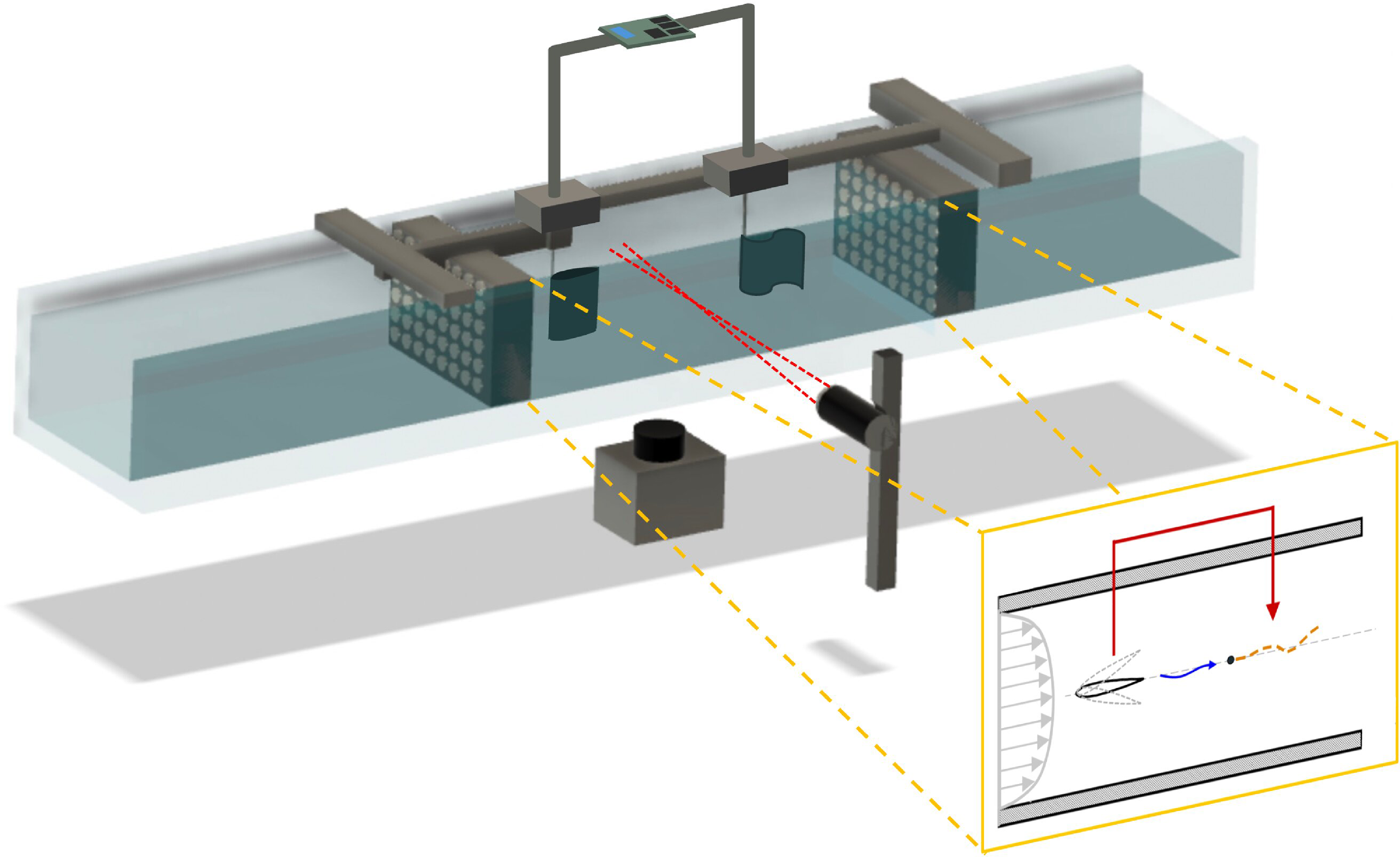
Fish schooling is commonly observed in several species and habitats (Pavlov et al. Reference Pavlov and Kasumyan2000; Filella et al. Reference Filella, Nadal, Sire, Kanso and Eloy2018; Pitcher, Reference Pitcher2001). Fish coordinate their swimming in terms of distance and speed, maintaining different spatial formations (Ashraf et al. Reference Ashraf, Bradshaw, Ha, Halloy, Godoy-Diana and Thiria2017; De Bie et al. Reference De Bie, Manes and Kemp2020; Saadat et al. Reference Saadat, Berlinger, Sheshmani, Nagpal, Lauder and Haj-Hariri2021; Weihs, Reference Weihs1973). Schooling may offer an overall reduced cost of swimming to the entire group (Ashraf et al. Reference Ashraf, Bradshaw, Ha, Halloy, Godoy-Diana and Thiria2017; Liao et al. Reference Liao, Beal, Lauder and Triantafyllou2003; Marras et al. Reference Marras, Killen, Lindström, McKenzie, Steffensen and Domenici2015) and provide advantages in searching for food or route, mating and defending oneself against predators (Landeau & Terborgh, Reference Landeau and Terborgh1986; Larsson, Reference Larsson2012; Major, Reference Major1978; Pitcher et al. Reference Pitcher, Magurran and Winfield1982). When swimming in schools, fish interact via different sensory pathways, including hydrodynamic, visual and acoustic, as illustrated schematically in Figure 1a for a fish pair (Weihs, Reference Weihs1973; Ladich & Winkler, Reference Ladich and Winkler2017; Arnold, Reference Arnold1969; Hyacinthe et al. Reference Hyacinthe, Attia and Rétaux2019; Kasumyan, Reference Kasumyan2004; Li et al. Reference Li, Nagy, Graving, Bak-Coleman, Xie and Couzin2020; Lombana and Porfiri, Reference Lombana and Porfiri2022; Saadat et al. Reference Saadat, Berlinger, Sheshmani, Nagpal, Lauder and Haj-Hariri2021; Thandiackal & Lauder, Reference Thandiackal and Lauder2023). Fish schooling is the result of complex integration of information from an array of sensory pathways. However, disentangling the role of each sensory pathway, segregated from the others, is an open question.
In this work, we focus on a subsystem of a fish school consisting of two fish swimming in line against a flow inside a channel. Our goal is to identify causal interactions between the fish in the presence of multiple distinct modes of interaction. To achieve this goal, we design a robotic platform with an actuated airfoil and a compliant flag that simulates two fish swimming in line against a flow. As shown in Figure 1b, the pitching motion of the upstream airfoil sheds vortices in the flow that interact with the downstream flag, which flaps in response to these flow disturbances. This represents a unidirectional hydrodynamic interaction similar to that observed in fish swimming in line (Porfiri et al. Reference Porfiri, Karakaya, Sattanapalle and Peterson2021; Thandiackal & Lauder, Reference Thandiackal and Lauder2023). The use of the compliant flag downstream allows for a larger response to the vortices and a potentially stronger hydrodynamic coupling than that produced by an airfoil pitching downstream, as previously studied by others (Kurt & Moored, Reference Kurt and Moored2018; Rival et al. Reference Rival, Hass and Tropea2011; Zhang et al. Reference Zhang, Rosen, Peterson and Porfiri2018). An electromechanical coupling between the airfoil and the flag is used to incorporate an additional unidirectional interaction pathway from the upstream to the downstream body, portraying, for instance, the effect of visual interaction. The potential of robotic set-ups for the study of hydrodynamic interactions in fish schools has been demonstrated in several studies (Ko et al. Reference Ko, Lauder and Nagpal2023; Lauder et al. Reference Lauder, Lim, Shelton, Witt, Anderson and Tangorra2011; Li et al. Reference Li, Nagy, Graving, Bak-Coleman, Xie and Couzin2020; Marras and Porfiri, Reference Marras and Porfiri2012; Thandiackal & Lauder, Reference Thandiackal and Lauder2023; Zhang et al. Reference Zhang, Krasner, Peterson and Porfiri2019). Overall, our experimental set-up creates a controlled environment that incorporates distinct interaction pathways between two fish-like bodies positioned in line.
In order to study the influence of the upstream body on the downstream one, we employ the information-theoretic measure of transfer entropy (Schreiber, Reference Schreiber2000). Transfer entropy is a measure of asymmetry in the interaction of two coupled stochastic processes (Bossomaier et al. Reference Bossomaier, Barnett, Harré and Lizier2016). It is emerging as the statistical approach of choice for studying pairwise interactions in complex systems in such wide-ranging fields as climate science, collective behaviour, neuroscience and finance (Staniek & Lehnertz, Reference Staniek and Lehnertz2008; Butail et al. Reference Butail, Mwaffo and Porfiri2016; Stetter et al. Reference Stetter, Battaglia, Soriano and Geisel2012; Vicente et al. Reference Vicente, Wibral, Lindner and Pipa2011; Shaffer & Abaid, Reference Shaffer and Abaid2020; Camacho et al. Reference Camacho, Romeu and Ruiz-Marin2021; Campuzano et al. Reference Campuzano, De Santis, Pavón-Carrasco, Osete and Qamili2018; Hlinka et al. Reference Hlinka, Hartman, Vejmelka, Runge, Marwan, Kurths and Paluš2013; Valentini et al. Reference Valentini, Pavlic, Walker, Pratt, Biro and Sasaki2021; Sandoval Jr, Reference Sandoval2014). Previous work by Zhang et al. (Reference Zhang, Rosen, Peterson and Porfiri2018) investigated the use of transfer entropy to elucidate the causal relationships between two tandem pitching airfoils communicating through the flow. The study involved interaction only via the hydrodynamic pathway and the response of the rigid airfoil downstream was limited. To address these limitations and to disentangle multiple sensory pathways, in this work: (i) we study the influence of a pitching airfoil on a compliant flag with multiple coexisting pathways of interaction – hydrodynamic and electromechanical, and (ii) we further conduct flow measurements to acquire information regarding the hydrodynamic pathway. We combine transfer entropy with experimental diagnostics/measurements to segregate the individual pathways of interaction from the airfoil to the flag. We do so by conditioning transfer entropy on the flow-related information/measurement. This conditional transfer entropy is demonstrated to reduce the overall interaction between the airfoil and the flag and predict the appropriate time delays of the interaction pathways.
The remainder of the paper is organised as follows. In § 2, the experimental set-up is described in detail, followed by a discussion of the three specific experimental conditions examined in this work. This section further details the experimental measurements and movement tracking involved together with the proposed statistical measures for detecting interactions along different pathways by analysing the experimental data. § 3 first demonstrates the processing of the recorded time series from experiments to prepare them for the transfer entropy analysis. Following this, the results and analyses of each of the three experimental cases are described. Finally, the main conclusions drawn from this study are outlined in § 4.
2. Methods
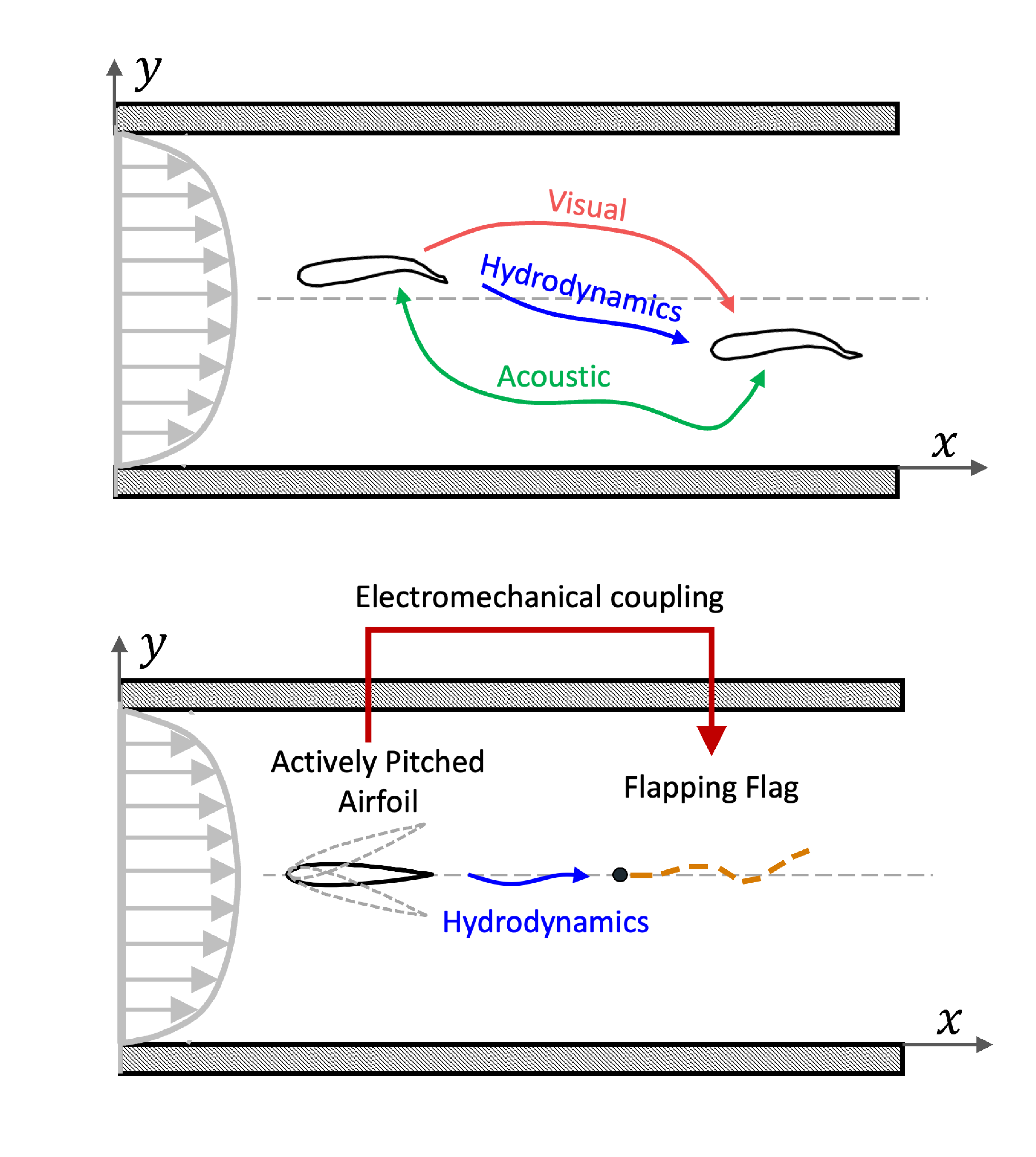
Figure 1. Schematic representation of the proposed experimental approach. Top figure shows two fish swimming in a water channel and interacting via three distinct sensory pathways – visual, hydrodynamic and acoustic. Bottom figure shows a mechanical set-up that simulates the two fish swimming steadily against a channel flow, constituted by an actively pitching airfoil upstream and a compliant flag downstream. The airfoil influences the flag via two separate interaction pathways – hydrodynamics and electromechanical.
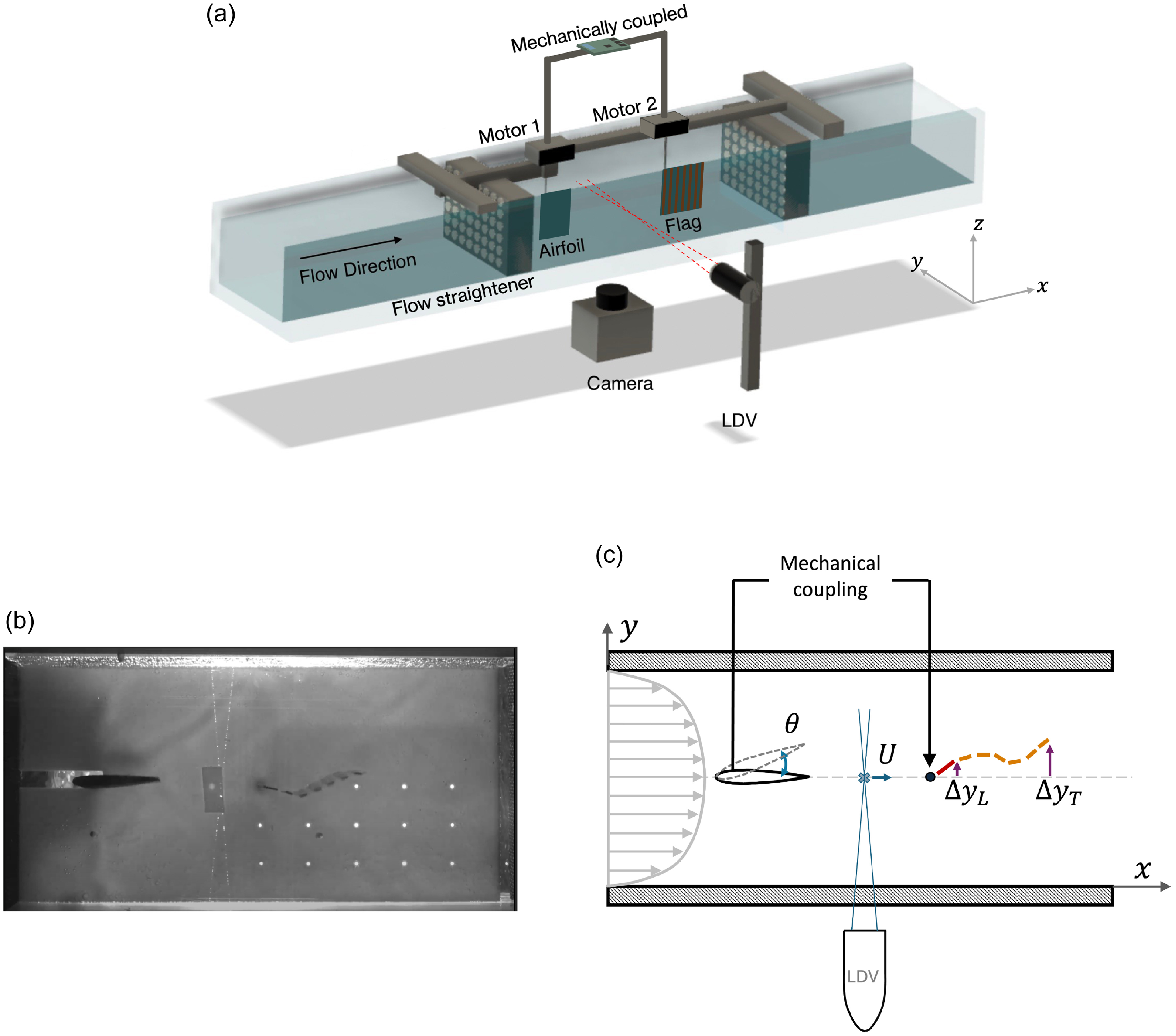
Figure 2. Experimental set-up in a water channel: (a) three-dimensional view of the test section with an upstream airfoil and a downstream flag, a camera recording the bottom view of the test section, and laser Doppler velocimetry system measuring the streamwise flow velocity between the airfoil and the flag; (b) two-dimensional view of the test section from the bottom of the water channel as captured by the camera; and (c) a schematic representation of the two-dimensional test section with the tracked variables marked.
2.1. Experimental design
Experiments were conducted in an open water channel from Engineering Laboratory Design, Inc. The test section, shown in Figure 2(a), is $29 \; \mathrm{cm}$
long with a rectangular cross-section of dimension
$29 \; \mathrm{cm}$
long with a rectangular cross-section of dimension $10 \; \mathrm{cm} \times 15 \; \mathrm{cm}$
. The incoming flow was conditioned (straightening and reducing turbulence intensity) by passing it through a honeycomb section. An extruded airfoil was positioned towards the upstream end of the test section and a compliant flag was positioned in line with the airfoil and
$10 \; \mathrm{cm} \times 15 \; \mathrm{cm}$
. The incoming flow was conditioned (straightening and reducing turbulence intensity) by passing it through a honeycomb section. An extruded airfoil was positioned towards the upstream end of the test section and a compliant flag was positioned in line with the airfoil and $10.4 \; \mathrm{cm}$
downstream from its leading edge.
$10.4 \; \mathrm{cm}$
downstream from its leading edge.
The airfoil was 3D-printed with a NACA $0012$
cross-sectional geometry. It had a chord length of
$0012$
cross-sectional geometry. It had a chord length of $c=5 \; \mathrm{cm}$
, spanwise length of
$c=5 \; \mathrm{cm}$
, spanwise length of $6.9 \; \mathrm{cm}$
and was designed to undergo a pitching motion about a pivot shaft located at
$6.9 \; \mathrm{cm}$
and was designed to undergo a pitching motion about a pivot shaft located at $20\%$
of the airfoil chord while remaining stationary otherwise. The airfoil’s pitching motion was actively regulated by a servo-motor controlled by an Arduino Uno microcontroller board, programmed with the Arduino
$20\%$
of the airfoil chord while remaining stationary otherwise. The airfoil’s pitching motion was actively regulated by a servo-motor controlled by an Arduino Uno microcontroller board, programmed with the Arduino $1.8.19$
software package. The airfoil was subjected to continuous low-amplitude periodic pitching interspersed with sudden random startling motions of higher amplitude.
$1.8.19$
software package. The airfoil was subjected to continuous low-amplitude periodic pitching interspersed with sudden random startling motions of higher amplitude.
A flag with dimensions of $6.98 \; \mathrm{cm}$
length
$6.98 \; \mathrm{cm}$
length $\times \; 6.9 \; \mathrm{cm}$
height was constructed. The design included: a
$\times \; 6.9 \; \mathrm{cm}$
height was constructed. The design included: a $1 \; \mathrm{mm}$
diameter
$1 \; \mathrm{mm}$
diameter $69 \; \mathrm{mm}$
long flag pole; a Mylar sheet that covered the entire flag area; two
$69 \; \mathrm{mm}$
long flag pole; a Mylar sheet that covered the entire flag area; two $7 \; \mathrm{mm} \times 69 \; \mathrm{mm}$
copper strips anchored to the pole and to the two sides of the Mylar sheet forming the first fixed rib (leading rib); and six pairs of
$7 \; \mathrm{mm} \times 69 \; \mathrm{mm}$
copper strips anchored to the pole and to the two sides of the Mylar sheet forming the first fixed rib (leading rib); and six pairs of $4\; \mathrm{mm} \times 69 \; \mathrm{mm}$
copper strips firmly fastened to either side of the Mylar sheet forming the remaining six ribs of the flag with
$4\; \mathrm{mm} \times 69 \; \mathrm{mm}$
copper strips firmly fastened to either side of the Mylar sheet forming the remaining six ribs of the flag with $5.5 \; \mathrm{mm}$
gaps between two ribs. The flag’s design, particularly its mass density and bending stiffness, guaranteed flexibility and capacity to flap (Giacomello & Porfiri, Reference Giacomello and Porfiri2011). It also prevented torsional motion of the flag along the streamwise and spanwise axes, effectively reducing its motion to two dimensions and led to flutter instability of the flag at very high flow speeds (
$5.5 \; \mathrm{mm}$
gaps between two ribs. The flag’s design, particularly its mass density and bending stiffness, guaranteed flexibility and capacity to flap (Giacomello & Porfiri, Reference Giacomello and Porfiri2011). It also prevented torsional motion of the flag along the streamwise and spanwise axes, effectively reducing its motion to two dimensions and led to flutter instability of the flag at very high flow speeds ( $\geq 0.5 \; \mathrm{m/s}$
). The flag was securely positioned
$\geq 0.5 \; \mathrm{m/s}$
). The flag was securely positioned $5.4 \; \mathrm{cm}$
downstream from the airfoil trailing edge. In the presence of a flow, a major portion of the flag downstream of the first anchored rib was free to flap passively in response to the fluctuating flow structures produced by the upstream airfoil’s pitching. The first anchored rib of the flag was actuated to undergo periodic pitching motion, similar to the airfoil, using a second servo-motor controlled by the same microcontroller board.
$5.4 \; \mathrm{cm}$
downstream from the airfoil trailing edge. In the presence of a flow, a major portion of the flag downstream of the first anchored rib was free to flap passively in response to the fluctuating flow structures produced by the upstream airfoil’s pitching. The first anchored rib of the flag was actuated to undergo periodic pitching motion, similar to the airfoil, using a second servo-motor controlled by the same microcontroller board.
In all experiments, the airfoil’s periodic pitching motion was maintained at a frequency of $3 \; \mathrm{Hz}$
and amplitude of
$3 \; \mathrm{Hz}$
and amplitude of $15^\circ$
. Additionally, we included a random startling motion of
$15^\circ$
. Additionally, we included a random startling motion of $40^\circ$
angular deflection. The direction of the startle was chosen randomly and the time duration between two consecutive startles were sampled from a uniform random distribution in
$40^\circ$
angular deflection. The direction of the startle was chosen randomly and the time duration between two consecutive startles were sampled from a uniform random distribution in $5 \pm 1.5 \; \mathrm{s}$
. Experiments were conducted in the channel with static water (no flow) as well as with water flowing steadily through the channel. The inflow speed in the test section was maintained at
$5 \pm 1.5 \; \mathrm{s}$
. Experiments were conducted in the channel with static water (no flow) as well as with water flowing steadily through the channel. The inflow speed in the test section was maintained at $U_0=0.394 \; \mathrm{m/s}$
at the centreline (recorded using laser Doppler velocimetry described later in the section). This represents a chord-based Reynolds number of
$U_0=0.394 \; \mathrm{m/s}$
at the centreline (recorded using laser Doppler velocimetry described later in the section). This represents a chord-based Reynolds number of $Re = U_0 c / \nu = 21850$
and kinematic viscosity of water at room temperature is
$Re = U_0 c / \nu = 21850$
and kinematic viscosity of water at room temperature is $\nu \approx 9 \times 10^{-7} \mathrm{m^2/s}$
.
$\nu \approx 9 \times 10^{-7} \mathrm{m^2/s}$
.
2.2. Experimental cases
We performed experiments for the following conditions:
-
(i) Hydrodynamic interaction: to study the effect of hydrodynamic interaction between the airfoil and the flag, the flow channel was operated at a steady flow speed. The airfoil was subjected to periodic pitching motion superimposed with startling motions at random time intervals. The flag was not actuated and underwent flapping motion in response to the vortices generated by the upstream pitching airfoil.
-
(ii) Hydrodynamic + electromechanical interaction: to obtain hydrodynamic and electromechanical interaction between the airfoil and the flag, we maintained a steady flow of water in the channel and periodic pitching along with random startles in the airfoil. In addition, the first rib of the flag was electromechanically coupled to the airfoil motion. This was done by imposing the airfoil’s pitching and startling motion on the flag’s leading rib at a specific time delay ( $\Delta _{AF}=$
$0.1 \; \mathrm{s}, 0.3 \; \mathrm{s}$
) along with a certain degree of random noise. The noise was introduced in the form of additional ‘noise startles’ with a mean time gap of
$\Delta _{no}=0.04 \mathrm{s}, 0.08 \mathrm{s}$
.
$\Delta _{AF}=$
$0.1 \; \mathrm{s}, 0.3 \; \mathrm{s}$
) along with a certain degree of random noise. The noise was introduced in the form of additional ‘noise startles’ with a mean time gap of
$\Delta _{no}=0.04 \mathrm{s}, 0.08 \mathrm{s}$
. -
(iii) Electromechanical interaction: to study the case of only electromechanical interaction between the airfoil and the flag, experiments were conducted in static water. A periodic pitching motion interspersed with random startles was imposed on the airfoil and also on the flag with a time lag and added noise, similar to the previous case.


2.3. Measurement and tracking
Two forms of measurement were conducted during the experiments:
-
(i) Camera recording: a high-resolution camera (Point Grey Flea 3 USB camera; Point Grey, Richmond, Canada) was utilised to capture a two-dimensional view of the full test section (
$29 \; \mathrm{cm} \times 15 \; \mathrm{cm}$
), including the movement of the airfoil and the flag, as observed from below the water channel (Figure 2b). To document these sequences, the open-source software package, OBS Studio, was employed. The experimental footage was recorded at a resolution of
$1920 \times 1080$
pixels and at a rate of
$60$
frames/s. Before experimental trials, the camera was calibrated by capturing and processing a video with a length-scale marked ruler in the test section. Correcting for any scale or distortion in the camera recordings, the calibration process enabled precise measurement of all movements within the test section. -
(ii) Laser Doppler velocimetry: high spatial and temporal resolution fluid flow velocity measurements were made using the non-invasive laser Doppler velocimetry (LDV) technique (Foreman et al. Reference Foreman, George and Lewis1965; Kalkert & Kayser, Reference Kalkert and Kayser2006). An optical technique that measures the velocity of passive tracer particles in a flow by analyzing the frequency shift of the laser light scattered by the moving particles. A single-component LDV system (Dantec Dynamics, Skovlunde, Hovedstaden, Denmark) was used to measure the instantaneous streamwise component of the flow velocity,
$U$
, at the channel centreline
$3 \; \mathrm{cm}$
downstream from the trailing edge of the airfoil. The BSA Flow software was used to record the LDV measurement over the course of each experiment. As LDV is dependent on light scattered by particles passing through the measurement volume, the measurement of
$U$
was not uniformly spaced in time. Polyamide particles were added to the flow to increase the sampling rate.


During each experiment, videos of the test section view and LDV measurement of flow velocity were recorded for a duration of $180 \; \mathrm{s}$
. The recorded videos were processed to track the movements of the airfoil and flag by a program developed in MATLAB R2021b, using utilities available in its image processing toolbox. Specifically, the following quantities were tracked: the pitching angle of the airfoil,
$180 \; \mathrm{s}$
. The recorded videos were processed to track the movements of the airfoil and flag by a program developed in MATLAB R2021b, using utilities available in its image processing toolbox. Specifically, the following quantities were tracked: the pitching angle of the airfoil, $\theta (t)$
, the spanwise deflection of the leading rib of the flag,
$\theta (t)$
, the spanwise deflection of the leading rib of the flag, $\Delta y_{L}(t)$
, and the spanwise deflection of the trailing rib of the flag,
$\Delta y_{L}(t)$
, and the spanwise deflection of the trailing rib of the flag, $\Delta y_{T}(t)$
, as marked in Figure 2c.
$\Delta y_{T}(t)$
, as marked in Figure 2c.
2.4. Information-theoretic measures
Information theory is rooted in the concept of Shannon entropy (Shannon, Reference Shannon1948) that encodes the uncertainty or information content of a random variable $X$
$X$
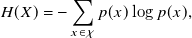 \begin{equation} H(X) = - \sum _{x \in \chi }p(x)\log p(x), \end{equation}
where $p(x)$
is the probability of an outcome
$p(x)$
is the probability of an outcome $x$
in the set of all possible outcomes (
$x$
in the set of all possible outcomes ( $\chi$
) of
$\chi$
) of $X$
; we use base
$X$
; we use base $2$
for the logarithms throughout the manuscript so that entropy is measured in bits. Similarly, the joint entropy of two random variables
$2$
for the logarithms throughout the manuscript so that entropy is measured in bits. Similarly, the joint entropy of two random variables $X$
and
$X$
and $Y$
is given by
$Y$
is given by
 \begin{equation} H(X,Y) =- \sum _{x \in \chi, y \in \gamma } p(x,y)\log p(x,y), \end{equation}
where $\gamma$
is the set of all possible outcomes of
$\gamma$
is the set of all possible outcomes of $Y$
. The conditional entropy of
$Y$
. The conditional entropy of $X$
given
$X$
given $Y$
is
$Y$
is
 \begin{equation} H(X|Y) =- \sum _{x \in \chi, y \in \gamma } p(x,y)\log p(x|y). \end{equation}
For two discrete-time stationary random processes, $X=\{X_n\}_{n=1}^{\infty }$
and
$X=\{X_n\}_{n=1}^{\infty }$
and $Y=\{Y_n\}_{n=1}^{\infty }$
, where
$Y=\{Y_n\}_{n=1}^{\infty }$
, where $n$
is the time index, the influence (Wiener, Reference Wiener1956) of
$n$
is the time index, the influence (Wiener, Reference Wiener1956) of $X$
on
$X$
on $Y$
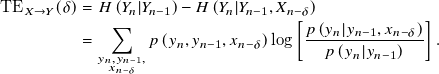
can be discerned by utilising transfer entropy (Schreiber, Reference Schreiber2000; Wibral et al. Reference Wibral, Pampu, Priesemann, Siebenhühner, Seiwert, Lindner, Lizier, Vicente and Hayasaka2013), defined as follows:
$Y$
can be discerned by utilising transfer entropy (Schreiber, Reference Schreiber2000; Wibral et al. Reference Wibral, Pampu, Priesemann, Siebenhühner, Seiwert, Lindner, Lizier, Vicente and Hayasaka2013), defined as follows:
 \begin{eqnarray} \mathrm{TE}_{X \rightarrow Y}(\delta) & = & H\left (Y_{n}|Y_{n-1}\right) - H\left (Y_{n}|Y_{n-1},X_{n-\delta }\right) \nonumber \\ & = & \sum _{ \substack {y_{n}, y_{n-1},\\x_{n-\delta }} } p\left (y_{n}, y_{n-1}, x_{n-\delta }\right) \log \left [ \frac {p\left (y_{n}| y_{n-1}, x_{n-\delta }\right)}{p\left (y_{n}| y_{n-1}\right)} \right]. \end{eqnarray}
Transfer entropy from $X$
to
$X$
to $Y$
is the reduction in uncertainty of target
$Y$
is the reduction in uncertainty of target $Y_n$
given its recent past,
$Y_n$
given its recent past, $Y_{n-1}$
, due to the knowledge of the source’s past state,
$Y_{n-1}$
, due to the knowledge of the source’s past state, $X_{n-\delta }$
. Therefore,
$X_{n-\delta }$
. Therefore, $\mathrm{TE}_{X \rightarrow Y}$
captures the influence of
$\mathrm{TE}_{X \rightarrow Y}$
captures the influence of $X$
on
$X$
on $Y$
with a time lag of
$Y$
with a time lag of $\delta$
time steps. Likewise,
$\delta$
time steps. Likewise, $\mathrm{TE}_{Y \rightarrow X}$
quantifies the influence of
$\mathrm{TE}_{Y \rightarrow X}$
quantifies the influence of $Y$
on
$Y$
on $X$
. When
$X$
. When $X$
and
$X$
and $Y$
have an asymmetric causal interaction, net transfer entropy,
$Y$
have an asymmetric causal interaction, net transfer entropy, $\mathrm{net \; TE}_{X \rightarrow Y} = \mathrm{TE}_{X \rightarrow Y} - \mathrm{TE}_{Y \rightarrow X}$
, can be used to indicate the predominant direction of influence.
$\mathrm{net \; TE}_{X \rightarrow Y} = \mathrm{TE}_{X \rightarrow Y} - \mathrm{TE}_{Y \rightarrow X}$
, can be used to indicate the predominant direction of influence.
If an additional random process $Z_{n}$
is related to the
$Z_{n}$
is related to the $X$
-
$X$
- $Y$
dynamics, we quantify the causal dependence through
$Y$
dynamics, we quantify the causal dependence through
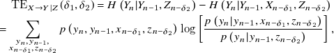 \begin{eqnarray} \mathrm{TE}_{X \rightarrow Y | Z}(\delta _1,\delta _2) = H\left (Y_{n}|Y_{n-1},Z_{n-\delta _2}\right) - H\left (Y_{n}|Y_{n-1},X_{n-\delta _1},Z_{n-\delta _2}\right) \nonumber \\ = \sum _{\substack {y_{n}, y_{n-1},\\x_{n-\delta _1}, z_{n-\delta _2}}} p\left (y_{n}, y_{n-1}, x_{n-\delta _1},z_{n-\delta _2}\right) \log \left [ \frac {p\left (y_{n}| y_{n-1}, x_{n-\delta _1},z_{n-\delta _2}\right)}{p\left (y_{n}| y_{n-1},z_{n-\delta _2}\right)} \right], \end{eqnarray}
which is referred to as conditional transfer entropy (Sun & Bollt, Reference Sun and Bollt2014). Conditional transfer entropy from $X$
to
$X$
to $Y$
conditioned on
$Y$
conditioned on $Z$
represents the influence of the past of
$Z$
represents the influence of the past of $X$
(delay of
$X$
(delay of $\delta _1$
steps) on current
$\delta _1$
steps) on current $Y$
, accounting for the knowledge of its own immediate past as well as the past of
$Y$
, accounting for the knowledge of its own immediate past as well as the past of $Z$
at a delay of
$Z$
at a delay of $\delta _2$
steps.
$\delta _2$
steps.
Accurate estimation of these measures requires computation of up to a four-dimensional joint probability mass function (PMF), which can be challenging to estimate with a finite number of data samples. To circumvent this issue, we symbolised each time series using a dynamics-based approach (Porfiri & Marín, Reference Porfiri and Marín2017) with an embedding dimension of $m=2$
. This approach converts a time series (
$m=2$
. This approach converts a time series ( $X_n$
) to symbolised time series (
$X_n$
) to symbolised time series ( ${\pi _X}_n$
) of
${\pi _X}_n$
) of $1$
and
$1$
and $0$
based on whether the value is increasing or decreasing, respectively, at a given time instant. The estimated PMF of the symbolised time series is accurate and robust to noise since the finite dataset is split between only two bins. Once the joint PMFs are estimated, transfer entropy and conditional transfer entropy are obtained using equations (2.4) and (2.5).
$0$
based on whether the value is increasing or decreasing, respectively, at a given time instant. The estimated PMF of the symbolised time series is accurate and robust to noise since the finite dataset is split between only two bins. Once the joint PMFs are estimated, transfer entropy and conditional transfer entropy are obtained using equations (2.4) and (2.5).
Once the transfer entropy is estimated from experimental data, it is pertinent to conduct statistical testing in order to infer whether the suggested causal influence is statistically significant. For transfer entropy, $\mathrm{TE}_{X \rightarrow Y}$
, we generated a surrogate distribution of the transfer entropy by following a random permutation test. We randomly shuffled the source time series
$\mathrm{TE}_{X \rightarrow Y}$
, we generated a surrogate distribution of the transfer entropy by following a random permutation test. We randomly shuffled the source time series $\{{X}_n\}$
, keeping the target time series unchanged, to maintain the link between it
$\{{X}_n\}$
, keeping the target time series unchanged, to maintain the link between it $\{{Y}_n\}$
and its past
$\{{Y}_n\}$
and its past $\{{Y}_{n-1}\}$
. We computed the corresponding transfer entropy to generate
$\{{Y}_{n-1}\}$
. We computed the corresponding transfer entropy to generate $N_{\mathrm{sur}}=10000$
samples for the surrogate distribution. To test if conditioning on
$N_{\mathrm{sur}}=10000$
samples for the surrogate distribution. To test if conditioning on $Z$
significantly reduces transfer entropy,
$Z$
significantly reduces transfer entropy, $\mathrm{TE}_{X \rightarrow Y|Z}$
, we generated a surrogate distribution by shuffling the
$\mathrm{TE}_{X \rightarrow Y|Z}$
, we generated a surrogate distribution by shuffling the $Z$
time series
$Z$
time series $N_{\mathrm{sur}}=10000$
times, while maintaining the link between the source and target (
$N_{\mathrm{sur}}=10000$
times, while maintaining the link between the source and target ( $X$
-
$X$
- $Y$
). The transfer entropy (or conditional transfer entropy) value was considered to be significant if the value was in the right (or left) tail of the surrogate distribution with a p-value smaller than
$Y$
). The transfer entropy (or conditional transfer entropy) value was considered to be significant if the value was in the right (or left) tail of the surrogate distribution with a p-value smaller than $0.05$
. This enabled us to assess: (i) whether transfer entropy from a source to a target is significantly greater than that between a random source to the same target, and (ii) whether conditioning transfer entropy on a relevant variable
$0.05$
. This enabled us to assess: (i) whether transfer entropy from a source to a target is significantly greater than that between a random source to the same target, and (ii) whether conditioning transfer entropy on a relevant variable $Z$
reduced the transfer entropy as compared with conditioning on a random unrelated time series.
$Z$
reduced the transfer entropy as compared with conditioning on a random unrelated time series.
3. Results
In this section, we analyse the experimental observations using transfer entropy-based methods. First, the recorded time series of movements and flow velocity are illustrated, followed by a discussion on the processing of the time series prior to conducting information-theoretic analysis. Then, results of the three experimental conditions of interaction between the airfoil and the flag outlined in § 2.2 are discussed individually.
3.1. Pre-processing of time series
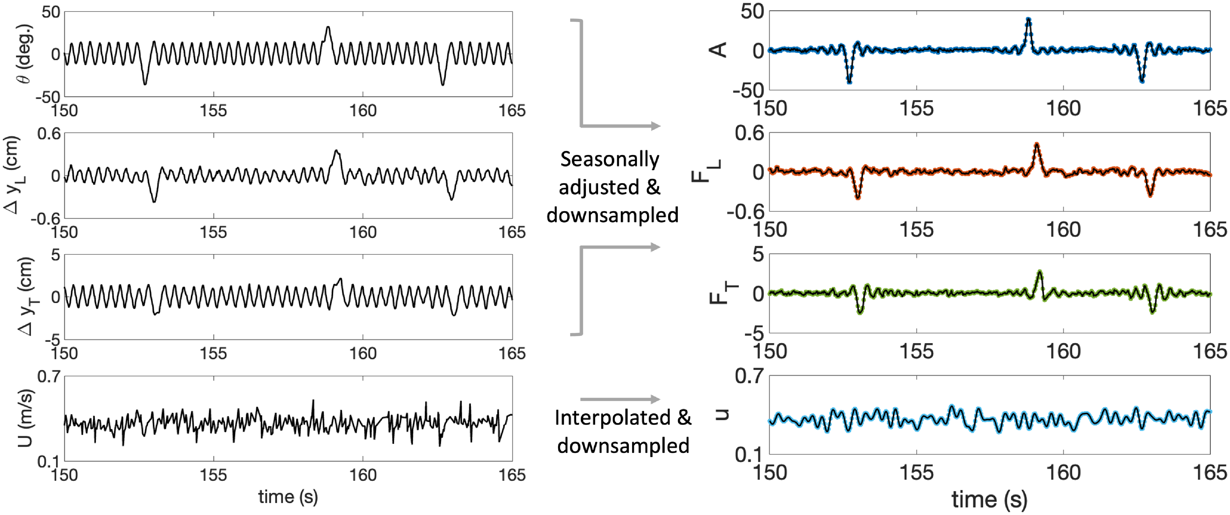
Figure 3. Portion of the raw time series (left) and corresponding processed time series (right) of (from top to bottom): airfoil pitching angle (raw: $\theta$
and processed:
$\theta$
and processed: $A$
), flag’s leading rib deflection (
$A$
), flag’s leading rib deflection ( $\Delta y_{L}$
and
$\Delta y_{L}$
and $F_{L}$
), flag’s trailing rib deflection (
$F_{L}$
), flag’s trailing rib deflection ( $\Delta y_{T}$
and
$\Delta y_{T}$
and $F_{T}$
) and streamwise flow speed recorded by LDV (
$F_{T}$
) and streamwise flow speed recorded by LDV ( $U$
and
$U$
and $u$
). The coloured dots in the plots on the right represent the downsampled time series used for symbolisation and later for transfer entropy analysis.
$u$
). The coloured dots in the plots on the right represent the downsampled time series used for symbolisation and later for transfer entropy analysis.
The experimental measurement and tracking (§ 2.3) yields raw time-series data of the airfoil pitching angle $\theta$
, flag leading rib deflection
$\theta$
, flag leading rib deflection $\Delta y_L$
, flag trailing rib deflection
$\Delta y_L$
, flag trailing rib deflection $\Delta y_T$
and LDV-recorded streamwise flow speed
$\Delta y_T$
and LDV-recorded streamwise flow speed $U$
, as shown in the left panel of Figure 3. The airfoil angle
$U$
, as shown in the left panel of Figure 3. The airfoil angle $\theta$
demonstrates the periodic pitching motion interspersed with high-magnitude startles appearing at random time instants. The flag (both
$\theta$
demonstrates the periodic pitching motion interspersed with high-magnitude startles appearing at random time instants. The flag (both $\Delta y_L$
and
$\Delta y_L$
and $\Delta y_T$
) responds to the unsteady flow vortices generated by the pitching airfoil and demonstrates similar periodic and startling motions as the airfoil, only with a discernible time delay. The instantaneous streamwise flow speed
$\Delta y_T$
) responds to the unsteady flow vortices generated by the pitching airfoil and demonstrates similar periodic and startling motions as the airfoil, only with a discernible time delay. The instantaneous streamwise flow speed $U$
, on the other hand, does not exhibit a periodic behaviour and appears to be relatively more noisy, characteristic of a turbulent flow. Towards preparing the time series for the calculation of the information-theoretic measures, we sought to temporally match all the time series, suppress the effects of measurement noise, and address superfluous periodicity. These goals were pursued through the following steps.
$U$
, on the other hand, does not exhibit a periodic behaviour and appears to be relatively more noisy, characteristic of a turbulent flow. Towards preparing the time series for the calculation of the information-theoretic measures, we sought to temporally match all the time series, suppress the effects of measurement noise, and address superfluous periodicity. These goals were pursued through the following steps.
Seasonal adjustment: the first three time series, $\theta, \Delta y_L$
and
$\theta, \Delta y_L$
and $\Delta y_T$
, were recorded at uniformly spaced frequency of
$\Delta y_T$
, were recorded at uniformly spaced frequency of $60 \; \mathrm{Hz}$
with a distinct seasonality in their behaviour. The periodic pitching helps maintain a continuous interaction between the airfoil and the flag, but it is the random startles and other mechanical noise that sustain the stochastic nature of the time series and is essential in applying statistical methods for causal inference. Therefore, prior to conducting the information-theoretic analysis, the time series must be seasonally adjusted, as commonly done in econometrics (Porfiri et al. Reference Porfiri, Sattanapalle, Nakayama, Macinko and Sipahi2019). We performed a seasonal adjustment on the
$60 \; \mathrm{Hz}$
with a distinct seasonality in their behaviour. The periodic pitching helps maintain a continuous interaction between the airfoil and the flag, but it is the random startles and other mechanical noise that sustain the stochastic nature of the time series and is essential in applying statistical methods for causal inference. Therefore, prior to conducting the information-theoretic analysis, the time series must be seasonally adjusted, as commonly done in econometrics (Porfiri et al. Reference Porfiri, Sattanapalle, Nakayama, Macinko and Sipahi2019). We performed a seasonal adjustment on the $\theta$
,
$\theta$
, $\Delta y_L$
and
$\Delta y_L$
and $\Delta y_T$
time series, employing the multiple seasonal-trend decomposition using LOESS (locally estimated scatterplot smoothing) package in Python 3.9.7 to eliminate the “seasonal” trends in the data. This results in the processed time series of
$\Delta y_T$
time series, employing the multiple seasonal-trend decomposition using LOESS (locally estimated scatterplot smoothing) package in Python 3.9.7 to eliminate the “seasonal” trends in the data. This results in the processed time series of $A$
for the airfoil’s motion,
$A$
for the airfoil’s motion, $F_L$
for the flag’s leading rib motion and
$F_L$
for the flag’s leading rib motion and $F_T$
for the flag’s trailing rib motion as depicted in the right column of Figure 3. Disregarding the oscillations, these time series primarily encapsulate the startling motions. To remove experimental noise linked to mechanical movements or measurements, the time series were downsampled from the recorded
$F_T$
for the flag’s trailing rib motion as depicted in the right column of Figure 3. Disregarding the oscillations, these time series primarily encapsulate the startling motions. To remove experimental noise linked to mechanical movements or measurements, the time series were downsampled from the recorded $60$
frames per second to
$60$
frames per second to $30$
data points per second.
$30$
data points per second.
Interpolation: unlike the image-tracked motion of the airfoil and the flag, $U$
was measured whenever a particle was tracked crossing the LDV measurement volume and was therefore non-uniformly spaced in time (
$U$
was measured whenever a particle was tracked crossing the LDV measurement volume and was therefore non-uniformly spaced in time ( $\sim 15$
data points per second on average). Thus,
$\sim 15$
data points per second on average). Thus, $U$
was interpolated and resampled to obtain a time series
$U$
was interpolated and resampled to obtain a time series $u$
that aligned in time with the uniformly spaced downsampled time series of
$u$
that aligned in time with the uniformly spaced downsampled time series of $A$
,
$A$
, $F_L$
and
$F_L$
and $F_T$
.
$F_T$
.
Symbolisation: finally, these time series were symbolised with an embedding dimension of $m=2$
(as explained in § 2.4) to yield
$m=2$
(as explained in § 2.4) to yield $\pi _A$
,
$\pi _A$
, $\pi _{F_L}$
,
$\pi _{F_L}$
, $\pi _{F_T}$
and
$\pi _{F_T}$
and $\pi _u$
(Figure 4). The symbolised time series were assigned binary values of
$\pi _u$
(Figure 4). The symbolised time series were assigned binary values of $0$
and
$0$
and $1$
, depending on whether it decreased or increased in value from one time step to the next. This results in probability estimation that is more robust to noise. These symbolised time series at a constant time increment of
$1$
, depending on whether it decreased or increased in value from one time step to the next. This results in probability estimation that is more robust to noise. These symbolised time series at a constant time increment of $\Delta t=1/30 \mathrm{s} \approx 0.033$
s were finally used for the information-theoretic analysis. Such a symbolic representation is often adapted in information-theoretic analysis (López et al. Reference López, Matilla-García, Mur and Marín2010; Ruiz-Marin et al. Reference Ruiz-Marin, Matilla-Garcia, García, González-Susillo, Romo-Astorga, González-Pérez, Ruiz and Gayan2010) when the relative change in the time series is more important than the precise values they attain at each time instance.
$\Delta t=1/30 \mathrm{s} \approx 0.033$
s were finally used for the information-theoretic analysis. Such a symbolic representation is often adapted in information-theoretic analysis (López et al. Reference López, Matilla-García, Mur and Marín2010; Ruiz-Marin et al. Reference Ruiz-Marin, Matilla-Garcia, García, González-Susillo, Romo-Astorga, González-Pérez, Ruiz and Gayan2010) when the relative change in the time series is more important than the precise values they attain at each time instance.
3.2. Hydrodynamic interaction
First, we analyse the experimental case of an actively controlled airfoil and passive flag in a steady flow inside the water channel. In this case, the leading rib of the flag remains fixed parallel to the streamwise axis and the airfoil and the flag interact primarily via the flow (hydrodynamic pathway). We compute transfer entropy from the airfoil to the flag’s trailing rib and vice versa using Equation (2.4) and illustrate its variation with the time delay ( $\delta$
) between the airfoil and the flag in Figure 5a. We observe that
$\delta$
) between the airfoil and the flag in Figure 5a. We observe that $\mathrm{TE}_{A \rightarrow F_T}$
is typically higher than
$\mathrm{TE}_{A \rightarrow F_T}$
is typically higher than $\mathrm{TE}_{F_T \rightarrow A}$
at nearly all time lags, suggesting a positive
$\mathrm{TE}_{F_T \rightarrow A}$
at nearly all time lags, suggesting a positive $\mathrm{net \; TE}_{A \rightarrow F_T}$
. This implies that the airfoil has a stronger influence on the flag than the flag has on the airfoil, due to the fact that the compliant flag responds to the vortices shed by the pitching motion of the airfoil. The figure further shows that
$\mathrm{net \; TE}_{A \rightarrow F_T}$
. This implies that the airfoil has a stronger influence on the flag than the flag has on the airfoil, due to the fact that the compliant flag responds to the vortices shed by the pitching motion of the airfoil. The figure further shows that $\mathrm{TE}_{A \rightarrow F_T}$
attains a maximum at a time delay of
$\mathrm{TE}_{A \rightarrow F_T}$
attains a maximum at a time delay of $\delta _0=10 \Delta t \approx 0.33 \; \mathrm{s}$
, consistent with our estimated time taken by the flow (based on the maximum streamwise speed
$\delta _0=10 \Delta t \approx 0.33 \; \mathrm{s}$
, consistent with our estimated time taken by the flow (based on the maximum streamwise speed $U_0$
at the centreline) to reach the flag’s trailing rib from the airfoil’s trailing edge of
$U_0$
at the centreline) to reach the flag’s trailing rib from the airfoil’s trailing edge of $\sim 0.3 \; \mathrm{s}$
.
$\sim 0.3 \; \mathrm{s}$
.
To test the statistical significance of $\mathrm{TE}_{A \rightarrow F_T}(\delta _0)$
against chance, we compare with its surrogate distribution created by randomly shuffling the source time series (
$\mathrm{TE}_{A \rightarrow F_T}(\delta _0)$
against chance, we compare with its surrogate distribution created by randomly shuffling the source time series ( $\pi _A$
)
$\pi _A$
) $N_{\mathrm{sur}}=10\,000$
times while preserving the dynamics of the target (
$N_{\mathrm{sur}}=10\,000$
times while preserving the dynamics of the target ( $\pi _{F_T}$
), as described in § 2.4. The surrogate probability distribution is illustrated in Figure 5b along with the peak value of
$\pi _{F_T}$
), as described in § 2.4. The surrogate probability distribution is illustrated in Figure 5b along with the peak value of $\mathrm{TE}_{A \rightarrow F_T}$
. It is evident that
$\mathrm{TE}_{A \rightarrow F_T}$
. It is evident that $\mathrm{TE}_{A \rightarrow F_T}(\delta _0)$
is higher than chance (
$\mathrm{TE}_{A \rightarrow F_T}(\delta _0)$
is higher than chance ( $p\lt 0.0001$
), suggesting that there exists a causal relationship from the actively actuated upstream airfoil to the passively flapping downstream flag with a time delay of
$p\lt 0.0001$
), suggesting that there exists a causal relationship from the actively actuated upstream airfoil to the passively flapping downstream flag with a time delay of $\sim 0.33 \; \mathrm{s}$
.
$\sim 0.33 \; \mathrm{s}$
.
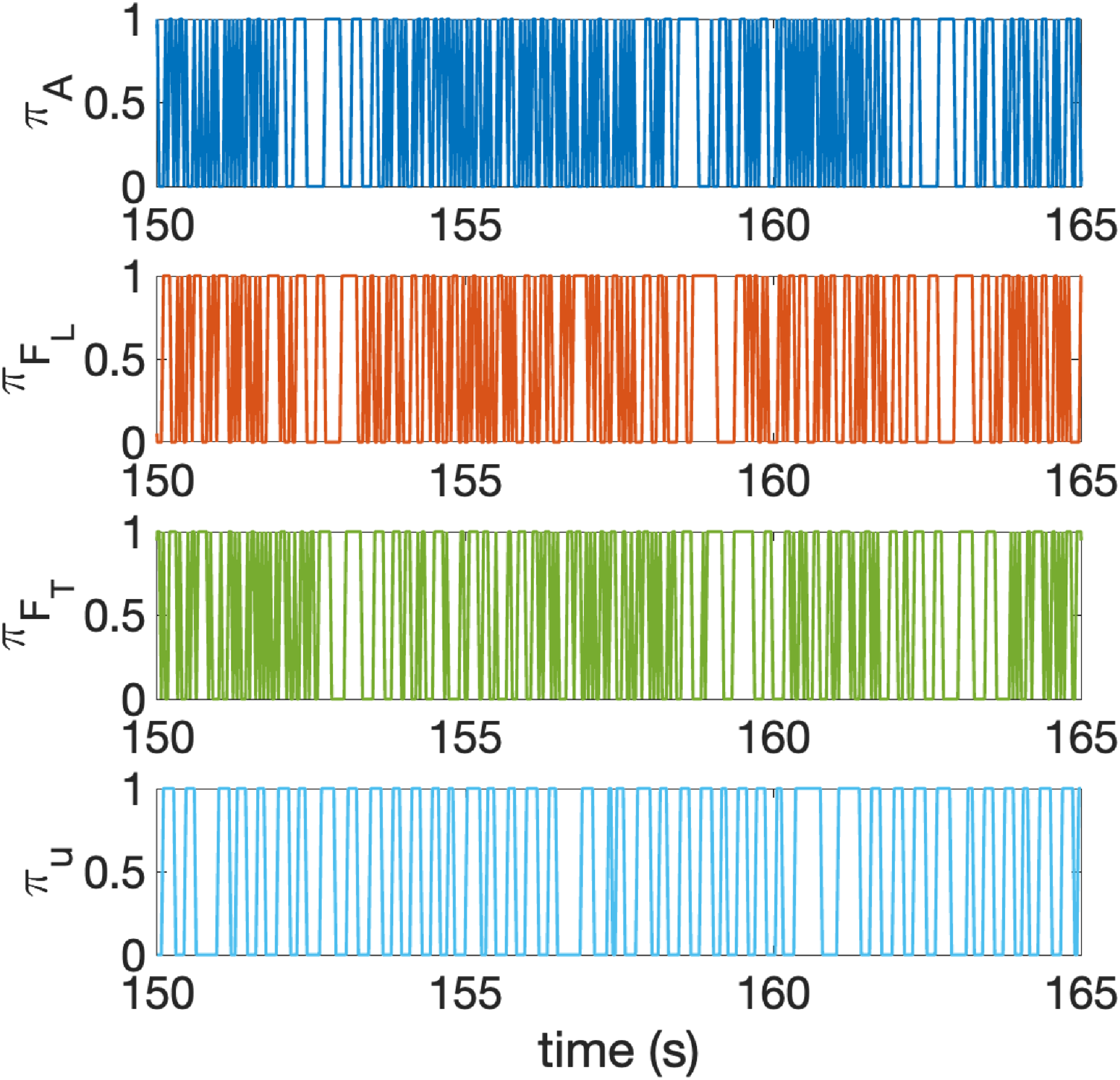
Figure 4. Portion of the symbolised time series of the airfoil pitching angle (raw: $\pi _A$
), flag’s leading rib deflection (
$\pi _A$
), flag’s leading rib deflection ( $\pi _{F_{L}}$
), flag’s trailing rib deflection (
$\pi _{F_{L}}$
), flag’s trailing rib deflection ( $\pi _{F_{T}}$
) and streamwise flow speed recorded by LDV (
$\pi _{F_{T}}$
) and streamwise flow speed recorded by LDV ( $\pi _u$
), directly used for the transfer entropy analysis.
$\pi _u$
), directly used for the transfer entropy analysis.
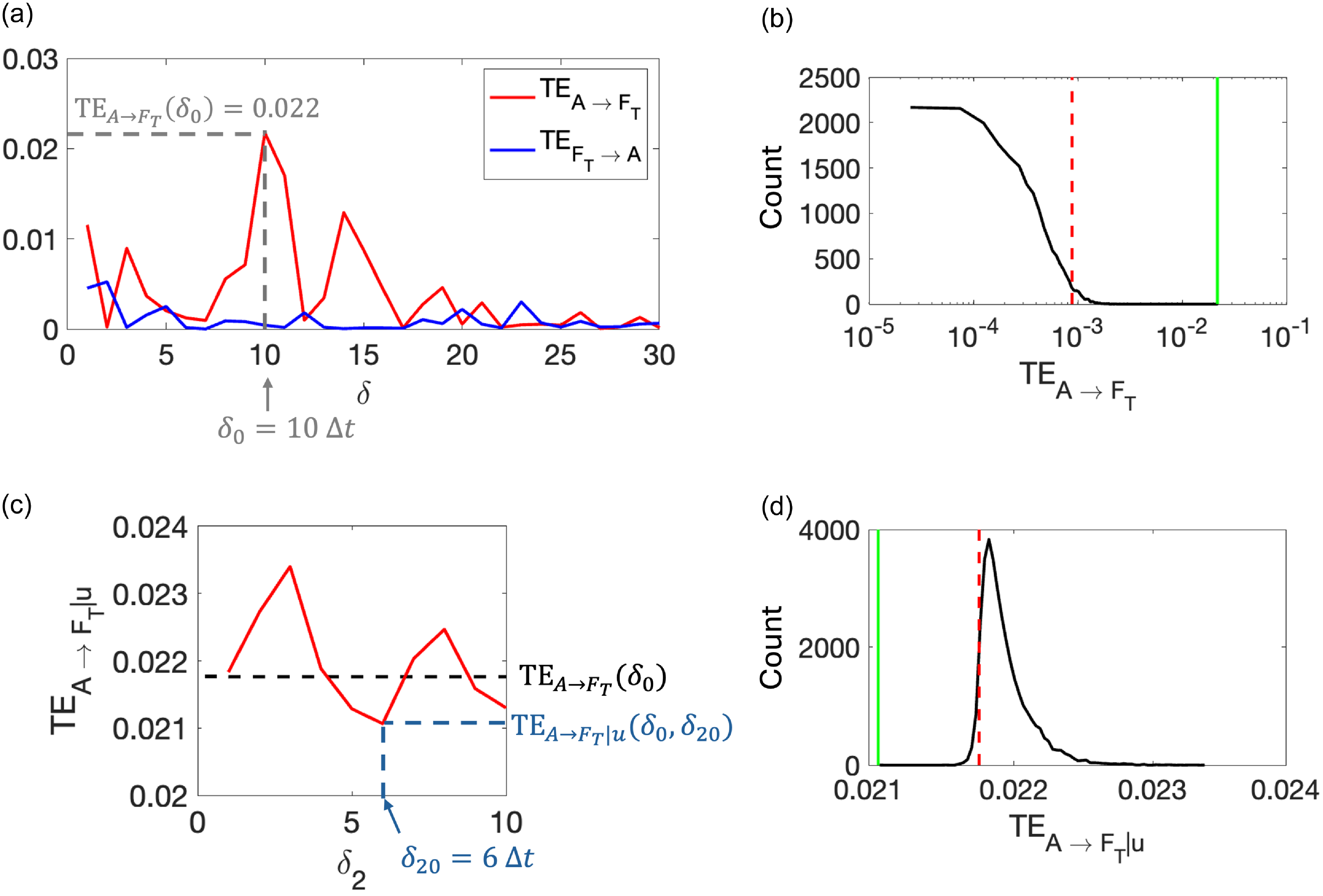
Figure 5. Analysis of experiments with only hydrodynamic interaction: (a) transfer entropy from airfoil to trailing rib of the flag ( $\mathrm{TE}_{A \rightarrow F_T}$
) and from flag to airfoil (
$\mathrm{TE}_{A \rightarrow F_T}$
) and from flag to airfoil ( $\mathrm{TE}_{F_T \rightarrow A}$
) for different delays
$\mathrm{TE}_{F_T \rightarrow A}$
) for different delays $\delta$
between
$\delta$
between $A$
and
$A$
and $F_T$
. Peak
$F_T$
. Peak $\mathrm{TE}_{A \rightarrow F_T}$
is observed at a delay of
$\mathrm{TE}_{A \rightarrow F_T}$
is observed at a delay of $\delta _0=10\Delta t$
. At delay
$\delta _0=10\Delta t$
. At delay $\delta _0$
, (c) conditional transfer entropy from airfoil to flag conditioned on streamwise flow speed,
$\delta _0$
, (c) conditional transfer entropy from airfoil to flag conditioned on streamwise flow speed, $\mathrm{TE}_{A \rightarrow F_T| u}(\delta _0,\delta _2)$
, as a function of time-delay (
$\mathrm{TE}_{A \rightarrow F_T| u}(\delta _0,\delta _2)$
, as a function of time-delay ( $\delta _2$
) between
$\delta _2$
) between $u$
and
$u$
and $F_T$
. Minimum
$F_T$
. Minimum $\mathrm{TE}_{A \rightarrow F_T| u}$
is observed at delay
$\mathrm{TE}_{A \rightarrow F_T| u}$
is observed at delay $\delta _{20}=6\Delta t$
. Statistical tests: (b)
$\delta _{20}=6\Delta t$
. Statistical tests: (b) $\mathrm{TE}_{A \rightarrow F_T}(\delta _0)$
with respect to its surrogate distribution and (d)
$\mathrm{TE}_{A \rightarrow F_T}(\delta _0)$
with respect to its surrogate distribution and (d) $\mathrm{TE}_{A \rightarrow F_T| u}(\delta _0,\delta _{20})$
with respect to its surrogate distribution. In (b) and (d), green solid lines represent
$\mathrm{TE}_{A \rightarrow F_T| u}(\delta _0,\delta _{20})$
with respect to its surrogate distribution. In (b) and (d), green solid lines represent $\mathrm{TE}_{A \rightarrow F_T}(\delta _0)$
and
$\mathrm{TE}_{A \rightarrow F_T}(\delta _0)$
and $\mathrm{TE}_{A \rightarrow F_T| u}(\delta _0,\delta _{20})$
, black solid lines represent their surrogate distributions and red dashed lines mark the
$\mathrm{TE}_{A \rightarrow F_T| u}(\delta _0,\delta _{20})$
, black solid lines represent their surrogate distributions and red dashed lines mark the $95$
(or
$95$
(or $5$
) percentile cutoff of the surrogate distributions.
$5$
) percentile cutoff of the surrogate distributions.
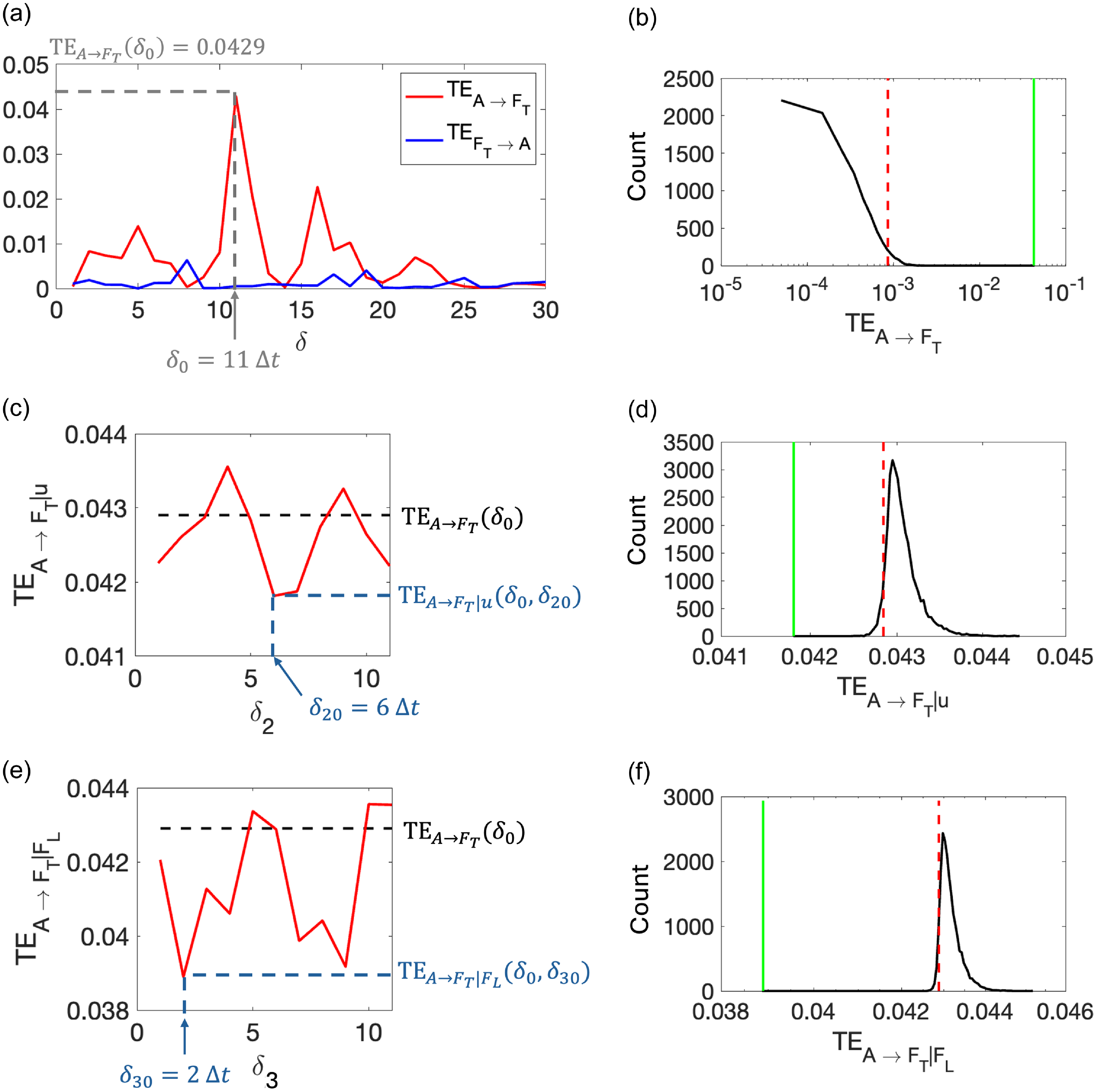
Figure 6. Analysis of experiments with hydrodynamic and electromechanical interaction: (a) transfer entropy from airfoil to trailing rib of the flag ( $\mathrm{TE}_{A \rightarrow F_T}$
) and from flag to airfoil (
$\mathrm{TE}_{A \rightarrow F_T}$
) and from flag to airfoil ( $\mathrm{TE}_{F_T \rightarrow A}$
) for different delays
$\mathrm{TE}_{F_T \rightarrow A}$
) for different delays $\delta$
between
$\delta$
between $A$
and
$A$
and $F_T$
. Peak
$F_T$
. Peak $\mathrm{TE}_{A \rightarrow F_T}$
is observed at a delay of
$\mathrm{TE}_{A \rightarrow F_T}$
is observed at a delay of $\delta _0=11\Delta t$
. At delay
$\delta _0=11\Delta t$
. At delay $\delta _0$
, (c) conditional transfer entropy from airfoil to flag conditioned on streamwise flow speed,
$\delta _0$
, (c) conditional transfer entropy from airfoil to flag conditioned on streamwise flow speed, $\mathrm{TE}_{A \rightarrow F_T| u}(\delta _0,\delta _2)$
, as a function of time delay
$\mathrm{TE}_{A \rightarrow F_T| u}(\delta _0,\delta _2)$
, as a function of time delay $\delta _2$
between
$\delta _2$
between $u$
and
$u$
and $F_T$
(minimum
$F_T$
(minimum $\mathrm{TE}_{A \rightarrow F_T| u}$
is observed at delay
$\mathrm{TE}_{A \rightarrow F_T| u}$
is observed at delay $\delta _{20}=6\Delta t$
) and (e) conditional transfer entropy from airfoil to flag conditioned on flag’s leading rib deflection (
$\delta _{20}=6\Delta t$
) and (e) conditional transfer entropy from airfoil to flag conditioned on flag’s leading rib deflection ( $\mathrm{TE}_{A \rightarrow F_T| F_L}(\delta _0,\delta _3)$
) as a function of time delay
$\mathrm{TE}_{A \rightarrow F_T| F_L}(\delta _0,\delta _3)$
) as a function of time delay $\delta _3$
between
$\delta _3$
between $F_L$
and
$F_L$
and $F_T$
(minimum
$F_T$
(minimum $\mathrm{TE}_{A \rightarrow F_T| F_L}$
is observed at delay
$\mathrm{TE}_{A \rightarrow F_T| F_L}$
is observed at delay $\delta _{20}=2\Delta t$
). Statistical tests: (b)
$\delta _{20}=2\Delta t$
). Statistical tests: (b) $\mathrm{TE}_{A \rightarrow F_T}(\delta _0)$
with respect to its surrogate distribution, (d)
$\mathrm{TE}_{A \rightarrow F_T}(\delta _0)$
with respect to its surrogate distribution, (d) $\mathrm{TE}_{A \rightarrow F_T| u}(\delta _0,\delta _{20})$
with respect to its surrogate distribution and (f)
$\mathrm{TE}_{A \rightarrow F_T| u}(\delta _0,\delta _{20})$
with respect to its surrogate distribution and (f) $\mathrm{TE}_{A \rightarrow F_T| F_L}(\delta _0,\delta _{30})$
with respect to its surrogate distribution. In (b), (d) and (f), green solid lines represent
$\mathrm{TE}_{A \rightarrow F_T| F_L}(\delta _0,\delta _{30})$
with respect to its surrogate distribution. In (b), (d) and (f), green solid lines represent $\mathrm{TE}_{A \rightarrow F_T}(\delta _0)$
,
$\mathrm{TE}_{A \rightarrow F_T}(\delta _0)$
, $\mathrm{TE}_{A \rightarrow F_T| u}(\delta _0,\delta _{20})$
and
$\mathrm{TE}_{A \rightarrow F_T| u}(\delta _0,\delta _{20})$
and $\mathrm{TE}_{A \rightarrow F_T| F_L}(\delta _0,\delta _{30})$
, black solid lines represent their surrogate distributions and red dashed lines mark the
$\mathrm{TE}_{A \rightarrow F_T| F_L}(\delta _0,\delta _{30})$
, black solid lines represent their surrogate distributions and red dashed lines mark the $95$
(or
$95$
(or $5$
) percentile cutoff of the surrogate distributions.
$5$
) percentile cutoff of the surrogate distributions.
Since the airfoil interacts with the flag through the flow, we condition the transfer entropy on the instantaneous flow-speed information encoded in the symbolised time series $\pi _u$
. The conditional transfer entropy from airfoil to flag’s trailing rib, conditioned on flow speed at an intermediate point,
$\pi _u$
. The conditional transfer entropy from airfoil to flag’s trailing rib, conditioned on flow speed at an intermediate point, $\mathrm{TE}_{A \rightarrow F_T|u}(\delta _0,\delta _2)$
, is plotted as a function of the time delay (
$\mathrm{TE}_{A \rightarrow F_T|u}(\delta _0,\delta _2)$
, is plotted as a function of the time delay ( $\delta _2$
) between the flow speed and the flag’s tip deflection in Figure 5c. The figure illustrates that transfer entropy can decrease or increase upon conditioning, depending on the time lag between
$\delta _2$
) between the flow speed and the flag’s tip deflection in Figure 5c. The figure illustrates that transfer entropy can decrease or increase upon conditioning, depending on the time lag between $u$
and
$u$
and $F_T$
. The conditional transfer entropy is minimum at
$F_T$
. The conditional transfer entropy is minimum at $\delta _2=\delta _{20}=6\Delta t=0.2 \; \mathrm{s}$
, suggesting that
$\delta _2=\delta _{20}=6\Delta t=0.2 \; \mathrm{s}$
, suggesting that $u$
can help predict the behaviour of
$u$
can help predict the behaviour of $F_T$
,
$F_T$
, $0.2 \; \mathrm{s}$
ahead of time, due to the existence of the hydrodynamic pathway of interaction. This delay is close to our estimated time lag of
$0.2 \; \mathrm{s}$
ahead of time, due to the existence of the hydrodynamic pathway of interaction. This delay is close to our estimated time lag of $0.23 \; \mathrm{s}$
, between the location of LDV measurement (
$0.23 \; \mathrm{s}$
, between the location of LDV measurement ( $u$
) and the tip of the flag (
$u$
) and the tip of the flag ( $F_T$
) based on the centreline flow speed and the distance along the centreline.
$F_T$
) based on the centreline flow speed and the distance along the centreline.
The significance of the conditional transfer entropy with respect to a surrogate distribution obtained by shuffling the symbolised time series $\pi _u$
is tested in Figure 5d. As described in § 2.4, such a surrogate distribution of the time series breaks the link with
$\pi _u$
is tested in Figure 5d. As described in § 2.4, such a surrogate distribution of the time series breaks the link with $u$
, keeping the
$u$
, keeping the $A$
-
$A$
- $F_T$
dynamics intact. The value of
$F_T$
dynamics intact. The value of $\mathrm{TE}_{A \rightarrow F_T|u}(\delta _0,\delta _{20})$
is found to be significantly reduced (
$\mathrm{TE}_{A \rightarrow F_T|u}(\delta _0,\delta _{20})$
is found to be significantly reduced ( $p=0.0001$
), demonstrating that conditioning on the LDV-recorded flow information significantly reduces the transfer entropy from the upstream airfoil to the downstream flag. This finding suggests that fluid flow is a primary information pathway in the airfoil–flag interaction.
$p=0.0001$
), demonstrating that conditioning on the LDV-recorded flow information significantly reduces the transfer entropy from the upstream airfoil to the downstream flag. This finding suggests that fluid flow is a primary information pathway in the airfoil–flag interaction.
3.3. Hydrodynamic and electromechanical interactions
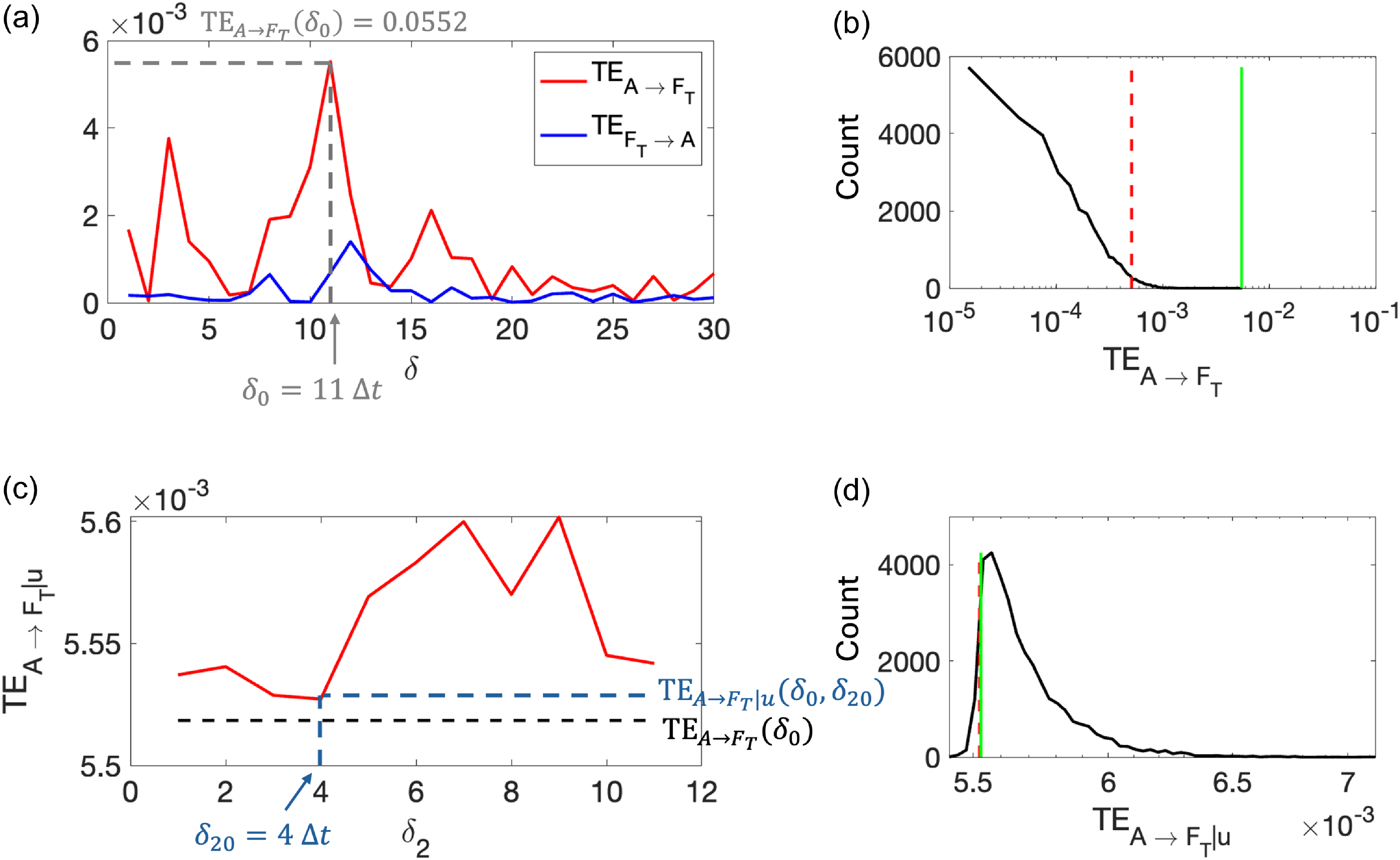
Figure 7. Analysis of experiments with only electromechanical interaction: (a) transfer entropy from airfoil to trailing rib of the flag ( $\mathrm{TE}_{A \rightarrow F_T}$
) and from flag to airfoil (
$\mathrm{TE}_{A \rightarrow F_T}$
) and from flag to airfoil ( $\mathrm{TE}_{F_T \rightarrow A}$
) for different delays
$\mathrm{TE}_{F_T \rightarrow A}$
) for different delays $\delta$
between
$\delta$
between $A$
and
$A$
and $F_T$
. Peak
$F_T$
. Peak $\mathrm{TE}_{A \rightarrow F_T}$
is observed at a delay of
$\mathrm{TE}_{A \rightarrow F_T}$
is observed at a delay of $\delta _0=11\Delta t$
. At delay
$\delta _0=11\Delta t$
. At delay $\delta _0$
, (c) conditional transfer entropy from airfoil to flag conditioned on streamwise flow speed,
$\delta _0$
, (c) conditional transfer entropy from airfoil to flag conditioned on streamwise flow speed, $\mathrm{TE}_{A \rightarrow F_T| u}(\delta _0,\delta _2)$
, as a function of timedelay (
$\mathrm{TE}_{A \rightarrow F_T| u}(\delta _0,\delta _2)$
, as a function of timedelay ( $\delta _2$
) between
$\delta _2$
) between $u$
and
$u$
and $F_T$
. Minimum
$F_T$
. Minimum $\mathrm{TE}_{A \rightarrow F_T| u}$
is observed at delay
$\mathrm{TE}_{A \rightarrow F_T| u}$
is observed at delay $\delta _{20}=4\Delta t$
. Statistical tests: (b)
$\delta _{20}=4\Delta t$
. Statistical tests: (b) $\mathrm{TE}_{A \rightarrow F_T}(\delta _0)$
with respect to its surrogate distribution and (d)
$\mathrm{TE}_{A \rightarrow F_T}(\delta _0)$
with respect to its surrogate distribution and (d) $\mathrm{TE}_{A \rightarrow F_T| u}(\delta _0,\delta _{20})$
with respect to its surrogate distribution. In (b) and (d), green solid lines represent
$\mathrm{TE}_{A \rightarrow F_T| u}(\delta _0,\delta _{20})$
with respect to its surrogate distribution. In (b) and (d), green solid lines represent $\mathrm{TE}_{A \rightarrow F_T}(\delta _0)$
and
$\mathrm{TE}_{A \rightarrow F_T}(\delta _0)$
and $\mathrm{TE}_{A \rightarrow F_T| u}(\delta _0,\delta _{20})$
, black solid lines represent their surrogate distributions and red dashed lines mark the
$\mathrm{TE}_{A \rightarrow F_T| u}(\delta _0,\delta _{20})$
, black solid lines represent their surrogate distributions and red dashed lines mark the $95$
(or
$95$
(or $5$
) percentile cutoff of the surrogate distributions.
$5$
) percentile cutoff of the surrogate distributions.
Second, we study the experimental case in which both airfoil and flag are actively controlled in the presence of a steady flow. The actuation of the flag’s leading rib follows that of the airfoil with a time delay and added random noise. In this scenario, there are two major pathways of interaction between the airfoil and the flag – hydrodynamic and electromechanical. Figure 6a shows the variation of transfer entropies, $\mathrm{TE}_{A \rightarrow F_T}$
and
$\mathrm{TE}_{A \rightarrow F_T}$
and $\mathrm{TE}_{F_T \rightarrow A}$
, with the time delay between the airfoil and the flag’s trailing rib (
$\mathrm{TE}_{F_T \rightarrow A}$
, with the time delay between the airfoil and the flag’s trailing rib ( $\delta$
). Similar to the previous case,
$\delta$
). Similar to the previous case, $\mathrm{TE}_{A \rightarrow F_T}\gt \mathrm{TE}_{F_T \rightarrow A}$
for most
$\mathrm{TE}_{A \rightarrow F_T}\gt \mathrm{TE}_{F_T \rightarrow A}$
for most $\delta$
values, suggesting a stronger influence of the airfoil on the flag than vice versa. The peak
$\delta$
values, suggesting a stronger influence of the airfoil on the flag than vice versa. The peak $\mathrm{TE}_{A \rightarrow F_T}$
occurs at
$\mathrm{TE}_{A \rightarrow F_T}$
occurs at $\delta _0=11 \Delta t = 0.37 \; \mathrm{s}$
, which is greater than the time delay of interaction identified in the presence of the hydrodynamic pathway alone in the previous case (
$\delta _0=11 \Delta t = 0.37 \; \mathrm{s}$
, which is greater than the time delay of interaction identified in the presence of the hydrodynamic pathway alone in the previous case ( $\delta _0=0.3 \; \mathrm{s}$
). This indicates that the combined presence of the electromechanical interaction in addition to the hydrodynamic interaction increases the effective time lag of the causal influence of the airfoil’s motion on the flag’s tip to
$\delta _0=0.3 \; \mathrm{s}$
). This indicates that the combined presence of the electromechanical interaction in addition to the hydrodynamic interaction increases the effective time lag of the causal influence of the airfoil’s motion on the flag’s tip to $0.37 \; \mathrm{s}$
. Such a finding is reasonable since the flag’s leading rib is actuated with a delay of
$0.37 \; \mathrm{s}$
. Such a finding is reasonable since the flag’s leading rib is actuated with a delay of $0.3 \; \mathrm{s}$
with respect to the airfoil and the transmission of the deflection from the leading rib of the flag to its trailing rib takes additional time. Therefore, the overall time delay in this experimental case is expected to be greater than the previous one. Further, the peak transfer entropy
$0.3 \; \mathrm{s}$
with respect to the airfoil and the transmission of the deflection from the leading rib of the flag to its trailing rib takes additional time. Therefore, the overall time delay in this experimental case is expected to be greater than the previous one. Further, the peak transfer entropy $\mathrm{TE}_{A \rightarrow F_T}(\delta _0)$
is statistically significant (Figure 6b), illustrating that in this experimental case as well, the airfoil has an overall causal influence on the flag.
$\mathrm{TE}_{A \rightarrow F_T}(\delta _0)$
is statistically significant (Figure 6b), illustrating that in this experimental case as well, the airfoil has an overall causal influence on the flag.
In this experimental condition, the airfoil interacts with the flag via two distinct pathways – hydrodynamic and electromechanical. The LDV-measured speed $u$
encodes part of the flow information while the deflection of the flag’s leading rib
$u$
encodes part of the flow information while the deflection of the flag’s leading rib $F_L$
encodes the electromechanical information. First, we study the conditional transfer entropy conditioned on
$F_L$
encodes the electromechanical information. First, we study the conditional transfer entropy conditioned on $u$
,
$u$
, $\mathrm{TE}_{A \rightarrow F_T|u}$
, at a fixed
$\mathrm{TE}_{A \rightarrow F_T|u}$
, at a fixed $F_T$
-
$F_T$
- $A$
time delay (
$A$
time delay ( $\delta =\delta _0$
) and for different time lags (
$\delta =\delta _0$
) and for different time lags ( $\delta _2$
) between
$\delta _2$
) between $F_T$
and
$F_T$
and $u$
, as illustrated in Figure 6c. It is evident that conditioning on
$u$
, as illustrated in Figure 6c. It is evident that conditioning on $u$
is most effective in reducing the transfer entropy at a time delay of
$u$
is most effective in reducing the transfer entropy at a time delay of $\delta _{20}=6 \Delta t=0.2 \; \mathrm{s}$
. This is identical to the time delay observed by transfer entropy analysis in the absence of the mechanical coupling, which one would expect since the hydrodynamic coupling is independent of the electromechanical coupling. Compared with the surrogate distribution with shuffled
$\delta _{20}=6 \Delta t=0.2 \; \mathrm{s}$
. This is identical to the time delay observed by transfer entropy analysis in the absence of the mechanical coupling, which one would expect since the hydrodynamic coupling is independent of the electromechanical coupling. Compared with the surrogate distribution with shuffled $u$
time series in Figure 6d, the conditional transfer entropy
$u$
time series in Figure 6d, the conditional transfer entropy $\mathrm{TE}_{A \rightarrow F_T|u}(\delta _0,\delta _{20})$
value is significantly less (
$\mathrm{TE}_{A \rightarrow F_T|u}(\delta _0,\delta _{20})$
value is significantly less ( $p=0.0001$
). Even in the presence of other pathways of interaction, conditioning on the flow-speed information successfully reduces the transfer entropy from airfoil to flag, compared with conditioning it on a randomly shuffled time series. This suggests that the causal influence of airfoil on flag significantly reduces with the knowledge of the flow speed.
$p=0.0001$
). Even in the presence of other pathways of interaction, conditioning on the flow-speed information successfully reduces the transfer entropy from airfoil to flag, compared with conditioning it on a randomly shuffled time series. This suggests that the causal influence of airfoil on flag significantly reduces with the knowledge of the flow speed.
Next, we analyse conditional transfer entropy conditioned on $F_L$
,
$F_L$
, $\mathrm{TE}_{A \rightarrow F_T|F_L}$
, at a fixed
$\mathrm{TE}_{A \rightarrow F_T|F_L}$
, at a fixed $F_T$
-
$F_T$
- $A$
time delay (
$A$
time delay ( $\delta =\delta _0$
) and for different time delays (
$\delta =\delta _0$
) and for different time delays ( $\delta _3$
) between
$\delta _3$
) between $F_T$
and
$F_T$
and $F_L$
, in Figure 6e. The
$F_L$
, in Figure 6e. The $F_L$
-conditioning reduces transfer entropy from the airfoil to the flag’s tip the most at a time lag of
$F_L$
-conditioning reduces transfer entropy from the airfoil to the flag’s tip the most at a time lag of $\delta _{30}=2 \Delta t=0.07 \; \mathrm{s}$
. This indicates that the time required for the deflection at the leading rib of the flag to propagate to its trailing rib is
$\delta _{30}=2 \Delta t=0.07 \; \mathrm{s}$
. This indicates that the time required for the deflection at the leading rib of the flag to propagate to its trailing rib is $\approx 0.07 \; \mathrm{s}$
. The secondary minima at a time lag of
$\approx 0.07 \; \mathrm{s}$
. The secondary minima at a time lag of $\delta _{30}=9 \Delta t=0.3 \;\mathrm{s}$
indicates the presence of multi-time-scale information flow through the length of the slender flag from the leading rib to the trailing rib. Additionally, Figure 6f demonstrates that conditional transfer entropy is significantly less than the null distribution with a p-value of
$\delta _{30}=9 \Delta t=0.3 \;\mathrm{s}$
indicates the presence of multi-time-scale information flow through the length of the slender flag from the leading rib to the trailing rib. Additionally, Figure 6f demonstrates that conditional transfer entropy is significantly less than the null distribution with a p-value of $p=0.0001$
. Therefore, conditioning on the mechanical coupling information significantly reduces the transfer entropy, as compared with conditioning the same on a randomly shuffled timeseries. This indicates that the overall causal influence of the airfoil on the flag significantly decreases on account of the knowledge of the motion of the flag’s leading rib.
$p=0.0001$
. Therefore, conditioning on the mechanical coupling information significantly reduces the transfer entropy, as compared with conditioning the same on a randomly shuffled timeseries. This indicates that the overall causal influence of the airfoil on the flag significantly decreases on account of the knowledge of the motion of the flag’s leading rib.
3.4. Electromechanical interaction
In the third case, the experiments were conducted in the absence of a flow, which implies that the airfoil and the flag primarily interact via electromechanical coupling only without any hydrodynamic interaction. As illustrated in Figures 7a and 7b, the transfer entropy analysis shows a significant influence of the airfoil’s motion on the flag’s tip deflection at a time delay of $\delta _0=11 \Delta t = 0.37 \; \mathrm{s}$
. However, upon conditioning on
$\delta _0=11 \Delta t = 0.37 \; \mathrm{s}$
. However, upon conditioning on $u$
, conditional transfer entropy is greater than transfer entropy value for all time delays
$u$
, conditional transfer entropy is greater than transfer entropy value for all time delays $\delta _2$
, as shown in Figure 7c. In addition, the minimum conditional transfer entropy,
$\delta _2$
, as shown in Figure 7c. In addition, the minimum conditional transfer entropy, $\mathrm{TE}_{A \rightarrow F_T | u} (\delta _0,\delta _{20})$
, is not significantly (
$\mathrm{TE}_{A \rightarrow F_T | u} (\delta _0,\delta _{20})$
, is not significantly ( $p=0.07$
) smaller than transfer entropy conditioned on a randomly shuffled time series (Figure 7d). We can infer that conditioning on flow information only reduces transfer entropy from airfoil to flag if a hydrodynamic interaction is present. Therefore, such a conditional transfer entropy can be used to test the presence or absence of hydrodynamic interaction pathway in an unknown case.
$p=0.07$
) smaller than transfer entropy conditioned on a randomly shuffled time series (Figure 7d). We can infer that conditioning on flow information only reduces transfer entropy from airfoil to flag if a hydrodynamic interaction is present. Therefore, such a conditional transfer entropy can be used to test the presence or absence of hydrodynamic interaction pathway in an unknown case.
4. Discussion and conclusions
A controlled robotic set-up in a water channel was designed to recreate a simplified fish schooling subsystem. Experiments were conducted using an upstream pitching airfoil and a downstream flapping flag representing two fish swimming inline. The airfoil’s motion influenced the flag’s behaviour via two independent pathways – hydrodynamic and eletromechanical. The hydrodynamic coupling was constituted by vortex-induced pressure variations generated by the pitching of the upstream airfoil that causes the compliant flag downstream to flap in response. Further, the leading rib of the flag was actuated to follow the motion of the airfoil with a delay, therefore causing the flag to flap in response to the electromechanical coupling. Experiments were conducted under three conditions – (i) with only hydrodynamic coupling, (ii) with hydrodynamic and electromechanical coupling and (iii) with only electromechanical coupling. Besides monitoring the movements of both the airfoil and the flag, the LDV technique was employed to measure the streamwise flow speed at a midpoint. This data served as a source of information on the hydrodynamic interaction pathway between the airfoil and the flag.
The information-theoretic analysis was conducted using properly conditioned experimental data of the airfoil, flag and flow speed. It was demonstrated that transfer entropy from the airfoil to the flag can recognise and quantify the causal influence of the airfoil on the flag under all three experimental conditions. In addition, the method identifies the appropriate time delay of the interaction with reasonable accuracy. Our findings suggest that transfer entropy can be adapted to identify causal influence between units of a system that are interacting via single or multiple pathways.
By conditioning on a measurable physical quantity related to one pathway, that is, flow-speed information related to hydrodynamic coupling, one can reduce transfer entropy from the airfoil to the flag significantly. This conditional transfer entropy is competent in reducing the information flow from the airfoil to the flag on account of knowledge about the flow, if the hydrodynamic interaction exists. Similarly, conditioning on information related to the electromechanical coupling (undulation of the flag’s leading rib) reduces the transfer entropy from the airfoil to the flag, only if the electromechanical coupling is present. This implies that conditional transfer entropy based on measured experimental data related to one particular interaction pathway helps disentangle the other pathways from this one.
The current study employs an experimental set-up with unidirectional interactions only, from the airfoil to the flag. In future work, transfer entropy based method will be formulated for similar systems to disentangle bidirectional interactions. While the present work demonstrates the ability of conditional transfer entropy in accounting for the contributions of different interaction pathways, it does not precisely quantify the contributions of each pathway of interaction. Overall, the study suggests that conditioning transfer entropy on experimentally measured relevant information, one can identify unknown interactions between different components of a fluid–structure interaction system and estimate the associated time lags of the processes of the system. In the future, this mechanism will be extended to distinguish the contributions of various interaction pathways within biological complex systems, such as fish schools. Our approach is expected to apply directly to spatially disperse schools where fish are far apart, so that one may hypothesise weak coupling between the units of the complex system (Porfiri & Marín, Reference Porfiri and Marín2017, Reference Porfiri and Marín2018). Prudence is warranted when dealing with dense schools for which the direct application of transfer entropy may lead to false inferences due to common driver and chain effects. Addressing these issues may require the use of causation entropy (Sun & Bollt, Reference Sun and Bollt2014; Sun et al. Reference Sun, Taylor and Bollt2015) or the inclusion of coarse observables for the entire school (Wang et al. Reference Wang, Miller, Lizier, Prokopenko, Rossi and de Polavieja2012).
Acknowledgements
The authors would like to thank Ms A. Ravindran for her help during the experimentation.
Funding
The research was supported by the National Science Foundation under Grant No. CMMI-1901697. R.D. would also like to acknowledge Indian Institute of Science for the Startup Research Grant.
Competing interests
The authors declare no conflict of interest.
Ethical standards
The research meets all ethical guidelines, including adherence to the legal requirements of the study country.


 Open access