


Impact Statement
Roughness, such as biofouling on ship hulls, significantly increases vehicle drag, leading to higher fuel consumption and operational costs. Accurate prediction methods for skin friction drag caused by rough surfaces are essential for improving vehicle performance and reducing expenses. However, a challenge remains on how to assign a representative quantity to describe flow over heterogeneous surfaces while maintaining the functional relationships between drag and roughness scales. This study compares three averaging methods – arithmetic average and unweighted and weighted power means – for estimating the equivalent sandgrain roughness ( $k_s$
) over streamwise-heterogeneous surfaces with
$k_s$
) over streamwise-heterogeneous surfaces with $\beta$
, uniform or Gaussian topographical distributions. Results show that the weighted power mean outperformed the other methods, especially for
$\beta$
, uniform or Gaussian topographical distributions. Results show that the weighted power mean outperformed the other methods, especially for $\beta$
distributions, reducing error between effective and estimated drag parameters to less than
$\beta$
distributions, reducing error between effective and estimated drag parameters to less than $2.6\,\%$
. The weighted method also excelled at higher Reynolds numbers, making it the most accurate for predicting drag over heterogeneous surfaces, with practical benefits for assessing biofouling impacts on marine vehicles.
$2.6\,\%$
. The weighted method also excelled at higher Reynolds numbers, making it the most accurate for predicting drag over heterogeneous surfaces, with practical benefits for assessing biofouling impacts on marine vehicles.
1. Introduction
The economic and vehicle performance impacts of frictional drag are significantly exacerbated in the presence of roughness (Kempf Reference Kempf1937; Schultz et al. Reference Schultz, Bendick, Holm and Hertel2011; Schultz Reference Schultz2007). For instance, biofouling roughness, commonly observed in marine and naval applications, is regarded as one of the largest contributors to fuel consumption costs. For a single, mid-sized US Arleigh Burke destroyer DDG-51, the typical fouling conditions of just heavy slime generate a 10.3 % increase in fuel consumption compared with a hydraulically smooth hull. This translates to additional yearly fuel costs of $1.15 million per ship, aside from the significant expenses and mission interruptions due to dry-dock and hull-cleaning schedules Schultz et al. (Reference Schultz, Bendick, Holm and Hertel2011). Drag prediction capabilities based on fouling conditions will help mitigate these expenses of additional fuel and inefficiently scheduled anti-fouling measures, but current decision-making methods based on visual inspections of the hull need significant improvement. It is difficult to ascribe a single length-scale quantity or parameter from a physical inspection of the surface to describe the overall ship hull due to the complexity of geometric roughness parameters, including roughness height, frontal and planform solidity, skewness and element directionality, amongst others (Chung et al. Reference Chung, Hutchins, Schultz and Flack2021). For this reason, rough surfaces are often described in terms of a hydrodynamic quantity, the equivalent sandgrain roughness parameter, $k_{s}$
, which equates to a height of uniform sandgrain roughness that would result in the same skin friction drag as the surface of interest in a fully rough regime (Jiménez Reference Jiménez2004).
$k_{s}$
, which equates to a height of uniform sandgrain roughness that would result in the same skin friction drag as the surface of interest in a fully rough regime (Jiménez Reference Jiménez2004).
Since the $k_s$
parameter is closely related to the skin friction drag over a rough surface, it is used in combination with the integral formulation of turbulent boundary layers to make full-scale predictions of the impact of surface roughness on vehicle performance deficiencies (Monty et al. Reference Monty, Dogan, Hanson, Scardino, Ganapathisubramani and Hutchins2016; Schultz Reference Schultz2007). This process involves an assumption of a mean velocity profile, wake function and strength, which for a flat plate (often used as a simple representation of a ship hull) can be further simplified such that the boundary-layer growth and related frictional quantities are dependent on only the streamwise development and vehicle operating conditions (i.e. speed and fluid viscosity) (Chung et al. Reference Chung, Hutchins, Schultz and Flack2021). There are many approaches to characterise the development of the momentum integral equations, notably by Granville (Reference Granville1958), Monty et al. (Reference Monty, Dogan, Hanson, Scardino, Ganapathisubramani and Hutchins2016), Prandtl & Schlichting (Reference Prandtl and Schlichting1934) and Pullin et al. (Reference Pullin, Hutchins and Chung2017), which can be modified to account for surface heterogeneity (see § 2.3). Other prediction methods such as that by Song et al. (Reference Song, Kim, Demirel and Yang2023) are shown to be effective in estimating the heterogeneous surface resistance, but require knowledge of key input parameters such as the roughness impact factor which has yet to be generalised for universal operating conditions. When related to the roughness function
$k_s$
parameter is closely related to the skin friction drag over a rough surface, it is used in combination with the integral formulation of turbulent boundary layers to make full-scale predictions of the impact of surface roughness on vehicle performance deficiencies (Monty et al. Reference Monty, Dogan, Hanson, Scardino, Ganapathisubramani and Hutchins2016; Schultz Reference Schultz2007). This process involves an assumption of a mean velocity profile, wake function and strength, which for a flat plate (often used as a simple representation of a ship hull) can be further simplified such that the boundary-layer growth and related frictional quantities are dependent on only the streamwise development and vehicle operating conditions (i.e. speed and fluid viscosity) (Chung et al. Reference Chung, Hutchins, Schultz and Flack2021). There are many approaches to characterise the development of the momentum integral equations, notably by Granville (Reference Granville1958), Monty et al. (Reference Monty, Dogan, Hanson, Scardino, Ganapathisubramani and Hutchins2016), Prandtl & Schlichting (Reference Prandtl and Schlichting1934) and Pullin et al. (Reference Pullin, Hutchins and Chung2017), which can be modified to account for surface heterogeneity (see § 2.3). Other prediction methods such as that by Song et al. (Reference Song, Kim, Demirel and Yang2023) are shown to be effective in estimating the heterogeneous surface resistance, but require knowledge of key input parameters such as the roughness impact factor which has yet to be generalised for universal operating conditions. When related to the roughness function $\Delta U^+$
, the
$\Delta U^+$
, the $k_s$
parameter can also describe the downward shift of the viscous-scaled mean velocity profile using the expression
$k_s$
parameter can also describe the downward shift of the viscous-scaled mean velocity profile using the expression $\Delta U^+ = (1/\kappa )\log _{\rm e}(k_s^+) + A - B$
, where
$\Delta U^+ = (1/\kappa )\log _{\rm e}(k_s^+) + A - B$
, where $\kappa$
,
$\kappa$
, $A$
and
$A$
and $B$
are empirical constants, assumed to be approximately
$B$
are empirical constants, assumed to be approximately $\kappa = 0.4$
(i.e. the von Kármán constant),
$\kappa = 0.4$
(i.e. the von Kármán constant), $A = 5$
and
$A = 5$
and $B = 8.5$
. The superscript ‘
$B = 8.5$
. The superscript ‘ $+$
’ implies normalisation on viscous coordinates by the shear velocity,
$+$
’ implies normalisation on viscous coordinates by the shear velocity, $u_\tau$
, and the kinematic viscosity,
$u_\tau$
, and the kinematic viscosity, $\nu$
.
$\nu$
.
For heterogeneous roughness, there is the added complication of how to assign a single $k_s$
value to a surface characterised by non-functional and random variations of the roughness topography that may result in variations of the local statistical properties within a length range of the order of the outer layer length scales (Chung et al. Reference Chung, Hutchins, Schultz and Flack2021). In the case of ship biofouling, which is inherently patchy in distribution, the current method to assign a representative value involves taking an arithmetic average of discrete
$k_s$
value to a surface characterised by non-functional and random variations of the roughness topography that may result in variations of the local statistical properties within a length range of the order of the outer layer length scales (Chung et al. Reference Chung, Hutchins, Schultz and Flack2021). In the case of ship biofouling, which is inherently patchy in distribution, the current method to assign a representative value involves taking an arithmetic average of discrete $k_s$
values corresponding to a range of roughness heights across subjectively selected observations of a ship hull (O’Leary & Anderson Reference O’Leary and Anderson2003; Naval Sea Systems Command 2006).
$k_s$
values corresponding to a range of roughness heights across subjectively selected observations of a ship hull (O’Leary & Anderson Reference O’Leary and Anderson2003; Naval Sea Systems Command 2006).
In a study of equivalent parameters for spanwise-heterogeneous roughness, Hutchins et al. (Reference Hutchins, Ganapathisubramani, Schultz and Pullin2023) described the flaws of this arithmetic averaging method, as it incorrectly assumes a linear relation between $k_s$
and the integrated skin friction drag
$k_s$
and the integrated skin friction drag $C_F$
. Given an appropriate empirical fit of the two variables, Hutchins et al. (Reference Hutchins, Ganapathisubramani, Schultz and Pullin2023) suggested an alternative averaging method using the power mean. This method was tested on many roughness iterations of a theoretical flat plate sectioned into equally spaced areas of varying spanwise
$C_F$
. Given an appropriate empirical fit of the two variables, Hutchins et al. (Reference Hutchins, Ganapathisubramani, Schultz and Pullin2023) suggested an alternative averaging method using the power mean. This method was tested on many roughness iterations of a theoretical flat plate sectioned into equally spaced areas of varying spanwise $k_s$
that followed either a
$k_s$
that followed either a $\beta$
or uniform probability density distribution. The study found that the equivalent sandgrain roughness parameter computed from the power mean,
$\beta$
or uniform probability density distribution. The study found that the equivalent sandgrain roughness parameter computed from the power mean, $k_{s_{eq}}$
, resulted in a less than 1 % error in the skin friction drag estimates compared with a direct calculation of
$k_{s_{eq}}$
, resulted in a less than 1 % error in the skin friction drag estimates compared with a direct calculation of $C_F$
determined from the momentum integral method (Hutchins et al. Reference Hutchins, Ganapathisubramani, Schultz and Pullin2023).
$C_F$
determined from the momentum integral method (Hutchins et al. Reference Hutchins, Ganapathisubramani, Schultz and Pullin2023).
Streamwise heterogeneity is also widely observed in biofouling conditions. The flow over the heterogeneous surface can be microscopically treated as randomised smooth-to-rough and rough-to-smooth transitions. In the presence of such perturbations, the flow generates internal boundary layers that may take up to 10δ–20 $\delta$
to recover (Antonia & Luxton Reference Antonia and Luxton1972; Li et al. Reference Li, de Silva, Rouhi, Baidya, Chung, Marusic and Hutchins2019). Predicting the evolution of the flow conditions due to the individual offshoots is not as useful as an average representative condition of the entire surface. Although the local skin friction rises and falls in response to the perturbations of the surface conditions, there is a tendency for the friction to relax towards the equilibrium condition after sufficient streamwise distance (Andreopoulos & Wood Reference Andreopoulos and Wood1982). Suastika et al. (Reference Suastika, Hakim, Nugroho, Nasirudin, Utama, Monty and Ganapathisubramani2021) also found that the integrated drag over a heterogeneous roughness patch was very similar to that over a homogeneous rough surface of the same extent, assuming the same boundary conditions are applied. For a flat plate with a zero pressure gradient, the integrated skin friction drag,
$\delta$
to recover (Antonia & Luxton Reference Antonia and Luxton1972; Li et al. Reference Li, de Silva, Rouhi, Baidya, Chung, Marusic and Hutchins2019). Predicting the evolution of the flow conditions due to the individual offshoots is not as useful as an average representative condition of the entire surface. Although the local skin friction rises and falls in response to the perturbations of the surface conditions, there is a tendency for the friction to relax towards the equilibrium condition after sufficient streamwise distance (Andreopoulos & Wood Reference Andreopoulos and Wood1982). Suastika et al. (Reference Suastika, Hakim, Nugroho, Nasirudin, Utama, Monty and Ganapathisubramani2021) also found that the integrated drag over a heterogeneous roughness patch was very similar to that over a homogeneous rough surface of the same extent, assuming the same boundary conditions are applied. For a flat plate with a zero pressure gradient, the integrated skin friction drag, $C_F$
, is approximately inversely proportional to the streamwise Reynolds number,
$C_F$
, is approximately inversely proportional to the streamwise Reynolds number, $Re_x$
(Monty et al. Reference Monty, Dogan, Hanson, Scardino, Ganapathisubramani and Hutchins2016). Consequently, despite roughness-induced local variations in skin friction, the frictional drag tends to be most significant near the leading edge of the plate and diminishes as the Reynolds number increases, and an equilibrium assumption can be expected to produce viable results.
$Re_x$
(Monty et al. Reference Monty, Dogan, Hanson, Scardino, Ganapathisubramani and Hutchins2016). Consequently, despite roughness-induced local variations in skin friction, the frictional drag tends to be most significant near the leading edge of the plate and diminishes as the Reynolds number increases, and an equilibrium assumption can be expected to produce viable results.
For a streamwise-varying surface, the significance of the initial conditions can be accounted for by implementing a weighting scheme with the power mean. This investigation aims to extend the work of Hutchins et al. (Reference Hutchins, Ganapathisubramani, Schultz and Pullin2023) by comparing the validity of three averaging schemes – arithmetic averaging (AHR), the unweighted power mean (UPM) and the weighted power mean (WPM) – for iterations of streamwise-heterogeneous plates configured with roughness distribution following $\beta$
, uniform or Gaussian functions. The theoretical set-up is similar to that of Hutchins et al. (Reference Hutchins, Ganapathisubramani, Schultz and Pullin2023), but now the roughness plate is sectioned into equally spaced, streamwise-varying, roughness patches which also follow either a
$\beta$
, uniform or Gaussian functions. The theoretical set-up is similar to that of Hutchins et al. (Reference Hutchins, Ganapathisubramani, Schultz and Pullin2023), but now the roughness plate is sectioned into equally spaced, streamwise-varying, roughness patches which also follow either a $\beta$
, uniform or Gaussian distribution. The effective sandgrain roughness parameters computed using the averaging methods (
$\beta$
, uniform or Gaussian distribution. The effective sandgrain roughness parameters computed using the averaging methods ( $k_{s_{eq}}$
) and their corresponding drag values (
$k_{s_{eq}}$
) and their corresponding drag values ( $C_{F_{eq}}$
) are referred to with a subscript ‘eq’. These are compared with ‘true’ values estimated from a modified momentum integral method and are denoted with a subscript ‘eff’ (i.e.
$C_{F_{eq}}$
) are referred to with a subscript ‘eq’. These are compared with ‘true’ values estimated from a modified momentum integral method and are denoted with a subscript ‘eff’ (i.e. $k_{s_{eff}}$
and
$k_{s_{eff}}$
and $C_{F_{eff}}$
).
$C_{F_{eff}}$
).
2. Methodology
2.1. Roughness distribution characteristics
The sandgrain roughness parameter values considered in the analysis ranged from $k_{s_1} = 15$
μm to
$k_{s_1} = 15$
μm to $k_{s_2} = 10$
mm, which encompasses a range of
$k_{s_2} = 10$
mm, which encompasses a range of $k_s$
heights between the hydraulically smooth regime for flow at
$k_s$
heights between the hydraulically smooth regime for flow at $15$
knots and estimates of recorded naval biofouling heights provided by Schultz (Reference Schultz2007). The plate configurations were of length
$15$
knots and estimates of recorded naval biofouling heights provided by Schultz (Reference Schultz2007). The plate configurations were of length $L = 100$
m, divided into ten equal-area sections, unless specified for discussion of Reynolds number effects (for which see § 3.2). To capture the variability of
$L = 100$
m, divided into ten equal-area sections, unless specified for discussion of Reynolds number effects (for which see § 3.2). To capture the variability of $k_s$
across the roughness plates, three distinct distribution types were implemented with probability distributions following
$k_s$
across the roughness plates, three distinct distribution types were implemented with probability distributions following $\beta$
, Gaussian or uniform functions, depicted as histograms in figure 1 for which the probability density functions are provided in table 1. The ten patch sections were each randomly assigned a
$\beta$
, Gaussian or uniform functions, depicted as histograms in figure 1 for which the probability density functions are provided in table 1. The ten patch sections were each randomly assigned a $k_s$
, the effective sandgrain roughness from the distribution under investigation, to produce one iteration of the plate configuration. This process was repeated for 10 000 iterations (per distribution) to obtain statistically converged results.
$k_s$
, the effective sandgrain roughness from the distribution under investigation, to produce one iteration of the plate configuration. This process was repeated for 10 000 iterations (per distribution) to obtain statistically converged results.
Table 1. Probability density functions for the investigated roughness configurations. The effective sandgrain roughness, $k_s$
, for the patch is randomly selected between the lower and upper limits of
$k_s$
, for the patch is randomly selected between the lower and upper limits of $k_{s_1} = 15$ $\mu m$
and
$\mu m$
and $k_{s_2} = 10$
mm, respectively.
$k_{s_2} = 10$
mm, respectively.
Figure 1. Probability density functions of the roughness distributions: $\beta$
(left), uniform (middle) and Gaussian (right).
$\beta$
(left), uniform (middle) and Gaussian (right).
Among the investigated configurations, the $\beta$
distribution emerged as the most relevant for practical field applications. Notably, the
$\beta$
distribution emerged as the most relevant for practical field applications. Notably, the $\beta$
function skews the
$\beta$
function skews the $k_s$
distribution, biasing it towards smaller height values. This characteristic aligns closely with observations in real-world scenarios, where fine-scale roughness elements often dominate the surface profile. While a strict Gaussian distribution is unlikely to be found in biofouling applications, it is an explored function to test the viability of the WPM approach for various surface configurations.
$k_s$
distribution, biasing it towards smaller height values. This characteristic aligns closely with observations in real-world scenarios, where fine-scale roughness elements often dominate the surface profile. While a strict Gaussian distribution is unlikely to be found in biofouling applications, it is an explored function to test the viability of the WPM approach for various surface configurations.
2.2. Streamwise weights for the power mean
A heterogeneous roughness plate of length $L$
is sectioned into
$L$
is sectioned into $N$
patches, each of area
$N$
patches, each of area $A_i$
, where the subscript
$A_i$
, where the subscript $i$
represents the characteristic parameter for each patch (i.e.
$i$
represents the characteristic parameter for each patch (i.e. $i = 1,2,3,\ldots ,N$
). Current practices of estimating an equivalent sandgrain roughness for a heterogeneous surface involve taking the arithmetic mean by the use of the average hull roughness (AHR):
$i = 1,2,3,\ldots ,N$
). Current practices of estimating an equivalent sandgrain roughness for a heterogeneous surface involve taking the arithmetic mean by the use of the average hull roughness (AHR):
 \begin{equation} k_{s_{ahr}} = \frac {1}{A}\sum _{i=1}^{N} A_i k_{s_{i}} .\end{equation}
As the roughness drag, $C_F$
, can be approximately related to
$C_F$
, can be approximately related to $k_s/L$
via a power law, Hutchins et al. (Reference Hutchins, Ganapathisubramani, Schultz and Pullin2023) defined the equivalent homogeneous roughness length via the power mean as
$k_s/L$
via a power law, Hutchins et al. (Reference Hutchins, Ganapathisubramani, Schultz and Pullin2023) defined the equivalent homogeneous roughness length via the power mean as
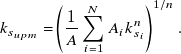 \begin{equation} k_{s_{upm}} = \left (\frac {1}{A}\sum _{i=1}^{N} A_i k_{s_{i}}^n \right )^{1/n} .\end{equation}
An exponent $n = 0.25$
was used as the power operator for the power mean approach. This value was chosen based on the study by Hutchins et al. (Reference Hutchins, Ganapathisubramani, Schultz and Pullin2023) who found that the optimal power operator is one that would reduce the error in the plate integrated drag assuming a homogeneous sandgrain roughness parameter. This study found that variations of
$n = 0.25$
was used as the power operator for the power mean approach. This value was chosen based on the study by Hutchins et al. (Reference Hutchins, Ganapathisubramani, Schultz and Pullin2023) who found that the optimal power operator is one that would reduce the error in the plate integrated drag assuming a homogeneous sandgrain roughness parameter. This study found that variations of $n \pm 0.05$
would still result in more accurate estimates of the drag in comparison with a simple arithmetic average (i.e.
$n \pm 0.05$
would still result in more accurate estimates of the drag in comparison with a simple arithmetic average (i.e. $n = 1$
). When accounting for a streamwise-varying roughness pattern, the expression in (2.2) is slightly modified to include streamwise-dependent weights:
$n = 1$
). When accounting for a streamwise-varying roughness pattern, the expression in (2.2) is slightly modified to include streamwise-dependent weights:
 \begin{equation} k_{s_{wpm}} = \left (\frac {1}{A}\sum _{i=1}^{N} A_i W_{i_{N}} k_{s_{i}}^n \right )^{1/n} .\end{equation}
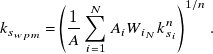
The weighted contribution of each area is denoted as $W_{i_{N}}$
and is determined by considering the drag contribution of each section,
$W_{i_{N}}$
and is determined by considering the drag contribution of each section, $C_{F_{i}}$
as shown in figure 2. Averaging
$C_{F_{i}}$
as shown in figure 2. Averaging $C_{F_{i}}$
over the entire plate results in the overall drag over the full plate length and is defined as
$C_{F_{i}}$
over the entire plate results in the overall drag over the full plate length and is defined as $C_{F_{L}}$
:
$C_{F_{L}}$
:
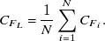 \begin{equation} C_{F_{L}} = \frac {1}{N} \sum _{i=1}^{N} C_{F_{i}} .\end{equation}
The drag $C_{F_{i}}$
over each patch can be iteratively solved for by considering the drag over incrementally increasing lengths of the plate
$C_{F_{i}}$
over each patch can be iteratively solved for by considering the drag over incrementally increasing lengths of the plate $l_i$
in a similarly defined average as
$l_i$
in a similarly defined average as
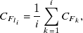 \begin{equation} C_{F_{l_{i}}} = \frac {1}{i} \sum _{k=1}^{i} C_{F_{k}} ,\end{equation}
where the integrated drag of the first patch is equivalent to the drag of the plate of length $l_1$
, i.e.
$l_1$
, i.e. $C_{F_1} = C_{F_{l_1}}$
. The weighting distribution for a plate with
$C_{F_1} = C_{F_{l_1}}$
. The weighting distribution for a plate with $N$
sections is now a ratio of the patch drag over the overall plate drag:
$N$
sections is now a ratio of the patch drag over the overall plate drag:
 \begin{equation} W_{i_{N}} = \frac {C_{F_{i}}}{C_{F_{L}}}. \end{equation}
Figure 2. (a) Schematic of a panel of length $L$
divided into
$L$
divided into $N$
patches. Inset shows the discretisations (in red and not to scale) used for the streamwise momentum integral method described in § 2.3. (b) Representative integrated drag behaviour for each patch which is used to determine the incremental integrated drag,
$N$
patches. Inset shows the discretisations (in red and not to scale) used for the streamwise momentum integral method described in § 2.3. (b) Representative integrated drag behaviour for each patch which is used to determine the incremental integrated drag, $C_{F_{l_{i}}}$
, over a section of the plate of length
$C_{F_{l_{i}}}$
, over a section of the plate of length $l_i$
.
$l_i$
.
The appropriate weighting scheme must account for the significance of the local topography changes over the impact of the streamwise development of the boundary layer over the plate as well as the operating Reynolds number. After evaluating weighting schemes for several surface configurations (by means of varying $k_s$
) in the momentum integral method, the weighting distribution estimated from an equivalent length smooth-wall plate was used (
$k_s$
) in the momentum integral method, the weighting distribution estimated from an equivalent length smooth-wall plate was used ( $k_s = 0$
mm). The drag over the plate lengths in (2.4) and (2.5) were determined using the homogeneous momentum integral method described in Monty et al. (Reference Monty, Dogan, Hanson, Scardino, Ganapathisubramani and Hutchins2016). Weighting schemes generated from plate configurations assuming homogeneous roughness surfaces with
$k_s = 0$
mm). The drag over the plate lengths in (2.4) and (2.5) were determined using the homogeneous momentum integral method described in Monty et al. (Reference Monty, Dogan, Hanson, Scardino, Ganapathisubramani and Hutchins2016). Weighting schemes generated from plate configurations assuming homogeneous roughness surfaces with $k_s \gt 0$
tended to inflate the weighting at the plate leading edge, resulting in higher errors compared with the ‘true’ conditions. A weighting scheme assuming a smooth-wall plate showed the lowest error and was effective in implementation with any of the investigated roughness distributions. The weighting distributions for plate lengths varying between 50 and 300 m are shown in figure 3 and are implemented in the WPM estimates discussed in this study. The average weights for the shown plate lengths were empirically fitted using a rational polynomial, for which the expression is shown in the inset of figure 3. The plates are divided into ten equal-area sections (
$k_s \gt 0$
tended to inflate the weighting at the plate leading edge, resulting in higher errors compared with the ‘true’ conditions. A weighting scheme assuming a smooth-wall plate showed the lowest error and was effective in implementation with any of the investigated roughness distributions. The weighting distributions for plate lengths varying between 50 and 300 m are shown in figure 3 and are implemented in the WPM estimates discussed in this study. The average weights for the shown plate lengths were empirically fitted using a rational polynomial, for which the expression is shown in the inset of figure 3. The plates are divided into ten equal-area sections ( $N = 10$
) and use an operating velocity of
$N = 10$
) and use an operating velocity of $U_\infty = 15$
knots and kinematic viscosity
$U_\infty = 15$
knots and kinematic viscosity $\nu = 1.189\times 10^{-6}$ ${\rm m}^2\,{\rm s}^{-1}$
. However, as figure 3 implies, the weighting distribution remains agnostic of changes in Reynolds number, and thus the present weighting scheme can be applied to various vessel hull lengths, assuming an evaluation in ten sections. For all plate lengths, the weighting is highest for patches near the leading edge of the plate, and continues to decrease downstream, as is expected for the drag variation with increasing Reynolds number (Song et al. Reference Song, Demirel, Claire De Marco, Sant, Villa, Tezdogan and Incecik2021; Monty et al. Reference Monty, Dogan, Hanson, Scardino, Ganapathisubramani and Hutchins2016).
${\rm m}^2\,{\rm s}^{-1}$
. However, as figure 3 implies, the weighting distribution remains agnostic of changes in Reynolds number, and thus the present weighting scheme can be applied to various vessel hull lengths, assuming an evaluation in ten sections. For all plate lengths, the weighting is highest for patches near the leading edge of the plate, and continues to decrease downstream, as is expected for the drag variation with increasing Reynolds number (Song et al. Reference Song, Demirel, Claire De Marco, Sant, Villa, Tezdogan and Incecik2021; Monty et al. Reference Monty, Dogan, Hanson, Scardino, Ganapathisubramani and Hutchins2016).
Figure 3. Streamwise weighting distributions for plates of various lengths in $N = 10$
equal-area sections. A curve fit for the average weighting distribution of all plate lengths is provided in the inset.
$N = 10$
equal-area sections. A curve fit for the average weighting distribution of all plate lengths is provided in the inset.
2.3. Skin friction from the numerical momentum integral method
The streamwise evolution of the effective skin friction over the heterogeneous plate was determined using a modified version of the momentum integral equation. This method is similar to that described by Granville (Reference Granville1958) and Prandtl (Reference Prandtl1955), except that a numerical approach is used in lieu of an algebraic evaluation of the integrals. The advantage of this approach is its relative ease in incorporating different functional forms for the mean profile.
A flowchart describing the main steps of the modified momentum integral method is shown in figure 4. Here, the plate shown in figure 2(a) is further discretised into $m$
streamwise steps. A description of each step of the modified momentum integral, with reference to the flowchart, is described below. But first, a summary of the relevant equations is provided.
$m$
streamwise steps. A description of each step of the modified momentum integral, with reference to the flowchart, is described below. But first, a summary of the relevant equations is provided.
Figure 4. Flowchart describing steps of the modified momentum integral method to determine skin friction drag over a streamwise-heterogeneous rough-wall plate.
Recall the mean momentum equation for a zero-pressure-gradient boundary layer, written in terms of the momentum thickness $\theta$
and the local skin friction
$\theta$
and the local skin friction $C_f$
:
$C_f$
:
 \begin{equation} \frac {{\rm d}\theta }{{\rm d}x} = \frac {C_f}{2} .\end{equation}
A rewritten form of the momentum integral equation, $S$
, as derived in Monty et al. (Reference Monty, Dogan, Hanson, Scardino, Ganapathisubramani and Hutchins2016) using the wake function of Jones et al. (Reference Jones, Marusic and Perry2001), is shown below:
$S$
, as derived in Monty et al. (Reference Monty, Dogan, Hanson, Scardino, Ganapathisubramani and Hutchins2016) using the wake function of Jones et al. (Reference Jones, Marusic and Perry2001), is shown below:
 \begin{equation} S = \frac {U_\infty }{U_\tau } = \frac {1}{\kappa } \log _{\rm e} \delta ^+ - \frac {1}{\kappa }\log _{\rm e} \left ( Re_k \sqrt {\frac {C_f}{2}} \right ) + B - \frac {1}{3\kappa } + \frac {2 \varPi }{\kappa }, \end{equation}
where $\delta ^+$
is the friction Reynolds number defined in terms of the boundary-layer thickness
$\delta ^+$
is the friction Reynolds number defined in terms of the boundary-layer thickness $\delta$
as
$\delta$
as $\delta ^+ = \delta U_\tau /\nu$
,
$\delta ^+ = \delta U_\tau /\nu$
, $Re_k$
is the roughness Reynolds number defined as
$Re_k$
is the roughness Reynolds number defined as $Re_k = k_s U_\infty /\nu$
and
$Re_k = k_s U_\infty /\nu$
and $\varPi$
is the wake parameter; this study assumes a wake parameter
$\varPi$
is the wake parameter; this study assumes a wake parameter $\varPi = 0.6$
.
$\varPi = 0.6$
.
The momentum thickness can be written as
 \begin{equation} \theta = \frac {\nu }{U_\tau }\left [\frac {G_1(\delta ^+,\varPi ,k_s)}{S} - \frac {G_2(\delta ^+,\varPi ,k_s)}{S^2} \right ], \end{equation}
where $G_1$
and
$G_1$
and $G_2$
are defined in terms of a characteristic mean velocity profile
$G_2$
are defined in terms of a characteristic mean velocity profile $U_f$
as
$U_f$
as
 \begin{align} G_1(\delta ^+,\varPi ,k_s) = \int _0^{\delta ^+} U_f^+ \, {\rm d}y^+, \quad G_2(\delta ^+,\varPi ,k_s) = \int _0^{\delta ^+} (U_f^+)^2 \, {\rm d}y^+ .\end{align}
For simplicity, this study assumes the mean velocity profile $U_f$
as written in (2.11). Here
$U_f$
as written in (2.11). Here $\Delta U^+$
is estimated from the the fully rough asymptote defined in (2.12) and the wake parameter from Jones et al. (Reference Jones, Marusic and Perry2001). However, as a future development, the characteristic profiles used in (2.10) can be modified to assume non-equilibrium models such as that developed by Li et al. (Reference Li, de Silva, Chung, Pullin, Marusic and Hutchins2022).
$\Delta U^+$
is estimated from the the fully rough asymptote defined in (2.12) and the wake parameter from Jones et al. (Reference Jones, Marusic and Perry2001). However, as a future development, the characteristic profiles used in (2.10) can be modified to assume non-equilibrium models such as that developed by Li et al. (Reference Li, de Silva, Chung, Pullin, Marusic and Hutchins2022).
 \begin{equation} \begin{aligned} U_f &= \frac {1}{\kappa } \log _{\rm e} \left (y^+ \right ) + A - \Delta U^+ - \frac {1}{3\kappa }\eta ^3 + \frac {\varPi }{\kappa } 2\eta ^2\left (3 - 2\eta \right ), \\ \text{where} \quad \eta &= \frac {y^+}{\delta ^+} ,\end{aligned} \end{equation}
 \begin{equation} \Delta U^+ = \begin{cases} \frac {1}{\kappa }\log _{\rm e} k_s^+ +A - B & \text{if } k_s^+ \geq {\rm e}^{\kappa (B-A)} \\ 0 & \text{otherwise}. \end{cases} \end{equation}
This expression, in combination with (2.9), can be used to solve for the skin friction and momentum thickness for any particular $\delta ^+$
and
$\delta ^+$
and $k_s$
conditions.
$k_s$
conditions.
To account for the streamwise evolution of $C_f$
in response to boundary-layer growth and local changes to
$C_f$
in response to boundary-layer growth and local changes to $k_s$
, the above method can be implemented assuming an equilibrium flow. With patch sizes that are sufficiently large in comparison with the boundary layer, the development of the internal boundary layer due to surface changes is treated as negligible as it can take streamwise lengths of approximately
$k_s$
, the above method can be implemented assuming an equilibrium flow. With patch sizes that are sufficiently large in comparison with the boundary layer, the development of the internal boundary layer due to surface changes is treated as negligible as it can take streamwise lengths of approximately $10\delta {-}20\delta$
for the internal layer to grow to the outer edge of the boundary layer (Li et al. Reference Li, de Silva, Chung, Pullin, Marusic and Hutchins2021). The method is iterated at numerically discrete streamwise stations, shown as
$10\delta {-}20\delta$
for the internal layer to grow to the outer edge of the boundary layer (Li et al. Reference Li, de Silva, Chung, Pullin, Marusic and Hutchins2021). The method is iterated at numerically discrete streamwise stations, shown as $x_m$
in the inset of figure 2(a). For this study, the resolution was set so that the streamwise increment varied as
$x_m$
in the inset of figure 2(a). For this study, the resolution was set so that the streamwise increment varied as $\Delta x/L = 0.01$
for the assumed plate length
$\Delta x/L = 0.01$
for the assumed plate length $L$
. The impact of a further refined resolution was also considered, but made no significant differences to the resulting skin friction estimates. To start the iteration process, step 1 of figure 4, the initial condition
$L$
. The impact of a further refined resolution was also considered, but made no significant differences to the resulting skin friction estimates. To start the iteration process, step 1 of figure 4, the initial condition $m=0$
for the viscous-scaled boundary layer thickness was arbitrarily selected to be
$m=0$
for the viscous-scaled boundary layer thickness was arbitrarily selected to be $\delta _0^+ = 500$
; this value accounts for the virtual streamwise origin of the fully developed turbulent boundary layer and is not expected to have a large sensitivity for calculations of flow developing over large plates, but it can be user-adjusted for low-Reynolds-number flows. The
$\delta _0^+ = 500$
; this value accounts for the virtual streamwise origin of the fully developed turbulent boundary layer and is not expected to have a large sensitivity for calculations of flow developing over large plates, but it can be user-adjusted for low-Reynolds-number flows. The $k_{s_m}$
value in this section is taken to be the effective sandgrain roughness at the corresponding streamwise position within patch 1. Equation (2.8) is then used to numerically solve for the initial
$k_{s_m}$
value in this section is taken to be the effective sandgrain roughness at the corresponding streamwise position within patch 1. Equation (2.8) is then used to numerically solve for the initial $C_{f_{0}}$
in step 2, which is then used to solve for
$C_{f_{0}}$
in step 2, which is then used to solve for $({\rm d}\theta /{\rm d}x)_{0}$
in (2.9). These initial conditions are used in (2.8)–(2.11) to solve for the momentum thickness,
$({\rm d}\theta /{\rm d}x)_{0}$
in (2.9). These initial conditions are used in (2.8)–(2.11) to solve for the momentum thickness, $\theta$
, in step 3. The subsequent
$\theta$
, in step 3. The subsequent $x$
and
$x$
and $\theta$
values (step 4) are iteratively calculated for
$\theta$
values (step 4) are iteratively calculated for $m = 1:L/\Delta x -1$
using the streamwise change for the respective values:
$m = 1:L/\Delta x -1$
using the streamwise change for the respective values:
 \begin{align} x_{m} &= x_{m-1} + \Delta x, \end{align}
 \begin{align} \theta _{m} &= \theta _{m-1} + \left (\frac {{\rm d}\theta }{{\rm d}x}\right )_{m-1} \Delta x. \end{align}
Again, the effective sandgrain roughness for the streamwise step $m$
is taken as the
$m$
is taken as the $k_s$
value assigned to the corresponding patch,
$k_s$
value assigned to the corresponding patch, $i$
. The roughness Reynolds number,
$i$
. The roughness Reynolds number, $\delta ^+_m$
, is numerically determined from (2.8)–(2.11) and the calculated
$\delta ^+_m$
, is numerically determined from (2.8)–(2.11) and the calculated $\theta _m$
and
$\theta _m$
and $k_{s_m}^+$
. In this step,
$k_{s_m}^+$
. In this step, $k_{s_m}^+$
assumes the local skin friction from the previous streamwise step; this assumption is made for computational efficiency with minimal impact to the final drag calculated over the plate. The local skin friction and streamwise momentum thickness gradients are recalculated using (2.9) and (2.8). The integrated skin friction drag is computed in step 7; a trapezoidal rule integration was used in this study.
$k_{s_m}^+$
assumes the local skin friction from the previous streamwise step; this assumption is made for computational efficiency with minimal impact to the final drag calculated over the plate. The local skin friction and streamwise momentum thickness gradients are recalculated using (2.9) and (2.8). The integrated skin friction drag is computed in step 7; a trapezoidal rule integration was used in this study.
This method assumes that the entire mean velocity profile responds to the change in the surface conditions (change in $k_s$
as a function of
$k_s$
as a function of $x$
) and ignores the growth and influence of the internal layer in response to the roughness conditions, which is estimated to take approximately
$x$
) and ignores the growth and influence of the internal layer in response to the roughness conditions, which is estimated to take approximately $10\delta{-}20\delta$
downstream of a step change to adjust and integrate with the main boundary layer (Antonia & Luxton Reference Antonia and Luxton1972). However, it can be reasoned that the local drag response to topographical changes will average out such that the non-equilibrium effects become minimal, given patch lengths that are sufficiently large compared with the boundary-layer thickness (Nikora et al. Reference Nikora, Stoesser, Cameron, Stewart, Papadopoulos, Ouro, McSherry, Zampiron, Marusic and Falconer2019; Suastika et al. Reference Suastika, Hakim, Nugroho, Nasirudin, Utama, Monty and Ganapathisubramani2021; Yuan & Piomelli Reference Yuan and Piomelli2014).
$10\delta{-}20\delta$
downstream of a step change to adjust and integrate with the main boundary layer (Antonia & Luxton Reference Antonia and Luxton1972). However, it can be reasoned that the local drag response to topographical changes will average out such that the non-equilibrium effects become minimal, given patch lengths that are sufficiently large compared with the boundary-layer thickness (Nikora et al. Reference Nikora, Stoesser, Cameron, Stewart, Papadopoulos, Ouro, McSherry, Zampiron, Marusic and Falconer2019; Suastika et al. Reference Suastika, Hakim, Nugroho, Nasirudin, Utama, Monty and Ganapathisubramani2021; Yuan & Piomelli Reference Yuan and Piomelli2014).
3. Results and discussion
3.1. Comparison of the effective and equivalent sandgrain roughness parameters
For each of the $10\,000$
patch configurations,
$10\,000$
patch configurations, $C_{F_{eff}}$
was estimated using the modified momentum integral described in § 2.3. A corresponding
$C_{F_{eff}}$
was estimated using the modified momentum integral described in § 2.3. A corresponding $k_{s_{eff}}$
was estimated by interpolating the fully rough asymptote model to the calculated
$k_{s_{eff}}$
was estimated by interpolating the fully rough asymptote model to the calculated $C_{F_{eff}}$
. A
$C_{F_{eff}}$
. A $k_{s_{eq}}$
was computed from each averaging method (UPM, WPM and AHR) and were compared with
$k_{s_{eq}}$
was computed from each averaging method (UPM, WPM and AHR) and were compared with $k_{s_eff}$
for the three roughness configurations over a
$k_{s_eff}$
for the three roughness configurations over a $100$
m length plate, as shown in figures 5–7. Here,
$100$
m length plate, as shown in figures 5–7. Here, $\Delta k_s$
is the absolute percent relative difference between the effective and averaged
$\Delta k_s$
is the absolute percent relative difference between the effective and averaged $k_s$
, defined as
$k_s$
, defined as $\Delta k_s = |k_{s_{eff}} - k_{s_{eq}}|/k_{s_{eff}} \times100$
, with
$\Delta k_s = |k_{s_{eff}} - k_{s_{eq}}|/k_{s_{eff}} \times100$
, with $k_{s_{eq}}$
replaced by the corresponding value from the applied averaging method. The large discrepancies in the absolute relative differences of the
$k_{s_{eq}}$
replaced by the corresponding value from the applied averaging method. The large discrepancies in the absolute relative differences of the $C_F$
and
$C_F$
and $k_s$
values determined using the arithmetic average reiterate the conclusions of Hutchins et al. (Reference Hutchins, Ganapathisubramani, Schultz and Pullin2023) that the arithmetic average is not an effective method for determining the equivalent heterogeneous roughness parameters. Conversely, the accuracy of the WPM and UPM is less than
$k_s$
values determined using the arithmetic average reiterate the conclusions of Hutchins et al. (Reference Hutchins, Ganapathisubramani, Schultz and Pullin2023) that the arithmetic average is not an effective method for determining the equivalent heterogeneous roughness parameters. Conversely, the accuracy of the WPM and UPM is less than $14\,\%$
and are of comparable magnitudes in relation to each other. The relative accuracy of the power mean methods appears to depend on the roughness distribution bias towards smaller magnitudes of
$14\,\%$
and are of comparable magnitudes in relation to each other. The relative accuracy of the power mean methods appears to depend on the roughness distribution bias towards smaller magnitudes of $k_s$
. For this reason, the WPM has higher accuracy for the
$k_s$
. For this reason, the WPM has higher accuracy for the $\beta$
-distributed roughness, which, as shown in figure 1, inherently skews the individual patch
$\beta$
-distributed roughness, which, as shown in figure 1, inherently skews the individual patch $k_s/L$
values towards the lower end of the threshold. The discrepancy in
$k_s/L$
values towards the lower end of the threshold. The discrepancy in $\Delta k_s$
translates to an error of less than
$\Delta k_s$
translates to an error of less than $2.6\,\%$
in the
$2.6\,\%$
in the $C_F$
estimates when a WPM is applied, where this maximum error tends to occur at the lower end of the
$C_F$
estimates when a WPM is applied, where this maximum error tends to occur at the lower end of the $k_s/L$
spectrum.
$k_s/L$
spectrum.
Figure 5. Comparison of $\Delta k_s$
(left) and
$\Delta k_s$
(left) and $\Delta C_F$
(right) for the
$\Delta C_F$
(right) for the $\beta$
-distributed roughness plates: arithmetic average (
$\beta$
-distributed roughness plates: arithmetic average (![]() ), UPM (
), UPM (![]() ) and WPM (
) and WPM (![]() ). Each symbol represents one of
). Each symbol represents one of $10\,000$
plate configurations in the specified roughness configuration.
$10\,000$
plate configurations in the specified roughness configuration.
Figure 6. Comparison of $\Delta k_s$
(left) and
$\Delta k_s$
(left) and $\Delta C_F$
(right) for the uniformly distributed roughness plates; symbols same as in figure 5.
$\Delta C_F$
(right) for the uniformly distributed roughness plates; symbols same as in figure 5.
Figure 7. Comparison of $\Delta k_s$
(left) and
$\Delta k_s$
(left) and $\Delta C_F$
(right) for the Gaussian-distributed roughness plates; symbols same as in figure 5.
$\Delta C_F$
(right) for the Gaussian-distributed roughness plates; symbols same as in figure 5.
The standard deviation of the $k_{s}$
distribution of each ten-section plate configuration is denoted as
$k_{s}$
distribution of each ten-section plate configuration is denoted as $\sigma _{k_s}$
and is plotted against
$\sigma _{k_s}$
and is plotted against $\Delta k_s$
for the
$\Delta k_s$
for the $\beta$
-distributed roughness in figure 8. There tends to be an increase in
$\beta$
-distributed roughness in figure 8. There tends to be an increase in $\Delta k_s$
for higher values of
$\Delta k_s$
for higher values of $\sigma _{k_s}$
for all averaging methods, but is significantly lowered when the WPM is implemented. The average
$\sigma _{k_s}$
for all averaging methods, but is significantly lowered when the WPM is implemented. The average $\Delta k_s$
from
$\Delta k_s$
from $10\,000$
iterations of each roughness distribution is still at its lowest when the WPM method is applied, indicating that it is a more dependable method, independent of the roughness configuration.
$10\,000$
iterations of each roughness distribution is still at its lowest when the WPM method is applied, indicating that it is a more dependable method, independent of the roughness configuration.
Figure 8. Spread of the $k_{s_{i}}$
patch distribution for the
$k_{s_{i}}$
patch distribution for the $\beta$
roughness configuration: (a) AHR, (b) UPM and (c) WPM.
$\beta$
roughness configuration: (a) AHR, (b) UPM and (c) WPM.
3.2. Reynolds number impact
The effect of Reynolds number on the results of the power mean for the $\beta$
-distributed roughness was also investigated. The ship hull length was varied in the range
$\beta$
-distributed roughness was also investigated. The ship hull length was varied in the range $50 {-} 300$
m, as indicated in the legend of figure 3, to produce Reynolds numbers (
$50 {-} 300$
m, as indicated in the legend of figure 3, to produce Reynolds numbers ( $Re_L$
) ranging between
$Re_L$
) ranging between $3.4 \times 10^8$
and
$3.4 \times 10^8$
and $2.1 \times 10^9$
. The
$2.1 \times 10^9$
. The $\beta$
-distributed patch configurations, although randomly generated, were kept the same across Reynolds numbers. Figure 9 shows the relative difference in the integrated frictional drag across the varying operating conditions for
$\beta$
-distributed patch configurations, although randomly generated, were kept the same across Reynolds numbers. Figure 9 shows the relative difference in the integrated frictional drag across the varying operating conditions for $1000$
configuration iterations; the colour gradient changes from blue to pink with longer hull length. As the power mean does not have a parameter that depends on the Reynolds number, the frictional drag error is consistently less than about 4 %. However, in the case of the WPM, this error visibly decreases to below 3 % for higher-Reynolds-number flows as the fully rough model applied during the weighting scheme determination is more effective at these conditions than it would be for lower Reynolds numbers. At higher
$1000$
configuration iterations; the colour gradient changes from blue to pink with longer hull length. As the power mean does not have a parameter that depends on the Reynolds number, the frictional drag error is consistently less than about 4 %. However, in the case of the WPM, this error visibly decreases to below 3 % for higher-Reynolds-number flows as the fully rough model applied during the weighting scheme determination is more effective at these conditions than it would be for lower Reynolds numbers. At higher $k_s/L$
values (i.e. lower Reynolds number), the WPM results in a larger error, which can be rectified with the application of a different roughness model when computing the weighting schemes. However, for most practical applications, the length-based Reynolds number is expected to be on the higher end of the threshold, in which case the WPM is superior to the other averaging methods.
$k_s/L$
values (i.e. lower Reynolds number), the WPM results in a larger error, which can be rectified with the application of a different roughness model when computing the weighting schemes. However, for most practical applications, the length-based Reynolds number is expected to be on the higher end of the threshold, in which case the WPM is superior to the other averaging methods.
Figure 9. Variation of the absolute relative difference in integrated drag by Reynolds number ( $Re_L$
) for the
$Re_L$
) for the $\beta$
-distributed roughness when computed using (a) AHR, (b) UPM and (c) WPM. Each symbol represents one of
$\beta$
-distributed roughness when computed using (a) AHR, (b) UPM and (c) WPM. Each symbol represents one of $1000$
plate configurations.
$1000$
plate configurations.
4. Concluding remarks
An equivalent sandgrain roughness parameter $k_{s}$
is treated as the representative value for flow over heterogeneous roughness. Empirical fits of the relation between the integrated drag and the equivalent sandgrain roughness parameter by Hutchins et al. (Reference Hutchins, Ganapathisubramani, Schultz and Pullin2023) determined that a power mean was an effective method to reduce the discrepancy between the ‘equivalent’ and ‘effective’ drag parameters; the latter is treated as ‘true’ and was computed from the momentum integral method implementing the fully rough asymptote model. In the case of streamwise-varying roughness, weights were included in the power mean approach. In a theoretical experiment, zero-pressure-gradient roughness plates were sectioned into ten equal-area parts where the surface configuration followed either
$k_{s}$
is treated as the representative value for flow over heterogeneous roughness. Empirical fits of the relation between the integrated drag and the equivalent sandgrain roughness parameter by Hutchins et al. (Reference Hutchins, Ganapathisubramani, Schultz and Pullin2023) determined that a power mean was an effective method to reduce the discrepancy between the ‘equivalent’ and ‘effective’ drag parameters; the latter is treated as ‘true’ and was computed from the momentum integral method implementing the fully rough asymptote model. In the case of streamwise-varying roughness, weights were included in the power mean approach. In a theoretical experiment, zero-pressure-gradient roughness plates were sectioned into ten equal-area parts where the surface configuration followed either $\beta$
, uniform or Gaussian functions. The equivalent sandgrain roughness was estimated and compared using three averaging methods: AHR, UPM and WPM.
$\beta$
, uniform or Gaussian functions. The equivalent sandgrain roughness was estimated and compared using three averaging methods: AHR, UPM and WPM.
The results indicate that both the UPM and WPM methods significantly reduced the relative error between the effective and equivalent drag parameters across all roughness distributions. Notably, the WPM exhibited superior performance, especially for the $\beta$
distribution, where the maximum absolute relative difference in skin friction drag estimates was reduced to less than
$\beta$
distribution, where the maximum absolute relative difference in skin friction drag estimates was reduced to less than $2.6\,\%$
. An evaluation of the Reynolds-number effects revealed that the UPM is independent of Reynolds number, and the WPM becomes most effective at higher Reynolds numbers, maintaining a substantially lower overall error compared with the other methods. Thus, due to the independence of roughness configuration and effectiveness for high-Reynolds-number flows, the WPM is the suggested approach to determine the ‘equivalent’ drag characteristics over a spanwise-heterogeneous roughness plate. In this study, the weighting scheme was determined for equal-area sections of a flat plate. Future iterations of this method focus on applying the WPM to variable-area sections with combined spanwise and streamwise heterogeneity, further enhancing the method’s robustness and accuracy in practical applications involving heterogeneous roughness surfaces.
$2.6\,\%$
. An evaluation of the Reynolds-number effects revealed that the UPM is independent of Reynolds number, and the WPM becomes most effective at higher Reynolds numbers, maintaining a substantially lower overall error compared with the other methods. Thus, due to the independence of roughness configuration and effectiveness for high-Reynolds-number flows, the WPM is the suggested approach to determine the ‘equivalent’ drag characteristics over a spanwise-heterogeneous roughness plate. In this study, the weighting scheme was determined for equal-area sections of a flat plate. Future iterations of this method focus on applying the WPM to variable-area sections with combined spanwise and streamwise heterogeneity, further enhancing the method’s robustness and accuracy in practical applications involving heterogeneous roughness surfaces.
Acknowledgements
V.V. and M.P.S. acknowledge Dr E. Holm from the Naval Surface Warfare Center Carderock Division for productive discussions on the topic. The views expressed in this paper are those of the authors and do not reflect on the official policy or position of the United States Naval Academy, the Department of Defense and/or the United States Government. References within this paper to any specific commercial products, websites, services, companies or trademarks do not constitute the authors’ endorsement or recommendation of such items/entities. The appearance of US Department of Defense (DoD) visual information does not imply or constitute DoD endorsement.
Data availability statement
Raw data are available from the corresponding author (M.P.S.).
Author contributions
Conceptualisation, M.P.S. and N.H.; methodology, formal analysis and investigation, writing – review and editing, all authors; writing – original draft preparation, V.V.; supervision, project administration, funding acquisition, M.P.S.
Funding statement
This research was funded by the Office of Naval Research under grant number N00014-23-WX00660. N.H. and M.P.S acknowledge funding support from the Australian Research Council.
Competing interests
The authors declare no conflict of interest.
Ethical standards
The research meets all ethical guidelines, including adherence to the legal requirements of the study country.


 Open access