


Impact Statement
In contrast to many common offshore structures, designing submerged oscillating structures using linear potential flow theory is likely to result in relatively large errors even for mild wave conditions. In this work a new hybrid model is developed for submerged oscillating cylinders and shown to significantly improve upon the accuracy of linear potential flow theory in predicting the heave force. This model utilises the nonlinear shallow water equations above the cylinder where nonlinear effects are important, and linear potential flow theory in the surrounding fluid, resulting in an approximate solution that has significantly improved computational performance compared with computational fluid dynamics. The hybrid model developed in this work has application in the design and operation of submerged wave energy devices or other submerged structures and allows rapid computation of the nonlinear heave force if the body motion is known.
1. Introduction
For a shallowly submerged structure, oscillations of either the structure or of the free surface (i.e. incident waves) may cause the flow in the shallow region to exhibit phenomena such as wave breaking, bore formation and water jets at bore collisions. This renders the problem difficult to model numerically in general, and certainly with standard linear hydrodynamic models. Shallow water effects may occur when the wave amplitude and/or movement of the structure is a significant fraction of the submergence, and/or when the submergence is small compared with the local wavelength. Wave energy devices sometimes utilise shallowly submerged structures, since the device must sit close to the free surface for wave energy absorption and submerging the device removes the hydrostatic stiffness (see e.g. Reference Sergiienko, Cazzolato, Ding, Hardy and ArjomandiSergiienko, Cazzolato, Ding, Hardy, & Arjomandi, 2017). The presence of breaking waves and bores in shallow water, along with localised episodes of bed dryness, makes the hydrodynamic pressure on the top face of the structure, and hence the vertical force, difficult to model. In this work we consider a shallowly submerged truncated circular cylinder, with vertical axis of revolution, oscillating in heave near the free surface (figure 1). This is representative of the Carnegie Clean Energy CETO wave energy device which is approximately 25 m in diameter, 5 m thick and sits 2–3 m submerged. The heave mode is of primary importance for power absorption by this device (Reference Orszaghova, Wolgamot, Draper, Eatock Taylor, Taylor and RafieeOrszaghova et al., 2019), and for design and control purposes it is important to have a hydrodynamic model which runs rapidly enough to enable different configurations, control strategies and sea states to be tested. Shallowly submerged cylinders are of broader interest in offshore engineering; for example, they may represent the pontoons of a (suitably ballasted) semi-submersible crane vessel (Reference Ottens, Pistidda and van DijkOttens, Pistidda, & van Dijk, 2014) or of cylindrical subsea components being lowered through the free surface. The Ursell number, defined as  $U=2A\lambda ^2/s^3$ (where $A$ is the wave or displacement amplitude, $\lambda$ is the wavelength in the shallow water region and $s$ is the shallow water depth), may be used to describe the combined effect of the wave/displacement amplitude to submergence ratio and wavelength to submergence ratio; for $U\ll 100$ linear theory may be used.

Figure 1. Definition sketch and domain decomposition.
Some previous experimental and linear numerical modelling has been conducted on submerged cylinders oscillating near the free surface. Much of the early work considered two-dimensional problems, with different geometries. Here only cylinders with a flat top and vertical axis are considered – horizontal axis circular cylinders constitute a different problem. Similarly, the extensive literature on submerged plates (e.g. Reference Chen, Hayatdavoodi, Zhao and Cengiz ErtekinChen, Hayatdavoodi, Zhao, & Cengiz Ertekin, 2024; Reference Martin and FarinaMartin & Farina, 1997) is not reviewed here. Experiments conducted by Reference ChungChung (1977) on shallowly submerged cylinders oscillating in sway and heave ( $1.65< U<4470$) yielded negative heave added mass coefficients for small submergence and strong free-surface effects. Reference Hodges and WebsterHodges and Webster (1986) conducted similar experiments for heave motions only ( $155< U<8880$). Reference Newman, Sortland and VinjeNewman, Sortland, and Vinje (1984) used linear matched asymptotic expansions to investigate the added mass and damping of submerged two-dimensional bodies near the free surface, while Reference McIver and EvansMcIver and Evans (1984) studied the linear radiation problem for a (vertical axis) heaving submerged circular cylinder extending to the sea floor. In the latter work, the authors explained that since the added mass is proportional to the difference between the time-average kinetic and potential energies of the fluid motion, negative added mass values could occur for shallowly submerged structures when the wave motion on top of the structure became significant and enhanced the potential energy term. Substantial fluid motion above the structure occurred around resonance frequencies of the fluid above the cylinder.
The linear potential flow problem for a truncated submerged cylinder can be solved semi-analytically using the matched eigenfunction expansion method; Reference Jiang, Gou and TengJiang, Gou, and Teng (2013) and Reference Jiang, Gou, Teng and NingJiang, Gou, Teng, and Ning (2013) presented such a solution. In Reference McCauley, Wolgamot, Orszaghova and DraperMcCauley, Wolgamot, Orszaghova, and Draper (2018), a similar model was applied to analyse the occurrence of resonances in the fluid above an oscillating cylinder when shallowly submerged. It was found that the resonances excited in the fluid above the cylinder greatly amplify incident or radiated waves at certain frequencies, resulting in the cylinder piercing the free surface and/or violating the assumptions of linear theory for even moderate excitation. The inadequacy of linear theory for practically relevant parameter ranges has been identified before – Reference Ottens, Pistidda and van DijkOttens et al. (2014) considered diffraction by a shallowly submerged, vertical cylinder ( $27.7< U<4360$) and showed that computational fluid dynamics (CFD) results gave significantly better agreement with experimental data than linear potential flow theory. Reference Rafiee and ValizadehRafiee and Valizadeh (2018) modelled the radiation problem for a submerged oscillating cylinder using CFD ( $15.9< U<7240$) and found considerable differences in the hydrodynamic coefficients when compared with linear theory. Reference van Winsen, Bokhorst and Huijsmansvan Winsen, Bokhorst, and Huijsmans (2013) considered the over-prediction of heave forces on a submerged cylinder by linear diffraction models ( $13.2< U<6580$) and developed a method for applying a damping lid to the fluid to account for this. However, the damping lid method remains linear and requires a parameter to be tuned so that the results match experiments, limiting its applicability. Reference Rafiee and FievezRafiee and Fievez (2015) compared a time-domain linear potential flow model for the CETO device with a CFD model ( $U=716$) and found the linear model over-predicted body forces and motions compared with experiments, while the CFD model provided a closer match. While CFD provides more accurate results than linear theory, it is difficult to apply in practice, since real sea states require multiple long-duration simulations and significant computation time (the problem is also poorly suited to solving with standard finite-volume CFD codes on a structured mesh, as very fine vertical mesh resolution is required in the shallow water region, and aspect ratio and mesh expansion considerations mean that the number of cells required is large). A model with improved accuracy compared with linear potential flow theory, but with reduced computation time compared with CFD, would offer significant benefit in practice.
Compared with conventional potential flow and CFD models, much less work has been conducted on nonlinear hybrid modelling of the flow above a shallowly submerged oscillating body. A hybrid model uses different governing equations in subsets of the model domain and the solutions are matched across common boundaries. Some models are one-way coupled, where the solution in only one domain is dependent on the other, while in two-way coupled models the solutions are interdependent. Hybrid models are useful where different regions of the simulation domain may be modelled more effectively with different governing equations. Reference Skene, Bennetts, Meylan and ToffoliSkene, Bennetts, Meylan, and Toffoli (2015) and Reference Skene, Bennetts, Wright, Meylan and MakiSkene, Bennetts, Wright, Meylan, and Maki (2018) used one-way coupled hybrid models, in which linear potential flow forced the nonlinear shallow water equations, for wave overwash of a freely floating thin elastic plate and of a fixed step, respectively (both with zero mean submergence). The models were shown to predict the overwash accurately for short-wavelength or low-steepness waves; the bore height and velocity above the step were in good agreement with CFD. Reference Greco and LugniGreco and Lugni (2012) developed a model for ship motions including water-on-deck in which the hydrodynamic loads due to shipped water were evaluated using a one-way coupled shallow water solution. Reference GrueGrue (1992) examined the diffraction of waves propagating from deep water onto a shallowly submerged two-dimensional shelf ( $5.98< U<139$) using the Boussinesq equations coupled to linear potential flow exterior to the shelf (two-way coupling). In that work he found strong nonlinear evolution of the waves at the obstacle and significant super-harmonic components at the lee side, in good agreement with experiments (up to the point of breaking). Reference YumYum (1985) considered the forced heave problem for a shallowly submerged rectangular cylinder in two dimensions using a hybrid model combining linear potential flow exterior to the cylinder and the nonlinear shallow water equations above the cylinder (two-way coupling). The model agreed with Chung's experimental results for small-amplitude cases except at low frequency, though results were not given for larger amplitudes.
For the heaving submerged circular cylinder considered in this work, the key parameters to consider include the cylinder geometry, defined by its radius  $a$ and thickness $T$, the cylinder submergence $s$, the water depth $h$ and the motion of the cylinder given in terms of a heave amplitude $A$ and frequency $\omega$ (figure 1). Combining these parameters with acceleration due to gravity $g$ leads to five dimensionless ratios. The effects of relative water depth ( $h/a$) and cylinder aspect ratio ( $T/a$) are not the focus of this work, since their effect on the flow around the cylinder is well described by potential flow models. We choose values defined by the CETO-like geometry studied in the experiments of Reference Orszaghova, Wolgamot, Draper, Taylor and RafieeOrszaghova, Wolgamot, Draper, Taylor, and Rafiee (2020) ( $T/a=0.4$, $h/a=2.4$). Of the remaining three dimensionless parameters, the first is the heave amplitude to submergence ratio $A/s$, which governs the nonlinearity of the flow in the shallow water above the cylinder. We consider $A/s$ ratios from 0.002, where we show that the problem is linear and may be compared with linear models, to 0.5, where the problem is nonlinear and deviates significantly from the linear solution. In practice a wave energy device may undergo heave oscillations with amplitude larger than $A/s=0.5$, but experimental data for validation were unable to be obtained at these larger amplitudes. The second parameter is the non-dimensional wavenumber, $ka$. Here we use the (conventional) exterior wavenumber, calculated using the linear dispersion relation $\omega ^2=gk\tanh (kh)$. The shallow water region above the cylinder supports resonances which greatly amplify the free-surface motion and the corresponding fluid pressures. We focus on the first axisymmetric resonance, which for our problem occurs in the range $0.3 < ka< 0.8$. This is also the range in which the CETO wave energy device is designed to operate. The third parameter is the ratio of submergence to radius $s/a$, which also influences the nature of the nonlinearity in the shallow water region as well as the frequency of the resonances which occur in this region. In this work we consider $s/a\leq 0.16$, guided by the CETO concept. The Ursell number range for the current work is $2.5< U<1061$. In the region away from the cylinder, the nonlinearity of the problem is defined by the wave steepness. We are interested in applications (operational wave energy conditions, offshore operations) where this steepness is low. If the submergence is used as an estimate of the radiated wave amplitude at the edge of the cylinder, we find a maximum steepness $ks$ of 0.12, which is rather low.
Based on the discussion above, it is apparent that we are interested in a range in which the amplitude of heave motion (and hence radiated waves) is small compared with all of the length scales in the problem except for the shallow submergence. It is therefore expected that the dominant nonlinearities are associated with the shallow flow on top of the cylinder, and thus it is appealing to use a simple hybrid model in which a nonlinear theory is used for the flow in the shallow region, but the remainder of the fluid domain is treated as linear. We expect that this model will be useful for predicting the bulk hydrodynamic properties with reasonable accuracy. To investigate this idea, in this work a two-way coupled hybrid model for forced heave oscillations of a submerged cylinder is developed, where the nonlinear shallow water equations are used in the shallow water region and linear potential flow theory in the remainder of the domain. The primary function of the model is to predict the hydrodynamic forces (in this case, heave) accurately, while prediction of the free-surface elevation and associated harmonics is of secondary importance. For a wave energy device or a semi-submersible, estimation of the heave force with increasing amplitude and nonlinearity is important for the accurate prediction of power production and for design purposes.
Building upon the linear potential flow model of Reference McCauley, Wolgamot, Orszaghova and DraperMcCauley et al. (2018), several models, described in § 2, are developed to test the matching methodology and to allow comparison against the hybrid model. The performance of the hybrid model is assessed by comparison with experimental measurements of the heave force and free-surface elevations. The domain decomposition and hybrid matching methodology is discussed in § 2, the time-domain modelling (including shallow water equations and impulse response functions (IRFs)) in § 3, the wave basin experiments in § 4, comparison with experiments in § 5 and model analysis with harmonic forcing in § 6.
2. Domain decomposition and matching methodology
To develop the axisymmetric hybrid model, the fluid domain is divided into two regions: the core region above the cylinder and an exterior region (figure 1). The flow in the exterior region is modelled using the linear potential flow eigenfunction expansion method, following Reference Siddorn and Eatock TaylorSiddorn and Eatock Taylor (2008), while the flow in the core region is modelled using the shallow water equations. As indicated in figure 2, in the exterior region we decompose the potential into a component due to the heave oscillations of a surface-piercing cylinder and a component due to the flow at the boundary between the exterior and core region, as in Reference YumYum (1985) (and a similar decomposition in the discussion of Reference Newman, Sortland and VinjeNewman et al. (1984)). Since the flow in the core region is assumed to be hydrostatic, we approximate the effect of the flow at the boundary on the exterior region by a radially oscillating ‘piston’ boundary, where the fluid velocity normal to the piston surface at  $r=a$ is constant over $-s\leq z\leq 0$.
The potential in the exterior region due to the oscillating surface-piercing cylinder is not described here as it follows directly from Reference Siddorn and Eatock TaylorSiddorn and Eatock Taylor (2008). The potential due to the oscillating piston surface at the boundary between the exterior and core region follows the same method, differing only in the boundary conditions at  $r=a$, $-s\leq z\leq 0$ and on the bottom surface of the cylinder.

Figure 2. Solution decomposition of exterior and core region into flow due to a heaving surface-piercing cylinder and radially oscillating piston.
As noted in § 1, the hybrid model developed here is compared with experiments and the full linear potential flow theory (PT) solution of Reference McCauley, Wolgamot, Orszaghova and DraperMcCauley et al. (2018), where the velocity potential and its radial derivative are matched across the boundaries between the exterior and core regions. In order to test the time-domain matching methodology used in the hybrid model, the nonlinear hybrid model and PT solution are also compared with a time-domain linear hybrid model, where the linearised shallow water equations are used in the core region, though the model is otherwise identical to the nonlinear hybrid model.
For all but the PT model, the total surface elevation at the piston boundary,  $\eta _{E}$, is composed of $\eta _{SP}$ due to the oscillating surface-piercing cylinder and $\eta _{PE}$ due to the oscillations of the solid piston boundary. For the hybrid models where a time-domain solution is used in the core, $\eta _{E}$ must be computed in the time domain. This is achieved using IRFs based on the pre-computed frequency-domain solutions to the exterior problems.
3. Time-domain modelling
3.1 Shallow water equations
3.1.1 Nonlinear hybrid model
To account for the nonlinearity of the flow in the core region, we use the nonlinear shallow water equations for cylindrical symmetry, given by Reference ToroToro (2001) (p. 246 (13.6)). If we assume the water depth in the core region is the sum of the mean water level  $s$ and the surface elevation variation $\eta _{sw}$ about that mean, and the bed is flat, then the equations are
 \begin{equation} \left[\begin{array}{c}\eta_{sw} \\ u \end{array}\right]_t + \left[\begin{array}{c}(\eta_{sw} + s)u \\ \dfrac{1}{2}u^2 + g_m\eta_{sw} \end{array}\right]_r = {-}\frac{1}{r}\left[\begin{array}{c}(\eta_{sw} + s)u \\ 0 \end{array}\right], \end{equation}
where  $u$ is the radial horizontal depth-averaged velocity. Note that this formulation is in the moving reference frame on top of the cylinder, such that the total surface elevation in the core region in the stationary reference frame is $\eta =\eta _{sw}+\zeta$, where $\zeta$ is the time-dependent heave displacement. The moving bed is accounted for by modification of gravity $g$ by the cylinder acceleration $g_m=(g+\partial _t^2\zeta )$. These equations may be solved by a standard splitting scheme (see Reference ToroToro, 2001) to account for the source term. The finite-volume method is used, along with a HLL Riemann solver and the MUSCL-Hancock scheme. The shallow water solver has been verified for small-amplitude cases using the solution of Reference LambLamb (1993) (see p. 275) for canals of varying cross-section. The equations are implemented with a wetting and drying algorithm (see Reference Brufau, Vázquez-Cendón and García-NavarroBrufau, Vázquez-Cendón, & García-Navarro, 2002) allowing dry-bed scenarios to be simulated by the nonlinear hybrid model.
3.1.2 Linear hybrid model
The linear hybrid model uses the same matching at the boundary as the nonlinear hybrid model, but solves the linearised shallow water equations. Assuming that  $u$,
$u$,  $\zeta$ and $\eta _{sw}$ are small quantities, whose squares and products can be ignored in comparison with the linear terms, the equations simplify to
 \begin{equation} \left[\begin{array}{c} \eta_{sw} \\ u \end{array}\right]_t + \left[\begin{array}{c} su \\ g\eta_{sw} \end{array}\right]_r = {-}\frac{1}{r}\left[\begin{array}{c} su \\ 0 \end{array}\right]. \end{equation}
These are the linearised shallow water equations for axisymmetric flow which are equivalent to the equations used by Lamb for modelling tides in channels of varying width (see Reference LambLamb, 1993, p. 275 (1)). These equations are used in the linear hybrid model.
3.2 Impulse response functions
The surface elevation in the hybrid models is matched at the boundary between the exterior and core regions by use of IRFs for the potential flow solution. These allow the frequency-domain potential flow solution to be converted to a time-domain surface elevation at the boundary which is matched to the time-domain shallow water equations solver. We consider only forced heave motion, so the surface-piercing cylinder time-domain surface elevation may be pre-computed, while the piston convolution must be performed at every time step.
3.2.1 Heaving surface-piercing cylinder
The complex surface elevation coefficient  $\hat {\eta }_{SP}(\omega )$ is Hermitian, implying the real part is an even function and the imaginary part is an odd function, such that the IRF can be written as
 \begin{equation} h_{SP}(t) = \frac{2}{\rm \pi}\int_{0}^{\infty}\boldsymbol{Re} \{\hat{\eta}_{SP}(\omega)\}\cos (\omega t)\, \mathrm{d}\omega. \end{equation}
(Note that  $h_{SP}(t)$ has no relation to the water depth $h$.) Thus only the real part of the transfer function is required in computation of the IRF. The real part approaches zero for high frequency faster than the imaginary part, reducing numerical error due to truncating the above integral at a cut-off frequency. The time-domain surface elevation at the cylinder edge can then be calculated by the convolution of the IRF with the time series of body heave velocity:
 \begin{equation} \eta_{SP}(t) = \int_{-\infty}^{t}u_h(\tau)h_{SP}(t-\tau)\, \mathrm{d}\tau. \end{equation}
3.2.2 Piston
The IRF for the surface elevation at the boundary due to the radially oscillating piston requires special attention. Due to the presence of the oscillating piston at the free surface, the amplitude of the free-surface motion at that boundary does not decay quickly with frequency as in the case of the heaving surface-piercing cylinder. The transfer function may be calculated in the same way as for the heaving surface-piercing cylinder (the solution for this follows directly from the methods outlined in Reference Siddorn and Eatock TaylorSiddorn and Eatock Taylor (2008) and is omitted for brevity) and is plotted in figure 3. It can be seen that even at  $ka=20$ the transfer function is relatively large in amplitude. We therefore derive a simpler approximation for the transfer function for more efficient computation. Assuming that at very high frequency the fluid below the cylinder has little effect on the propagating wave generated, we extend the vertical sides of the cylinder to the seabed (such that the boundary condition on the cylinder sides becomes $\partial \phi /\partial r=0|_{r=a, -h\leq z\leq -s}$ such that the fluid beneath the cylinder is ignored, where $\phi$ denotes the velocity potential). Then the complex surface elevation at $r=a$ considering only the propagating mode is
 \begin{equation} \hat{\eta}_{PE}^0 = \frac{-2\,\mathrm{i}\omega}{g} \left(k_0h + \frac{\sinh(2k_0h)}{2}\right)^{{-}1}\mathrm{cosh}(k_0h) [\mathrm{sinh}(k_0h)-\mathrm{sinh}(k_0(h-s))] \frac{H_0^{(2)}(k_0a)}{H_0'^{(2)}(k_0a)}, \end{equation}
where  $H_0^{(2)}$ is a Hankel function of the second kind in standard notation and the prime denotes the radial derivative, as in Reference HavelockHavelock's (1929) classical cylindrical wavemaker. Using Bessel function approximations for large argument, it can be shown that ${H_0^{(2)}(x)}/{H_0'^{(2)}(x)}\cong \mathrm {i}$ for $x\rightarrow \infty$. Approximating $\mathrm {sinh}(x)$ and $\mathrm {cosh}(x)$ by $\mathrm {e}^x/2$ and wavenumber $k_0\approx \omega ^2/g$, we find that
 \begin{equation} \hat{\eta}_{PE}^0\cong \frac{2}{\omega}(1-\mathrm{e}^{-\omega^2s/g}), \end{equation}
for large  $\omega$. This approximate transfer function solution for the propagating mode is plotted as a dashed line in figure 3, and shows good agreement with the real part of the exact solution for high frequency. The propagating mode approximation is used for computation of the piston IRF, i.e. $\boldsymbol {Re}\{\hat {\eta }_{PE}\}\approx (2/\omega )(1-\mathrm {e}^{-\omega ^2s/g})$. A similar approximation may also be derived for the evanescent mode contribution to the transfer function (shown in figure 3). Calculation of the IRF for the piston solution by (3.3) also requires special care. We split the integral into three parts:
 \begin{align} h_{PE}(t) & = \frac{2}{\rm \pi}\left(\int_{0}^{\omega_L}\boldsymbol{Re}\{\hat{\eta}_{PE}(\omega)\}\cos (\omega t)\, \mathrm{d}\omega + \int_{0}^{\infty}\frac{2}{\omega}(1-\mathrm{e}^{-\omega^2s/g})\cos(\omega t)\, \mathrm{d}\omega\right.\nonumber\\ & \quad - \left.\int_{0}^{\omega_L}\frac{2}{\omega}(1-\mathrm{e}^{-\omega^2s/g})\cos(\omega t)\, \mathrm{d}\omega\right). \end{align}
Figure 3. Frequency transfer function  $\hat {\eta }_{PE}(\omega )$ for surface elevation at $r=a$, piston model. Here $s/a=0.16$, $T/a = 0.4$, $h/a=2.4$.
The first integral, which uses the exact transfer function, is evaluated numerically over a low-frequency range  $\omega \leq \omega _L$, where $\omega _L$ is a suitable cut-off frequency. Similarly, the third integral is evaluated numerically. The second integral may be computed exactly, and the closed form solution is given by
 \begin{align} \int_{0}^{\infty}\frac{1}{\omega}(1-{\rm e}^{-\omega^2s/g})\cos(\omega t)\, \mathrm{d}\omega & = [gt^2 \,_2F_2(1,1;3/2,2;-gt^2/4s)\nonumber\\ & \quad -2s(\gamma-\ln(s/g) + \ln(t^2))]/4s, \end{align}
given  $t\in \mathbb {R}$, $\boldsymbol {Re}\{s/g\}>0$. Function $\,_2F_2(1,1;3/2,2,x)$ is a hypergeometric function in standard notation and $\gamma$ is the Euler–Mascheroni constant. Note that (3.8) results in $h_{PE}(t)\rightarrow \infty$ as $t\rightarrow 0$. This singularity has been observed in similar problems (see e.g. Reference RobertsRoberts, 1987 or Reference CointeCointe, 1988) and is an artefact of the ‘wavemaker-like’ piston problem used for matching. For best convergence properties, this singularity should be removed. However, for the purpose of initial comparisons to determine the feasibility of the hybrid model approach, it has been found that sufficiently accurate results can be achieved by calculating the convolution integral at a small time increment away from the singularity. In future work further effort should be devoted to removing the singularity. An example of the IRF is shown in figure 4, where it can be seen to quickly decay to zero. Comparison between numerically evaluated convolution of the IRF with harmonic piston motion, and the corresponding frequency-domain solution, confirm the validity of this approach, provided a sufficient number of data points is used near $t=0$. In practice the convolution integrals for the heaving surface-piercing cylinder and the radially oscillating piston are evaluated using the Prony method (see Reference MarpleMarple, 1987). The number of exponentials used in the Prony approximation is based on checking the convolution result with a harmonic input velocity, so that the result may be compared with the exact frequency-domain solution. The IRF for the piston surface elevation at the edge requires a large number of exponentials due to the steep gradient near $t=0$.

Figure 4. The IRF  $h_{PE}(t)$ for surface elevation at $r=a$ for piston solution. Here $s/a=0.16$, $T/a = 0.4$, $h/a=2.4$.
3.3 Time-domain matching scheme
The linear and nonlinear hybrid models match surface elevation and velocity at the boundary through a simple matching scheme. The general time marching scheme at the matching boundary for this forced motion problem is as follows:
(1) The total surface elevation $\eta _{E}$ is calculated at the current time step using $\eta _{PE}$ from the previous step (zero in the first time step) and $\eta _{SP}$ evaluated at the current time. This is used to force the shallow water solver.
(2) The velocity at the core boundary from the shallow water solver is used to calculate the surface elevation
$\eta _{PE}$ using the piston model IRF.(3) Steps (1) and (2) are repeated until the final time is reached.


4. Wave basin tests
Forced oscillation tests of a submerged buoyant cylinder were conducted in an experimental campaign at the COAST laboratory, University of Plymouth, UK, in 2018. The cylinder, of radius  $a=0.625$ m, was positioned in the centre of the 35 m by 15.5 m wave basin. In the forced heave tests, motions of the cylinder were imposed using a taut three-cable arrangement with each cable controlled by a separate winch and passing through a pulley on the basin floor before connecting to the underside of the cylinder. Sinusoidal cable motions were imposed (displacement control), but due to the inclined cable geometry the resulting heave motion profiles differed slightly from sinusoidal. Forces in the cables were measured with load cells connected between the cable and the cylinder. Free-surface elevations were also measured at $r=0$. The motions of the cylinder were captured in six degrees of freedom by an optical tracking system (Qualisys). Further experimental details are given in Reference Orszaghova, Wolgamot, Draper, Taylor and RafieeOrszaghova et al. (2020).
A summary of the experimental cases is given in table 1, though results are not shown for all cases for brevity. The model was tested at two submergences,  $s/a = 0.08$ and $0.16$, with the majority of tests at $s/a=0.16$ (hence results for $s/a = 0.08$ are shown only in the supplementary material available at https://doi.org/10.1017/flo.2023.32). A range of amplitudes were tested for each submergence and frequency. The model geometry and water depth were constant for all tests, with $T/a = 0.4$ and $h/a=2.4$. Figure 5 shows the frequency–submergence space of interest for the tests. The colour indicates the (normalised) heave radiation damping coefficient
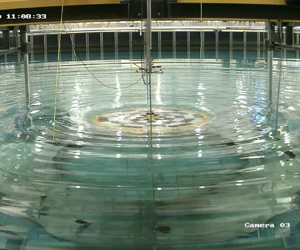
  $b_h$ (predicted by the linear PT flow model). The first heave resonance, which corresponds to a peak in the radiation damping, can be clearly seen. The heave frequencies in the experiments (shown by the crosses) were chosen to span this heave resonance. The vertical lines indicate wave periods (at full scale) of 8 s and 16 s, the expected incident wave period range if the CETO device were to be deployed off the southwest coast of Australia. Figure 6 shows two snapshots of the free surface in experiments for $ka=0.35$, $A/s=0.33$ and $ka=0.60$, $A/s=0.31$, both at $s/a=0.16$. A large water jet at the centre of the cylinder is evident at $ka=0.60$.
Table 1. Experiment parameters.


Figure 5. Frequency-dependent heave radiation damping coefficient  $b_h$ (from linear PT) for the experimental cylindrical geometry at different submergence depths. The experiment test frequencies are shown by the crosses.

Figure 6. Experiment snapshots: (a)  $ka=0.35$, $A/s=0.33$; (b) $ka=0.60$, $A/s=0.31$. Both cases for $s/a=0.16$ and taken just after maximum positive heave displacement. The wave gauge at $r=0$ is fixed to the Qualisys stalk seen in the centre of the cylinder.
5. Comparison with experiments
Force and surface elevation data from experiments are compared to the nonlinear hybrid model, the hybrid model with linearised shallow water equations and a linear PT model for a submerged cylinder as described in Reference McCauley, Wolgamot, Orszaghova and DraperMcCauley et al. (2018) (see § 2 for explanation of each model). The linear potential flow model time-domain results are generated using IRFs for the surface elevation and force given input heave body motion from the experiments.
The heave displacement measured in the experiments by Qualisys is used to force the hybrid model, after a low-pass filter with cut-off at  $6.5\omega$ is used to remove noise from the velocity and acceleration time series (which are calculated from the displacement). The IRFs for the heaving surface-piercing cylinder and the piston are pre-calculated. The surface elevation at the matching boundary due to the heaving surface-piercing cylinder may be calculated for all times as the body velocity is known. However, the convolution integral for the surface elevation at the cylinder edge due to the piston must be evaluated at every time step, as it is dependent on the fluid velocity at the boundary from the shallow water equations solver.
The heave force may be calculated once the piston velocity and surface elevation in the core are known. Impulse response functions for the force on the lower cylinder surface due to motion of the heaving surface-piercing cylinder and the piston are calculated similarly to the surface elevation IRFs shown in § 3.2. The force on the lower cylinder surface also includes a correction for the change in hydrostatic pressure due to the cylinder motion (since the force on the top face is evaluated based on the exact position of the cylinder in time). The force acting on the top cylinder surface is given by integrating the surface elevation from the shallow water solver over the area (i.e. the hydrostatic force).
Figure 7 shows the surface elevation measured above the centre of the cylinder (top row of each panel), cylinder heave displacement measured in the experiments and used to force the hybrid and linear models (middle row of each panel) and the heave hydrodynamic force (bottom row of each panel). Force is defined as positive upwards. Results from three models are shown and the position of the top surface of the cylinder is shown in the top row by the solid black line (except in cases where the free-surface motions are small and the top surface is out of the range plotted). The vertical lines in this figure indicate the predicted arrival time of reflections from the basin sidewalls (calculated using the group velocity of the fundamental frequency); comparison to the left of these lines is therefore most relevant. It can be seen that at high frequency and near the heave resonance (around  $ka=0.6$), the heave motion deviates significantly from the desired sinusoidal signal. As the heave motion was controlled via a taut three-cable arrangement, which could not apply an upward force (the only upward force on the cylinder was from net buoyancy), at high frequencies the required upward velocity was not always reached and the tethers became slack in some cases. Even though the non-harmonic cylinder motion is undesirable, the experimental data nevertheless provide valuable validation since the calculated free-surface and heave force responses are based on the measured motion signals input into the numerical models. We also note that noticeable motion instabilities eventually developed in yaw, pitch and roll at some forcing frequencies (see Reference Orszaghova, Wolgamot, Draper, Taylor and RafieeOrszaghova et al., 2020). However, these built up over longer time scales and therefore did not affect the initial oscillation periods before reflections from the basin walls arrived (maximum rotation in any mode at the time of reflections from the tank walls is 0.64 $^{\circ }$).

Figure 7. Surface elevation at the cylinder centre (top), heave displacement (middle) and heave hydrodynamic force (bottom): (a)  $ka=0.35$, $A/s=0.33$, (b) $ka=0.42$, $A/s=0.34$, (c) $ka=0.60$, $A/s=0.31$, (d) $ka=0.77$, $A/s=0.29$. All plots: $s/a=0.16$, $h/a=2.4$, $T/a=0.4$.
Figure 7 shows larger-amplitude cases ( $A/s = 0.29\unicode{x2013}0.34$) for increasing frequency ( $ka=0.35\unicode{x2013}0.77$) at submergence $s/a=0.16$ (a similar plot for $s/a=0.08$ is given in the supplementary material). The nonlinear hybrid model performs significantly better than the linear PT model in predicting the force in all cases. The linear hybrid model crashes in all cases except at $ka=0.35$, due to the water level (in one or more cells) on the top of the cylinder dropping to zero. This cannot be simulated by the linear shallow water equations model, but can be handled by the wetting and drying scheme implemented in the nonlinear hybrid model. At frequencies above $ka=0.42$ the linear PT model is seen to predict the surface elevation above the cylinder (at $r=0$) to oscillate below the top face of the cylinder, a clear indicator that the model is outside its range of applicability. In all cases the hybrid model provides an improvement over the linear PT model. An estimate of the error in the nonlinear hybrid model and linear PT model total heave force when compared with experimental measurements (for $s/a=0.16$, $50< U<877$) is given in figure 8. The error is calculated as the root-mean-square difference between the experimental force and the linear PT or hybrid model force in the first five oscillations. The value is normalised by the maximum of the experimental force in the same range. It is clear that the nonlinear hybrid model more accurately predicts the heave force for all cases, and that with increasing amplitude the hybrid model performs increasingly better than the linear PT model. Though the nonlinear hybrid model performs significantly better than the linear model, some discrepancy with the experiment remains. Some of this discrepancy may be expected to be associated with viscous losses due to flow around the lower corner of the cylinder and the ‘jet-like’ separation of flow coming off the top of the cylinder. The former problem is common in offshore engineering (e.g. Reference HuseHuse, 1990) while the latter is more unusual. The results indicate that the shallow water flow is indeed the dominant nonlinearity, with acceptable results achieved without attempting to quantify viscous losses. Model–experiment comparisons for the shallower submergence $s/a = 0.08$ are shown in the supplementary material and demonstrate even better performance in this shallower regime.

Figure 8. Root-mean-square (RMS) error in the linear PT and hybrid model force when compared with experiments,  $s/a=0.16$.
It may be seen that the linear hybrid and linear PT models give very similar results in all cases. The deviation between these two models is small compared with the difference between either model and the nonlinear hybrid, and can be attributed to the matching process between the shallow water equations and potential flow components of the hybrid model. Thus, the error introduced by the matching method is not significant compared with the shallow-flow effects in the range tested. The discrepancy between the linear hybrid model and linear PT model is also small compared with the difference between the linear hybrid model and experiments.
Large amplification of the free-surface motion is seen at the centre of the cylinder, observed in experiments as a vertical water ‘jet’ which occurs when a radially converging bore reaches the centre of the core region (see figure 6b). This feature is most pronounced at high frequency (see figure 7c,d), where the wave gauge measurements of the surface elevation are over twice the submergence. The nonlinear hybrid model cannot capture this striking, but very localised, feature of the flow as the shallow water equations do not account for vertical accelerations. However, the hybrid model does capture the arrival of a shock or bore front at a similar time to the jet. There is little evidence from the experiments that the jet significantly affects the total force on the top surface of the cylinder, and at the time at which it occurs the heave force from the hybrid model and the experiments are generally in good agreement.
6. Analysis with harmonic input forcing
Having validated the nonlinear model with experimental data, we now use it (within the range tested) to systematically explore the trends in the heave force for harmonic motion with increasing amplitude. As shown in § 1, calculation of the added mass and damping coefficients has been the focus of much previous work on submerged oscillating structures. It is possible to extract nonlinear heave ‘added mass’ and ‘damping’ coefficients at the fundamental frequency from the hybrid model by isolating the first harmonic of the heave force. In these simulations the cylinder is forced to oscillate harmonically. Once the resulting heave force has reached a steady state, the signal is trimmed (to contain a minimum of eight oscillations) and subsequently band-pass filtered (using  $0.75 \omega$ and $1.25 \omega$ cut-offs) to isolate the first harmonic. The signal is converted back to the time domain and a sine function fitted to determine the linear amplitude and phase of the force. The resulting force coefficients are plotted in figure 9 for submergence $s/a=0.16$ and $0.3< ka<0.8$ against the linear potential flow solution (solid black line). The nonlinear hybrid model results are plotted as solid coloured lines and those of the linear hybrid model as a dashed line, with the colour of the line indicating the amplitude of the heave motion. The linear hybrid model results are independent of amplitude (except at large amplitude where the shallow water equations ‘go dry’ and the model breaks down); thus the result is only plotted for the smallest amplitude.

Figure 9. Nonlinear heave added mass (a) and damping (b) at the fundamental frequency extracted from hybrid and linear PT models. Here  $s/a=0.16$, $h/a=2.4$, $T/a=0.4$.
At low and high frequency both hybrid model solutions tend towards the linear PT solution (but do not reach it due to approximations introduced in the matching; see supplementary material). For small amplitude  $A/s=0.01$ the nonlinear hybrid model agrees well with the linear hybrid model, with small discrepancy in the added mass near the resonance. With increasing amplitude of motion the added mass is reduced for $ka<0.60$ and increased for $ka>0.65$ (though it remains negative in this region). The damping is reduced for $ka>0.55$ and increased for $ka<0.5$, such that we see a shift in the damping peak to lower frequency. The damping peak has shifted from $ka=0.59$ for $A/s=0.01$ to $ka=0.54$ for $A/s=0.4$. For the smaller submergence case where $s/a=0.08$ (not shown for brevity) the effects of increasing amplitude have greater influence on both hydrodynamic coefficients, with a reduction of over 50 % in the damping peak for $A/s=0.2$ as compared with the linear model. Although these plots ignore the higher harmonics in the force, it is clear that the linear model is insufficient for predicting the added mass and damping coefficients where the amplitude of the heave motion is greater than $A/s=0.1$. While obvious, it should be noted that these curves are valuable for illustrating nonlinear changes in behaviour, but cannot be interpreted and used in the way in which linear added mass and damping coefficients are used – the nonlinear time domain model should be used instead.
While examining the nonlinear coefficients at the fundamental frequency helps to relate the hybrid model results to conventional understanding, the full force time histories provide more information; results for four frequencies are plotted in figure 10 for  $A/s=0.01\unicode{x2013}0.5$ and $s/a=0.16$. Changes in the volume of water in the core region (away from the mean) are also plotted for each frequency and amplitude below the corresponding force plot. The coloured vertical lines in each plot correspond to the times of maximum and minimum force for the corresponding amplitude. Free-surface profiles for two frequencies ( $ka=0.35$ and 0.55) and two amplitudes ( $A/s=0.2$ and 0.5) are shown in figure 11. The force on the bottom cylinder surface is generally small relative to the force on the top face, except at low frequency where they are 180 $^\circ$ out of phase, making the second harmonic force component more prominent. Hence, the force on the top face dominates for most frequencies. Three nonlinear effects are particularly noticeable in figure 10:
(i) At each frequency, a delay in the phase of maximum force as the amplitude of oscillation increases, a large effect most important at low frequency.
(ii) At each frequency, a smaller delay in the phase of minimum force as the amplitude of oscillation increases, most apparent around the linear resonance frequency.
(iii) Significant reductions in the amplitude of the maximum and minimum forces as the amplitude of oscillation increases, for frequencies around (linear) resonance.

Figure 10. Total heave force (top row) and change in volume in core region (bottom row): (a)  $ka=0.35$, (b) $ka=0.45$, (c) $ka=0.55$, (d) $ka=0.65$. Heave displacement is plotted on the right-hand axis. The vertical lines indicate the times of maximum and minimum force for each amplitude. All plots: $s/a=0.16$, $h/a=2.4$, $T/a=0.4$.

Figure 11. Free-surface snapshots showing the flow on (top row) and the flow off (bottom row) phases for two amplitudes at (a)  $ka=0.35$ and (b) $ka=0.55$. The arrow represents the direction and amplitude of the velocity at the boundary and the cylinder position for each amplitude is shown by the dashed lines. All plots: $s/a=0.16$, $h/a=2.4$, $T/a=0.4$.
To explain these observations, we divide a cylinder oscillation into two phases: the ‘flow on’ phase (where the fluid velocity at the piston boundary is onto the cylinder) and the ‘flow off’ phase (where the fluid velocity is off the cylinder). The flow on phase starts with a shallow flow propagating onto the cylinder and ends when the reflection from the cylinder centre propagates off the edge, at the same time as (or just after) the minimum in force occurs (corresponding to maximum fluid on the cylinder). For large-amplitude oscillations, the shallow flows on the cylinder dominate during the flow off phase. The strong flow off acts to delay the reversal of flow at the boundary and results in a phase delay in the maximum force with increasing amplitude. This partly explains observation (i), which is also influenced by the second harmonic at low frequency. Observation (ii) suggests that despite starting later, during the flow on, the bores at larger amplitude reflect from the centre and back to the edge more quickly, a nonlinear effect. At higher frequencies ( $ka>0.35$) the cylinder is already moving upwards when flow off starts. The surface elevation on the cylinder near the centre drops to zero (or close to) as it starts to move downwards (see figure 11b), resulting in a minimum in the fluid volume on top of the cylinder and a maximum in the force. For larger amplitudes and at higher frequency the cylinder is almost completely dry on top, such that the non-dimensional peak in force must be reduced with amplitude, as the volume of fluid on the cylinder does not scale. Similarly, at higher frequency the cylinder is closer to the mean free surface (relative to the amplitude) when the maximum volume occurs, resulting in a reduction in the volume of fluid on top of the cylinder (see figure 11b). Hence the force on the top cylinder surface cannot scale linearly with amplitude. Thus the maximum and minimum force reductions in observation (iii) are explained.
The phase shift in the peak force at low frequency results in the increase in nonlinear damping with amplitude observed earlier, since the force is closer to the phase of the velocity. However, at higher frequencies ( $ka>0.45$) the decrease in relative magnitude of the force with increasing amplitude overcomes the phase shift and the damping decreases with increasing amplitude.
7. Discussion and conclusions
The nonlinear hybrid model developed in this work compares well with experiments for the Ursell number range  $2.5< U<1061$ and provides significant improvement over linear potential flow theory for predicting the heave force for large-amplitude forced heave motion. The improvement is even more apparent for the shallower of the two submergence cases tested, for which the model is particularly well suited. The hybrid model cannot model the vertical water jet at the centre of the core region, but does capture the arrival of a steep-fronted wave at the centre of the cylinder at a similar time to the jet. Thus it appears that the bulk flow in the shallow water region is captured correctly by the model, and that the jet has a minor effect on the heave force. Comparisons of nonlinear added mass and damping coefficients at the fundamental frequency from the hybrid model to the full linear potential flow model indicate that the heave motion amplitude has significant impact on the force coefficients. For heave amplitude of half the submergence depth (i.e. $A/s=0.5$) the damping may be reduced by a factor of 2 and the peak shifted to lower frequency. This, of course, does not take into account the higher frequency components of the force, but is a clear indication that the linear model is inaccurate where the cylinder heave motions are larger than $A/s=0.1$. A similar trend in the added mass and damping was identified in the CFD simulations of a heaving cylinder by Reference Rafiee and ValizadehRafiee and Valizadeh (2018) and in the experiments of Reference Molin, Remy and RippolMolin, Remy, and Rippol (2007), who tested submerged disks oscillating in heave ( $0.12< U<463$). This has significant implications for development of shallowly submerged wave energy devices, and indicates that power predictions or design decisions based on linear hydrodynamic models will be inaccurate, and that a nonlinear model is required. Given that the present model can predict heave force with reasonable accuracy and with greatly reduced computation time compared with CFD (a 100 s simulation takes 495 s on a four-core CPU), the hybrid model shows promise for application to the full problem, i.e. where other modes of motion are included and the model is forced by incident waves. Recent work on submerged wave energy convertors (Reference Tran, Sergiienko, Cazzolato, Ding, Wuillaume, Ghayesh and ArjomandiTran et al., 2021; Reference Tran, Sergiienko, Cazzolato, Ghayesh and ArjomandiTran, Sergiienko, Cazzolato, Ghayesh, & Arjomandi, 2022) suggests that mode coupling is of high importance in power absorption – there would be great value in extending the weakly nonlinear model used in these works to a hybrid model taking better account of shallow water effects. However, this requires further model development and validation experiments.
Supplementary material
Supplementary material is available at https://doi.org/10.1017/flo.2023.32. The experimental data are commercially confidential and not available to the public.
Acknowledgements
The authors would like to acknowledge Professor R. Eatock Taylor for his many helpful suggestions concerning this work.
Funding statement
G.M. would like to acknowledge funding from the Robert and Maude Gledden Scholarship. G.M., H.W. and S.D. acknowledge the kind support of the Lloyds Register Foundation. The Lloyds Register Foundation supports the advancement of engineering related education, and funds research and development that enhances safety of life at sea, on land and in the air. H.W. is supported by an Australian Research Council (ARC) Early Career Fellowship (DE200101478). This work forms part of the activities conducted within the ARC Linkage Project 150100598. The laboratory tests were undertaken by the University of Western Australia in collaboration with Carnegie Clean Energy at the COAST laboratory at the University of Plymouth, UK, and were supported by MaRINET2 funding.
Declaration of interests
The authors declare no conflict of interest.
Author contributions
The Plymouth experiments were conducted by J.O., H.W. and G.M. (with the help of others). G.M. developed the hybrid models, conducted the analysis and wrote the manuscript. H.W., S.D. and J.O. assisted with the analysis, model development and reviewed the manuscript.


 Open access