


Impact Statement
Ongoing development of experimental turbulence facilities enables the study of fascinating fluid dynamics phenomena and aids in the understanding of fundamental transport mechanisms. Generating zero-mean-flow homogeneous isotropic turbulence (HIT) in the laboratory is challenging and requires careful tuning of the experimental set-up. Each facility designed to produce HIT incorporates distinct features. This review summarizes the design and operation of several types of laboratory facilities that generate incompressible zero-mean-flow HIT, and provides a new meta-analysis relating facility size and energy injection methods to resulting turbulence properties across facility types. Understanding the capabilities and limitations of such facilities is also useful for those who use numerical simulations to understand complex fluid phenomena – both for validation of numerics and for planning and executing collaborations with experimentalists. With this compiled information as a resource, researchers can design well-tuned turbulence facilities that enable new advances in experimental fluid dynamics.
1. Introduction
Turbulence is important in environmental and industrial flows due to its impact on processes such as mixing, sediment transport and air–water interaction. Turbulence influences circulation in the ocean and the atmosphere, enhances the effective diffusivity of substances in the environment, drives sediment morphology and affects the health and survival of many living creatures. Numerical, laboratory and field studies have contributed to our understanding of turbulent flow. However, the stochastic nature of turbulence presents a unique challenge to repeatability and cross-comparison between flows (Reference PopePope 2000).
Laboratory studies provide a systematic way to isolate particular phenomena that may be more challenging to pursue via field studies or numerical simulations. Field conditions are difficult to control, due to the complexity of interactions between various drivers of flow. This can impede parametric exploration of desired variables. Numerical simulations, while rapidly increasing in capability, are still constrained by computational cost and challenges regarding imposing appropriate boundary conditions. Even laboratory-generated turbulence can be challenging to compare from one facility to another. It is therefore of interest to experimentally generate turbulence that is as free as possible from the signature of boundaries and forcing mechanisms, so that fundamental processes can be investigated across different facilities.
In most environmentally or industrially relevant flows, turbulence is neither homogeneous (statistically independent of spatial position) nor isotropic (statistically independent of orientation). Differences in boundary conditions or driving forces can dramatically change the characteristics of the resulting flow. However, the study of homogeneous and isotropic turbulence (HIT) can serve as a crucial starting point for improving our understanding of the energetics and transport potential of such flows, allowing us to simplify and generalize conclusions to yield more fundamental insight, and assess long-standing fundamental hypotheses in turbulence, such as Kolmogorov's hypothesis (Reference BatchelorBatchelor 1953; Reference Lawson, Bodenschatz, Knutsen, Dawson and WorthLawson et al. 2019; Reference Marston and TobiasMarston & Tobias 2022). Many specialized laboratory facilities have been developed to accomplish this. In this review, we discuss the history of HIT generation, presently existing facilities and their operation, challenges and opportunities presented by various approaches and overall best practices for generating HIT in the laboratory.
1.1 History of laboratory-generated HIT
1.1.1 Wind and water tunnels
The first purpose-designed HIT-generating facilities were wind (Reference Simmons and SalterSimmons & Salter 1934; Reference Comte-Bellot and CorrsinComte-Bellot & Corrsin 1966) and water (Reference Gibson and SchwarzGibson & Schwarz 1963) tunnels. These facilities used a static, passive grid located upstream of the test section, causing HIT to develop downstream due to the interaction of wakes behind the grid. Reference MakitaMakita (1991) introduced the ‘active grid’, in which protruding wings rotate at intervals to randomly block portions of the grid. This approach generated turbulence at a higher Reynolds number as compared with a passive grid. A review of active grids was recently published by Reference MydlarskiMydlarski (2017); both passive and active grids are used in modern facilities.
Reference Uzkan and ReynoldsUzkan & Reynolds (1967) modified passive-grid water tunnels to study mean-shear-free turbulence. They used a mobile bed, moving at the same speed as the streamwise velocity, to eliminate the mean velocity gradient (i.e. mean shear) at the bed. Similar experiments by Reference Thomas and HancockThomas & Hancock (1977) and Reference Aronson, Johansson and LöfdahlAronson, Johansson & Löfdahl (1997) generated high-Reynolds-number mean-shear-free turbulence via a passive grid in a wind tunnel, eliminating the mean boundary-layer-generated velocity gradient by moving the bed at the mean velocity of the flow. These mean-shear-free tunnel studies highlighted the underlying effects of boundaries in isolation of any mean velocity gradient; they were later used for validation and development of theories regarding the fundamental role of turbulence near boundaries (Reference Hunt and GrahamHunt & Graham 1978; Reference Biringen and ReynoldsBiringen & Reynolds 1981; Reference HuntHunt 1984; Reference Perot and MoinPerot & Moin 1995; Reference Walker, Leighton and Garza-RiosWalker, Leighton & Garza-Rios 1996).
While eliminating mean shear gives insight into fundamental processes of turbulence, there is also value in removing mean flow. By removing mean flow, the complexities and uncertainties that arise in both natural and industrial environments are significantly reduced, offering a unique opportunity to isolate and investigate the physical driving mechanisms related to turbulent flow. For the study of multiphase flows, for example, zero-mean-flow turbulence can increase the feasible observation time of suspended bubbles, drops and particles, enabling Lagrangian analysis (Reference Toschi and BodenschatzToschi & Bodenschatz 2009). In recent years, several turbulence facilities have been developed to generate HIT while minimizing the mean (background) flow or presence of recirculating currents. These facilities typically apply forcing via grids, fans, jets, loudspeakers or other point-source agitators.
1.1.2 Grid-stirred tanks
Reference Rouse and DoduRouse & Dodu (1955) developed the grid-stirred tank (GST), intended to generate HIT with neither recirculation nor mean shear via a planar grid oscillating along an axis normal to the grid plane. As the grid reciprocates linearly, its successive wakes interact to create HIT. Because of their simple design, low cost and relative ease of use, GSTs have remained popular for generating HIT in laboratories and are still in use today (e.g. Reference Thompson and TurnerThompson & Turner 1975; Reference Brumley and JirkaBrumley & Jirka 1987; Reference McCorquodale and MunroMcCorquodale & Munro 2018). Properties of GST-generated turbulence depend strongly on grid characteristics, such as solidity (percent open area), rod/bar diameter and oscillation frequency (e.g. Reference Thompson and TurnerThompson & Turner 1975; Reference Hopfinger and TolyHopfinger & Toly 1976; Reference McDougallMcDougall 1979; Reference NokesNokes 1988). The distance from the grid to the homogeneous and isotropic region is also a function of the grid geometry; Reference Hopfinger and TolyHopfinger & Toly (1976) and Reference Thompson and TurnerThompson & Turner (1975) determined that the developed isotropic region starts at a distance twice the mesh size (rod-to-rod spacing) away from the grid. This distance allows the wakes generated by the oscillating grids to decay and expand, ultimately interacting to generate HIT (Reference Dohan and SutherlandDohan & Sutherland 2002).
Grid-stirred tanks have frequently been used to investigate the effects of turbulence on environmental phenomena, including heat and mass flux across density interfaces (Reference Thompson and TurnerThompson & Turner 1975; Reference Hopfinger and TolyHopfinger & Toly 1976; Reference Xuequan and HopfingerXuequan & Hopfinger 1986; Reference NokesNokes 1988; Reference Kit, Strang and FernandoKit, Strang & Fernando 1997; Reference Holzner, Liberzon, Guala, Tsinober and KinzelbachHolzner et al. 2006), gas transfer across a free surface (Reference JirkaJirka 2008), sediment transport and resuspension (Reference Tsai and LickTsai & Lick 1986; Reference Medina, Sánchez and RedondoMedina, Sánchez & Redondo 2001; Reference Orlins and GulliverOrlins & Gulliver 2003), flocculation (Reference Casson and LawlerCasson & Lawler 1990; Reference Cuthbertson, Dong and DaviesCuthbertson, Dong & Davies 2010), flow through vegetation (Reference Pujol, Colomer, Serra and CasamitjanaPujol et al. 2010), particle-laden flow (Reference Ni, Kramel, Ouellette and VothNi et al. 2015) and many more. However, these facilities have some limitations. While intended to eliminate mean flow, GSTs have consistently been shown to exhibit overturning mean circulations and secondary flows at or above the scale of the turbulent fluctuations, a result of mass conservation (Reference CromwellCromwell 1960; Reference Srdic, Fernando and MontenegroSrdic, Fernando & Montenegro 1996; Reference Mann, Ott and AndersenMann, Ott & Andersen 1999; Reference Dohan and SutherlandDohan & Sutherland 2002; Reference McKenna and McGillisMcKenna & McGillis 2004). In other words, secondary flows are inherent to GSTs due to the uniform planar forcing combined with the presence of relatively nearby boundaries. Reproducing a specific flow in these facilities is also challenging, since the generated flow is highly dependent on the initial condition and location of the grid (Reference Xuequan and HopfingerXuequan & Hopfinger 1986; Reference McKenna and McGillisMcKenna & McGillis 2004).
Several modifications have improved the performance of GSTs. Placing two parallel grids at opposite ends of the tank instead of using only one oscillating grid was found to improve isotropy and reduce the rate of decay (Reference Villermaux, Sixou and GagneVillermaux, Sixou & Gagne 1995; Reference Shy, Jang and TangShy, Jang & Tang 1996; Reference Srdic, Fernando and MontenegroSrdic et al. 1996; Reference Shy, Tang and FannShy, Tang & Fann 1997; Reference Yang and ShyYang & Shy 2003; Reference Zellouf, Dupont and PeerhossainiZellouf, Dupont & Peerhossaini 2005). Near the grids, the wakes generated are similar to those observed in single-grid facilities (Reference Shy, Jang and TangShy et al. 1996); however, the symmetric forcing generates HIT in the central region with a smaller decay rate compared with single-grid facilities (Reference Zellouf, Dupont and PeerhossainiZellouf et al. 2005). The use of two grids also provides the opportunity to agitate both layers in a two-layer fluid system (Reference Mcgrath, Fernando and HuntMcgrath, Fernando & Hunt 1997). Reference Li, Zhang, Yang, Fu and XiaoLi et al. (2020) used two pairs of parallel grids (i.e. four grids in total oscillating along a common axis) to enhance the fluctuating velocity in the direction of oscillation and reduce flow inertia normal to the oscillation axis, therefore mimicking a turbulent channel flow while maintaining minimal background flow. Some experiments used five or six oscillating grids in a single tank (Reference Casson and LawlerCasson & Lawler 1990; Reference BrunkBrunk 1996); Reference Dickinson and LongDickinson & Long (1983) placed a small tank inside of a larger tank with one oscillating grid located in the larger tank to reduce recirculations. Even though the use of multiple grids has decreased these recirculations, the dependence of turbulence characteristics on large-scale motions in GSTs (Reference Blum, Kunwar, Johnson and VothBlum et al. 2010) led to a need to further decrease mean flow.
1.1.3 Synthetic jets and pointwise energy injection
While GSTs have achieved acceptable levels of homogeneity and isotropy for some applications, each grid still imparts momentum primarily in the grid-normal direction. This can lead to unavoidable anisotropy and to large-scale secondary (background) flows. As an alternative, pointwise energy injection, for example via synthetic jets, can reduce mean background flow and subsequent mean shear. Synthetic jets introduce momentum without a concomitant mass flux (Reference Smith and GlezerSmith & Glezer 1998; Reference Glezer and AmitayGlezer & Amitay 2002), and can include fans, loudspeakers, propellers and bilge pumps. These actuators can be placed at the corners and/or along the walls of experimental facilities. The induced flows subsequently interact to form a central HIT region with small mean flow. Recent innovative techniques have also been developed to generate turbulence in laboratories via injection of vortex rings and magnetic particles (Reference Gorce and FalconGorce & Falcon 2022; Reference Matsuzawa, Mitchell, Perrard and IrvineMatsuzawa et al. 2023). We note that some facilities use rotating elements (e.g. counter- or co-rotating disks) to generate a swirling flow in the tank with a relatively small region of negligible mean flow (e.g. Reference Douady, Couder and BrachetDouady, Couder & Brachet 1991; Reference Fauve, Laroche and CastaingFauve, Laroche & Castaing 1993; Reference Voth, Porta, Crawford, Alexander and BodenschatzVoth et al. 2002; Reference Ouellette, Xu, Bourgoin and BodenschatzOuellette et al. 2006; Reference Klein, Gibert, Bérut and BodenschatzKlein et al. 2012; Reference Webster and YoungWebster & Young 2015; Reference Ye, Manning and HsuYe, Manning & Hsu 2020). These facilities, sometimes called ‘French washing machines’, or ‘von Kármán swirling tanks’, reproduce important elements of turbulence but typically have strong mean flow outside of this small central region; therefore, they are not the focus of the present discussion. Other studies have used rotating elements such as grids and disks (with and without random forcing) to generate non-swirling, zero-mean-flow HIT (Reference Liu, Katz and MeneveauLiu, Katz & Meneveau 1999; Reference Bordoloi, Verhille and VarianoBordoloi, Verhille & Variano 2019; Reference Pujara, Clos, Ayres, Variano and Karp-BossPujara et al. 2021). Random forcing, coupled with the use of many rotating objects, reduces the strongly persistent vorticity that is otherwise characteristic of rotating-element-driven flow.
Synthetic jets are often used in planar arrays, which are more compatible with standard rectangular tanks than corner-mounted approaches (which typically require highly customized tank geometry). This creates momentum flux normal to the plane, as oscillating grids do; however, the jets are typically driven in a spatiotemporally varying pattern, unlike an oscillating grid. Random jet arrays (RJAs), introduced by Reference Variano, Bodenschatz and CowenVariano, Bodenschatz & Cowen (2004), are capable of generating HIT with high Reynolds number and negligible mean flow or boundary shear. Mean flows in facilities using RJAs (e.g. Reference Variano and CowenVariano & Cowen 2008; Reference Pérez-Alvarado, Mydlarski and GaskinPérez-Alvarado, Mydlarski & Gaskin 2016; Reference Johnson and CowenJohnson & Cowen 2018) are among the lowest reported relative to alternative turbulence-generation mechanisms. In a RJA, synthetic jets are organized within a Cartesian-grid array, and they are randomly turned on and off according to specified forcing parameters. This stochasticity prevents the formation of persistent mean recirculation. The choice of a single or multiple array implementation, along with opportunities to tune the algorithm parameters, gives ample flexibility to optimize turbulence generation for a given application.
Here we have provided a brief overview of the historical development of incompressible zero-mean-flow HIT facilities. In the following sections, we explore these facilities in detail, focusing on the dynamic forcing mechanisms that came into use after the development of GSTs. In § 1.2, we provide a brief primer on the turbulent flow characteristics considered throughout the referenced studies to ensure consistent definitions and notation. In § 2, we explore the various flow-producing devices (i.e. fans, loudspeakers, jets and rotating elements) used in existing HIT facilities. Section 3 is devoted to synthesis and commentary on the characteristics of turbulent flow generation across different types of facilities. Finally, § 4 provides an overall summary of the present state of laboratory-generated zero-mean-flow HIT, as well as some guidelines for those seeking to construct new facilities.
1.2 Turbulence characteristics
To compare the performance of turbulence-generating facilities, we first define the parameters typically used to quantify turbulent flow. To establish notational consistency, here we present definitions for the most common parameters used across the included studies (and further note that this list is non-exhaustive). In table 1, bold text represents vector quantities. The subscripts  $i$,
$i$,  $j$ and $k$ can take on values corresponding to any of the three Cartesian coordinate directions.
Table 1. Common turbulent flow parameters used throughout the review. All definitions are taken from Reference PopePope (2000) and Reference Tennekes and LumleyTennekes & Lumley (1972).

In many of the facilities discussed below, symmetry is used to justify calculating parameters with two-dimensional flow data (e.g.  $u$ and $w$ instead of $u$,
$u$,  $v$ and $w$). For instance, in cases of planar forcing via a single jet array in the $x$–
$x$– $y$ plane, radial symmetry applies and $k$ can be calculated as $k = \frac {1}{2} (2u'^2 + w'^2)$. Similarly, the direct calculation of $\epsilon$ can be simplified from nine velocity gradients to four given assumptions of continuity, symmetry and isotropy (Reference Doron, Bertuccioli, Katz and OsbornDoron et al. 2001; Reference Johnson and CowenJohnson & Cowen 2018). While we present isotropy as the ratio of RMS velocities (as in table 1), we note that isotropy can also be quantified via the ratio of integral length scales, where ${\mathcal {L}_L}/{\mathcal {L}_T}=2$ indicates isotropy. These two ratios have sometimes indicated different degrees of isotropy (e.g. Reference Carter and ColettiCarter & Coletti 2017; Reference Johnson and CowenJohnson & Cowen 2018). Here we use $\varOmega _{ij}$ because it is most commonly reported among the reviewed literature. We further emphasize that there are multiple methods for measuring the degree of isotropy of a given flow, but there is no standard test or threshold for declaring a particular flow to be isotropic or anisotropic. Parameters such as $\varOmega _{ij}$ are helpful in that they assist in comparing facilities.
2. Actuator-based turbulence-generation mechanisms
In this section, we consider four types of forcing mechanisms (actuators) in order to explore their influence on flow generation and turbulence characteristics: fans, loudspeakers, jets and other rotating elements. Forcing may be steady, in which the actuators are active continuously, or unsteady, in which the actuators follow stochastic or deterministic time-varying patterns. Some actuators are better suited for only one working fluid (typically air and water), while others can be used in either gases or liquids. We compare how modifications to the operation and configuration of these actuators alter the resulting flow, and discuss practical drawbacks and advantages of each type of actuator. Most of the facilities discussed in this section, along with their turbulence characteristics, are presented in the Appendix (table 6).
2.1 Fan-driven turbulence generation
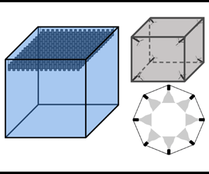
Homogeneous isotropic turbulence can be generated by placing several fans symmetrically about a central region, typically at the vertices of the facility, so that their momentum combines to generate HIT. The number of fans can vary, with a minimum number of four among the surveyed facilities. The rotational speed of the fans is typically kept constant during a single experiment (steady forcing). However, stochastic forcing can also be incorporated to modify the flow statistics and dependence on the forcing mechanism, as was recently done in a planar impeller array (Reference Lawson and GanapathisubramaniLawson & Ganapathisubramani 2022). Fan-driven facilities have been used to investigate the effects of turbulence on combustion (Reference SemenovSemenov 1965; Reference Andrews, Bradley and LwakabambaAndrews, Bradley & Lwakabamba 1975; Reference Fansler and GroffFansler & Groff 1990; Reference Xu, Huang, Huang, Wei, Cheng, Ma and ZhangXu et al. 2017), preferential particle concentration in microgravity (Reference Fallon and RogersFallon & Rogers 2002), particle clustering (Reference Salazar, Jong, Cao, Woodward, Meng and CollinsSalazar et al. 2008; Reference Fiabane, Zimmermann, Volk, Pinton and BourgoinFiabane et al. 2012, Reference Fiabane, Volk, Pinton, Monchaux, Cartellier and Bourgoin2013) and vaporization of chemicals and water droplets (Reference Birouk, Chauveau, Sarh, Quilgars and GökalpBirouk et al. 1996; Reference Birouk and GökalpBirouk & Gökalp 2002; Reference Li, Lohse and HuismanLi, Lohse & Huisman 2023). Table 2 summarizes some properties of fan-driven facilities that generate HIT with a negligible mean flow. Such facilities are usually small ( ${<}1$ m) in size, with a symmetric forcing geometry. An example of fan-driven facility with a possible fan structure is shown in figure 1.
Table 2. Characteristics and flow statistics of fan-driven turbulence facilities, where  $f$ is rotational fan speed and other variables are defined in § 1.2. Parameter $D_{fan}$ is the diameter of the fan. Note that throughout the following sections, $\mathcal {L}$ is shown with $^{{*}}$ and $\mathcal {L}_L$ is shown with $^{{+}}$. The superscript $^{{\times }}$ indicates values estimated by the authors from provided data. Note that in the study of Reference Ravi, Peltier and PetersenRavi, Peltier & Petersen (2013) multiple fan configurations were used; the result shown is for the baseline fan prototype.


Figure 1. (a) Schematic of a cuboidal fan facility with height  $H$, width $W$ and length $L$. (b) Schematic of a fan with three blades.
2.1.1 Fan configurations
Fan structural properties (e.g. number of blades, blade pitch angle ( $\theta$), fan diameter) and rotational speed can have strong effects on the generated turbulent flow (e.g. Reference Kwon, Wu, Driscoll and FaethKwon et al. 1992; Reference Gillespie, Lawes, Sheppard and WoolleyGillespie et al. 2000; Reference Kumaresan and JoshiKumaresan & Joshi 2006; Reference Ravi, Peltier and PetersenRavi et al. 2013). According to Reference Ravi, Peltier and PetersenRavi et al. (2013), increasing the blade pitch angle and number of blades decreases turbulent Reynolds number, integral length scale, isotropy and homogeneity, but increases overall turbulent kinetic energy in the HIT region. The dissipation rate was unaffected by the number of blades, but it increased substantially when the pitch angle increased. This may be due to stronger axial momentum input at higher pitch angles, which leads to a decrease in both isotropy and homogeneity in the central volume. Their results show that changing the rotational frequency in fan-driven facilities does not affect the value of $\mathcal {L}_L$.
In fan-generated HIT, the magnitudes of the fluctuating velocities can be increased by increasing the rotational frequency ( $f$) of the fans. Reference Dou, Pecenak, Cao, Woodward, Liang and MengDou et al. (2016) proposed that turbulence strength (similar to $u_T$; see table 1) is linearly correlated with $f$, and $Re_{\lambda }$ is proportional to the square root of fan speed. Similarly, Reference Birouk, Sarh and GökalpBirouk et al. (2003), Reference Zimmermann, Xu, Gasteuil, Bourgoin, Volk, Pinton, Bodenschatz and ResearchZimmermann et al. (2010) and Reference Bradley, Lawes and MorsyBradley et al. (2019) detected a linear relationship between the turbulent fluctuating velocities and $f$ (figure 2), albeit with slightly different slopes. This linear relationship between $u'$ and $f$ implies that the fluctuating velocities scale with the tip speed of the fan, although the precise scaling likely depends on the facility and fan geometry. However, changing $f$ did not modify the integral length scales (Reference Gillespie, Lawes, Sheppard and WoolleyGillespie et al. 2000; Reference Bradley, Lawes and MorsyBradley et al. 2019). The overall geometry of fan-driven facilities is more influential on $\mathcal {L}_L$ than either the fan structure or rotational speed, as we discuss in § 3.3. Reference Leisenheimer and LeuckelLeisenheimer & Leuckel (1996) explored the effects of vessel size, number of fans and fan diameter on the generated HIT. They concluded that the vessel size was the main contributor to the value of the integral length scale, and proposed a linear relationship between $\mathcal {L}_L$ and the radius of the facility.

Figure 2. (a) Changes to  $u'$ with respect to the fan speed, using data from Reference Birouk, Sarh and GökalpBirouk et al. (2003) ( $\bullet$) and Reference Bradley, Lawes and MorsyBradley et al. (2019) ( $+$). (b) Values of skewness ( $\small {\bullet }$) and kurtosis ( $+$) of $u'$ with a Gaussian-fitted distribution when changing fan speed, using data from Reference Bradley, Lawes and MorsyBradley et al. (2019).
Reference Bradley, Lawes and MorsyBradley et al. (2019) found that while  $\mathcal {L}_L$ remains constant with increasing fan speed, integral time scale, $\tau$, a characteristic eddy turnover time scale, decreases while RMS velocity increases. This can be understood via a dimensional argument: at large length scales, viscosity is not important, so the forcing frequency provides the only inherent time scale of $1/f$. Thus, for a given fan structure, $\tau$ decreases as $f$ increases while $\mathcal {L}_L$ remains constant (since the inherent length scales of fan diameter, facility size and fan spacing do not change with $f$). Increasing $f$ produced a smaller region of HIT, and altered the normality of the distribution of the fluctuating velocities (Reference Ravi, Peltier and PetersenRavi et al. 2013; Reference Bradley, Lawes and MorsyBradley et al. 2019) (figure 2). Reference Bradley, Lawes and MorsyBradley et al. (2019) observed that the largest, most homogeneous and most isotropic region of HIT in their studies occurred when $f$ was set to a value between 2000 and 4000 r.p.m. (similar to Reference Birouk, Sarh and GökalpBirouk et al. (2003)).
2.1.2 Advantages and drawbacks
Since the HIT region is generated as a result of the interactions between local vortical flows induced by each fan, its characteristics and RMS velocities vary with respect to these local motions and fan structures. One advantage of these facilities is that an increase in the magnitude of the fluctuating velocities does not necessarily correspond to an increase in the background mean flow. The mean flow is negligible in most studies presented in this section, and the volume of the HIT region is fairly small (less than approximately 10 % of the facility size, as determined from measurements such as planar particle image velocimetry). In fan-driven facilities, an increase in the magnitude of the RMS velocities does not necessarily correspond to an increase in the mean velocity. Therefore, although the HIT region is small, the mean flow within that region remains negligible. Another advantage of this type of facility is that the time required for the flow to reach steady state from initiation of fan motion is small (e.g. 10 s for Reference Dou, Pecenak, Cao, Woodward, Liang and MengDou et al. (2016)), because the values of  $\tau$ in these facilities are relatively small (e.g. <20 ms for Reference Bradley, Lawes and MorsyBradley et al. (2019)). In general, the turbulent flow characteristics are relatively consistent across all of the fan facilities presented here. Flows generated via fans are highly reproducible and do not depend significantly on initial conditions.
2.2 Loudspeaker-forced turbulence
Acoustic actuators, such as loudspeakers, have been used as synthetic jets to generate HIT. As with fan-driven facilities, the actuators are mounted symmetrically around a central region in which HIT is created. In each loudspeaker a diaphragm of diameter  $d_L$ placed in a cavity vibrates sinusoidally with frequency $F$ and a specific phase, which can be deterministic (constant frequency and phase) or stochastic (variable frequency within an experiment). In front of the cavity, various orifices (usually circular with a specific diameter $d_J< d_L$) are placed to produce jet-like motion via mass conservation within the cavity. The frequency and phase of the inputs are tuned to diminish the generation of secondary flows or standing waves in the tank, as well as to reduce return flows that form due to mass conservation within the larger chamber when the apparatus is closed (Reference Lu, Fugal, Nordsiek, Saw, Shaw and YangLu et al. 2008; Reference Sabban and van HoutSabban & van Hout 2011; Reference Hoffman and EatonHoffman & Eaton 2021). As introduced in § 1.1.3, stochastic forcing diminishes mean flow by disrupting large-scale recirculation. In unbounded, open-air facilities (e.g. that of Reference Goepfert, Marié, Chareyron and LanceGoepfert et al. 2010), stochastic forcing is not needed to avoid mean flow (see § 3.2 and figure 3). Loudspeaker-driven HIT with zero mean flow has been used to study phenomena including pollen dispersal in turbulent air (Reference Sabban and van HoutSabban & van Hout 2011), particle movements and trajectories (Reference Sabban, Cohen and van HoutSabban, Cohen & van Hout 2017), ice melting in turbulence (Reference Stapountzis, Dimitriadis, Giourgas and KotsanidisStapountzis et al. 2015) and zooplankton in oceanic turbulence (Reference Webster, Brathwaite and YenWebster, Brathwaite & Yen 2004; Reference DiBenedetto, Helfrich, Pires, Anderson and MullineauxDiBenedetto et al. 2022). Table 3 summarizes some properties of loudspeaker-driven facilities that generate zero-mean-flow HIT.

Figure 3. Loudspeaker facility. Reproduced from Reference Goepfert, Marié, Chareyron and LanceGoepfert et al. (2010).
Table 3. Geometry and turbulence characteristics of loudspeaker-driven facilities. Parameter  $L_S$ indicates distance between the speakers for the unbounded facility of Reference Goepfert, Marié, Chareyron and LanceGoepfert et al. (2010). Note that in the study of Reference Chang, Bewley and BodenschatzChang, Bewley & Bodenschatz (2012), multiple $\varOmega$ with the same $Re_{\lambda }$ were studied; here we only include results for the value of $\varOmega \approx 1$. The remaining superscripts are explained in table 2.

2.2.1 Loudspeaker characteristics
As with fan-driven facilities, loudspeaker-driven facilities can generate HIT with low mean flow; for example, Reference Hwang and EatonHwang & Eaton (2004) measured an HIT area of  $4\,{\rm cm}\times 4\,{\rm cm}$ via planar particle image velocimetry in their facility. To improve turbulence characteristics, various barriers may be placed in front of the loudspeakers. For example, Reference Hwang and EatonHwang & Eaton (2004) placed a mesh along the speaker faces to break down the large-scale fluid structures generated by the loudspeaker, thereby introducing intermediate length scales. Reference Goepfert, Marié, Chareyron and LanceGoepfert et al. (2010) and Reference Webster, Brathwaite and YenWebster et al. (2004) used plates with a lattice of smaller holes, which forced flow into higher-velocity jets. This structure provided a high outlet velocity and a uniform momentum flux without a significant pressure change.
Increasing the amplitude of the speakers directly affects the fluctuating velocity, dissipation rate and turbulent kinetic energy (Reference Webster, Brathwaite and YenWebster et al. 2004; Reference Sabban and van HoutSabban & van Hout 2011; Reference Hoffman and EatonHoffman & Eaton 2021). Reference Webster, Brathwaite and YenWebster et al. (2004) showed that increasing the amplitude of the input signal of the loudspeakers improved  $\varOmega$ and increased $Re_{\lambda }$. Reference Sabban and van HoutSabban & van Hout (2011) observed the same behaviour, along with increased $k$ and slightly decreased mean flow. Increasing speaker amplitude (and therefore $Re_\lambda$) leads the probability density function of the fluctuating velocities to fall closer to a Gaussian distribution. However, at a somewhat higher Reynolds number ( $Re_{\lambda }>165$), Reference Hoffman and EatonHoffman & Eaton (2021) did not observe any significant changes in $\varOmega$ or mean flow strength with increasing loudspeaker input power.
2.2.2 Advantages and drawbacks
As in fan-driven facilities, loudspeakers may be actuated individually to tune the generated flow and create intentional anisotropy. Some configurations allow for modification of the fluctuating velocities without changing the Reynolds number or the mean flow generated in the facility (e.g. Reference Bewley, Chang and BodenschatzBewley, Chang & Bodenschatz 2012; Reference Chang, Bewley and BodenschatzChang et al. 2012; Reference Bewley, Saw and BodenschatzBewley, Saw & Bodenschatz 2013). Using a scaling argument, Reference Hoffman and EatonHoffman & Eaton (2021) proposed that loudspeaker-driven facilities can be designed based on the desired Reynolds number and dissipation rate, providing a flexible platform to generate HIT. Similar to fan-driven facilities, the time to reach an equilibrium turbulent state in loudspeaker-driven turbulence is short (e.g. 60 s for Reference Lu, Fugal, Nordsiek, Saw, Shaw and YangLu et al. (2008)).
On the downside, Reference Hoffman and EatonHoffman & Eaton (2021) found it challenging to generate HIT with negligible mean flow. This is an indication of the importance of the physical characteristics of the chamber with respect to the generated turbulence (see § 3.3). Additionally, the homogeneous isotropic region is small, even when the facility is large; for example, the apparatus used by Reference Bewley, Chang and BodenschatzBewley et al. (2012) exhibited a region of HIT of only 50 mm in diameter despite a facility inner diameter of 1 m.
2.3 Turbulence generation via jet arrays
Another mechanism for generating HIT with negligible mean flow, introduced by Reference Variano, Bodenschatz and CowenVariano et al. (2004), is the RJA. Jets, organized in a planar array at a distance  $S$ from one another, are stochastically turned on and off to generate HIT at some distance from the jet plane. Often, such arrays use submersible pumps that accelerate fluid effectively from a point (injecting only momentum, not mass, in keeping with the definition of a synthetic jet). In other instances, pressure opening valves are used to produce the momentum needed for HIT generation (Reference Variano, Bodenschatz and CowenVariano et al. 2004; Reference Carter, Petersen, Amili and ColettiCarter et al. 2016; Reference Esteban, Shrimpton and GanapathisubramaniEsteban, Shrimpton & Ganapathisubramani 2019; Reference Masuk, Salibindla, Tan and NiMasuk et al. 2019). In valve-based RJAs, the suction and ejection location are located apart from each other; thus, they may not be categorized as conventional synthetic jets. Non-synthetic jets may also be used (e.g. Reference Krawczynski, Renou, Danaila and DemoulinKrawczynski et al. 2006; Reference Krawczynski, Renou and DanailaKrawczynski, Renou & Danaila 2010), but they may not necessarily achieve zero-mean-flow HIT.
Random jet arrays have been used widely to investigate a variety of topics, such as bed morphology and sediment transport (Reference Johnson and CowenJohnson & Cowen 2020), the effect of background flow on jets (Reference LavertuLavertu 2006; Reference Khorsandi, Gaskin and MydlarskiKhorsandi, Gaskin & Mydlarski 2013), the process of homogeneous electrodeposition in turbulence (Reference Delbos, Weitbrecht, Bleninger, Grand, Chassaing, Lincot, Kerrec and JirkaDelbos et al. 2009), the kinematics of particles (Reference Bellani, Byron, Collignon, Meyer and VarianoBellani et al. 2012; Reference Meyer, Byron and VarianoMeyer, Byron & Variano 2013; Reference Byron, Einarsson, Gustavsson, Voth, Mehlig and VarianoByron et al. 2015; Reference Pujara, Oehmke, Bordoloi and VarianoPujara et al. 2018; Reference Tinklenberg, Guala and ColettiTinklenberg, Guala & Coletti 2023), the dissolution of large particles (Reference Oehmke and VarianoOehmke & Variano 2021), clustering of particles (Reference Pratt, True and CrimaldiPratt, True & Crimaldi 2017; Reference Petersen, Baker and ColettiPetersen, Baker & Coletti 2019) and the melting of ice in turbulence (Reference McCutchanMcCutchan 2020). Table 4 lists the known facilities that use RJAs for zero-mean-flow turbulence generation with their concomitant turbulence characteristics.
Table 4. Characteristics and flow statistics of jet-driven turbulence facilities. Parameter  $d_J$ is the pump outlet diameter and $Re_J$ is the pump outlet Reynolds number, defined as $U_Jd_J/\nu$, where $U_J$ is the pump outlet velocity. In the study of Reference Pérez-Alvarado, Mydlarski and GaskinPérez-Alvarado et al. (2016), $Re_T$ is presented instead of $Re_{\lambda }$. The superscript $^{{{\dagger} }}$ indicates facilities that have two facing jet arrays. The remaining superscripts are explained in table 2.

Flows in RJA-driven facilities may generally be divided into three regions, each with different turbulence characteristics. Immediately adjacent to the jet array, there is a jet-driven flow with high momentum flux in the array-normal direction due to the jet pulses and return flows. Some distance downstream is a jet merging region where the jets interact with each other and with the ambient (non-jet-driven) fluid. Axial momentum flux and mean flow are still high in this region. At some distance further downstream, there is a region of HIT with negligible mean flow in which the individual jet pulses are no longer distinguishable. If the HIT region is adjacent to an interface (e.g. solid wall, free surface, sediment bed, density stratification), then a boundary-affected region of flow may exist.
The RJAs are modular and can be configured to suit different experimental goals. In single-RJA facilities, the array of jets may fire vertically from the bottom (Reference Variano and CowenVariano & Cowen 2008) or top (Reference Johnson and CowenJohnson & Cowen 2018) of a large tank, or placed so that the jets fire horizontally from one side (Reference Delbos, Weitbrecht, Bleninger, Grand, Chassaing, Lincot, Kerrec and JirkaDelbos et al. 2009). Multiple RJAs can provide symmetric forcing by placing two arrays of jets at opposite sides of a rectangular tank (Reference Bellani, Byron, Collignon, Meyer and VarianoBellani et al. 2012; Reference Bellani and VarianoBellani & Variano 2014; Reference Carter, Petersen, Amili and ColettiCarter et al. 2016; Reference Carter and ColettiCarter & Coletti 2017, Reference Carter and Coletti2018), or four arrays in an octagonal tank (Reference Bang and PujaraBang & Pujara 2023). This ‘facing array implementation’ (Reference Bellani and VarianoBellani & Variano 2014) increases the size of the HIT region, improves  $\varOmega$ and helps to further break down tank-scale secondary flows. Alternatively, each jet can be placed individually at the vertices or along the facility edges to generate a set-up similar to that of fan-driven facilities (Reference McCutchan and JohnsonMcCutchan & Johnson 2023). An example of a single RJA is shown in figure 4.

Figure 4. Schematic of an RJA facility with downward-facing jets, in which  $d_J$ is the outlet jet diameter and $S$ is the centre-to-centre spacing between adjacent jets.
2.3.1 Jet-driving algorithm
Reference Variano and CowenVariano & Cowen (2008) were the first to employ the sunbathing algorithm to greatly reduce mean flows. In this algorithm, jets are randomly actuated in such a way as to interrupt the secondary circulation that would be present if all jets fired simultaneously or in a fixed pattern. The instantaneous time that each individual jet is on ( $T_{{on}}$) or off ( $T_{{off}}$) is sampled from a Gaussian distribution with predetermined mean $\mu$ and variance $\sigma$. After an initial transient period, the percentage of jets firing at any given time will statistically approach $\phi _{{on}}\equiv {\mu _{on}}/{(\mu _{on}+\mu _{off})}$. Most RJAs are controlled using this algorithm.
Several studies have explored how changing the jet-driving algorithm affects the turbulent flow generated in the facility (e.g. Reference Variano and CowenVariano & Cowen 2008; Reference Carter, Petersen, Amili and ColettiCarter et al. 2016; Reference Pérez-Alvarado, Mydlarski and GaskinPérez-Alvarado et al. 2016; Reference Johnson and CowenJohnson & Cowen 2018). When compared with other algorithms, the sunbathing algorithm was found to generate the highest  $k$, the lowest $M^*$ and generally high degrees of isotropy (Reference Variano and CowenVariano & Cowen 2008; Reference Pérez-Alvarado, Mydlarski and GaskinPérez-Alvarado et al. 2016). Reference Variano and CowenVariano & Cowen (2008) compared the sunbathing algorithm with a deterministic algorithm with the same $\phi _{{on}}$ and found a two to three times reduction of mean flows when using the sunbathing algorithm ( $M^*<5$).
Reference Pérez-Alvarado, Mydlarski and GaskinPérez-Alvarado et al. (2016) tested several additional algorithms, aiming to determine whether the spatial distribution of active jet forcing affected homogeneity and isotropy. For example, their 4SECTRANDOM algorithm divided the jet array into four quadrants, in which one ‘master’ quadrant was run according to the sunbathing algorithm and the rest were copied and reflected to preserve symmetry about the grid centre. Their CHESSBOARD algorithm turned  $50\,\%$ of the jets on and the rest off at all times in a chessboard pattern; this pattern was compared with variants EQUALCHESS (which changed the on/off states every 12 s) and RANDOMCHESS, in which the chessboard pattern was preserved but on/off states were changed according to a Gaussian distribution as in the sunbathing algorithm. Among all tested algorithms, the sunbathing algorithm (with no spatial correlation of active jets) produced turbulence with the lowest mean flow strength and values of $\varOmega$ closest to unity.
Altering the algorithm parameters can control turbulence statistics. For example, increasing  $T_{{on}}$ has been shown to increase $k$,
$k$,  $L_L$ and $Re_{\lambda }$ (Reference Carter, Petersen, Amili and ColettiCarter et al. 2016; Reference Johnson and CowenJohnson & Cowen 2018, Reference Johnson and Cowen2020). However, Reference Variano and CowenVariano & Cowen (2008) stated that increasing $T_{{on}}$ beyond a certain value no longer increases the turbulence production, and the increase in RMS velocities is a result of the turbulence induced by the individual jet forcing. Reference Variano and CowenVariano & Cowen (2008) also found an optimum range for the value of $\phi _{{on}}$ that maximized $k$ irrespective of further increases in $T_{{on}}$. Reference Johnson and CowenJohnson & Cowen (2018) found that within this range, the particular value of $\phi _{{on}}$ has a negligible effect on the RMS velocities. The outlet jet velocity is another factor that can be modified to change the strength of the turbulence. Reference Pratt, True and CrimaldiPratt et al. (2017) observed that increasing the input voltage of the pumps (which controls jet velocity and subsequently changes the jet outlet Reynolds number) increased $Re_{\lambda }$ and the dissipation rate while $\lambda$ remained nearly constant.
Reference Johnson and CowenJohnson & Cowen (2018) showed that while changing  $T_{{on}}$ affected $k$ and $Re_{\lambda }$, the turbulence remained horizontally homogeneous (i.e. statistically independent of position in $x$–
$x$– $y$ planes parallel to the orifice plane of the jet array) and nearly isotropic with no significant changes in the mean flow (for the ranges of $T_{{on}}$ and $\phi _{{on}}$ considered). On the other hand, Reference Carter and ColettiCarter & Coletti (2017) found a decrease in isotropy with increased $T_{{on}}$ (and correspondingly higher $Re_\lambda$). Reference Carter, Petersen, Amili and ColettiCarter et al. (2016) also argue that the degree of anisotropy in their results was inherent to their facility, similar to unavoidable anisotropy of an individual jet in the self-similar region (e.g. at a distance ${>}30d_J$) (Reference Burattini, Antonia and DanailaBurattini, Antonia & Danaila 2005).
2.3.2 Effect of RJA physical design
The physical properties of jet-driven facilities can affect characteristics of the generated turbulent flow. Such properties include the facility size, jet spacing, jet diameter, pump outlet extensions and distance between arrays. The significance of the facility proportions is apparent in studies with the same set-up configuration (e.g. two facing arrays) and similar flow energetics (e.g.  $Re_{\lambda }$), but with different tank sizes and different corresponding ratios (e.g. ratio of distance between the arrays and the jet spacing). For example, the turbulence in Reference Bellani and VarianoBellani & Variano (2014) was isotropic, while the turbulence in the facilities used by Reference Carter, Petersen, Amili and ColettiCarter et al. (2016) and Reference Esteban, Shrimpton and GanapathisubramaniEsteban et al. (2019) was anisotropic. The effect of tank size can also be seen by looking at table 4, which shows that larger facilities tend to have greater values of the integral length scale. Generally, in many RJA facilities, the size of the HIT region expands beyond $\mathcal {L}_L$. However, we note that this is also true for other types of facilities (e.g. Reference Zimmermann, Xu, Gasteuil, Bourgoin, Volk, Pinton, Bodenschatz and ResearchZimmermann et al. 2010).
In addition to the size of the facility, ratios of the pump outlet diameter, spacing and distance from the arrays affect the turbulence statistics. For example,  $z_J/S$, where $z_J$ is the distance from the jet array and $S$ is the jet-to-jet spacing, can be used as a parameter to characterize different regions in a RJA-driven flow. The data of Reference Khorsandi, Gaskin and MydlarskiKhorsandi et al. (2013) and Reference Pérez-Alvarado, Mydlarski and GaskinPérez-Alvarado et al. (2016) suggest that turbulence is still developing at $z_J/S>5$. An increase in $k$, increase in the degree of isotropy and decrease in the mean flow strength can be seen beyond $z_J/S=5$. Reference Variano and CowenVariano & Cowen (2008) proposed that $z_J/S$ must be greater than 6 to achieve HIT with negligible mean flow. On the other hand, Reference Masuk, Salibindla, Tan and NiMasuk et al. (2019) explained that where the half-width of the jets exceeds the jet spacing, the jet flows interact and therefore produce HIT. Reference Masuk, Salibindla, Tan and NiMasuk et al. (2019) collected measurements at $z_J/d_J = 76$ to ensure well-developed flow. It should be noted that the region corresponding to $z_J>6S$ may not coincide with the location at which the half-width of the jets is greater than the jet spacing across all jet-driven facilities.
In a two-facing-array set-up, the influence on the flow in response to changing the distance between the arrays and  $S$ was studied separately by Reference Carter, Petersen, Amili and ColettiCarter et al. (2016). The results showed that changing the value of $S$ did not have any impact on the integral length scale, whereas decreasing the distance between the arrays led to a decrease in $\mathcal {L}_L$ for a given value of $Re_{\lambda }$. However, $\varOmega$ was not affected by changing either spacing, as the turbulence remained anisotropic in all scenarios with an increase in $Re_{\lambda }$. In general, the development of the zero-mean-flow HIT region is constrained by the distance between the two arrays relative to the spacing between the jets in the array. This is particularly relevant for facilities with a single planar jet array, where the distance between the array and the opposing boundary (such as a solid boundary or free surface) plays an important role.
One additional method of modifying the flow development is to place a mesh immediately downstream of the jet outlets (Reference Bellani and VarianoBellani & Variano 2014; Reference Carter, Petersen, Amili and ColettiCarter et al. 2016). Reference Carter, Petersen, Amili and ColettiCarter et al. (2016) observed that by placing a mesh in front of the jets,  $\mathcal {L}_L$ and $Re_{\lambda }$ decreased for the same algorithmic forcing. In some cases, $\mathcal {L}_L$ was reduced by approximately 30 % in response to the mesh. Inserting a mesh breaks down the eddies generated by the jets and thus creates broader and more uniform momentum immediately downstream of the array. Based on the data summarized in table 4, physical aspects related to the pumps such as outlet Reynolds number, pump outlet diameter or addition of a nozzle to the pump outlet do not correlate directly with the turbulence statistics. However, more studies are needed to investigate the effects of jet outlet properties on the statistics of the generated turbulence.
2.3.3 Drawbacks and advantages
One advantage of using RJAs is that the time to reach equilibrium in the statistics of the turbulent flow is very small. Reference Variano and CowenVariano & Cowen (2008) mentioned that after only 3 s, the flow can be considered statistically steady. Similarly, Reference Carter, Petersen, Amili and ColettiCarter et al. (2016) found most of the flow properties reached steady state after approximately 10 s. However, Reference Esteban, Shrimpton and GanapathisubramaniEsteban et al. (2019) stated this time to be 5 min, which is notably longer compared with the other studies. Reference Variano and CowenVariano & Cowen (2008) mentioned that repeatability is readily achievable, particularly in contrast to GST facilities where the resultant flow is highly dependent on initial conditions (Reference McDougallMcDougall 1979; Reference Dohan and SutherlandDohan & Sutherland 2002).
Jet arrays can be placed in different locations, thus enabling simple facility modifications that can generate different flow environments to study a wide range of applications. Another advantage of this type of facility is that turbulent flow statistics can be controlled by changing the input algorithm for the same physical geometry and pump characteristics. Since  $\phi _{{on}}$, $T_{{on}}$ and $U_J$ can be independently modified, the input energy in these facilities can be adjusted to produce high-Reynolds-number turbulence. However, generation of isotropic turbulence has been more challenging in some RJA facilities (Reference Carter, Petersen, Amili and ColettiCarter et al. 2016; Reference Bradley, Lawes and MorsyBradley et al. 2019) due to the decay of turbulence. Since these facilities have a high degree of freedom due to the number of jets and the variability in the algorithm, care is needed to produce optimal flow characteristics.
2.4 Rotating turbulence actuators
One other type of facility for generating zero-mean-flow HIT uses rotating elements that induce momentum and vorticity. These rotating objects are either forced stochastically (e.g. Reference Pujara, Clos, Ayres, Variano and Karp-BossPujara et al. 2021) or spin with a constant rotational speed (e.g. Reference Berg, Lüthi, Mann and OttBerg et al. 2006; Reference Bounoua, Bouchet and VerhilleBounoua, Bouchet & Verhille 2018). Although the actuators rotate, similarly to the rotation of fans (recall § 2.1), the actuators in these facilities are categorized separately. Properties of fans are relatively well characterized and universal (Reference Ravi, Peltier and PetersenRavi et al. 2013); however, because the actuators used here consist of disks, grids or other devices, or because they are fans that are used unconventionally (i.e. they do not induce momentum towards the centre of the facility), they have been categorized separately. The facilities presented herein all have markedly different geometric configurations from one another. In general, most of the studies showcasing these facilities focus on specific applications rather than the properties of generated turbulence; therefore, the data presented here are limited to those reported by each study.
Reference Liu, Katz and MeneveauLiu et al. (1999) generated HIT by rotating four grids, such that adjacent grids had opposite rotational directions. This method generated turbulence with small mean flow that was shown to be homogeneous and isotropic, with no significant change in the profile of RMS velocities in any direction. Reference Berg, Lüthi, Mann and OttBerg et al. (2006) used propellers mounted horizontally, rather than facing the centre of the facility; the rotational direction of each propeller changed at fixed intervals to generate zero-mean-flow HIT (figure 5c). Using disks with blades was another approach developed by Reference Bounoua, Bouchet and VerhilleBounoua et al. (2018) and Reference Bordoloi, Verhille and VarianoBordoloi et al. (2019). Recently, Reference Pujara, Clos, Ayres, Variano and Karp-BossPujara et al. (2021) used four rotating panels and placed a mesh in front of the panels to study particle trajectories in zero-mean-flow HIT. In all of these facilities, the rotational speed of each rotating element was independent of the others. Table 5 summarizes the facilities using rotating objects along with measured turbulence statistics.

Figure 5. Rotating element set-ups introduced in the experiments of (a) Reference Liu, Katz and MeneveauLiu et al. (1999), (b) Reference Pujara, Clos, Ayres, Variano and Karp-BossPujara et al. (2021), (c) Reference Berg, Lüthi, Mann and OttBerg et al. (2006) and (d) Reference Bounoua, Bouchet and VerhilleBounoua et al. (2018).
Table 5. Characteristics and flow statistics of turbulence facilities with rotating elements. Parameter  $f_r$ indicates the rotational speed of the rotating element. Superscripts are explained in table 2.

As with the other types of turbulence facilities, modifying the input momentum from the rotating elements can affect the resultant turbulence characteristics. For example, increasing the rotational frequency of these elements has been shown to increase the turbulent Reynolds number (Reference Pujara, Clos, Ayres, Variano and Karp-BossPujara et al. 2021). In the study of Reference Pujara, Clos, Ayres, Variano and Karp-BossPujara et al. (2021), increasing the rotation frequency of the panels resulted in a decrease of the mean flow strength, but isotropy was sacrificed. Also, Reference Pujara, Clos, Ayres, Variano and Karp-BossPujara et al. (2021) observed a slight decrease in  $L_L$ when increasing $Re_{\lambda }$. The variation between the facilities that use rotating actuators emphasizes that there is not a prescribed formula for designing a zero-mean-flow HIT facility. Each of the facilities incorporates design elements tested in prior facilities, though the implementations are unique. All of the facilities with rotating elements incorporated symmetric forcing configurations. As with other types of turbulence facilities, selection of the type and quantity of rotating elements, the presence or absence of a grid and independence in the rotation of each element all contribute to the generation of turbulence with distinct characteristics.
3. Discussion
Using available data from the reviewed facilities, we summarize findings that suggest guiding principles for the generation of zero-mean-flow HIT. We first investigate the decay of turbulence in zero-mean-flow HIT facilities and draw comparisons with those with mean flow. We then consider the influence of forcing geometry on the generated HIT, and we subsequently explore non-dimensional relationships between forcing and the resulting turbulent scales across facilities.
3.1 Decay of turbulence
Physical mechanisms responsible for the decay of turbulence have been under debate for decades (Reference de Karman and Howarthde Karman & Howarth 1938; Reference Batchelor and TownsendBatchelor & Townsend 1947; Reference FrenkielFrenkiel 1948). In turbulence-generating facilities, regions of the flow may experience a reduction in the strength of turbulence due to either increasing distance from the source (spatial decay) or unsteadiness in the driving mechanism (temporal decay). The variety of extant turbulence facilities provides an opportunity to investigate the dynamics of decay for different methods of forcing. While decay can be seen in integral scales, energy spectra, dissipation rate and many other flow metrics, we explore decay through the lens of turbulent kinetic energy. As the turbulence decays, the turbulent kinetic energy decreases, and other turbulence statistics respond accordingly.
In wind and water tunnels or flumes with upstream passive grid-generated turbulence (hereafter referred to as WWTs), spatial decay can be studied directly. Temporal decay can subsequently be determined by invoking Taylor's frozen turbulence hypothesis, given the mean velocity of the flow. In WWTs,  $k$ has been observed to decay as a power law with respect to time (or space) with a stage-dependent exponent of decay, $n$. This can be summarized by (3.1), in which $x$ is a position downstream of virtual origin $x_0$ (Reference de Karman and Howarthde Karman & Howarth 1938; Reference KolmogorovKolmogorov 1941; Reference SaffmanSaffman 1967; Reference Comte-Bellot and CorrsinComte-Bellot & Corrsin 1971; Reference MakitaMakita 1991):
 \begin{equation} k \sim (x-x_0)^{{-}n} .\end{equation}
In the first stage, the ‘near-field’ region, turbulence develops from the interaction of wakes from the passive or active grid. This region extends approximately  $30\mathcal {L}_L\unicode{x2013}50\mathcal {L}_L$ beyond the grid (Reference Krogstad and DavidsonKrogstad & Davidson 2012). The second stage, the ‘far-field’ region, starts where HIT is developed. The value of $n$ in both of these regions is highly dependent on the initial conditions and the initial Reynolds number (e.g. $n \approx [1.1\unicode{x2013}1.4]$ in the far field) (Reference Valente and VassilicosValente & Vassilicos 2012; Reference Thormann and MeneveauThormann & Meneveau 2014). The final stage of decay, sometimes referred to as the ‘tired turbulence’ region (Reference BatchelorBatchelor 1953), where the dynamics of the flow is mainly affected by viscous rather than inertial forces, can be observed in sufficiently long tunnels assuming infinite boundaries. A general decay law with a single value of $n$ can be applied to a broad range of studies for this region (Reference Batchelor and TownsendBatchelor & Townsend 1948; Reference Comte-Bellot and CorrsinComte-Bellot & Corrsin 1966; Reference Bennett and CorrsinBennett & Corrsin 1978; Reference GeorgeGeorge 1992; Reference Touil, Bertoglio and ShaoTouil, Bertoglio & Shao 2002; Reference Biferale, Boffetta, Celani, Lanotte, Toschi and VergassolaBiferale et al. 2003). The decay of the turbulence can be characterized as Saffman turbulence where $n\sim 3/2$ (Reference SaffmanSaffman 1967; Reference Skrbek and StalpSkrbek & Stalp 2000; Reference Krogstad and DavidsonKrogstad & Davidson 2010). However, before reaching this stage, $\mathcal {L}_L$ increases as $k$ decays, leading to the confinement of large-scale motions by the smallest dimension of the domain. Consequently, these motions are of the same order of magnitude as the characteristic length scale and the turbulence decays at a higher rate (Reference Skrbek and StalpSkrbek & Stalp 2000).
Direct measurements of the velocity in zero-mean-flow HIT facilities enable the study of decay in different directions, which is beneficial when exploring how isotropy may vary in relation to decay. Both temporal and spatial decay can be observed directly from single-point, planar or volumetric velocity data. In facilities with planar forcing, spatial decay can be calculated as a function of distance from the source (e.g. Reference Variano and CowenVariano & Cowen 2008; Reference Khorsandi, Gaskin and MydlarskiKhorsandi et al. 2013; Reference Pérez-Alvarado, Mydlarski and GaskinPérez-Alvarado et al. 2016). Temporal decay can be measured directly by halting the forcing (i.e. turning off the actuators) (Reference Hwang and EatonHwang & Eaton 2004; Reference Goepfert, Marié, Chareyron and LanceGoepfert et al. 2010; Reference Esteban, Shrimpton and GanapathisubramaniEsteban et al. 2019). We can therefore compare various stages of decay between WWTs and zero-mean-flow HIT facilities.
In RJA facilities, the ‘jet-merging’ region is analogous to the near-field region of WWTs. In this region, energy from the mean flow of the individual jets transfers to the turbulent kinetic energy of the bulk HIT flow (Reference Variano and CowenVariano & Cowen 2008; Reference Johnson and CowenJohnson & Cowen 2018). While the near-field region in WWTs is characterized by the exponential decay of  $k$, we hypothesize that contrasting behaviour occurs in RJA-based facilities due to turbulence production from the time-varying jets; however, turbulence statistics have not explicitly been measured in this region of RJA-based or other zero-mean-flow HIT facilities. Thus, to estimate the length of the near-field region (or jet-merging region) in these facilities, we used the distance between the actuators and the reported HIT region. When normalizing this distance with respect to $\mathcal {L}_L$, we observed that the near-field region is much smaller in RJA-based facilities than in WWTs, indicating that HIT forms more rapidly in RJA facilities due to the stochastic forcing. According to our analysis, beyond a distance from the array of $z_J/S>6$, which is approximately equivalent to $6\mathcal {L}_L\unicode{x2013}10\mathcal {L}_L$ (where $\mathcal {L}_L$ is measured within the homogeneous and isotropic region), the zero-mean-flow HIT region is formed. In this far-field region, $k$ decays with a power law in the forcing direction. The value of $n$ reported for RJA facilities (e.g. Reference Variano and CowenVariano & Cowen 2008) was higher than those reported for WWTs. Reference Variano and CowenVariano & Cowen (2008) reported $n$ to be approximately 2.3, which is closer to the values for the final stage of decay observed in WWTs. Similarly, in GST facilities, this value was reported to be approximately 2 (Reference Hopfinger and TolyHopfinger & Toly 1976).
Reference Hwang and EatonHwang & Eaton (2004) measured the temporal decay of the fluctuating velocities after turning off the actuators in a loudspeaker-driven facility with a spherical symmetric forcing system. The power-law decay exponent of the turbulent kinetic energy in this facility was  $n = 1.86$, which is higher than the value estimated for the far field in WWT (Reference Valente and VassilicosValente & Vassilicos 2012). During the decay, Reference Hwang and EatonHwang & Eaton (2004) found that the turbulence statistics were modified, yet remained isotropic. In a spherical symmetric forcing facility with no boundary, Reference Goepfert, Marié, Chareyron and LanceGoepfert et al. (2010) also studied temporal decay and found $n$ to be approximately equal to 1.6. While $n$ is somewhat facility-dependent, it is clear that the decay is faster in these two facilities than in the far-field region of WWT experiments; we hypothesize that this is also the case for zero-mean-flow HIT facilities in general.
Unlike Reference Hwang and EatonHwang & Eaton (2004) and Reference Goepfert, Marié, Chareyron and LanceGoepfert et al. (2010), who found a single value for  $n$ to characterize the temporal decay of $k$, Reference Esteban, Shrimpton and GanapathisubramaniEsteban et al. (2019) categorized multiple phases of decay based on different values of $n$. They found that immediately after turning off the jets, $k$ decayed at a high rate, aligning well with the near-field region in WWT studies. Following this initial stage, the decay rate decreased and decelerated close to the range reported in the far-field region of WWTs. Reference Esteban, Shrimpton and GanapathisubramaniEsteban et al. (2019) continued the measurements further in time and found that the decay rate of $k$ increased while the integral length scale remained constant. However, in the first two stages of decay, they observed a decrease in $k$ accompanied by an increase in the integral length scale. They stated that the final phase of the observed temporal decay of the turbulence corresponds to the integral length scale being constrained by the facility size (i.e. indicating the saturation phase; Reference Skrbek and StalpSkrbek & Stalp 2000).
The decay rate in the final stage found by Reference Esteban, Shrimpton and GanapathisubramaniEsteban et al. (2019) is similar to the rates found by Reference Hwang and EatonHwang & Eaton (2004) and Reference Goepfert, Marié, Chareyron and LanceGoepfert et al. (2010), and it is higher than the decay rate in the far-field stage of WWT studies. Reference Esteban, Shrimpton and GanapathisubramaniEsteban et al. (2019) hypothesized that since the integral length scale in Reference Hwang and EatonHwang & Eaton (2004) was comparable to the size of the facility, their observed decay rate corresponded to the final saturation phase. By contrast, the lower decay rate reported by Reference Goepfert, Marié, Chareyron and LanceGoepfert et al. (2010) could be due to the absence of boundaries in their facility, thus precluding the presence of high velocity gradients (and concomitant energy dissipation) that develop close to a boundary. Analytical studies, such as Reference Skrbek and StalpSkrbek & Stalp (2000), suggest that in the region where  $\mathcal {L}_L$ cannot grow further, due to confinement, $k$ diminishes at an exponential decay rate of $n=2$, which is similar to the values found in the aforementioned experimental studies (e.g. Reference Hwang and EatonHwang & Eaton 2004; Reference Variano and CowenVariano & Cowen 2008; Reference Esteban, Shrimpton and GanapathisubramaniEsteban et al. 2019). This is another indication that facility size strongly affects the integral length scale of the flow. As the Taylor-scale Reynolds number increases, $\mathcal {L}_L$ changes. However, the magnitude of $\mathcal {L}_L$ remains constrained by the size of the facility, as we discuss further in § 3.3.
Temporal decay can be directly measured in a zero-mean-flow facility and compared with decay in WWTs. However, if we consider comparing different stages of the spatial decay in WWTs and the zero-mean-flow HIT facilities, the spatial decay of turbulence does not have a counterpart in the far-field region of WWTs in terms of the decay exponent (as shown in figure 6). In addition to the absence of mean flow in these facilities (and thus the smaller distance needed to achieve HIT), we hypothesize that this is due to their different generation mechanisms and resulting flow dynamics. In WWTs, the very presence of mean flow drives production of shear and turbulence, and thus a longer distance is unavoidably necessary for the complete development of HIT. However, this is not the case in zero-mean-flow HIT facilities. According to the values of  $n$ presented for the spatial decay in HIT facilities (Reference Esteban, Shrimpton and GanapathisubramaniEsteban et al. 2019), turbulent length scales are likely to be affected by the confinement of the facility before the far-field region develops. In most of the HIT studies presented here, the magnitude of the integral length scale is comparable to the size of the facility, consistent with the saturation phase. We propose that this is the reason faster decay rates (i.e. higher values of $n$) were observed as compared with in the far-field section of WWTs.

Figure 6. Regions of decay in (a) RJA facility versus (b) WWTs. Distances are not to scale between (a) and (b) to enhance visualization.
3.2 Forcing geometry and physical aspects of facilities
The spatial distribution of forcing elements affects the interaction of input momentum from individual actuators and can ultimately impact the resultant characteristics of the zero-mean-flow HIT region. Actuators may be directionally aligned in a closely spaced planar array (as in RJAs) or spaced widely, with generated flows oblique to one another (as in a spherical arrangement of loudspeakers). The forcing distribution may be categorized as symmetric or asymmetric. Symmetric forcing systems generate turbulence from multiple directions, resulting in a core volume of turbulence. Asymmetric forcing, with momentum input from a single direction, has been used to study mean-shear-free boundary layer dynamics or scalar transport at planar interfaces. Understanding the impact of the forcing distribution is crucial for optimizing the design of turbulence facilities and tailoring the resulting flow.
In asymmetrically forced facilities, where the source of input momentum is orthogonal to a single plane, it is reasonably assumed that the flow is radially symmetric in the plane perpendicular to the forcing direction at some distance downstream from the actuators (Reference Variano and CowenVariano & Cowen 2008; Reference Johnson and CowenJohnson & Cowen 2018). In this type of forcing system, it is important to identify the location where the flow transitions from a region dominated by individual actuator activity to HIT with negligible mean flow (recall §§ 2.3 and 3.1). Several studies have explored the location of this transition (Reference Variano and CowenVariano & Cowen 2008; Reference Masuk, Salibindla, Tan and NiMasuk et al. 2019); however, further systematic investigation is needed.
In symmetric facilities, the HIT region is expected to be located at the centre of the facility. However, the size and shape of this region differ based on the type of actuator, the size of the facility, the forcing distribution and the forcing strength. For instance, spherical forcing systems (shown in figure 7b) generate spherical regions of HIT, while a cylindrical forcing system generates a long narrow turbulent region (the HIT region in the cylindrical facility of Reference Hoffman and EatonHoffman & Eaton (2021) (figure 7c) had a high aspect ratio, with a height of  $13\mathcal {L}_L$ and diameter of approximately $0.25 \mathcal {L}_L$).

Figure 7. Different types of symmetrically forced facilities. (a) Planar symmetric facility of Reference Bellani and VarianoBellani & Variano (2014), (b) spherical symmetric facility of Reference Chang, Bewley and BodenschatzChang et al. (2012) and (c) cylindrical symmetric facility of Reference Hoffman and EatonHoffman & Eaton (2021). 2-D, two-dimensional.
In systems with spherical forcing, achieving negligible mean flow may not require stochastic forcing. This is evident in the studies of Reference Krawczynski, Renou, Danaila and DemoulinKrawczynski et al. (2006, Reference Krawczynski, Renou and Danaila2010), where turbulence produced with constant input forcing from all directions was not homogeneous, but a small region with negligible mean flow was identified. Interestingly, in the study of Reference Chang, Bewley and BodenschatzChang et al. (2012), regions with higher values of  $k$ were associated with lower mean flow. We believe the resultant turbulence characteristics in these facilities are due to the interaction of input momentum from multiple opposing directions. This results in total reduction of mean flow and generation of turbulence with $\varOmega$ close to 1.
Symmetric forcing may also be achieved using planar forcing with multiple actuator arrays, such as two or more facing RJAs, an example of which is shown in figure 7(a) (Reference Bellani and VarianoBellani & Variano 2014; Reference Carter, Petersen, Amili and ColettiCarter et al. 2016; Reference Bang and PujaraBang & Pujara 2023). This forcing arrangement produces a cuboid-shaped zero-mean-flow HIT region that is widest in the plane perpendicular to the input forcing direction and narrowest in the direction of the input forcing (i.e. the depth of the HIT region). Multi-planar forcing systems can produce a larger HIT region compared with alternative symmetric forcing geometries. In these facilities, the depth of the HIT region, which is influenced by the decay of turbulence and the interaction of momentum-driven flows, is comparable to the size of the integral length scale of the turbulence (Reference Bellani and VarianoBellani & Variano 2014). The height and width of the HIT region are constrained by the decay of the fluctuating velocities due to the zero-energy condition at the boundaries (Reference Bellani and VarianoBellani & Variano 2014; Reference Johnson and CowenJohnson & Cowen 2018). We note that in several facilities, especially RJA-, fan- and loudspeaker-driven facilities, the homogeneous region has been shown to encompass multiple integral length scales, which can be useful for applications such as particle–turbulence interactions.
As previously discussed, flow behaviour and turbulence characteristics are strongly influenced by boundaries. This extends to all types of facilities and all boundaries (e.g. free surfaces, sediment beds, solid walls). Consequently, the influence of the boundaries on the flow statistics has been the focus of several theoretical, experimental and numerical studies (e.g. Reference Thomas and HancockThomas & Hancock 1977; Reference Hunt and GrahamHunt & Graham 1978; Reference Perot and MoinPerot & Moin 1995). Many of the known laboratory-based zero-mean-shear boundary layer studies are performed in planar forcing facilities. For boundary planes perpendicular to the input forcing direction, turbulence metrics remain unaffected by the presence of boundaries at a distance greater than  $1.5 \mathcal {L}_L$ from the boundary (Reference Delbos, Weitbrecht, Bleninger, Grand, Chassaing, Lincot, Kerrec and JirkaDelbos et al. 2009; Reference Johnson and CowenJohnson & Cowen 2018). In addition, the effect of boundaries parallel to the input forcing extends $2\mathcal {L}_L$ into the facility (Reference Variano and CowenVariano & Cowen 2008; Reference Bellani and VarianoBellani & Variano 2014). The type of boundary is also a crucial factor. Reference Johnson and CowenJohnson & Cowen (2020) reveal significant differences in the boundary layer dynamics of turbulence metrics, such as fluctuating velocities and the integral length scale, depending on the type of the boundary (e.g. solid impermeable bed, flat sediment bed and rippled sediment bed).
In laboratory facilities, a distinct flow pattern may be established based on the momentum generated by the actuators and the characteristics of the boundaries, such as their position and type. The generated flow may develop into a large mean circulation or enhance standing waves with a specific frequency (i.e. loudspeakers; Reference Sabban and van HoutSabban & van Hout 2011). One approach to reducing the likelihood of persistent mean circulations is to introduce spatial variability in the forcing pattern to interrupt the flow. Another technique is to induce temporal variability in the forcing mechanism, as discussed in § 1.1.3. For instance, in RJA facilities, the flow is constantly disturbed by jet flows generated by the pumps changing between on and off states, making it unlikely for large mean circulations to persist. While stochastic forcing generally reduces mean flows, a recent study with a planar impeller array found a peak in the temporal energy spectra (Reference Lawson and GanapathisubramaniLawson & Ganapathisubramani 2022), which was not observed in RJA facilities (Reference Johnson and CowenJohnson & Cowen 2018), indicating that the rotational signature of impeller-type actuators may be challenging to eradicate in the resulting flow. It should be mentioned that even in RJA facilities with  $M^*<5\,\%$, tank-scale toroidal flows are often observed as bulk mean recirculations. Even though their contribution to the turbulence dynamics is negligible, these flows exist – both locally, to maintain conservation of mass immediately surrounding the actuators, and at the tank scale. Similarly, in loudspeaker-driven tanks, the frequency of the loudspeakers must be refined to avoid the generation of standing waves or recirculations of a certain mode in an enclosed facility. According to Reference Goepfert, Marié, Chareyron and LanceGoepfert et al. (2010), in facilities without boundaries, since the condition on mass flux is lifted, the forcing algorithm does not require variability to achieve negligible mean flow turbulence.
There are multiple approaches to change the turbulent flow characteristics once a facility is constructed. One is to add a mesh or perforated plate in front of the actuators (Reference Hwang and EatonHwang & Eaton 2004; Reference Bellani, Byron, Collignon, Meyer and VarianoBellani et al. 2012; Reference Carter, Petersen, Amili and ColettiCarter et al. 2016; Reference Pujara, Clos, Ayres, Variano and Karp-BossPujara et al. 2021). Insertion of a mesh introduces smaller turbulence length scales by breaking up eddies into smaller sizes, altering the actuator-dominated flows and their interactions with the same input energy. For example, in RJA facilities with the same jet voltage,  $T_{{on}}$ and $T_{{off}}$, using a mesh immediately downstream of the pumps resulted in lower turbulent kinetic energy (Reference Carter, Petersen, Amili and ColettiCarter et al. 2016). Other modifications based on actuator type can be incorporated to further change the flow characteristics. In fan facilities, for example, changing the number of blades and/or pitch angle (recall § 2.1.1) can change flow metrics such as the turbulent Reynolds number and the integral length scale of the resultant HIT. We hypothesize that a higher number of blades leads to a reduction in $\mathcal {L}_L$ because the time for one blade's generated flow to be disturbed by the adjacent blade is shorter; therefore, the generated eddies are smaller in size, and the turbulent kinetic energy is lower.
3.3 Synthesis of forcing geometry and turbulence length scales across zero-mean-flow facilities
Previously, we discussed how physical aspects of a facility (forcing distribution, facility size, actuator characteristics, etc.) influence characteristics of the turbulence produced. In this section, we quantitatively investigate the extent of this influence. The importance of this topic is especially apparent in studies that employ the same flow-generation mechanism but with different overall size or forcing element spacing (e.g. Reference Bellani and VarianoBellani & Variano 2014; Reference Carter, Petersen, Amili and ColettiCarter et al. 2016; Reference Esteban, Shrimpton and GanapathisubramaniEsteban et al. 2019). We use available data from many zero-mean-flow turbulence facilities (see the Appendix, table 6) to establish the relative importance of these variables.
Table 6. Properties of turbulent flow generated in zero-mean-flow HIT facilities. Superscripts as explained in table 2.

Length scales inherent to a facility (i.e. overall facility size, actuator size and actuator spacing) can affect the resulting turbulent length scales. As discussed in § 3.1, it is likely that  $\mathcal {L}_L$ is constrained by the size of the facility. Figure 8(a) reveals that larger facilities (as measured by $D/2$, the half-width of the smallest facility dimension) tend to have larger turbulent length scales. This is especially apparent when considering $\mathcal {L}_L$, more so than $\mathcal {L}$ (which is determined via scaling arguments when direct measurements of $\mathcal {L}_L$ are not available). Therefore, we focus our subsequent analysis on changes in $\mathcal {L}_L$ only; we note this precludes many facilities from the subsequent analysis due to a lack of data on these parameters, but we include as many facilities as possible to identify trends.

Figure 8. Absolute (dimensional) variation of (a) large eddy length scale  $\mathcal {L}$ and integral length scale $\mathcal {L}_L$ with facility half-width and (b) integral length scale with outlet jet diameter. The following markers represent facility type: loudspeakers ( $\blacksquare$, red); RJAs (*, green); fans ( $\bullet$, blue); and rotating elements ( $\blacklozenge$, pink). The filled symbols represent $\mathcal {L}_L$ and the open symbols represent $\mathcal {L}$. See the Appendix (table 6) for full listing of sources from which data points were generated.
While  $\mathcal {L}_L$ and $D/2$ are positively correlated, deviations from this correlation indicate the influence of other factors on the turbulent length scales. Additionally, some studies have reported different values of $\mathcal {L}_L$ in facilities with the same dimensions (e.g. Reference Variano and CowenVariano & Cowen 2008; Reference Johnson and CowenJohnson & Cowen 2018), or observed changes in the value of $\mathcal {L}_L$ with varying input driving parameters (e.g. Reference Carter, Petersen, Amili and ColettiCarter et al. 2016; Reference Johnson and CowenJohnson & Cowen 2018); this further supports the idea that other factors besides facility size can impact $\mathcal {L}_L$. Another physical length scale that can directly impact $\mathcal {L}_L$ is the outlet jet diameter, $d_J$. Parameter $d_J$ is only relevant to RJAs and some of the loudspeaker-driven facilities with orifice plates. As is apparent in figure 8(b), there is a strong positive association between jet diameter and $\mathcal {L}_L$.
The equivalent actuator spacing,  $S_e$, is a proposed counterpart to the mesh spacing in grid-generated turbulence (Reference Hopfinger and TolyHopfinger & Toly 1976; Reference Kurian and FranssonKurian & Fransson 2009) and to actuator spacing in multi-jet array facilities (Reference Yin, Zhang and LinYin, Zhang & Lin 2007; Reference Berk, Gomit and GanapathisubramaniBerk, Gomit & Ganapathisubramani 2016). Parameter $S_e$ describes a characteristic distance between active actuators, taking into account the stochasticity of spatial forcing in some facilities. It is equal to $S$ in (non-stochastically forced) fan- and loudspeaker-driven facilities (see figure 9a), because all actuators are operating concurrently. In RJA facilities, since not all jets are activated simultaneously, $S_e$ will be larger than the jet-to-jet spacing $S$ (recall § 2.3). To define $S_e$ in RJA facilities, we evenly distribute the number of jets that are, on average, operating at the same time across the overall area occupied by the original footprint of the jet array. The average number of jets operating simultaneously can be found by multiplying the total number of actuators, $N$, in an RJA facility by $\phi _{{on}}$. These hypothetical ‘active’ actuators are then distributed across the original array footprint so as to maximize their spacing and ensure forcing across the entire facility, as shown in figure 10. We note that as $\phi _{{on}}$ decreases, $S_e$ approaches facility size $D$, whereas as $\phi _{{on}}$ increases, $S_e$ approaches geometric jet spacing $S$.
$S$.

Figure 9. Schematic diagrams of facilities with (a) symmetric vertex-mounted actuators and (b) planar actuator arrays indicating actuator spacing, equivalent actuator spacing and facility half-width.

Figure 10. Visualizations of jet spacing  $S$ (left) and equivalent actuator spacing $S_e$ (right) for an $8 \times 8$ array of jets in an RJA facility with $\phi _{on}=14\,\%$.
Figure 11(a) indicates that the integral length scale weakly increases with  $S_e$ (assuming $S_e = S$ for facilities with spatially uniform forcing). However, when we non-dimensionalize these two variables with respect to $D/2$ (figure 11b), this relationship disappears. This can be explained by the observation that, in general, as $D/2$ increases, $S_e$ also increases. Non-dimensionalizing $\mathcal {L}_L$ with respect to $D/2$ removes its effect, resulting in no significant trends between $S_e$ and $\mathcal {L}_L$. However, it is worth noting that in WWTs, there appears to be a positive correlation between the mesh spacing in grids and $\mathcal {L}_L$. Moreover, when non-dimensionalizing $\mathcal {L}_L$ with mesh spacing, the $\mathcal {L}_L$ values for different mesh spacings tend to collapse into a single curve (Reference Kurian and FranssonKurian & Fransson 2009).

Figure 11. Relationship between  $\mathcal {L}_L$ and equivalent jet spacing $S_e$ in (a) dimensional and (b) non-dimensional form. See figure 8(a) for legend.
Another relevant scale is the ratio of the actuator diameter to equivalent actuator spacing,  $d_J/S_e$, representing the length (or area, if squared) occupied by an outlet between two actuators. We note that $d_J/S_e$ is the inverse of the more commonly used non-dimensional jet spacing in many synthetic and non-synthetic jet studies (Reference Greco, Ianiro, Astarita and CardoneGreco et al. 2013; Reference San and ChenSan & Chen 2014), which is known to influence characteristics of the generated turbulent flow. As shown in figure 12(a), a positive correlation exists between $d_J/S_e$ and $\mathcal {L}_L$, indicating the possibility for higher values of $\mathcal {L}_L$ when the jet diameter occupies a larger proportion of the distance between actuators. It should be noted that we cannot imply that by simply increasing the number of active actuators (which would also decrease $S_e$), $Re_{\lambda }$ will necessarily increase. Previous work with RJAs has explored the effect of increasing the mean percentage of active jets, and found an optimum of 12.5 % (Reference Variano and CowenVariano & Cowen 2008), indicating that the trend shown here is more intricate than solely changing $d_J/S_e$.

Figure 12. Normalized integral length scale  ${\mathcal {L}_L}/{D/2}$ versus (a) $d_J/S_e$ (ratio of jet diameter to equivalent spacing) in RJA and loudspeaker-driven facilities and (b) outlet jet Reynolds number (lower axis) and fan rotational speed (Reference Ravi, Peltier and PetersenRavi et al. (2013), upper axis). Datapoints from Reference Ravi, Peltier and PetersenRavi et al. (2013) indicated with +. See figure 8(a) for legend of remaining markers.
The outlet Reynolds number of the actuators,  $Re_J$, is a crucial component of the interactions between the input momentum fluxes, and subsequently the generated HIT. Since $d_J$ was shown to influence $\mathcal {L}_L$ (see figure 8b), it is plausible to assume that $Re_J$ also affects $\mathcal {L}_L$. However, we find that the normalized integral length scale $\mathcal {L}_L$ does not vary with $Re_J$ (figure 12b). This is consistent with findings from fan facilities, where ${\mathcal {L}_L}/{D/2}$ remains unchanged as fan rotational speed increases, as shown in figure 12(b) for a study by Reference Ravi, Peltier and PetersenRavi et al. (2013).
While  $Re_J$ does not directly affect $\mathcal {L}_L$ relative to facility size, it still plays an important role in other aspects of flow generation. For example, consider the ratio between the strength of the actuator outlet flux and the facility dimensions. If the flows generated by the actuators dissipate before interacting with each other, there will be no opportunity for HIT to form. This can occur if the actuators are not strong enough compared with the size of the facility. Conversely, if the actuators are spaced too closely, or if their outlet flow and input energy are too strong in relation to the available volume for HIT generation, the momentum may become amplified in particular directions, leading to higher levels of anisotropy (Reference Chang, Bewley and BodenschatzChang et al. 2012; Reference Carter, Petersen, Amili and ColettiCarter et al. 2016; Reference Esteban, Shrimpton and GanapathisubramaniEsteban et al. 2019). From here we can discern a general governing principle for the design of turbulence-generating facilities: the size of the facility must be selected based on the ability of the actuator to impart sufficient momentum over a distance, which is a function of the actuator strength (Reference Dou, Pecenak, Cao, Woodward, Liang and MengDou et al. 2016; Reference Hoffman and EatonHoffman & Eaton 2021).
The ratio between  $Re_J$ and the available volume for turbulence generation can also affect the generation of total mean flow, especially when a negligible mean flow is desired. Small chambers often exhibit a smaller overall mean velocity compared with larger ones (Reference Hwang and EatonHwang & Eaton 2004; Reference Hoffman and EatonHoffman & Eaton 2021). Additionally, $Re_{\lambda }$ is typically lower in smaller facilities than in larger ones. Figure 13(a) shows that as the size of the facility increases, turbulent flow with higher $Re_{\lambda }$ is generated. This may be due to the fact that achieving a high $Re_{\lambda }$ requires high input axial momentum. We note that figure 13(a) includes only the maximum values of $Re_{\lambda }$ reported for each facility. In small facilities, the limited space may impede momentum decay, resulting in a very high mean flow. Therefore, to maintain a negligible mean flow state, the input energy in the facility should be adjusted based on its size. For example, Reference Rusello and CowenRusello & Cowen (2015) (recall § 2.3) observed high values of mean flow strength due to high input energy relative to the size of the facility. Therefore, to produce zero-mean-flow HIT with desired characteristics, we speculate that higher values of $Re_J$ are needed in larger facilities. This theory is supported by figure 13(b), which shows a positive relationship between $Re_J$ and $Re_{\lambda }$. We note that for fan facilities, $Re_J$ is calculated using the blade length or radius of the fan (whichever is available) as the length scale and $f D_{fan}$ as the velocity scale.

Figure 13. The reported maximum  $Re_{\lambda }$ of generated turbulence with (a) facility length scale $D/2$ and (b) outlet Reynolds number for RJA and fan facilities. See figure 8(a) for legend.
As a final thought, we note that some facility designs may be more appropriate for certain investigative questions. For example, studies of decay may benefit from the use of actuators whose energy injection can be halted instantaneously. However, if the goal is to increase the overall energy injected into the flow, rotating elements may be more appropriate (recalling the previous discussion on how facility size may create a ceiling for  $Re_\lambda$, and how injecting more energy may serve to increase mean flow up to the point where the flow cannot be assumed to have zero mean velocity). Those interested in Lagrangian turbulence or particle transport may wish to prioritize a design that maximizes the size of the homogeneous and isotropic region, due to the importance of the history of the flow. Similar questions may also require greater tunability of the Kolmogorov length and time scales; however, we did not observe any consistent functional dependence of $\eta$ or $\tau _\eta$ on the design parameters considered here. In all cases, facility designers should keep in mind the following major design parameters: (1) facility size and geometry, (2) actuator type, (3) actuator spacing/arrangement, (4) actuator energy level (e.g. $Re_J$ or $f$) and (5) spatiotemporal variability in forcing. While there is no guaranteed formula for designing a turbulence facility with specific flow characteristics, the analysis provided within this section can provide a starting point.
4. Conclusions
Many innovative facilities have been designed to generate incompressible zero-mean-flow HIT; those presented herein all use some form of synthetic jets to induce momentum without adding net mass, with generation mechanisms (actuators) including fans, loudspeakers, RJAs and rotating elements. These facilities, which use different actuator types and arrangements, generate turbulence with varying flow properties. While the turbulence produced within each individual facility has been characterized to some degree, it is difficult to generalize across facilities to learn which design parameters are most influential and why. Here, we have provided a preliminary synthesis of the underlying relationships between facility design and resulting turbulence properties as a guide for future researchers when designing zero-mean-flow HIT facilities.
Actuator type (i.e. fans, loudspeakers, pumps, rotating elements) determines the characteristics of the input momentum flux, and subsequently the resulting turbulent flow. In fan-driven facilities, the effect of fan characteristics such as number of blades, blade length and rotational speed can affect turbulent kinetic energy and integral length scale. In loudspeaker-driven facilities, the signal that drives the loudspeakers and the properties of the loudspeakers (diameter of the loudspeaker and the characteristics of the orifice plate) are critical factors to turbulence generation. Similarly, in RJA facilities, the algorithm that drives the jets, the configuration of the jet arrays and physical characteristics of the jets are all important parameters that influence HIT formation. In addition to the actuator type, their positioning and forcing pattern can impact the produced HIT characteristics. Varying the distribution of forcing can generate unique turbulent environments. Symmetric forcing distributions (such as spherical, multi-planar and cylindrical symmetric forcing) versus asymmetric forcing distributions generate flows with different degrees of isotropy, decay rates and HIT region shapes and sizes.
For zero-mean-flow HIT facilities, the decay of turbulence plays a significant role, particularly in the direction of input forcing (for asymmetrically forced facilities). We used available data to investigate the decay of turbulence in these facilities and compared it with the decay patterns observed in wind and water tunnels. Notably, due to the absence of mean flow in the HIT facilities, the far-field region of WWTs does not have an equivalent counterpart in zero-mean-flow facilities. In general, the distance required from the actuators to reach a homogeneous and isotropic state was found to be smaller in zero-mean facilities compared with water and wind tunnels. Therefore, in the absence of mean flow, the development of HIT occurs more quickly and over a shorter duration.
Various physical length scales of the facilities contribute to characteristics of the developed HIT. Specifically, the integral length scale,  $\mathcal {L}_L$, increases with an increase in $D/2$, $d_J$, $S_e$ and $d_J/S_e$; surprisingly, $\mathcal {L}_L$ remains unchanged with $Re_J$. However, because larger facilities typically have larger actuator spacing, the correlation of $\mathcal {L}_L$ with $S_e$ remains unclear, especially since the non-dimensional form of these parameters seems to be uncorrelated. Lack of a relationship between $\mathcal {L}_L$ and $Re_J$ does not necessarily imply that the outlet flow of the actuators has no effect on the turbulence generated (e.g. $Re_{\lambda }$ increases with $Re_J$), and other factors certainly play a role in determining $\mathcal {L}_L$. The relationships explored in § 3.3 are based on the reported average value of $\mathcal {L}_L$ in each study and thus show an overall trend rather than a strictly predictive relationship. Additionally, the relationship between the integral length scale and $Re_J$ may not be linear, and thus a wider range of $Re_J$ may need to be considered to fully investigate any potential correlation.
The dimensions of the facility and the strength of the momentum flux of the actuators are linked. To ensure the production of HIT with desired  $Re_{\lambda }$ and to prevent the occurrence of high mean flow, it is crucial to tune the features of the actuators in accordance with the facility size. If the input momentum flux is too strong or too weak compared with the facility size, the desired turbulence characteristics may not be achievable. Higher values of $Re_{\lambda }$ can therefore be achieved in larger facilities by increasing $Re_J$, whereas increasing $Re_J$ in smaller facilities could have other consequences.
Across the reviewed literature, there is not yet an established threshold for isotropy, though there are several approaches to evaluating flow properties via the ratios of turbulence parameters. The reported values of  $\varOmega _{ij}$ (evaluating isotropy of RMS velocities) across the included studies have some variation, but generally fall within the range of $1\pm 0.1$ for facilities termed isotropic. Although it is challenging to define a precise cut-off point for isotropy, we propose that flows within this range $(0.9 < \varOmega _{ij} < 1.1)$ be considered isotropic, by virtue of consistency with existing facilities. This quantifiable and easily measured threshold provides a design goal for investigators seeking to create new facilities – one of the main objectives of this review. In certain experimental set-ups, the value of $\varOmega _{ij}$ can also be adjusted by intentionally altering the forcing conditions, allowing for in-depth investigations into fundamental questions surrounding isotropic turbulence (e.g. Reference Bewley, Chang and BodenschatzBewley et al. 2012; Reference Chang, Bewley and BodenschatzChang et al. 2012; Reference Carter and ColettiCarter & Coletti 2017).
The variability in the degree of isotropy and homogeneity, as well as the variety of HIT region sizes,  $Re_{\lambda }$, turbulent length scales, strength of mean flow and other metrics considered here, indicates the uniqueness of each facility in the generation of turbulence as well as the need for generalizability and reproducibility. It also highlights the importance of selecting appropriate generation mechanisms and facility geometries to achieve desired turbulence characteristics. Computational simulations and laboratory techniques can be used to study the impact of different characteristics of facilities, which can lead to better understanding and manipulation of turbulent flows for a wide range of applications. The information provided herein can be used to optimally design turbulence facilities and determine control parameters for unique applications.
Acknowledgements
The authors gratefully acknowledge E. Variano for motivating this review, and for his efforts in growing the experimental turbulence community. We also thank the three reviewers and editor for their helpful contributions to the manuscript.
Funding statement
No external funding has contributed to this paper.
Declaration of interests
The authors declare no conflict of interest.
Author contributions
Data compilation, analysis, and interpretation were led by A.G.N. Manuscript writing was led by A.G.N. with supervision by B.A.J. and support from M.B. All authors provided valuable edits and input to the final draft.
Appendix
Table 6 summarizes technical specifications and flow characteristics of the HIT facilities presented above. The data are either presented directly from the original papers or are computed by the authors using information provided in the papers. We note that for each paper that presents a turbulence facility included in table 6, there may be subsequent papers that describe uses of the same facility for unique applications, possibly including modifications to the facility (e.g. changing  $Re_J$, altering the working fluid, inserting mesh to reduce $k$) to do so. Application and modification papers are referenced throughout the paper, but are not included in this appendix.
Due to differences across studies regarding how data were measured, calculated or presented in their respective papers, we note the following considerations of the data presented herein:
(1) In some studies, the Taylor-scale Reynolds number was not available; therefore, other metrics are shown instead.
(2) The geometric shape of a facility can be determined by its dimensions. If only one value of $L$ is presented, the geometry is cubic. If presented as three values of $L$, $W$ and $H$, the geometry is cuboid. If presented as a single value of $D$, the object is assumed to be spherical, unless otherwise noted. However, if both $D$ and $H$ are listed, the object is cylindrical. Parameter $L_S$ is defined in table 3.
(3) Values denoted here are estimated from figures presented in Reference Birouk, Sarh and GökalpBirouk et al. (2003).
(4) The study of Reference Variano and CowenVariano & Cowen (2008) tested multiple algorithms; the results presented here are for the ‘sunbathing’ algorithm only.
(5) The studies of Reference de Jong, Cao, Woodward, Salazar, Collins and Mengde Jong et al. (2009), Reference Sabban and van HoutSabban & van Hout (2011) and Reference Esteban, Shrimpton and GanapathisubramaniEsteban et al. (2019) used multiple methods for calculating
$\epsilon$; the results presented here are only for the direct method. For the study of Reference Esteban, Shrimpton and GanapathisubramaniEsteban et al. (2019), the result presented uses the direct method with a correction factor applied.(6) In the study of Reference Zimmermann, Xu, Gasteuil, Bourgoin, Volk, Pinton, Bodenschatz and ResearchZimmermann et al. (2010),
$u'$ is presented as the average of the RMS velocity measured in all three coordinate directions.(7) The experiments of Reference Chang, Bewley and BodenschatzChang et al. (2012) considered multiple isotropy ratios with the same
$Re_{\lambda }$; here only the result for $\varOmega$ closest to 1 is presented.(8) The geometry of this facility is a truncated icosahedron.
(9) Multiple fan configurations have been tested. The result presented here is only for the base configuration.
(10) Results are presented for multiple locations; here only the result measured a distance 7.3
$S$ from the array is presented.(11) Multiple set-up configurations were tested by Reference Carter, Petersen, Amili and ColettiCarter et al. (2016); only results for the baseline configuration are presented. In this study,
$u_T$ is presented instead of $u'$.(12) The study of Reference Bellani and VarianoBellani & Variano (2014) measured fluid velocity at several locations; here only the results from the tank centre are presented. In this study,
$u_T$ is presented instead of $u'$.(13) The study of Reference Pérez-Alvarado, Mydlarski and GaskinPérez-Alvarado et al. (2016) measured fluid velocity at several locations with different jet-driving algorithms; only the results using the random algorithm at a distance 6.7
$S$ from the jet array are presented.(14) In the study of Reference Johnson and CowenJohnson & Cowen (2018), the first row presents data for the
$8\times 8$ RJA and the second row presents data for the $16\times 16$ RJA.


 Open access