


Impact Statement
Wind tunnel-based measurement systems provide reliable descriptions of flows surrounding objects such as airfoils, wind turbines, cars, aircraft, buildings, sports vehicles, etc. The resulting measurements provide information about the flow physics that affect the design and aerodynamic performance of these objects. While being flexible and accurate, wind tunnels are costly to operate and therefore, measurement campaigns should take as little time as possible. In this work, we present a probe-based measurement system that provides/incorporates real-time flow-field feedback. This feedback allows for the planning of an optimal probe path, which enables autonomous and significantly faster probe-based wind-tunnel measurements.
1. Introduction
External flows surrounding objects placed in a wind tunnel can be studied using different experimental techniques. Classical measurements of drag/lift polars of airfoils, for instance, rely on measurements with force and momentum balances (e.g. Reference MeyerMeyer, 2021). To inspect the flow in the vicinity of objects including flow separation, tufts are frequently used: for example, Reference Landolt, Borer, Meier and RoesgenLandolt, Borer, Meier, and Roesgen (2016) used fluorescent tufts to study the flow surrounding an excursion boat. Particle image velocimetry (PIV) and laser-Doppler anemometry (LDA) are both non-intrusive optical techniques for flow-field exploration in planes or volumes. As an example, Reference Ruhland and BreitsamterRuhland and Breitsamter (2021) recently applied PIV to investigate the wake behind an aircraft wing and in the context of car aerodynamics, Reference Lienhart, Stoots and BeckerLienhart, Stoots, and Becker (2002) studied the wake-flow behind an Ahmed body (Reference Ahmed, Ramm and FaltinAhmed, Ramm, & Faltin, 1984) using a traverse-based two-component LDA system.
The flow measurement technique of concern in this work, however, relies on a mobile multi-hole probe (Reference Bryer and PankhurstBryer & Pankhurst, 1971; Reference Telionis, Yang and RediniotisTelionis, Yang, & Rediniotis, 2009). This technique allows for comparably low-complexity/-cost operation and does not require modifications of the object (installation of tufts) or flow (seeding with particles). Furthermore, multi-hole probes are robust/reliable and provide the velocity vector and static pressure simultaneously. Disadvantages of multi-hole probe measurements are the intrusive nature of probe rigs, the required calibration procedure for translating pressure readouts into velocity components, limitations to the flow incidence angle and limitations when studying unsteady flows. Discussions regarding advanced techniques for probe calibration, the extension of the acceptable flow incidence angle and dynamic applications can be found in the works by Reference Han, Wang, Mao, Zhang and TanHan, Wang, Mao, Zhang, and Tan (2019) or Reference Dominy and HodsonDominy and Hodson (1992). Reference Han, Wang, Mao, Zhang and TanHan et al. (2019) presented an automated method that aligns a five-hole probe with the flow to alleviate incidence-angle limitations. They have applied the technique to measure internal flows in centrifugal compressors through different sampling ports that penetrate the casing (Reference Han, Wang, Mao, Zhang and TanHan et al., 2019, figures 5, 6 and 9a).
Recent developments in the multi-hole probe production process (e.g. Reference Hall and PoveyHall & Povey, 2017) in combination with state-of-the-art visualisation techniques (e.g. Reference MüllerMüller, 2017) have enabled the development of new, enhanced approaches for measurements in large-scale external flows. In an earlier study, Reference Müller, Landolt and RösgenMüller, Landolt, and Rösgen (2012) merged conventional Pitot and tuft probes with a standard motion capture system. This allowed combining pressure, that is, flow-direction data, with probe location records. Given this data, their system provided real-time feedback of the recorded flow topology to the human probe operator, which enabled flexible and time-effective measurements. Moreover, prior knowledge on the flow under consideration and bulky traversing hardware – interfering with the flow – were not needed. More recently, combinations of the probe capture system with multi-hole probes have been implemented (Reference Landolt, Borer, Meier and RoesgenLandolt et al., 2016; Reference MüllerMüller, 2017) delivering rapid, large-scale pressure/flow measurements that benefit from the accuracy and reliability of multi-hole probes.
In this work, we develop the approach of Reference Müller, Landolt and RösgenMüller et al. (2012) further by providing flow feedback directly to the control unit of a robotic manipulator guiding the measurement probe in the domain of interest and recording the probe's position. The result is a fully autonomous measurement system that enables more time- and cost-effective measurement campaigns for sampling mean flow fields of statistically stationary flows. The presented strategy for active sampling can be used for any scalar field and, with adaptions to the constraints, also for vector fields other than the flow.
2. Background
As in most wind-tunnel experiments, we focus in this work on statistically stationary turbulent flows. However, flows with a time-periodic oscillatory character are permissible as well. Our goal in a measurement campaign of such a flow is the estimation of the time- or phase-averaged flow velocity in a cubic domain of interest. Consequently, we Reynolds-decompose the instantaneous flow velocity into a mean – our target quantity – and a fluctuating velocity component. The latter is often found to follow a Gaussian distribution (e.g. Reference PopePope, 2000, figure 5.45), similar to measurement noise. We therefore assume that each flow measurement includes – in addition to the mean velocity – a random error composed of a turbulent fluctuation and a noise contribution. This idealisation lets us formulate our search for the mean of a turbulent flow-field as a regression problem. However, unlike a classical regression problem for an unknown scalar function, the mean velocity components are physically linked through the continuity equation. We thus deal with a constrained regression problem as will be discussed later.
In principle, the mean flow field could be constrained further by invoking the Reynolds-averaged Navier–Stokes (RANS) equations. However, RANS methods require Reynolds stress closure models (Reference PopePope, 2000, § 10) that will introduce incompatibilities with the flow to be investigated, which is subject to the exact Reynolds stresses. In the context of data-driven RANS simulations (Reference Duraisamy, Iaccarino and XiaoDuraisamy, Iaccarino, & Xiao, 2019), such incompatibilities have been remedied by introducing an additive discrepancy function to the Reynolds stress model. The discrepancy function can then be determined – while honouring realisability conditions (Reference Xiao, Wu, Wang, Sun and RoyXiao, Wu, Wang, Sun, & Roy, 2016) – using statistical as well as machine learning techniques (e.g. Reference Duraisamy, Zhang and SinghDuraisamy, Zhang, & Singh, 2015; Reference Wang, Wu and XiaoWang, Wu, & Xiao, 2017). More specifically, Reference Xiao, Wu, Wang, Sun and RoyXiao et al. (2016) model the Reynolds-stress discrepancy for example as a multi-Gaussian field and use a multi-scale Karhunen–Loève (KL) expansion for its representation. While such approaches lead to significantly improved numerical predictions in situations with comparably little data (e.g. Reference Singh, Medida and DuraisamySingh, Medida, & Duraisamy, 2017), computationally expensive RANS simulations are required that render a RANS equation constraint unattractive for real-time applications. For these reasons, we favour in the present context – with flow data being available on demand – a light-weight physics-based model or regressor over the RANS equation for the mean flow.
With the data collection process being controlled by an agent, that is, a robot, the present application has similarities to active or reinforcement learning (Reference Brunton, Noack and KoumoutsakosBrunton, Noack, & Koumoutsakos, 2020). For example, Reference Reddy, Wong-Ng, Celani, Sejnowski and VergassolaReddy, Wong-Ng, Celani, Sejnowski, and Vergassola (2018) apply reinforcement learning in the fluid mechanics context to train a glider robot how to make use of ascending thermal plumes. In their work, initial training data – including the vertical wind acceleration and roll-wise torque – are gathered first with a random flight strategy. The acquired data are then used for a first offline training phase followed by a second training phase in the field. Unlike that done by Reference Reddy, Wong-Ng, Celani, Sejnowski and VergassolaReddy et al. (2018), where the glider is modelled with a Markov decision process, a tree-based regression model is at the centre of our current approach. This model is well suited for the representation of turbulent flow fields having a multi-scale character similar to the KL expansion deployed by Reference Xiao, Wu, Wang, Sun and RoyXiao et al. (2016). The outlined regression method allows, however, for localized computationally inexpensive updates and the simple incorporation of the continuity constraint, which is less straightforward for a KL expansion or other multi-scale representations such as wavelets or radial basis functions (Reference Schaback and WendlandSchaback & Wendland, 2005).
While there is a vast body of literature concerned with regression methods for complete datasets (e.g. Reference Härdle, Werwatz, Müller and SperlichHärdle, Werwatz, Müller, & Sperlich, 2004; Reference ScottScott, 2015), less has been done in connection with streaming data, where data points become sequentially available as time progresses. For example, Reference Alberg, Last and KandelAlberg, Last, and Kandel (2012) write in their review about knowledge discovery in data streams ‘…little research has been done in the area of incremental regression tree induction’. As hinted at by Alberg et al., tree-based methods are particularly suitable for incremental regressor construction. This is due to their local character with tree leafs representing spatially confined sections of the regression function (see Figure 1b) or surface. As new data become available, they have an effect only on leafs that contain new data points. Regression surface sections pertaining to other leafs remain unchanged. This aspect allows for a computationally efficient parallel regression tree construction, which is crucial for the real-time feedback central to our approach.
Side-by-side comparison showing the difference between prediction of univariate sample data using a (a) piecewise constant regression tree and (b) piecewise linear model tree. Model complexity can be assessed by looking at the tree visualisation of the respective method.

Reviews about regression tree methods were compiled by Reference LohLoh (2011, Reference Loh2014) and go back to the automatic interaction detection (AID) method by Reference Morgan and SonquistMorgan and Sonquist (1963). The method aims at predicting a target variable  $Y$ based on a set of predictor variables $x_1,x_2,\ldots$ (forming the predictor vector $\boldsymbol {x} = (x_1 \ x_2 \ \ldots )$) by partitioning the predictor space into disjoint sets $A_1,A_2,\ldots$ (also referred to as nodes, partitions, cells or sub-domains) such that the predicted value of $y$ is set to the node mean $\hat {y}_j$ if $\boldsymbol {x} \in A_j$. For this purpose, AID recursively splits nodes into pairs of child nodes by selecting a split predictor-variable $x_i$ and split location along $x_i$ that maximally reduces a node impurity measure, which Morgan & Sonquist chose to be a squared error estimate. Several different tree-based models evolved from AID, mainly differing in the way node impurity is measured and split locations are determined (Reference LohLoh, 2011, Reference Loh2014). In the case where the target variable $y$ is a member of a set of classes, the method is typically identified as a classification tree, whereas the method for predicting a continuous variable $y$ – as given in the present context – is commonly referred to as regression tree (Reference Breiman, Friedman, Stone and OlshenBreiman, Friedman, Stone, & Olshen, 1984). The classical approach to regression trees is to assign a constant value, often the node mean $\hat {y}_j$, to each leaf node, resulting in a piecewise constant representation of the data, as shown in Figure 1(a). To achieve an accurate prediction, the predictor space needs to be split into numerous partitions, increasing the complexity of the model. Regression trees are therefore usually pruned to reduce model complexity and prevent overfitting at the cost of higher variance (Reference Breiman, Friedman, Stone and OlshenBreiman et al., 1984), or multiple trees are generated and combined with methods such as bootstrap aggregation to improve results (Reference BreimanBreiman, 1996). Regression trees are still widely popular in the field of data science, owing to their direct interpretability.
A more sophisticated approach proposed by Reference QuinlanQuinlan (1992) follows a similar idea of building a decision tree with the key difference of having linear models in their leaf nodes (see figure 1b). These so called model trees have the advantage of exploiting local trends in the data and therefore tend to outperform piecewise constant regression trees in both compactness and prediction accuracy at minimal extra computational complexity (Reference Appice and DžeroskiAppice & Džeroski, 2007; Reference QuinlanQuinlan, 1992). While higher order models in leaf nodes have been implemented in various algorithms, their accuracy is comparable to piecewise linear models (Reference LohLoh, 2011). Therefore, we opt in this work for the computationally less complex linear models. In the case of predicting a stationary flow field from wind tunnel measurement data, the predictor space is at most three-dimensional with spatial directions  $( x\ y\ z )$. Since state-of-the-art measurement systems are capable of capturing static pressure as well as all three velocity components (Reference Ramakrishnan and RediniotisRamakrishnan & Rediniotis, 2005; Reference Shaw-Ward, Titchmarsh and BirchShaw-Ward, Titchmarsh, & Birch, 2015) for each sampled point, four models must be implemented to fully predict the pressure-augmented velocity vector $\boldsymbol {\tilde {u}} = (p \ u \ v\ w )$ of a three-dimensional flow field. For such multi-target regression problems, the field of tree-based supervised learning provides two main approaches: (i) inducing a set of single-target trees and (ii) creating a single tree that predicts the values of several targets simultaneously (Reference Appice and DžeroskiAppice & Džeroski, 2007; Reference Ikonomovska, Gama and DžeroskiIkonomovska, Gama, & Džeroski, 2011). It has been shown by Appice and Džeroski that the sum of the sizes of multiple single-target model trees is considerably larger than the size of an equivalent multi-target model tree with comparable accuracy. Furthermore, multi-target model trees facilitate the use of more sophisticated regression methods to exploit possible dependencies between target variables. The presented method, where velocity components are linked through the continuity equation, will therefore build on the multi-target model-tree concept.
3. Method
3.1 Multi-target model formulation
During the learning process, tree partitions contain sets of  $n$ data points $(\boldsymbol {x}_j,\boldsymbol {\tilde {u}}_j )$ with $j = 1, 2, \ldots, n$, each consisting of a three-dimensional predictor $\boldsymbol {x}_j = (x_j \ y_j\ z_j)$ and a four-dimensional target vector $\boldsymbol {\tilde {u}}_j = (p_j \ u_j \ v_j \ w_j )$. For all $j = 1, 2, \ldots, n$ and $k = 1, 2, 3, 4$, each separate target variable $\tilde {u}_{k,j} \in \boldsymbol {\tilde {u}}_j$ can be related to the respective predictor $\boldsymbol {x}_j$ as
 \begin{equation}
\tilde{u}_{k,j} = f_k(\boldsymbol{x}_j) +\varepsilon_{k,j},
\end{equation}
\begin{equation}
\tilde{u}_{k,j} = f_k(\boldsymbol{x}_j) +\varepsilon_{k,j},
\end{equation}
with unknown functions  $f_k ( \boldsymbol {x} )$ and $\varepsilon _{k,j}$ denoting modelling or measurement errors in the target variables $\tilde {u}_{k,j}$. Assuming a linear model, each function $f_k ( \boldsymbol {x} )$ can be expressed as
 \begin{equation}f_k (\boldsymbol{x}) = \beta_{k0} + \beta_{k1}
x + \beta_{k2} y + \beta_{k3}z,\end{equation}
\begin{equation}f_k (\boldsymbol{x}) = \beta_{k0} + \beta_{k1}
x + \beta_{k2} y + \beta_{k3}z,\end{equation}
with regression parameters  $\beta _{ki}$ and $i = 0, 1, 2, 3$. From the $n$ data points $(\boldsymbol {x}_j,\boldsymbol {\tilde {u}_j})$, an optimal fit can be found using an optimisation method leading to the model
 \begin{equation}
\hat{f}_k(\boldsymbol{x} ) = \hat{\beta}_{k0} +
\hat{\beta}_{k1} x + \hat{\beta}_{k2} y +
\hat{\beta}_{k3}z ,
\end{equation}
\begin{equation}
\hat{f}_k(\boldsymbol{x} ) = \hat{\beta}_{k0} +
\hat{\beta}_{k1} x + \hat{\beta}_{k2} y +
\hat{\beta}_{k3}z ,
\end{equation}
with estimated regression parameters  $\hat {\beta }_{ki}$. Combining the single-target relations from (3.1) for all four target variables leads to the vector relation
 \begin{equation}
\boldsymbol{\tilde{u}}_j = \boldsymbol{F} (
\boldsymbol{x}_j) + \boldsymbol{e}_j,
\end{equation}
\begin{equation}
\boldsymbol{\tilde{u}}_j = \boldsymbol{F} (
\boldsymbol{x}_j) + \boldsymbol{e}_j,
\end{equation}
using the residual vector  $\boldsymbol {e}_j = (\varepsilon _{1,j}\ \varepsilon _{2,j} \ \varepsilon _{3,j} \ \varepsilon _{4,j} )$ and the affine transformation $\boldsymbol {F} ( \boldsymbol {x} )$ defined as
 \begin{equation}
\left.\begin{array}{c} \boldsymbol{F} ( \boldsymbol{x} ) = \boldsymbol{B}
\boldsymbol{x} + \boldsymbol{b_0},\\ \text{with} \quad
\boldsymbol{B} = \begin{pmatrix} \beta_{11} & \beta_{12} &
\beta_{13} \\ \beta_{21} & \beta_{22} & \beta_{23} \\
\beta_{31} & \beta_{32} & \beta_{33} \\ \beta_{41} &
\beta_{42} & \beta_{43} \end{pmatrix} \quad\text{and}\quad
\boldsymbol{b_0} = \begin{pmatrix} \beta_{10} \\ \beta_{20}
\\ \beta_{30} \\ \beta_{40} \end{pmatrix}.
\end{array}\right\} \end{equation}
\begin{equation}
\left.\begin{array}{c} \boldsymbol{F} ( \boldsymbol{x} ) = \boldsymbol{B}
\boldsymbol{x} + \boldsymbol{b_0},\\ \text{with} \quad
\boldsymbol{B} = \begin{pmatrix} \beta_{11} & \beta_{12} &
\beta_{13} \\ \beta_{21} & \beta_{22} & \beta_{23} \\
\beta_{31} & \beta_{32} & \beta_{33} \\ \beta_{41} &
\beta_{42} & \beta_{43} \end{pmatrix} \quad\text{and}\quad
\boldsymbol{b_0} = \begin{pmatrix} \beta_{10} \\ \beta_{20}
\\ \beta_{30} \\ \beta_{40} \end{pmatrix}.
\end{array}\right\} \end{equation}
For a single-target model, as introduced in (3.1), optimal regression parameters  $\hat {\beta }_{ki}$ for the linear models $\hat {f}_k ( \boldsymbol {x} )$ can be found by minimising the respective mean squared error (MSE) loss function given as
 \begin{equation} {MSE}_k = \sum_{j = 1}^n{\varepsilon_{k,j}^2} = \sum_{j = 1}^n{[ \tilde{u}_{k,j} - f_k ( \boldsymbol{x}_j ) ]^2}. \end{equation}
Since for all  $k$,
$k$,  ${MSE}_k$ is strictly convex and independent, minimising a total multi-target loss function defined as
 \begin{equation} L = \sum_{k = 1}^4{{MSE}_k} \end{equation}
(which itself is strictly convex by design) ensures that the separate loss functions  ${MSE}_k$ are minimised simultaneously. It therefore follows that the multi-target linear regression parameters from (3.5) can be found by minimising
 \begin{equation} L = \sum_{k = 1}^4{\sum_{j = 1}^n{\varepsilon_{kj}^2}} = \sum_{k = 1}^4{\sum_{j = 1}^n{[ \tilde{u}_{k,j} - f_k ( \boldsymbol{x}_j ) ]^2}} . \end{equation}
Combining the predictors  $\boldsymbol {x}_j$, multi-target vectors $\boldsymbol {\tilde {u}}_j$ and residual vectors $\boldsymbol {e}_j$ of all $n$ data points into the matrices
 \begin{equation} \left.\begin{array}{c} \boldsymbol{X} = \begin{bmatrix}\boldsymbol{x}_1 & \boldsymbol{x}_2 & \cdots & \boldsymbol{x}_j & \cdots & \boldsymbol{x}_n \end{bmatrix},\\ \boldsymbol{\tilde{u}} = \begin{bmatrix}\boldsymbol{\tilde{u}}_1 & \boldsymbol{\tilde{u}}_2 & \cdots & \boldsymbol{\tilde{u}}_j & \cdots & \boldsymbol{\tilde{u}}_n \end{bmatrix},\\ \boldsymbol{E} = \begin{bmatrix}\boldsymbol{e}_1 & \boldsymbol{e}_2 & \cdots & \boldsymbol{e}_j & \cdots & \boldsymbol{e}_n \end{bmatrix}, \end{array}\right\} \end{equation}
the entire multi-target optimisation problem can eventually be written in compact form as
 \begin{equation} \{ \boldsymbol{\hat{B}},\boldsymbol{\hat{b}_0} \} = \operatorname{arg\,min}{(L)} = \operatorname{arg\,min}{\lVert \boldsymbol{E} \lVert_F^2} = \operatorname{arg\,min}{\lVert \boldsymbol{\tilde{u}} - \boldsymbol{B}\boldsymbol{X} - \boldsymbol{B_0} \lVert_F^2} , \end{equation}
where  $\boldsymbol {B_0}$ is the $4 \times n$ matrix with $\boldsymbol {b_0}$ as columns and $\lVert \cdot \rVert _F$ is the Frobenius norm. This convex optimisation problem can be solved with any suitable algorithm (Reference Boyd, Boyd and VandenbergheBoyd, Boyd, & Vandenberghe, 2004).
3.2 Constrained regression
Depending on the nature of the problem, a constrained optimisation might be of interest where the regression parameters  $\beta _{ki}$ are not necessarily completely independent of each other. In this case, the constraint can be formulated as a subspace $\mathcal {C}$ of the $4 \times 4$-dimensional Euclidean space $\mathbb {R}^{4 \times 4}$ of regression parameters such that all $\{\boldsymbol {B},\boldsymbol {b_0}\} \in \mathcal {C}$ satisfy the constraint. The loss function in the optimisation problem from (3.10) can then be augmented by adding an indicator function
 \begin{equation}
I_{\mathcal{C}}(\boldsymbol{B},\boldsymbol{b_0}) =
\begin{cases} 0 & \text{if }
\{\boldsymbol{B},\boldsymbol{b_0}\} \in
\mathcal{C},\\ + \infty &
\text{otherwise}, \end{cases}
\end{equation}
\begin{equation}
I_{\mathcal{C}}(\boldsymbol{B},\boldsymbol{b_0}) =
\begin{cases} 0 & \text{if }
\{\boldsymbol{B},\boldsymbol{b_0}\} \in
\mathcal{C},\\ + \infty &
\text{otherwise}, \end{cases}
\end{equation}
to include the hard constraint into the formulation (or an according convex penalty function to include a soft constraint). If the subspace  $\mathcal {C}$ is itself a convex set, the constrained linear regression problem can be solved using a projected convex optimisation algorithm, such as the gradient projection method (Reference RosenRosen, 1960), or for streaming data with other efficient algorithms (e.g. Reference ZinkevichZinkevich, 2003). In this case, each gradient descent step is followed by a projection onto $\mathcal {C}$ using the projection operator $\mathcal {P}_\mathcal {C} ( \cdot )$ which requires an iterative process itself and therefore significantly increases computational complexity.
In the present application context, an obvious constraint to implement is the incompressible continuity equation ( $\boldsymbol {\nabla } \boldsymbol {\cdot } \boldsymbol {u} = 0$), enforcing conservation of mass for subsonic flows ( ${Ma} < 0.3$). Upon closer consideration, it is clear that the regression parameters ( $\boldsymbol {B},\boldsymbol {b_0}$) from the linear model introduced in (3.5) are the pressure-augmented velocity gradient and offset given as

With the velocity gradients directly exposed in the regression parameters, the continuity constraint takes the form
 \begin{equation} \left.\begin{array}{c} \mathcal{C} = \{(\boldsymbol{B},\boldsymbol{b_0}) \mid \operatorname{Tr}{(\boldsymbol{\nabla} \boldsymbol{u})} = 0 \} \\ \text{or}\quad \mathcal{C} = \{(\boldsymbol{B},\boldsymbol{b_0}) \mid \partial_x u + \partial_y v + \partial_z w = 0 \}. \end{array}\right\} \end{equation}
It is evident that  $\mathcal {C}$ is a linear subspace of the Euclidean space $\mathbb {R}^3$ of the diagonal elements of $\boldsymbol {\nabla } \boldsymbol {u}$, namely a plane with normal vector $(1 \ 1 \ 1 )^\textrm {T}$ through the origin. The projection operator $\mathcal {P}_\mathcal {C}$ to project regression parameters onto the constraint surface $\mathcal {C}$ can therefore be simplified to a trivial linear transformation given as
 \begin{equation} \mathcal{P}_\mathcal{C}
\begin{pmatrix} \partial_x u \\ \partial_y v \\ \partial_z
w \end{pmatrix} = \begin{pmatrix} \frac{2}{3} &
-\frac{1}{3} & -\frac{1}{3} \\ -\frac{1}{3} & \frac{2}{3} &
-\frac{1}{3} \\ -\frac{1}{3} & -\frac{1}{3} & \frac{2}{3}
\\ \end{pmatrix} \cdot \begin{pmatrix} \partial_x u \\
\partial_y v \\ \partial_z w \end{pmatrix} ,
\end{equation}
\begin{equation} \mathcal{P}_\mathcal{C}
\begin{pmatrix} \partial_x u \\ \partial_y v \\ \partial_z
w \end{pmatrix} = \begin{pmatrix} \frac{2}{3} &
-\frac{1}{3} & -\frac{1}{3} \\ -\frac{1}{3} & \frac{2}{3} &
-\frac{1}{3} \\ -\frac{1}{3} & -\frac{1}{3} & \frac{2}{3}
\\ \end{pmatrix} \cdot \begin{pmatrix} \partial_x u \\
\partial_y v \\ \partial_z w \end{pmatrix} ,
\end{equation}
which can be computed in linear time. (For one thing, we can observe that the projected parameter vector  $\mathcal {P}_\mathcal {C}(\partial _x u, \partial _y v, \partial _z w)^T$ satisfies the continuity equation since the sum of its components reduces to zero, that is, $\frac {1}{3}(2-1-1)(\partial _x u + \partial _y v + \partial _z w) = 0$. Moreover, a parameter vector $(\partial _x u, \partial _y v, \partial _z w)^T$, which satisfies the continuity constraint, remains unchanged by $\mathcal {P}_\mathcal {C}$. This results from the decomposition $\boldsymbol {I}-\boldsymbol {J}/3$ of its projection matrix: while the unity matrix $\boldsymbol {I}$ in $\mathcal {P}_\mathcal {C}$ reproduces the unchanged parameter vector, the second part with the all-ones matrix $\boldsymbol {J}$ reduces to zero for parameters satisfying $\partial _x u + \partial _y v + \partial _z w = 0$.) Since the remaining regression parameters are unchanged by the projection, $\mathcal {P}_\mathcal {C}$ can easily be extended to the 16-dimensional space of all regression parameters from (
) by augmenting the above transformation matrix by entries of the corresponding identity matrix.
In addition to the broader presented iterative solution approach, this particular case can also be solved by extending the overdetermined linear system of equations with additional equations enforcing the divergence constraint and the usual methods for solving the normal equation (in a related problem, Reference MüllerMüller (2017) implemented an efficient algorithm in the context of pseudo divergent free moving least squares approximations with monomial basis functions) with large matrices efficiently (Reference Boyd, Boyd and VandenbergheBoyd et al., 2004).
3.3 Testing and splitting methodology
A linear model which provides a suitable approximation of measurement data induces normally distributed residuals, that is,  $\varepsilon _j \sim \mathcal {N}(0,\sigma ^2)\ \forall \, j$ with a constant variance $\sigma ^2$. Furthermore, residuals should be homoscedastic meaning that they should be independent from the predictors $\boldsymbol {x}_j$. To verify these characteristics or assumptions, statistical tests are conducted to ensure that residuals of all target variables are independent and identically distributed (iid) and follow a normal distribution.
Independency between residuals  $\varepsilon _{kj}$ ( $k=1,2,3,4$ and $j=1,2,\ldots,n$) and all four predictor variables $x_{i}$ can be assessed using Pearson's $\chi ^2$ test with significance level $\alpha _{\chi ^2}$ (Reference PearsonPearson, 1900). Although originally formulated for categorical data, the test is often applied to continuous variables as well (e.g. Reference Mann and WaldMann & Wald, 1942). For this purpose, a contingency table is set up containing
 \begin{equation} n_c = \min \left[ \frac{n}{5}, 4\sqrt[5]{\frac{2(n-1)^2}{c^2}}\right] \end{equation}
cells, with  $c=\sqrt {2}\operatorname {erfcinv}(2 \alpha _{\chi ^2})$. Here, $\operatorname {erfcinv}$ is the inverse complementary error function. The first contribution to (3.15) comes from the rule of thumb that classes should contain no less than five samples (Reference CochranCochran, 1952), whereas the second term is proposed by Mann & Wald to maximise the power of the $\chi ^2$ test under certain conditions. Classes are constructed such that the samples are equally distributed in the $\sqrt {n_c}$ marginal classes in the $\varepsilon _k$- and $x_i$-directions. The test statistic is eventually computed as
 \begin{equation} \chi^2 = \sum_{i = 1}^{n_c}{\frac{O_i - E_i}{E_i}} , \end{equation}
comparing the observed number of samples  $O_i$ with the expected number $E_i = n/n_c$ for each cell of the contingency table. The corresponding $P$ value is then obtained by applying a $\chi ^2$ distribution with $(\sqrt {n_c}-1)^2$ degrees of freedom. After testing for all residual-predictor combinations, a set of $P$ values will result. If one or more of these $P$ values turn out to be smaller than the predefined significance level $\alpha _{\chi ^2}$, the null hypothesis that all residuals are iid can be rejected and the respective predictors are marked as split candidates in order of ascending $P$ values. It shall be noted that while the $\chi ^2$ test can assess pair-wise independence, homoscedasticity depends on mutual independence between $\boldsymbol {e}$ and $\boldsymbol {x}$. Since pair-wise independence does not imply mutual independence, this testing methodology might leave joint dependencies between $\boldsymbol {e}$ and $\boldsymbol {x}$ undetected in some cases. However, for reasons of computational efficiency, usage of the $\chi ^2$-test is still preferred over more involved testing methodologies.
If none of the independence tests reject the null hypothesis, the normality assumption is assessed using the Shapiro & Wilk test (Reference Shapiro and WilkShapiro & Wilk, 1965) for residuals of all target variables. Should the normality null hypothesis be rejected for any target variable, given a significance level  $\alpha _{SW}$, a domain split will be initiated. The split direction will then be determined by the lowest $P$ value from the independence test. A parameter study for $\alpha _{\chi ^2}$ and $\alpha _{SW}$ has shown that higher significance levels result in more splits. To maintain a low complexity of the flow map and prevent overfitting of the data, relatively small significance levels of the order of $10^{-8}$ are selected. Furthermore, to improve the quality and avoid undefined behaviour of the algorithm, a split can only occur if all of the following criteria are met.
3.3.1 Minimum size
To prevent cells from becoming excessively small and thus overfitting the data, a limit is enforced on the smallness of partitions. The minimum sub-domain size is ideally small enough to allow for adequate resolution but not smaller than the noise on positional data. Furthermore, the size of measurement probes or the resolution of experimental methods may impose a lower bound for the partition size. Splits that would result in sub-domains smaller than the specified minimum size must therefore be prevented.
3.3.2 Aspect ratio
For two- and three-dimensional measurements, the aspect ratio criterion prevents partitions from becoming exceptionally slender in one dimension compared to the global domain shape. A split is therefore only allowed if the resulting sub-domains have no spatial extensions  $AR$-times larger than their smallest side length, where $AR$ is a predefined aspect ratio.
3.3.3 Data range
As the data points are not necessarily randomly distributed in space, e.g. if the data were acquired using a traversing probe, a split can only be allowed if both of the resulting sub-domains will contain data points. As a result, a split would be invalid if the existing samples all lie within one half of the domain along the predictor in question.
The above outlined testing and splitting procedure is applied recursively for resulting sub-domains until no valid split can be found any longer or all null hypotheses cannot be rejected. Since every subdivision reduces the number of data points in a partition, the power of the statistical tests to reject the null hypothesis in these sub-domains diminishes, acting as a natural stopping criterion for the splitting process. An example of a resulting sub-domain set is provided in Figure 2. As seen, the algorithm requires fewer splits in the downstream direction compared to the transverse direction since the relatively small stream-wise variations in the flow can be captured with sufficient accuracy using the linear models within the partitions.
Exemplary local refinement of the sub-domains generated by the presented testing/splitting methodology implemented in the COMTree method when resolving the tip vortex behind a NACA 0012 airfoil. The flow field is represented through streamlines coloured with the local helicity. A movie showing the in situ tree construction during a measurement with the robotic manipulator is available in the supplementary material and movies available at https://doi.org/10.1017/flo.2022.32.

The outlined regression, that is, the flow reconstruction method, will subsequently be referred to as the constrained online model tree (COMTree).
3.4 Acquisition strategy
In addition to providing a real-time, updatable flow field model, our new methodology can suggest optimal acquisition locations to the controller of a robotic manipulator based on internal metrics. The resulting active learning approach promises better results than basic supervised learning methods by strategically requesting data points where the model needs to be improved. For proposing the optimal acquisition location, the model compares all cells or partitions and returns a point within the sub-domain with the highest uncertainty metric  $U$ defined as
 \begin{equation} U = \frac{(1-P) V \sqrt{{MSE}}}{N}, \end{equation}
where  $P$ is the lowest local $P$ value as determined by the statistical tests, $V$ is the normalised cell volume, ${MSE}$ is the normalised mean squared error of the local regression and $N$ is the number of samples in the cell relative to the total number of samples in the tree. Following this metric ensures that new samples are added in regions where the regression model is least consistent with the data ( $P$ value), in regions that contain few measurements (normalised sample density $N/V$) or in regions with high velocity or pressure fluctuations ( ${MSE}$). The results included in § 4 further document the suitability of $U$.
$U$.
4. Experiments
We demonstrate the capabilities of the autonomous measurement system with COMTree flow-reconstruction in two distinct experiments involving a NACA 0012 wing under an angle of attack.
First, we exhibit the conceptual methodology on an unsteady two-dimensional simulation, which allows the comparison with ground truth.
Second, we implement and deploy the proposed system for the control of a robotic manipulator inside a wind tunnel.
4.1 NACA 0012 two-dimensional simulation
4.1.1 Experiment
The flow past a two-dimensional NACA 0012 airfoil at  $15^\circ$ angle of attack was simulated using an unsteady RANS model. At ${Re} \approx 10^6$, the airfoil is stalled and the alternating shedding of counter-rotating vortices off the leading and trailing edge forms a vortex street similar to the flow past a cylinder. An emulated probe moves in the region of interest (highlighted in Figure 3) with a velocity of 1 m s $^{-1}$ and samples the flow at 100 Hz. The traversing path is defined by visiting optimal acquisition locations provided by the model, as described in § 3.4. A visualisation of the emulated probe path and samples can be seen in Figure 4(a).
A URANS snapshot of the flow past a NACA 0012 airfoil at  $15^\circ$ angle of attack and ${Re} \approx 10^6$. The region of interest explored by the measurement system is indicated with a dashed box.

(a) Probe path visualisation of the collected samples after traversing for 15 s. While the solid line in panel (a) depicts the probe path after 15 s, ( $\boldsymbol {+}$) marks its current position and ( $\boldsymbol {\star }$) denotes the next optimal acquisition location (in a mostly unexplored area) provided by the model. (b) Final COMTree subdivision after 600 s and distribution of samples within the area of interest.

4.1.2 Results
The region of interest was scanned for 600 s producing a total of 60 000 data points. Following the COMTree methodology introduced in § 3.3, the domain was subdivided, as shown in Figure 4(b). Within each cell, the flow field is modelled using linear models resulting in the overall time averaged flow reconstruction, as shown in Figures 5(b), 5(e) and 5(h). The flow reconstruction is compared to the temporal average of the underlying field on 28 000 regularly spaced grid points ( $\varDelta = 10$ mm) in Figures 5(c), 5( f) and 5(i). Figure 6(a) shows the error convergence of the $C_P$ distribution for three different measurement methods. The reference run is a point-by-point traversing method on a $\varDelta =10$ mm grid where the probe samples each point for 1 s before the average flow state in that location is assumed to be perfectly reconstructed. Scanning the entire area of interest with this traditional ‘steady traverse’ approach takes $\approx$7 h. Next, COMTree is applied to a similar traversing pattern but with a ‘moving traverse’ at a constant velocity of $0.5$ m s $^{-1}$. After 10 min, the complete domain is scanned with the same resolution. Lastly, COMTree is used together with the acquisition strategy outlined in § 3.4. The probe location is dictated by the current state of the reconstruction and the resulting sample distribution is visualised as a heat map in Figure 4(b). For comparison, this method was also run for 10 min.
(a,d,g) Temporal average of the simulated flow behind a NACA 0012 airfoil post stall, (b,e,h) reconstruction of the flow using COMTree and (c,f,i) the squared difference between the two fields. The selected flow quantities are (a–c) pressure coefficient  $C_P$, (d–f) total pressure coefficient $C_{PT}$ and (g–i) normalised velocity $u/u_\infty$. (a) Ground truth $C_P$, (b) prediction $\hat {C}_P$, (c) normalised squared difference $C_P$, (d) ground truth $C_{PT}$, (e) prediction $\hat {C}_{PT}$, (f) normalised squared difference $C_{PT}$, (g) ground truth velocity, (h) prediction velocity and (i) normalised squared difference velocity.

(a) Convergence of squared difference in  $C_P$ to the ground truth for the COMTree estimation using the acquisition strategy (red line), COMTree on a traditional traversing path (blue line) and a point-by-point traversing method (black line). (b) Statistics of the tree uncertainty metric as defined in (3.17) over the total sampling time.

As can be deduced from Figure 6(a), employing COMTree results in a speed-up of over 40 times to achieve a similar level of convergence. Furthermore, the acquisition strategy ensures that a rough estimation of the entire region of interest is available at an early stage of the measurement, before it starts focusing on areas that need more refinement. As a result, it takes  $\approx$400 s less time to achieve a similar accuracy compared to COMTree with a prescribed traversing pattern but no acquisition strategy. The convergence of the overall uncertainty metric used by the acquisition strategy in the flow field can be seen in Figure 6(b). It shows a similar convergence and can therefore be used as an a priori quality measure of the reconstruction. The quality of the reconstruction using COMTree can be assessed in Figure 5. The prediction of the flow $\approx$1 m downstream of the trailing edge, that is, for $X \ge 2$ m, seems to be no major challenge for COMTree as can be seen in Figure 5(c, f,i). Accordingly, tree partitions are relatively big in this region of the measurement domain and the acquisition strategy spends relatively little time in this region (see Figure 4b). In the vicinity of the trailing edge, however, the flow field is more complex with steeper spatial gradients and greater temporal variance. To still reconstruct the flow with linear models, cells are adaptively refined and the acquisition strategy dedicates more time to this area, as is shown in Figure 4(b). It is also this region of high variance in the flow where the reconstruction exhibits the largest deviations from the ground truth, as depicted in Figure 5(i).
A characteristic inherent to the piecewise linear regression is the discontinuities observable in the central column of Figure 5 at cell boundaries. Deviations of the regression surface with respect to a smooth reference solution are referred to as bias errors. On one hand, bias errors could be reduced by increasing the significance levels  $\alpha _{\chi ^2}$, $\alpha _{SW}$ and thus promoting smaller cells. A negative consequence of this strategy, however, is the splits that result from insignificant deviations between the data and the regression model, which eventually lead to an increase in statistical errors, that is, the regressor variance because the regressor starts to fit to an increasing extent the measurement noise. In this context, the chosen significance levels provide a reasonable bias/variance trade-off. In addition to varying the significance levels, on the other hand, smoothing (Reference Hastie, Tibshirani and FriedmanHastie, Tibshirani, & Friedman, 2009) could be applied to eliminate discontinuities in the regression surface. However, since such an approach will introduce new model parameters and will violate the continuity constraint, we have opted against its application. Lastly, one needs to keep in mind the high level of flow oscillations observable at the trailing edge in time as well as in space. Thus, establishing an accurate estimation of the mean value in this region will be challenging for any measurement method not sampling vast numbers of data points for a prolonged period. As the COMTree algorithm aims to generate volumetric datasets in significantly reduced time compared to classical traversing, the error levels reported in Figure 5 seem acceptable for engineering tasks of understanding, assessing and comparing the flow field. Further, the largest allowed value of the uncertainty metric $U$ offers a parameter to increase the quality of the fit but, of course, at the cost of additional measurement time.
4.2 NACA 0012
4.2.1 Experiment
The COMTree method is used in an active-learning system subsequentially called SmartAIR (self-guided machine learning algorithm for real-time assimilation, interpolation and rendering). Figure 8(a) shows the system's information flow combining the flow field data derived from a multi-hole pressure probe with location data provided by the robotic manipulator's controller within the wind tunnel test section (Figure 7). Measured pressures  $p_i^s$ are fed into the probe's calibration, yielding the measured flow field states of total and static pressure $p^c, p_s^c$ as well as the velocity vector $\boldsymbol {u}^c$. The probe location $\boldsymbol {x}^s$ and orientation $\boldsymbol {r}^s$ provided by the robotic manipulator's controller are filtered with a Kalman filter. The Kalman filter's state also provides an estimate for the probe's velocity. This velocity estimation is used to correct the measured flow field velocity vector. SmartAIR then feeds the corrected measurement $p,\boldsymbol {u},\boldsymbol {x}$ into the data model (e.g. COMTree). The regression model incrementally reconstructs the flow field under investigation. Based on this reconstruction, an acquisition policy (cf. § 3.4) is evaluated, and the resulting desired next optimal measurement location is sent to the robotic manipulator, which moves the probe to this very location. We present experimental results demonstrating the COMTree/SmartAIR measurement system with a robotic manipulator. The reconstructed flow field is compared against two traversing approaches. One is done in a flying traverse mode with fast movements of the traversing system ( $\approx$0.1 m s $^{-1}$), sampling a large number of data points within the domain of interest. For comparison with COMTree, these data points are then inverse distance weight (IDW) interpolated onto the same grid as the COMTree predictions. The second type of reference data is gathered by keeping the traverse steady on a single position for several seconds ( $\approx$2 s) and averaging the measured samples. This reduces the influence of passing turbulent structures as well as any errors introduced by the probe's movement. To diminish the influence of the measurement chain, the same set of sensors, data acquisition board and data pipeline are used in all cases as many error properties of the multistage processing chain are unknown (an end-to-end closed-form analytical error estimation is infeasible). The comparison with the steady traverse data allows the evaluation of the overall set-up error, while comparison with the higher resolved moving traverse measurement allows qualitative assessment of the reconstructed flow features. Data points of the steady traverse run follow the same path as the fast-moving traverse.
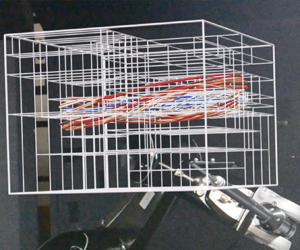
Schematic of the experimental set-up: 1. Computer running COMTree, handling the incoming data stream and sending commands to the robotic manipulator. 2. Data acquisition board. 3. Controller unit of robotic manipulator. 4. Robotic manipulator mounted in the wind tunnel's test section. 5. Multi-hole pressure probe. 6. Vertically mounted NACA 0012 wing. 7.  $5\ \textit {m} \times 3\ \textrm {m} \times 2\ \textrm {m}$ wind tunnel.

Active sampling robotic process and resulting probe path. (a) SmartAIR closed-loop measurement cycle of the processed information and data and (b) probe's path of the model-guided acquisition (cf. Supplementary material and movie).

4.2.2 Results
The measurement domain of  $0.35\ \textrm {m} \times 0.4\ \textrm {m} \times 0.45\ \textrm {m}$ was scanned with the autonomous robotic manipulator for a total of 264 s to reach a largest uncertainty of $0.1$. Figures 9(a) and 9(b) compare two slices of the volumetric measurement data and show the differences in the total pressure coefficients between the moving traverse and the robotic manipulator. The low total pressure and high tangential velocities inside the vortex core are clearly visible in the result from the robotic manipulator. Here, the uncertainty metric of COMTree leads to a denser allocation of measurements in the vortex region (see also Figure 2 with small sub-regions in the vortex region and Figure 8(b) displaying the probe's path) as compared to the traverse with fixed preprogrammed traversing path. In fact, by chance, the preprogrammed traverse did not move through the vortex core's centre, and its reconstruction does not provide a complete picture of the flow field. Remedies such as a rake of probes or denser traversing come with additional costs and intrusiveness or increased traversing times, respectively. At the given flow Reynolds number and angle of attack, the wing experiences leading-edge separation, which can be seen from the low total pressure in the wake at the lower portion of the scalar planes. The two vector fields projected onto the plane show good qualitative agreement in the majority of the field. The largest visible deviation from the COMTree reconstruction is visible in the top left corner, where until the end of the measurement period, the uncertainty metric of COMTree has not yet triggered a refinement of the measurement point pattern (compare with Figure 2 with coarse sub-domains away from the vortex core). Closer to the wingtip, the vortex induces flow attachment, resulting in a mushroom-shaped wake structure, an effect which has been studied e.g. by Reference Zarutskaya and ArieliZarutskaya and Arieli (2005). Figures 9(c) and 9(d) quantitatively compare the results on the mentioned plane 0.23 m downstream of the wing's trailing edge. The experimental results confirm the results derived by the numerical simulation with increased deviation in the turbulent wake. Further, Figure 9( f) compares the traversing techniques along a horizontal line (corresponding to a section travelled by the moving and steady traverse) being normal to the flow direction and cutting through the wing's wake. The turbulent wake of the separated flow is difficult to sample by traversing pressure probes or any measurement method without extensive sampling of individual locations. Figures 9(c), 9(d) and 9( f) underline the two main error sources of the COMTree predictions. First, an insufficient number of iid samples does not fully capture the mean in regions with large fluctuations. Second, cells covering a large area might predict inaccurate mean values due to extrapolation in large parts of the cell (e.g. downward flow field in the top left corner of Figure 9b). This effect is further increased by the application of linear regression submodels. Comparison of COMTree shows good agreement with the IDW interpolation. The latter is expected to fit well with the reference given by the steady traverse, as both share the same path in space. The piecewise constant sections of the COMTree reconstruction reproduce the overall pressure shape well while, at the same time, closely coincide with the averaged pressure values from the steady traverse.
(a,b) Comparison of slices with measured pressure indicated by colour and the planar projection of the velocity vector field by line integral convolution and scaled vectors. (c,d) Normalized errors of the comparison of total pressure and velocity magnitude between the moving traverse and the COMTree reconstruction. (f,g) Comparison of the flow field of the moving with respect to steady traverse and the COMTree reconstruction along a horizontal line normal to the bulk flow. The line corresponds to a straight section of the traverse path as shown by the velocity vectors in panel (g). Black dots indicate the path of the pressure probe within the domain. (a) Moving traverse. Scanning the complete domain of interest in an ordered fashion. (b) The probe guided by the uncertainty metric provided by COMTree. (c) Normalised squared difference  $C_{PT}$ along the moving traverse path. (d) Normalised squared difference velocity magnitude along the moving traverse path. (e) Location of plane in panels (a)–(d). (f) Pressure coefficient and (g) velocity vectors colour-coded with pressure.

Figure 10 provides a quantitative comparison showing the error statistics of the SmartAIR measurement compared to the moving traverse case and the averaged traverse measurement for the total pressure coefficient measurements and each velocity component on a grid aligned with the traverse path. The error of the COMTree prediction compared to the average traversing samples is small. The mean of the error shows excellent agreement, while the standard deviations of the errors are either comparable or larger when compared to the errors of SmartAIR and the moving traverse. This is an expected result as the steady and moving traverse both followed an identical path, while the SmartAIR results, however, incur an interpolation error to these locations.
Box-and-whisker plots of error statistics of the COMTree (CT) predictions compared to the measurements of the moving (Moving T) and steady traverse (Steady T) for the pressure coefficient and the Cartesian velocity components of the flow field. The measurement statistics are calculated from 250 samples for the steady traverse and 52 275 in the case of the moving traverse. A table of exact values and plots of the full outlier range can be found in the Appendix. (a) Error of CT and Steady T, (b) error of CT and Moving T and (c) error of Moving T and Steady T.

The measurement times of the three wind tunnel measurements are listed in Table 1. The speedup in these cases is between a factor of two to five, which we expect to be at the lower end of the system's potential (see also Figure 6). The reference measurements of the moving and steady traverse can potentially take much longer as the number of sampled locations is increased or the probe's traversing speed is decreased to achieve larger data fidelity. The traversing parameters are arbitrary but reflect a sensible choice to keep the reference measurement times small and allow precise three-dimensional flow field reconstructions.
Comparison of measurement times for the conducted experiments and sampling techniques.

5. Conclusion
Flow measurement campaigns, especially in wind tunnels, are often time-critical due to high operating costs. In this work, we have presented a probe-based flow reconstruction framework that is based on a non-parametric regression tree referred to as COMTree. The adapted tree architecture allows for parallel assimilation of newly recorded measurements inducing local refinements in the flow-field reconstruction. The resulting method delivers a reconstruction that is assembled in real-time and that is furthermore accompanied by an uncertainty map. The latter enables a fully autonomous measurement system referred to as SmartAIR, which involves a robotic probe manipulator. Here, the robot takes measurements while moving in-between the inside of regions of maximal uncertainty.
The capabilities of the COMTree method were assessed in a synthetic two-dimensional case with available ground truth and the performance of the complete SmartAIR system was assessed in a three-dimensional wind tunnel test. Our results document that COMTree enables autonomous acquisition as in the SmartAIR system that can deliver locally refined flow measurements in a small fraction of the time required by traditional traverse-based systems. Furthermore, the adaptive character of our approach requires comparatively little prior knowledge about the flow to be investigated.
While the COMTree flow reconstruction incorporates available point measurements, it enforces at the same time continuity of incompressible flows. Further adaptations for compressible flows are conceivable. Moreover, with data points being gathered along the probe path, path planning approaches that take into account the uncertainty metric along the path to the point of maximal uncertainty could be developed as well. To our knowledge, SmartAIR with a robotic manipulator and real-time feedback is the first fully autonomous wind-tunnel flow field measurement system.
Supplementary material and movie
Supplementary material and movie are available at https://doi.org/10.1017/flo.2022.32.
Declaration of interests
The authors declare no conflict of interest.
Funding statement
Funding through the chair of T.R. and from ETH Zürich is gratefully acknowledged.
Author contributions
J.H., D.W.M. and T.R. devised the concept of the presented method. J.H. prepared the data acquisition hardware and driver software, while D.W.M. contributed a single-target-variant of the regression tree applied in this work. F.S. developed, implemented, and tested the outlined physics-constrained multi-target regression tree. F.S. and J.H. conducted the two-dimensional and three-dimensional tests of the method. The article was written by F.S., J.H. and D.W.M. Final edits to the manuscript were made by T.R.
Data availability statement
Data underlying the results presented in this paper are not publicly available at this time but may be obtained from the authors upon reasonable request.
Ethical standards
The research meets all ethical guidelines, including adherence to the legal requirements of the study country.


 Open access