


Impact Statement
Substantial reduction of transport aircraft drag can be achieved by maintaining laminar flow over large portions of the aircraft surfaces, thus enabling a significant reduction of aircraft fuel consumption and polluting emissions. The effectiveness of drag reduction via ‘natural laminar flow’ design of transport aircraft surfaces has been demonstrated in the last decades for surfaces with sweep angles up to approximately 25°, on which amplification of streamwise boundary-layer instabilities is the predominant mechanism leading to laminar–turbulent transition. However, instability amplification may be enhanced by surface imperfections, such as steps and gaps at structural joints, thus inducing premature transition and increased aircraft drag. The present study provides quantitative information and evaluation criteria for the identification of the allowable size of forward-facing steps, which are commensurate with the maintenance of a laminar boundary layer over unswept and moderately swept surfaces of commercial transport aircraft.
1. Introduction
The efforts in commercial aircraft design are currently focusing on the reduction of fuel consumption, emissions and costs (see e.g. Reference CrouchCrouch (2015), Reference Lynde and CampbellLynde and Campbell (2017), Reference Liu, Elham, Horst and HepperleLiu, Elham, Horst, and Hepperle (2018) and references therein). The goals for the reduction in polluting emissions have been concretized by the European Commission as a 75 % cut in CO2 emissions and a 90 % cut in NOx emissions, relative to the capabilities of typical new aircraft in 2000 (European Commission, 2011). Similar targets have been set by NASA (Reference Bezos-O'Connor, Mangelsdorf, Maliska, Washburn and WahlsBezos-O'Connor, Mangelsdorf, Maliska, Washburn, & Wahls, 2011). Part of the goals of emission reduction can be attained by improvements in materials, engines, manufacturing processes, systems optimization and integration, infrastructure, fuel and operational procedures (European Commission, 2011). However, the benefits gained by advances in these disciplines would not be sufficient to reach the emission reduction targets; improvements in the aircraft aerodynamics, and in particular in the reduction of drag, are needed. Skin-friction drag is the major source of drag of commercial transport aircraft, contributing about half of the total aircraft drag (Reference CostantiniCostantini, 2016; Reference JoslinJoslin, 1998). Since the boundary layer on typical transport aircraft is mostly turbulent (Reference BraslowBraslow, 1999), substantial friction drag reduction would be enabled by maintaining laminar flow over large portions of the aircraft surfaces. In fact, at the high Reynolds numbers typical for transport aircraft, the skin-friction coefficient of laminar flow is approximately one order of magnitude lower than that for turbulent flow (Reference JoslinJoslin, 1998). Past research (summarized, e.g., in Reference BraslowBraslow, 1999; Reference JoslinJoslin, 1998) has demonstrated the effectiveness of laminar flow technology for a wide range of aircraft classes, including commercial transport aircraft; nowadays, some components of a few operating commercial airplanes feature laminar flow technology (Reference CrouchCrouch, 2015).
A major concern about the large-scale application of laminar flow technology to commercial transport aircraft is not whether laminar flow can be obtained, but whether this technology can be applied under typical production standards (Reference HansenHansen, 2010). Surface imperfections, such as steps and gaps at structural joints, are very probably unavoidable. They can induce the amplification of existing (or potentially existing) disturbances within the laminar boundary layer and/or the generation of additional instabilities, hence leading to premature transition to turbulence (Reference ArnalArnal, 1992; Reference Holmes, Obara, Martin and DomackHolmes, Obara, Martin, & Domack, 1985; Reference NayfehNayfeh, 1992). Therefore, the essential question is whether laminar flow can be achieved even in the presence of surface imperfections, thus maintaining the related advantages in terms of drag reduction. Manufacturing tolerances must be specified for the shape and dimension of the imperfections so that laminar flow can still be achieved, without, however, being overly stringent.
Criteria to model imperfection effects in the aircraft design and to identify allowable tolerances can be provided only after the influence of the surface imperfections on boundary-layer transition has been understood and quantified. Previous studies have considered surface discontinuities in the form of forward-facing steps, backward-facing steps and gaps. This work focuses on sharp, two-dimensional (i.e. spanwise-invariant) forward-facing steps, placed on an aerodynamic surface perpendicular to a (quasi-) two-dimensional flow. Gaps have been studied in Reference Nenni and GluyasNenni and Gluyas (1966), Reference Zahn and RistZahn and Rist (2016, Reference Zahn and Rist2017), Reference Beguet, Perraud, Forte and BrazierBeguet, Perraud, Forte, and Brazier (2017), Reference Dimond, Costantini, Risius, Fuchs and KleinDimond, Costantini, Risius, Fuchs, and Klein (2019), Reference Dimond, Costantini, Risius, Klein and ReinDimond, Costantini, Risius, Klein, and Rein (2020) and Reference Crouch, Kosorygin and SutantoCrouch, Kosorygin, and Sutanto (2020), among others, while backward-facing steps have been also considered in part of the publications discussed below with regard to forward-facing steps. Combinations of forward- and backward-facing steps in the form of rectangular protrusions or wide gaps have been examined, e.g. in Reference Crouch and KosoryginCrouch and Kosorygin (2020), Reference Franco Sumariva, Hein and ValeroFranco Sumariva, Hein, and Valero (2020) and Reference Tocci, Franco, Hein, Chauvat and HanifiTocci, Franco, Hein, Chauvat, and Hanifi (2021); combinations of forward-facing steps and gaps have been studied in Reference Zahn and RistZahn and Rist (2017) and Reference Dimond, Costantini, Risius, Fuchs and KleinDimond et al. (2019, Reference Dimond, Costantini, Risius, Klein and Rein2020), focusing on the transition delay by means of wall suction. Wall suction has been also considered in Reference Zhao and DongZhao and Dong (2020) and Reference Lüdeke and von SoldenhoffLüdeke and von Soldenhoff (2021) to delay step-induced transition. The effect of steps on swept-wing transition induced by predominant cross-flow instabilities has been investigated, e.g. in Reference Perraud and SeraudiePerraud and Seraudie (2000), Reference Duncan, Crawford, Tufts, Saric and ReedDuncan, Crawford, Tufts, Saric, and Reed (2014), Reference Tufts, Reed, Crawford, Duncan and SaricTufts, Reed, Crawford, Duncan, and Saric (2017), Reference EppinkEppink (2018) and Reference Rius-Vidales and KotsonisRius-Vidales and Kotsonis (2020, Reference Rius-Vidales and Kotsonis2021). The influence of the imperfection shape on step-induced transition has been studied in Reference Holmes, Obara, Martin and DomackHolmes et al. (1985) and Reference Zahn and RistZahn and Rist (2017) by examining steps with rounded corners.
Most of the previous experimental and numerical studies on two-dimensional step effects have focused on incompressible flat-plate flows, mainly at zero pressure gradient (Reference Crouch and KosoryginCrouch & Kosorygin, 2020; Reference Crouch, Kosorygin and NgCrouch, Kosorygin, & Ng, 2006; Reference Drake, Bender, Korntheuer, Westphal, McKeon, Gerashchenko and DaleDrake et al., 2010; Reference Lin and WangLin & Wang, 2021; Reference Nenni and GluyasNenni & Gluyas, 1966; Reference Perraud and SeraudiePerraud & Seraudie, 2000; Reference Rizzetta and VisbalRizzetta & Visbal, 2014; Reference Tocci, Franco, Hein, Chauvat and HanifiTocci et al., 2021; Reference Wang and GasterWang & Gaster, 2005). These studies have provided valuable information on the influence of two-dimensional steps on the stability and transition of (quasi-) two-dimensional boundary layers in a low disturbance environment, in which the amplification of Tollmien–Schlichting (TS) waves is the predominant instability mechanism leading the boundary layer to transition (Reference ArnalArnal, 1992; Reference Crouch and KosoryginCrouch & Kosorygin, 2020; Reference SchraufSchrauf, 2005). The effect of the streamwise pressure gradient on step-induced transition at low speed has been examined in Reference Perraud and SeraudiePerraud and Seraudie (2000), Reference Crouch, Kosorygin and NgCrouch et al. (2006), Reference Drake, Bender, Korntheuer, Westphal, McKeon, Gerashchenko and DaleDrake et al. (2010) and Reference Crouch and KosoryginCrouch and Kosorygin (2020).
The influence of steps on transition of an airfoil boundary layer has been studied at subsonic speeds (Mach numbers  $M = U_\infty /a_\infty \le 0.35$, where U∞ and a∞ are the free-stream velocity and speed of sound, respectively) in Reference Perraud and SeraudiePerraud and Seraudie (2000) and Reference Costantini, Risius, Klein and KühnCostantini, Risius, Klein, and Kühn (2016b).
A compressible boundary layer over a flat plate has been examined in Reference Edelmann and RistEdelmann and Rist (2014, Reference Edelmann and Rist2015) at Mach numbers up to M = 1.06, whereas the flight tests analysed in Reference SchraufSchrauf (2018) have been conducted at M = 0.75 and 0.8 using a natural laminar flow (NLF) glove.
The above literature overview clearly shows that earlier work on step-induced transition has mainly considered flat-plate configurations at low speed. In particular, experiments have been conducted at Mach numbers M ≤ 0.35 and unit Reynolds numbers  $R{e}^{\prime} = U_\infty /\nu _\infty < 6\,\cdot \,10^6\;{\rm m}^{{-}1}$ (where ν∞ is the free-stream kinematic viscosity), except for the few cases analysed in Reference SchraufSchrauf (2018). Some of the previous studies have examined the influence of the streamwise pressure gradient, but in these cases the pressure distribution in the streamwise direction has been generally not uniform: in particular, the pressure gradients at the step location and at the transition location have been different.
A systematic study of the effect of forward-facing steps on boundary-layer transition is carried out in the present work, in which the influence of changes in Mach number, Reynolds number and streamwise pressure gradient is also investigated. The experiments have been conducted in a quasi-two-dimensional flow at unit Reynolds numbers up to  $R{e}^{\prime} = 65\,\cdot \,10^6\;{\rm m}^{{-}1}$ and at Mach numbers up to M = 0.77. The adopted experimental set-up, based on a flat-plate configuration (Reference Costantini, Hein, Henne, Klein, Koch, Schojda and SchröderCostantini et al., 2016a), allows an independent variation of the aforementioned parameters; hence, it enables a decoupling of their respective effects on the boundary-layer transition, which has been detected accurately and non-intrusively by means of a temperature-sensitive paint (TSP). The experimental set-up is briefly described in § 2. The experimental data measured for the smooth (no step) configuration serve also as inputs for laminar boundary-layer computations, which are conducted to obtain velocity and temperature profiles. The boundary-layer profiles are analysed according to compressible, linear, local stability theory (see Reference ArnalArnal (1992), among others) to determine the amplification factors (N-factors) of TS waves. The numerical procedure is summarized in § 3. The present work is built on and extends the studies with the same experimental set-up presented in previous publications (Reference Costantini, Hein, Henne, Klein, Koch, Schojda and SchröderCostantini et al., 2016a, Reference Costantini, Risius, Klein and Kühn2016b; Reference Costantini, Risius and KleinCostantini, Risius, & Klein, 2015a, Reference Costantini, Risius and Klein2018a), and is based on Reference CostantiniCostantini (2016) and Reference Costantini, Risius and KleinCostantini, Risius, and Klein (2018b). The elements of novelty of the current work are summarized below.
• As compared with the earlier publications, in which the Mach numbers M = 0.35 and 0.77 have been examined, two additional Mach numbers (M = 0.50 and 0.65) are considered here. The examined conditions are reported in § 4.
• The results at all four Mach numbers are analysed to determine functional relations for the design of NLF surfaces at zero to moderate sweep angles. Proposals for criteria to identify allowable step heights for NLF surfaces at the investigated flow conditions are derived from these functional relations and presented in § 5.
• Following the procedure described in Reference Wang and GasterWang and Gaster (2005), Reference Crouch, Kosorygin and NgCrouch et al. (2006) and Reference Crouch and KosoryginCrouch and Kosorygin (2020), the N-factor distributions obtained with the smooth configuration are correlated with the transition locations measured in the experiments with smooth and step configurations, thus providing the step-induced increment in the transition N-factor ΔN. The values of ΔN determined for the range of examined test conditions are presented and discussed in § 6 with regard to those reported in the literature. The results support a modelling of the step effect on boundary-layer transition in the established eN method for transition prediction on NLF surfaces.
2. Experimental set-up
The tested model is the PaLASTra two-dimensional flat-plate configuration (explained and defined in Reference CostantiniCostantini, 2016; Reference Costantini, Hein, Henne, Klein, Koch, Schojda and SchröderCostantini et al., 2016a). As shown in figure 1(a), it features a flat surface for the largest part of the model upper side, which is the surface of major interest in this study. It has been designed to achieve an essentially uniform streamwise pressure gradient in the region at approximately 20 % < x/c < 70 %; this enables a decoupling, and thus a systematic study, of the effects on boundary-layer transition of various contributing factors, such as the height of forward-facing steps, the Mach and Reynolds numbers and the pressure gradient itself. The wind-tunnel model has been also designed to provide sharp steps of variable height on the surface of interest. Two-dimensional forward-facing steps of different height h are generated on the model upper surface at xh/c = 35 %, perpendicular to the free-stream direction and normal to the surface (see figure 1).
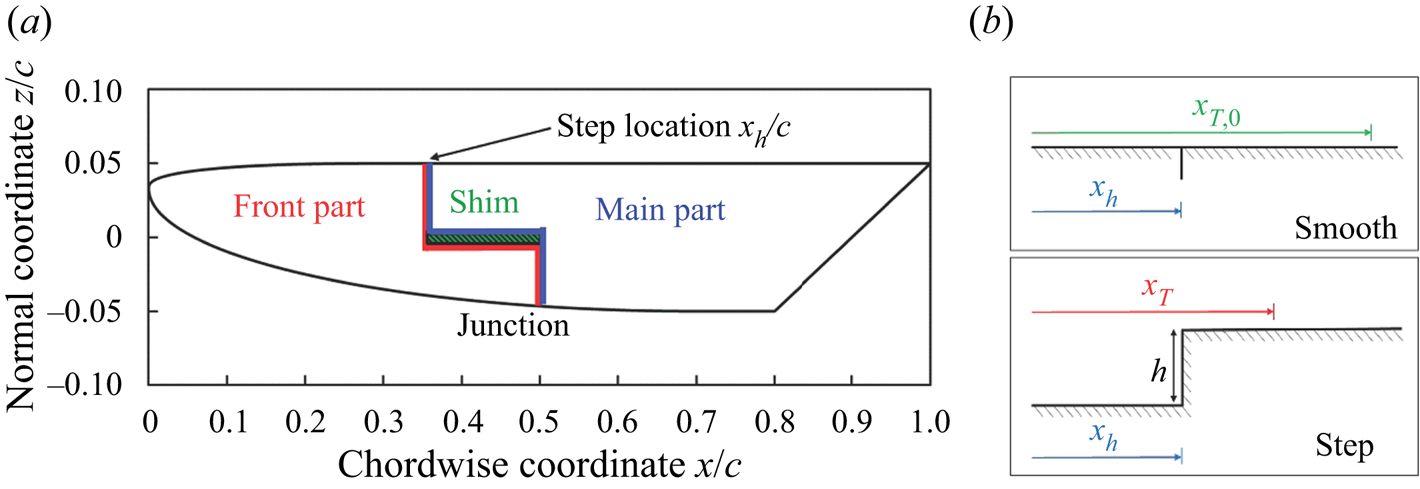
Figure 1. (a) Simplified drawing of the PaLASTra model construction (side view, Reference CostantiniCostantini, 2016); (b) schematic representation of the smooth and step configurations with the corresponding transition locations: xT ,0 and xT.
Global, non-intrusive measurements of boundary-layer transition have been carried out by means of a TSP (Reference Ondrus, Meier, Klein, Henne, Schäferling and BeifussOndrus et al., 2015). When excited by light at a wavelength of approximately 405 nm, the used TSP emits light at approximately 615 nm, the intensity of which decreases at larger temperatures. The distribution of light emitted by the TSP has been captured by means of two cameras, thus enabling the global detection of the temperature variation between the laminar and turbulent flow regions, and therefore of the boundary-layer transition (see § 4). The TSP has been applied in pockets machined into the model upper surface. Since the TSP completely fills the pockets, the final model contour corresponds to the designed one. With this model design, the sharpness of the step is ensured (Reference CostantiniCostantini, 2016; Reference Costantini, Risius and KleinCostantini et al., 2018a). The model is also equipped with a row of pressure taps for the measurement of the surface pressure distribution, which is analysed to determine a pressure gradient parameter (see § 4) and also serves as input for boundary-layer computations, such as those described in § 3.
The experiments have been conducted in the Cryogenic Ludwieg-Tube Göttingen (KRG) (Reference KochKoch, 2004; Reference RosemannRosemann, 1997), which is a Ludwieg-tube facility using nitrogen as test gas. Reynolds and Mach numbers relevant for commercial transport aircraft can be achieved at KRG in spite of the small chord length of the two-dimensional models typically investigated in this facility (c ≤ 0.2 m). This is accomplished by increasing the pressure and decreasing the temperature of gaseous nitrogen. The adaptive upper and lower walls of the 0.4 m wide, 0.35 m high and 2 m long test section allow interference-free contours to be set. As reported in Reference KochKoch (2004), KRG has good flow quality; for example, the turbulence level determined from the momentum fluctuations is Tuρu ~ 0.06 % in the frequency bandwidth 10 Hz–10 kHz. These characteristics make KRG an appropriate facility for NLF testing at high Reynolds numbers and at both subsonic and transonic Mach numbers. A further aspect that should be considered for experiments in KRG is related to the working principle of this Ludwieg-tube facility: the temperature difference between flow and model surface occurs during a test run because of the expansion process of the gas flow. This temperature difference enables very accurate transition measurements, since the temperature difference between flow and model surface enhances the surface temperature difference between laminar and turbulent flow regions, which is detected via TSP (Reference Costantini, Fey, Henne and KleinCostantini, Fey, Henne, & Klein, 2015b; Reference Costantini, Hein, Henne, Klein, Koch, Schojda and SchröderCostantini et al., 2016a). However, the resulting non-adiabatic surface (wall temperature ratio Tw/Taw > 1, where Tw and Taw are the model surface temperature and the adiabatic-wall temperature, respectively) also influences boundary-layer stability and transition (Reference ArnalArnal, 1992; Reference Costantini, Fey, Henne and KleinCostantini et al., 2015b, Reference Costantini, Hein, Henne, Klein, Koch, Schojda and Schröder2016a; Reference Costantini, Risius and KleinCostantini, Risius, & Klein, 2020). The effect of the wall temperature ratio on step-induced boundary-layer transition has been investigated in Reference CostantiniCostantini (2016) and Reference Costantini, Risius and KleinCostantini et al. (2018a).
In summary, the experimental set-up is suited for the systematic investigation of the influence of sharp forward-facing steps on boundary-layer transition at test conditions relevant for unswept and moderately swept aerodynamic surfaces of commercial transport aircraft, for which TS waves are the predominant instability mechanism leading to transition. Details on the experimental set-up and on its accuracy are given in Reference Costantini, Hein, Henne, Klein, Koch, Schojda and SchröderCostantini et al. (2016a), Reference CostantiniCostantini (2016) and Reference Costantini, Risius and KleinCostantini et al. (2018a).
3. Numerical procedure and correlation with experimental data
An established method for transition prediction is the so-called ‘eN method’, which is based on linear, local stability theory (see § 1). In the present case of a quasi-two-dimensional flow, the N-factor (N) is the amplification factor of TS waves. The eN method assumes that transition occurs at the location where a threshold amplification factor is reached by the N-factor envelope curve, which is the curve connecting the maxima of N for all amplified TS waves at each streamwise location. This transition prediction method therefore considers only the linear amplification of primary modes (here, the TS waves). All other physics, receptivity and nonlinear breakdown included, are incorporated into the threshold N-factor, which is calibrated by means of experimental data. The free-stream parameters and the surface pressure distributions measured on the smooth configuration are used to conduct laminar boundary-layer computations by means of the boundary-layer solver COCO (Reference SchraufSchrauf, 1998), with consideration of the examined non-adiabatic surface (Reference CostantiniCostantini, 2016; Reference Costantini, Hein, Henne, Klein, Koch, Schojda and SchröderCostantini et al., 2016a, Reference Costantini, Risius and Klein2020). The calculated wall-normal velocity and temperature profiles are analysed by means of the stability analysis tool LILO (Reference SchraufSchrauf, 2006) to obtain the N-factors of TS waves with different frequencies, according to compressible, linear, local stability theory. Only two-dimensional TS waves are considered in this work, since the Mach number at the boundary-layer edge remains subsonic at all examined test conditions (Reference Costantini, Hein, Henne, Klein, Koch, Schojda and SchröderCostantini et al., 2016a). The N-factor envelope curves are then correlated with the measured transition locations (xT and xT ,0, see figure 1b) to determine the transition N-factors, i.e. the maximal N-factors at the transition location:  $N_T = N_{max}(x_T)$ and $N_{T,0} = N_{max}(x_{T,0})$. It should be noted here that the N-factor envelope curves N(x) calculated for the smooth configuration are used in this work to determine both NT and NT ,0 (see § 6), following the procedure discussed in Reference Wang and GasterWang and Gaster (2005) and Reference Crouch, Kosorygin and NgCrouch et al. (2006). For the present experimental set-up in KRG, the average transition N-factor for the smooth configuration varies in the range NT ,0 = 5.3–7.6, depending on the free-stream Mach number. The scatter in the determined values of NT ,0 is within approximately ±25 % about the corresponding averages (Reference Costantini, Hein, Henne, Klein, Koch, Schojda and SchröderCostantini et al., 2016a, Reference Costantini, Risius and Klein2020). These moderate values of transition N-factor are likely due to acoustic disturbances originating from the large separated flow region downstream of the model aft side (see figure 1a) and travelling upstream, as discussed in Reference CostantiniCostantini (2016) and Reference Risius, Costantini, Koch, Hein and KleinRisius, Costantini, Koch, Hein, and Klein (2018).
4. Examined conditions
The experiments have been conducted at Mach numbers M = U∞/a∞ = 0.35 to 0.77 and chord Reynolds numbers  $Re = U_\infty c/\nu _\infty = 4$ to 13 ⋅ 106 for various step heights and streamwise pressure gradients. The range of examined parameters is summarized in table 1. For the description of the streamwise pressure gradient, a single, characteristic parameter is evaluated from the nearly uniform surface pressure distributions measured by means of the pressure taps. In the present study, the Hartree parameter βH of the self-similar solution of the boundary-layer equations (Falkner–Skan equation) (Reference Meyer and KleiserMeyer & Kleiser, 1989) is chosen as pressure gradient parameter. As discussed in Reference Risius, Costantini, Koch, Hein and KleinRisius et al. (2018), the Hartree parameter has a relationship with other parameters characterizing the streamwise pressure gradient, such as the boundary-layer shape factor.
Table 1. Variation of the examined parameters.

Mainly favourable pressure gradients (βH > 0) are examined in the present work (see table 1), since they are the most relevant for NLF surfaces. Nevertheless, also nearly zero (βH ~ 0) and adverse pressure gradients (βH < 0) are considered. Four surface pressure distributions measured at M = 0.77 and Re = 6 ⋅ 106 are exemplarily shown in figure 2(a). They correspond to a nearly zero pressure gradient (βH = 0.005) and three favourable pressure gradients with different levels of flow acceleration. The N-factor envelope curves calculated on the basis of these pressure distributions are shown in figure 2(b). These N-factor results have been discussed in detail in Reference Costantini, Hein, Henne, Klein, Koch, Schojda and SchröderCostantini et al. (2016a).

Figure 2. Surface pressure distributions measured at M = 0.77 and Re = 6 ⋅ 106 for different Hartree parameters (a) and corresponding N-factor envelope curves (b). Transition measured at xT/c = 36.3 ± 0.3 % (βH = 0.005), xT/c = 44.4 ± 0.3 % (βH = 0.036), xT/c = 55.4 ± 0.5 % (βH = 0.051) and xT/c = 69.2 ± 1.0 % (βH = 0.063).
Surface pressure distributions measured at M = 0.77, Re = 6 ⋅ 106 and βH = 0.063 for the different model configurations are presented in figure 3. As can be seen in figure 3(a), the steps do not affect the pressure distributions globally, but induce significant pressure gradients in the vicinity of the steps (see zoomed-in plots in figure 3b): the larger the step, the larger is the difference of the pressure distribution compared with that on the smooth configuration. Because of these local step-induced pressure gradients, the Hartree parameter for the step configurations is not evaluated from the actual surface pressure distributions; in fact, the agreement of the pressure distributions on the remaining areas allows the approximation of an unchanged global Hartree parameter. Thus, the Hartree parameter for the step configurations is assumed to be the same as that of the corresponding smooth configuration.

Figure 3. Surface pressure distributions with different model configurations at Re = 6 ⋅ 106, M = 0.77 and βH = 0.063. Smooth: h = 0  $\mu$m; step-1: h = 29 $\mu$m; step-2: h = 60 $\mu$m; step-3: h = 89 $\mu$m. (a) Over the whole chord length; (b) zoomed-in around the step location. The grey bar indicates the step location.
The values of Mach number, Reynolds number and Hartree parameter in the experimental investigation have been well repeatable and reproducible. As mentioned in § 2, the working principle of KRG leads to a non-adiabatic surface. The wall temperature ratio increases at larger Mach numbers (see table 1) and cannot be set at a particular value with an accuracy comparable to that of the other parameters. This is due to the sensitivity of Tw/Taw to even small variations of the temperatures of the model surface and/or of the gas in the KRG storage tube between the test runs (Reference CostantiniCostantini, 2016; Reference Costantini, Risius and KleinCostantini et al., 2018a, Reference Costantini, Risius and Klein2020). For this reason, a range of Tw/Taw is reported in table 1 for each examined Mach number, i.e. it covers the values of Tw/Taw for all experiments conducted at a certain Mach number. It should, however, be noted here that the uncertainty in the wall temperature ratio for a single test run is within  $\varDelta (T_w/T_{aw}) = {\pm} 0.002$ (Reference Costantini, Hein, Henne, Klein, Koch, Schojda and SchröderCostantini et al., 2016a).
Boundary-layer transition is determined from the TSP data according to the methodology described in Reference CostantiniCostantini (2016) and Reference Costantini, Henne, Risius and KleinCostantini, Henne, Risius, and Klein (2021). The distributions of the TSP luminescent intensity (and therefore of the surface temperature) captured by the two cameras are mapped onto a three-dimensional grid representing the model upper surface, and then analysed by means of a robust algorithm capable of reliably and automatically detecting the maximal streamwise temperature gradient in the transitional region. This location is defined as ‘the’ transition location xT/c in the present work. This choice is motivated and substantiated by earlier work, and the methodology has been also validated against transition data obtained using uncorrelated transition detection methods: the established σcp method, which is based on the measurement of surface pressure fluctuations, and the global luminescent oil-film skin-friction field estimation method, which provides skin-friction distributions (Reference Costantini, Henne, Risius and KleinCostantini et al., 2021). The capability to detect a single, well-defined, accurately and consistently measurable transition location is essential for the systematic analysis of the effect of different factors on boundary-layer transition, as conducted in the current study. The uncertainty in the measured transition location is within  $\varDelta (x_T/c) = {\pm} 2\,\%$ (less than $\varDelta (x_T/c) = {\pm} 1\,\%$ for the majority of the cases). The main contribution to $\varDelta (x_T/c)$ is due to the spanwise variation of the transition location (Reference CostantiniCostantini, 2016).
Details on the evaluation of the aforementioned parameters, on their repeatability, reproducibility and uncertainty, as well as on the data acquisition and post-processing, are given in Reference Costantini, Hein, Henne, Klein, Koch, Schojda and SchröderCostantini et al. (2016a) and Reference CostantiniCostantini (2016).
5. Analysis of the experimental results
The transition results have been thoroughly discussed in previous publications (Reference CostantiniCostantini, 2016; Reference Costantini, Risius and KleinCostantini et al., 2015a, Reference Costantini, Hein, Henne, Klein, Koch, Schojda and Schröder2016a, Reference Costantini, Risius, Klein and Kühn2016b, Reference Costantini, Risius and Klein2018a, Reference Costantini, Risius and Klein2020). A main focus of the present work is on the identification of functional relations that represent the effect of forward-facing steps on boundary-layer transition at various subsonic Mach numbers. A quantitative description of the evolution of the transition location, as induced by a variation of the examined parameters, is supported by dimensional analysis of the variables involved in the problem (Reference CostantiniCostantini, 2016; Reference DrydenDryden, 1953). For the present problem, the functional relations between the dimensional quantities can be reduced to general relations between two independent non-dimensional parameters: a non-dimensional roughness parameter, and a non-dimensional parameter representing the step-induced variation of the transition location with respect to the smooth configuration. Three non-dimensional roughness parameters, which have been considered in earlier publications, are used in the present analysis: the step Reynolds number  $Re_h = U_\infty h/\nu _\infty $ (Reference Nenni and GluyasNenni & Gluyas, 1966; Reference Perraud and SeraudiePerraud & Seraudie, 2000), the relative step height $h/\delta _{1,h} = h/\delta _1(x_h)$ (Reference Crouch, Kosorygin and NgCrouch et al., 2006; Reference Perraud and SeraudiePerraud & Seraudie, 2000; Reference Wang and GasterWang & Gaster, 2005) and the roughness Reynolds number $Re_k = U_hh/\nu _h = U(x_h)h/\nu (x_h)$ (Reference Drake, Bender, Korntheuer, Westphal, McKeon, Gerashchenko and DaleDrake et al., 2010; Reference Rizzetta and VisbalRizzetta & Visbal, 2014). Here, the boundary-layer displacement thickness δ 1,h is evaluated at the step location xh in the undisturbed laminar boundary layer (no step present); similarly, the streamwise mean-velocity component Uh and the kinematic viscosity νh for Rek are those that would be found at x = xh and z = h for the smooth surface. The quantities δ 1,h, Uh and νh are evaluated from the results of the boundary-layer computations conducted for the smooth configuration (see § 3). The non-dimensional parameter representing the step-induced variation of the transition location is $s = (x_T-x_h)/(x_{T,0}-x_h)$, where xT and xT ,0 are the transition locations measured with and without steps, respectively (see figure 1b). The value of this characteristic parameter is s = 1 when transition is unaffected by the step, whereas it goes to zero when the transition location approaches the step location. The parameter s has been already used in previous studies (Reference Duncan, Crawford, Tufts, Saric and ReedDuncan et al., 2014; Reference Perraud and SeraudiePerraud & Seraudie, 2000) and allows the step-induced variation of the transition location to be ‘isolated’, since it represents the relative change in transition location with respect to the step location (Reference CostantiniCostantini, 2016), and thus considers only the region over which the boundary layer develops after it has undergone amplification in the step area.
All experimental data obtained at the four examined Mach numbers are collected in three single plots in figure 4; s is presented as a function of Reh, h/δ 1,h and Rek in figures 4(a)–4(c), respectively. The data obtained at different Mach numbers are shown by symbols with different colours. The coloured lines show the approximation functions for the data obtained at the corresponding Mach numbers (i.e. for the data points with the same colour). These functions are identified as those that are best matched by the experimental data in the least-squares sense, with the vertical axis intercept forced to s = 1. A curve approximating the whole set of data is also shown in each plot by a thick black line. These approximation functions are determined in the same manner as those for the data sets at different Mach numbers. Note that the horizontal axis in figure 4(c) has a logarithmic scale to highlight the results obtained at low values of roughness Reynolds number. It should be also remarked that Reh and h/δ 1,h are linear functions of the roughness height h, whereas the dependence of Rek is essentially quadratic (Reference DrydenDryden, 1953), thus suggesting a difference in the dependency of s on the non-dimensional step parameters. The three functional plots give a good correlation of the results, clearly showing that  $s = (x_T-x_h)/(x_{T,0}-x_h)$ decreases gradually at larger values of Reh, h/δ 1,h and Rek. As discussed in previous work for M = 0.35 (Reference Costantini, Risius, Klein and KühnCostantini et al., 2016b) and 0.77 (Reference Costantini, Risius and KleinCostantini et al., 2015a, Reference Costantini, Risius and Klein2018a), the correlations are essentially independent of chord Reynolds number and streamwise pressure gradient. This finding is confirmed also for the two intermediate Mach numbers M = 0.50 and 0.65. For this reason, the data points obtained at a certain Mach number but at different βH and Re are not further distinguished in figure 4 by using different symbols. In addition to the findings related to the chord Reynolds number and the streamwise pressure gradient, figure 4 also shows that the functional relations between s and the non-dimensional step parameters are essentially independent of the Mach number (at least up to intermediate values of the non-dimensional step parameters and in the examined range of M). Besides the Mach number itself, the results obtained at the four different Mach numbers differ also in their disturbance environment, boundary-layer receptivity and thermal condition at the model surface. Nevertheless, at fixed Mach number, Reynolds number and model angle of attack (i.e. streamwise pressure gradient), the wall temperature ratio is approximately the same, and the level and spectrum of the external disturbances (as well as boundary-layer receptivity to such disturbances) are expected to remain unchanged. Thus, the transition locations xT and xT ,0 are measured under almost the same conditions. The use of $s = (x_T-x_h)/(x_{T,0}-x_h)$ as the parameter to describe the change in transition location is confirmed to allow the ‘isolation’ of the step effect on boundary-layer transition, since the influence of the other factors is minimized. Particular aspects to be considered concerning the effect of the wall temperature ratio are discussed in Reference Costantini, Risius and KleinCostantini et al. (2018a). In fact, the deviations of some experimental data from the overall trends presented in figure 4 are mainly due to different wall temperature ratios between the tests with smooth and step configurations.

Figure 4. Relative change in transition location as a function of the step Reynolds number (a), relative step height (b) and roughness Reynolds number (c) for the four examined Mach numbers. Coloured lines show the functions approximating the data at the corresponding Mach numbers, while the thick black lines show the functions approximating the whole set of data.
In summary, the effects of the various factors influencing boundary-layer transition are included in xT and xT ,0, and thereby accounted for when  $s = (x_T-x_h)/(x_{T,0}-x_h)$ is used to describe the shift in transition location due to the steps. The results obtained for the examined PaLASTra model have been already shown to be in agreement with those obtained for an NLF airfoil model (Reference Costantini, Risius, Klein and KühnCostantini et al., 2016b), demonstrating the applicability and transferability of the present results obtained with a generic configuration (flat plate) to the practical case of an NLF airfoil. Criteria for allowable tolerances for forward-facing steps on unswept and moderately swept NLF surfaces can now be derived from the functional relations presented in figure 4. For this scope, the equations of the approximation curves shown by thick black lines in figure 4 are reported below
 $$\begin{gather}s = \displaystyle{{x_T-x_h} \over {x_{T,0}-x_h}} = a\cdot e^{(-{(b-Re_h)}^2/2\cdot c^2)},\end{gather}$$
for figure 4(a), with a = 1.016, b = −326, and c = 1995;
 $$\begin{gather} s = \displaystyle{{x_T-x_h} \over {x_{T,0}-x_h}} = p\cdot e^{(-{(q-h/\delta _{1,h})}^2/2\cdot r^2)},\end{gather}$$
for figure 4(b), with p = 1.0005, q = 0.007, and r = 0.6; and
 $$\begin{gather} s = 3.4\,\cdot \,10^{{-}14}Re_k^4 -2.6\,\cdot \,10^{{-}10}Re_k^3 + 7.1\,\cdot \,10^{{-}7}Re_k^2 -1.1\,\cdot \,10^{{-}3}Re_k + 1,\end{gather}$$
for figure 4(c). It should be remarked here that (5.1)–(5.3) do not represent well the behaviour of boundary-layer transition at very large values of the non-dimensional step parameters, i.e. at approximately Reh > 4000, h/δ 1,h > 1.3 and Rek > 2500. In these cases, however, transition occurs at a location very close to that of the step, so that the transition location can be approximated by the step location for practical purposes.
At this point, it should be emphasized that the criterion used to define the ‘critical’ step height (subscript ‘cr’) is crucial. Differently from three-dimensional roughness elements (Reference ArnalArnal, 1992; Reference BraslowBraslow, 1999; Reference NayfehNayfeh, 1992), boundary-layer transition in the presence of two-dimensional roughness does not move upstream very rapidly as a critical roughness height is exceeded: this is confirmed in figure 4 for forward-facing steps. Rather, the critical value of a non-dimensional step parameter should be that for which transition has moved by a certain extent from its smooth-configuration location towards the step location. The critical values of Reh, h/δ 1,h and Rek, corresponding to a certain loss of laminarity  $\varDelta s = [1-(x_T-x_h)/(x_{T,0}-x_h)]$ are evaluated from (5.1)–(5.3) and reported in table 2. These values can be used as a guide for manufacturing tolerances of NLF surfaces (with zero to moderate sweep angles) at different flow conditions and streamwise pressure gradients, at least for the examined range of test parameters. The reader is referred to Reference CostantiniCostantini (2016) for a detailed discussion of the evolution of step-induced transition and of the identified critical values of the non-dimensional step parameters, as compared with the findings reported in the literature.

6. Increase in amplification factors (ΔN) due to forward-facing steps
A method to account for the effect of steps in the eN method has been presented in Reference Wang and GasterWang and Gaster (2005) and Reference Crouch, Kosorygin and NgCrouch et al. (2006). The amplification of TS waves due to the presence of the steps is modelled by the increment function ΔN(x), which is to be added to the N-factor envelope curve computed for the smooth configuration. The increment function varies, in general, with the streamwise coordinate (Reference Edelmann and RistEdelmann & Rist, 2014, Reference Edelmann and Rist2015; Reference Perraud and SeraudiePerraud & Seraudie, 2000). In some cases, however, the effect of the imperfection on the N-factor envelope curve vanishes at a location so far downstream of the step location that the increment function can be approximated by a uniform offset ΔN for a considerable streamwise distance. This has been the strategy pursued in Reference Wang and GasterWang and Gaster (2005), Reference Crouch, Kosorygin and NgCrouch et al. (2006) and Reference Crouch and KosoryginCrouch and Kosorygin (2020), where ΔN has been determined from the correlation of the transition locations xT and xT ,0 (measured with and without steps, respectively) with the N-factor envelope curve N(x) obtained for the smooth configuration. In practice, the value of the uniform offset has been determined as  $\varDelta N = N_{T,0}-N_T$. This procedure assumes that receptivity at the step can be neglected, and that the N-factors of the TS waves are increased by the same ΔN. Note that there exists experimental verification that amplified TS waves, predicted by linear stability theory for the smooth surface, are responsible for transition even in the presence of surface steps of considerable relative height (Reference Crouch, Kosorygin and NgCrouch et al., 2006; Reference Wang and GasterWang & Gaster, 2005). Moreover, when transition occurs at a location sufficiently downstream of the step location, the frequency band of the most amplified disturbances has been found to be unchanged for both configurations, with and without steps (Reference Crouch and KosoryginCrouch & Kosorygin, 2020; Reference Crouch, Kosorygin and NgCrouch et al., 2006).
The procedure described in Reference Wang and GasterWang and Gaster (2005) and Reference Crouch, Kosorygin and NgCrouch et al. (2006) to determine the (uniform) increment ΔN is applied also to the present data. The N-factor envelope curves calculated for the smooth configuration are correlated with the measured transition locations with and without steps, in order to obtain the transition N-factors NT ,0 and NT (see § 3) and thus the step-induced increment ΔN. The results are plotted as ΔN vs. h/δ 1,h in figure 5, where the panels show the results obtained at the four different Mach numbers. Among the non-dimensional step parameters, the relative step height h/δ 1,h is selected for the presentation of the results for consistency with the literature. In figure 5, different symbols are used to differentiate the data points at different pressure gradients, in order to examine a possible influence of βH on the correlations. The approximation functions from Reference Wang and GasterWang and Gaster (2005) and Reference Crouch, Kosorygin and NgCrouch et al. (2006) are shown in the figures by solid and dashed lines, respectively. The present data show some scatter, which is, however, still less than that observed in Reference Crouch, Kosorygin and NgCrouch et al. (2006) for a favourable streamwise pressure gradient. A general trend can be seen in figure 5: ΔN increases with larger h/δ 1,h. The experimental data can be fitted using second-order polynomial functions, shown by the dash-dotted lines in the figures. These functions have a shape similar to the curve used to fit the data in Reference Wang and GasterWang and Gaster (2005) in the considered range 0 ≤ h/δ 1,h ≤ 1.6. The fitted function from Reference Crouch, Kosorygin and NgCrouch et al. (2006) seems to represent an upper bound for the present data, a result similar to that obtained in that work for a favourable pressure gradient. (There are only a few data points in figure 5(c,d) that are above this curve, i.e. those at h/δ 1,h > 0.9.) As suggested in Reference Crouch and KosoryginCrouch and Kosorygin (2020), this may be due to the relatively small growth factor of TS waves between xh and xT ,0 observed in the current work (see example in figure 2b). On the other hand, the approximation function from Reference Wang and GasterWang and Gaster (2005) seems to represent a lower bound for the present data. With decreasing Mach number, the slope of the current fitted functions (dash-dotted lines) and, in general, the value of the increment ΔN at fixed h/δ 1,h increase. This result appears to be due to the damping influence of compressibility on ΔN, in agreement with the results obtained in Reference Edelmann and RistEdelmann and Rist (2014) for Mach numbers M = 0.15 and 0.8. The streamwise pressure gradient has no clear effect on the relation between ΔN and h/δ 1,h.

Figure 5. Uniform step-induced increment of amplification factors ΔN as a function of the relative step height for different Mach numbers: (a) M = 0.77; (b) M = 0.65; (c): M = 0.50; (d): M = 0.35. Dash-dotted lines: second-order polynomial functions  $\varDelta N = p_N(h/\delta _{1,h})^2 + q_N(h/\delta _{1,h})$ fitted to the present data, with coefficients: pN = 0.768, qN = −0.058 (a); pN = 0.890, qN = 0.008 (b); pN = 1.042, qN = 0.106 (c); pN = 1.239, qN = −0.085 (d). Solid and dashed lines: fitted functions from Reference Wang and GasterWang and Gaster (2005) and Reference Crouch, Kosorygin and NgCrouch et al. (2006), respectively.
7. Conclusions and final remarks
A systematic study has been carried out in the present work to evaluate the influence of sharp, two-dimensional forward-facing steps on laminar–turbulent transition of a quasi-two-dimensional boundary layer. The flow conditions are relevant for NLF surfaces of commercial transport aircraft. The experiments have been conducted at Mach numbers from 0.35 to 0.77 and chord Reynolds numbers up to 13 ⋅ 106 in the Cryogenic Ludwieg-Tube Göttingen. Accurate, non-intrusive transition measurements have been performed via TSP on a flat-plate configuration, which enables to investigate various nearly uniform streamwise pressure gradients, while decoupling the effects on boundary-layer transition of step height, Mach number, Reynolds number and pressure gradient itself.
General functional relations have been determined between the non-dimensional transition parameter  $s = (x_T-x_h)/(x_{T,0}-\; x_h)$ and the non-dimensional step parameters (step Reynolds number Reh, relative step height h/δ 1,h and roughness Reynolds number Rek). Transition has been observed to move gradually towards the step location (i.e. s decreases gradually from 1 to 0) with increasing non-dimensional step parameters. The functional relations are found to be almost unaffected by variations in Reynolds number, Mach number (and therefore initial TS-wave amplitude) and streamwise pressure gradient, provided that xT and xT ,0 for each data point have been measured at the same conditions. Thus, the effect of the steps on boundary-layer transition has been ‘isolated’ from the influence of the other factors. For the examined range of parameters, criteria for acceptable heights of forward-facing steps on unswept and moderately swept NLF surfaces can be derived from the functional relations determined in this work. For example, laminar flow can be maintained to s > 90 % for steps with Reh < 650, h/δ 1,h < 0.3 and Rek < 100.
The measured transition locations have been also correlated with the results of linear, local stability computations for the smooth configuration. The step-induced increment in amplification factors  $\varDelta N = N_{T,0}-N_T$ increases, in general, at larger h/δ 1,h. An increase in the Mach number appears to reduce the value of ΔN, while the streamwise pressure gradient has no clear effect on the relation between ΔN and h/δ 1,h. The linear function ΔN = 1.6 · h/δ 1,h, reported in Reference Crouch, Kosorygin and NgCrouch et al. (2006), represents a rough upper bound for the step-induced increment in amplification factors. It can be used for a conservative estimation of the transition location in the presence of forward-facing steps using the eN method.
The functional relations presented in this work have been obtained for fixed location and shape of the steps, and for a certain set of test parameters and boundary-layer stability situations, which correspond to a range of flight conditions for an NLF surface. The validity of these relations should be verified also for other locations and shapes of the steps, and also for other test conditions. In particular, it is recommended to examine other combinations of surface pressure distributions (e.g. a strong deceleration inducing boundary-layer transition), free-stream disturbance level and Mach number. They may affect the relations between s and the non-dimensional step parameters, especially when they may induce a change of the mechanism leading to transition (e.g. bypass of the growth of TS waves). Experiments should be designed to specifically decouple, and thus systematically study, these effects on boundary-layer transition in the presence of surface imperfections, and should be accompanied and complemented by adequate numerical investigations.
Acknowledgements
The authors are grateful to: S. Hein (DLR) for the advice and assistance during the definition of the experiments, the conduction of the numerical calculations and the analysis of the results; C. Fuchs, T. Kleindienst, M. Aschoff and R. Kahle (DLR) as well as S. Hucke (previously DNW) for the technical support to the experimental study; U. Henne (DLR) and W.E. Sachs (previously DLR) for the help in the TSP data analysis; S. Koch (DLR) for the assistance during the experimental campaign and the wind-tunnel data evaluation; V. Ondrus (FH Münster) for the TSP chemical development; W. Schröder (RWTH Aachen), A. Dillmann and L. Koop (DLR), W.H. Beck and H. Rosemann (previously DLR), S. Schaber (Airbus) and W. Kühn (previously Airbus) for their invaluable advice.
Funding statement
This research received no external funding.
Competing interests
The authors declare no conflict of interest.
Data availability statement
The data presented in this study are available upon request from the corresponding author.
Ethical standards
The research meets all ethical guidelines, including adherence to the legal requirements of the study country.
Author contributions
Conceptualization: M.C.; C.K. Methodology: M.C.; C.K. Investigation: M.C.; S.R. Data curation: M.C.; S.R. Data visualisation: M.C. Writing original draft: M.C. Writing revised draft: M.C. All authors approved the final submitted draft.


 Open access