


Impact Statement
The transition from laminar to turbulent flow has a significant impact on the skin friction of an airplane wing. Accurate modelling of this phenomenon improves aircraft performance predictions and is essential for the design of laminar wings, leading to energy and cost savings. On a standard commercial aircraft, the wings are swept to enhance performance and efficiency in the transonic regime. As a result, the boundary layer flow becomes three-dimensional, and the cross-flow velocity component develops an inflection point, which is a destabilising factor that leads to the growth of cross-flow waves. The growth rate of stationary cross-flow waves is calculated by solving an eigenvalue problem derived from the linearised Navier–Stokes equations. However, for a three-dimensional wing, this computation is computationally demanding. This paper presents a simplified model for the growth rate of stationary cross-flow waves, significantly reducing computation time when predicting the transition location on three-dimensional geometries using linear stability analysis.
1. Introduction
In the field of aerodynamics, accurately predicting the onset of transition from laminar to turbulent flow on aerodynamic surfaces remains a critical challenge, particularly in the context of swept-wing configurations where stationary cross-flow instabilities play a dominant role under free-flight conditions (Arnal et al. (Reference Arnal, Casalis and Houdeville2008)). Transition prediction is of paramount importance because the onset of turbulence significantly influences drag and heat transfer, directly impacting aircraft performance, fuel efficiency and overall aerodynamic design. Among the various types of boundary layer instabilities, cross-flow instability, driven by favourable pressure gradients, is particularly influential on swept wings, affecting both the stability characteristics and the eventual transition location.
Traditionally, predicting cross-flow-induced transition has relied on linear stability theory (LST) calculations, which can accurately determine the linear amplification ratio $e^N$
in the boundary layer (Arnal et al. (Reference Arnal, Casalis and Houdeville2008)). While highly reliable, these methods are computationally intensive and require intricate knowledge of boundary layer profiles at each point on the surface. This is particularly challenging for practical applications, where computational efficiency and ease of implementation are crucial. As a result, empirical and semi-empirical models have been developed to approximate cross-flow instability growth rates without the full complexity of LST, aiming to balance accuracy with computational practicality. In the case of Tollmien–Schlichting (TS) waves, Arnal et al. (Reference Arnal, Habiballah and Coustols1984), Drela and Giles (Reference Drela and Giles1987) and Zafar et al. (Reference Zafar, Choudhari, Paredes and Xiao2021) proposed directly modelling the
$e^N$
in the boundary layer (Arnal et al. (Reference Arnal, Casalis and Houdeville2008)). While highly reliable, these methods are computationally intensive and require intricate knowledge of boundary layer profiles at each point on the surface. This is particularly challenging for practical applications, where computational efficiency and ease of implementation are crucial. As a result, empirical and semi-empirical models have been developed to approximate cross-flow instability growth rates without the full complexity of LST, aiming to balance accuracy with computational practicality. In the case of Tollmien–Schlichting (TS) waves, Arnal et al. (Reference Arnal, Habiballah and Coustols1984), Drela and Giles (Reference Drela and Giles1987) and Zafar et al. (Reference Zafar, Choudhari, Paredes and Xiao2021) proposed directly modelling the $N$
-factor curve. Other models provide the growth rate of TS instabilities; see Arnal (Reference Arnal1989), Crouch et al. (Reference Crouch, Crouch and Ng2001) and Perraud et al. (Reference Perraud, Arnal, Casalis, Archambaud and Donelli2009). Due to the simplicity and reduced computational cost of some of these methods, they can be directly implemented in a RANS (Reynolds-Averaged Navier-Stokes) solver; see Coder and Maughmer (Reference Coder and Maughmer2014), Bégou et al. (Reference Bégou, Deniau, Vermeersch and Casalis2017) and Pascal et al. (Reference Pascal, Delattre, Deniau and Cliquet2020). Dagenhart (Reference Dagenhart1981) developed a model to estimate the growth rate of stationary cross-flow instabilities based on stability charts for ten velocity profiles over Pfenninger’s 970 airfoil, using three key boundary layer quantities. Another model, derived by Perraud et al. (Reference Perraud, Arnal, Casalis, Archambaud and Donelli2009), links the growth rates of stationary cross-flow instabilities with the generalised inflection point characteristics of cross-flow velocity profiles. Although effective on the NLF(2)-415 airfoil (Dagenhart and Saric (Reference Dagenhart and Saric1999)), Dagenhart’s model relies on interpolations from stored tables, which complicates implementation. Finally, Arnal et al. (Reference Arnal, Habiballah and Coustols1984) and Langtry et al. (Reference Langtry, Sengupta, Yeh and Dorgan2015) derived two criteria predicting the transition location directly, based respectively on the transverse displacement thickness and on the so-called cross-flow strength derived from helicity.
$N$
-factor curve. Other models provide the growth rate of TS instabilities; see Arnal (Reference Arnal1989), Crouch et al. (Reference Crouch, Crouch and Ng2001) and Perraud et al. (Reference Perraud, Arnal, Casalis, Archambaud and Donelli2009). Due to the simplicity and reduced computational cost of some of these methods, they can be directly implemented in a RANS (Reynolds-Averaged Navier-Stokes) solver; see Coder and Maughmer (Reference Coder and Maughmer2014), Bégou et al. (Reference Bégou, Deniau, Vermeersch and Casalis2017) and Pascal et al. (Reference Pascal, Delattre, Deniau and Cliquet2020). Dagenhart (Reference Dagenhart1981) developed a model to estimate the growth rate of stationary cross-flow instabilities based on stability charts for ten velocity profiles over Pfenninger’s 970 airfoil, using three key boundary layer quantities. Another model, derived by Perraud et al. (Reference Perraud, Arnal, Casalis, Archambaud and Donelli2009), links the growth rates of stationary cross-flow instabilities with the generalised inflection point characteristics of cross-flow velocity profiles. Although effective on the NLF(2)-415 airfoil (Dagenhart and Saric (Reference Dagenhart and Saric1999)), Dagenhart’s model relies on interpolations from stored tables, which complicates implementation. Finally, Arnal et al. (Reference Arnal, Habiballah and Coustols1984) and Langtry et al. (Reference Langtry, Sengupta, Yeh and Dorgan2015) derived two criteria predicting the transition location directly, based respectively on the transverse displacement thickness and on the so-called cross-flow strength derived from helicity.
While earlier studies derived growth-rate models manually, more recent approaches rely on machine learning applied to automatically generated datasets. For example, Zafar et al. (Reference Zafar, Choudhari, Paredes and Xiao2021) applied a recurrent neural network to a database comprising 33,000 boundary layer flows from 53 airfoils to estimate the $N$
-factor of TS instabilities. Additionally, Rouviere et al. (Reference Rouviere, Pascal, Méry, Simon and Gratton2023) presented a neural network model based on a dataset with 750 elements to determine the extra amplification of TS instabilities due to surface defects. Despite their effectiveness, neural networks are often difficult to interpret, share and implement across different codes. Conversely, symbolic regression offers interpretable, shareable models (Cranmer (Reference Cranmer2023)). This paper leverages symbolic regression to create models for calculating the growth rate of stationary cross-flow instabilities, aiming to provide simplicity and accuracy for practical applications. A large database of stability charts, generated from three different swept airfoils over a range of flow conditions, underpins this model. Validation is performed by comparison with existing methods on both swept-wing and fully three-dimensional geometries.
$N$
-factor of TS instabilities. Additionally, Rouviere et al. (Reference Rouviere, Pascal, Méry, Simon and Gratton2023) presented a neural network model based on a dataset with 750 elements to determine the extra amplification of TS instabilities due to surface defects. Despite their effectiveness, neural networks are often difficult to interpret, share and implement across different codes. Conversely, symbolic regression offers interpretable, shareable models (Cranmer (Reference Cranmer2023)). This paper leverages symbolic regression to create models for calculating the growth rate of stationary cross-flow instabilities, aiming to provide simplicity and accuracy for practical applications. A large database of stability charts, generated from three different swept airfoils over a range of flow conditions, underpins this model. Validation is performed by comparison with existing methods on both swept-wing and fully three-dimensional geometries.
In section 2, LST is briefly introduced, and existing models are presented. The database generated for the development of the new model is described in section 3, and the actual derivation of the model is outlined in section 4. Section 5 presents validations of the model on both two-dimensional and three-dimensional geometries. Finally, concluding remarks are provided in section 6.
2. Linear stability theory and transition prediction for steady cross-flow waves
Linear stability theory (see Reed et al. (Reference Reed, Saric and Arnal1996) for an extensive review) is a powerful tool for understanding the transition process. The local linear stability equations are derived from the linearised Navier–Stokes equations under the parallel flow assumption, where the perturbation is expressed as a wave ansatz $\vec {q}'(\vec {x}, t) =\vec {\hat {q}}({n}) \exp \left ({\text{i}} \left ( \alpha s + \beta z - \omega t \right ) \right )$
. Here,
$\vec {q}'(\vec {x}, t) =\vec {\hat {q}}({n}) \exp \left ({\text{i}} \left ( \alpha s + \beta z - \omega t \right ) \right )$
. Here, $s$
is the curvilinear abscissa following the velocity at the boundary layer edge,
$s$
is the curvilinear abscissa following the velocity at the boundary layer edge, $n$
is the wall distance and
$n$
is the wall distance and $z$
is the coordinate in the direction perpendicular to the boundary layer edge streamline (see Figure 1).
$z$
is the coordinate in the direction perpendicular to the boundary layer edge streamline (see Figure 1).
Figure 1.
Definition of the boundary layer coordinate system $(s,n,z)$
and the associated velocities. The thick solid line represents the streamline at the boundary layer edge.
$(s,n,z)$
and the associated velocities. The thick solid line represents the streamline at the boundary layer edge.
To study stationary cross-flow instabilities, the wave radial frequency $\omega$
is set to zero and the transverse wavenumber
$\omega$
is set to zero and the transverse wavenumber $\beta$
is treated as a fixed real parameter. The complex streamwise wavenumber
$\beta$
is treated as a fixed real parameter. The complex streamwise wavenumber $\alpha$
is computed as the eigenvalue of the resulting dispersion equation. Of particular interest for transition prediction is the growth rate
$\alpha$
is computed as the eigenvalue of the resulting dispersion equation. Of particular interest for transition prediction is the growth rate $\sigma = - \Im (\alpha )$
, which is used in the
$\sigma = - \Im (\alpha )$
, which is used in the $\text{e}^N$
method. In this method, the total amplification is evaluated by integrating the growth rate along the direction of the group velocity. In practice, the group velocity direction is very close to the direction of the streamline at the boundary layer edge (Arnal (Reference Arnal1994)), and as a result, the integration is performed along the
$\text{e}^N$
method. In this method, the total amplification is evaluated by integrating the growth rate along the direction of the group velocity. In practice, the group velocity direction is very close to the direction of the streamline at the boundary layer edge (Arnal (Reference Arnal1994)), and as a result, the integration is performed along the $s$
-direction. For cross-flow instabilities, the most unstable mode occurs at a wave angle
$s$
-direction. For cross-flow instabilities, the most unstable mode occurs at a wave angle $\psi = \arctan (\beta / \Re (\alpha ))$
between
$\psi = \arctan (\beta / \Re (\alpha ))$
between $85^{\circ }$
and
$85^{\circ }$
and $89^{\circ }$
(Arnal (Reference Arnal1994)), which roughly corresponds to the
$89^{\circ }$
(Arnal (Reference Arnal1994)), which roughly corresponds to the $z$
direction.
$z$
direction.
In this paper, the $N$
factors
$N$
factors $N_\beta$
and
$N_\beta$
and $N_{\text{max}}$
are used for transition prediction. They are defined as
$N_{\text{max}}$
are used for transition prediction. They are defined as
 \begin{equation} \begin{cases} N_\beta (s) = \max _{\beta } \int _0^s \sigma (\xi , \beta ) \, {\mathrm{d}} \xi, \\ N_{\text{max}}(s) = \int _0^s \sigma _{\text{max}}{(\xi )} \, {\mathrm{d}} \xi \ \ \ \text{where} \ \ \ \sigma _{\text{max}}(\xi )=\max _{\beta } \sigma (\xi , \beta ) .\end{cases} \end{equation}
Hence, $\sigma$
must be computed for a wide range of wavenumber
$\sigma$
must be computed for a wide range of wavenumber $\beta$
and at different locations along the boundary layer edge streamline. For TS waves, rapid transition is observed once the nonlinear saturation stage is reached. Although this does not hold true for cross-flow instabilities, linear stability analysis remains valuable in practice for computing the transition location (Arnal et al. (Reference Arnal, Casalis and Houdeville2008)). In practice, the transition location is identified as the point where a given threshold
$\beta$
and at different locations along the boundary layer edge streamline. For TS waves, rapid transition is observed once the nonlinear saturation stage is reached. Although this does not hold true for cross-flow instabilities, linear stability analysis remains valuable in practice for computing the transition location (Arnal et al. (Reference Arnal, Casalis and Houdeville2008)). In practice, the transition location is identified as the point where a given threshold $N^T$
is reached. While the use of
$N^T$
is reached. While the use of $N_\beta$
is more common, Srokowski and Orszag (Reference Srokowski and Orszag1977) observed that both methods yield a comparable spread of
$N_\beta$
is more common, Srokowski and Orszag (Reference Srokowski and Orszag1977) observed that both methods yield a comparable spread of $N^T$
among the experimental cases published by Boltz et al. (Reference Boltz, Kenyon and Allen1960) (this topic is further discussed in Appendix A.1).
$N^T$
among the experimental cases published by Boltz et al. (Reference Boltz, Kenyon and Allen1960) (this topic is further discussed in Appendix A.1).
2.1 Existing models
In this section, five existing models for stationary cross-flow are explained. Each of these models is based on distinct boundary layer characteristics.
2.1.1 Dagenhart (Reference Dagenhart1981)
In the coordinate system $(s, n, z)$
, the cross-flow velocity
$(s, n, z)$
, the cross-flow velocity $w$
(along
$w$
(along $z$
) is zero at the wall, reaches a maximal value
$z$
) is zero at the wall, reaches a maximal value $w_{max}$
at
$w_{max}$
at $n_{w_{max}}$
, and decreases to zero at the edge of the boundary layer (see Figures 1 and 2). Pfenninger (Reference Pfenninger1977) defines
$n_{w_{max}}$
, and decreases to zero at the edge of the boundary layer (see Figures 1 and 2). Pfenninger (Reference Pfenninger1977) defines $\delta _{10}$
as the location between
$\delta _{10}$
as the location between $n_{w_{max}}$
and the boundary layer edge where the cross-flow velocity is
$n_{w_{max}}$
and the boundary layer edge where the cross-flow velocity is $0.1 w_{max}$
(see Figure 2). The following Reynolds number is then defined:
$0.1 w_{max}$
(see Figure 2). The following Reynolds number is then defined: $Re_{\delta _{10}} = \delta _{10} w_{max}/ \nu _e$
, where
$Re_{\delta _{10}} = \delta _{10} w_{max}/ \nu _e$
, where $\nu _e$
is the kinematic viscosity at the boundary layer edge.
$\nu _e$
is the kinematic viscosity at the boundary layer edge.
Figure 2.
Cross-flow velocity profile and definitions of $n_{w_{max}}$
,
$n_{w_{max}}$
, $n_{gip}$
,
$n_{gip}$
, $\delta _{10}$
,
$\delta _{10}$
, $w_{max}$
and
$w_{max}$
and $u_{gip}$
.
$u_{gip}$
.
These parameters are central to the model developed by Dagenhart (Reference Dagenhart1981). Dagenhart computed stability diagrams $\sigma (Re_{\delta _{10}}, \beta \times \delta _{10}) \times \delta _{10}$
for ten velocity profiles characterised by their valuesFootnote
1
$\sigma (Re_{\delta _{10}}, \beta \times \delta _{10}) \times \delta _{10}$
for ten velocity profiles characterised by their valuesFootnote
1 $\left ( n_{w_{max}} / \delta _{10} \right )_i$
and
$\left ( n_{w_{max}} / \delta _{10} \right )_i$
and $\left (w_{max} / U_e \right )_i$
(
$\left (w_{max} / U_e \right )_i$
( $i \in$
![]() $1, 10$
![]() ), where
), where $U_e$
is the velocity at the boundary layer edge. For the
$U_e$
is the velocity at the boundary layer edge. For the $i$
th stability chart, the associated critical Reynolds number
$i$
th stability chart, the associated critical Reynolds number $\left ( Re_{\delta _{10},cr} \right )_i$
is computed as a function of
$\left ( Re_{\delta _{10},cr} \right )_i$
is computed as a function of $\left (n_{w_{max}} / \delta _{10}\right )_i$
. The expression for the critical Reynolds number
$\left (n_{w_{max}} / \delta _{10}\right )_i$
. The expression for the critical Reynolds number $Re_{\delta _{10},cr}$
is given by
$Re_{\delta _{10},cr}$
is given by
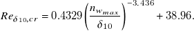 \begin{equation} Re_{\delta _{10},cr} = 0.4329 {\left ( \dfrac {n_{w_{max}}}{\delta _{10}} \right )^{-3.436}} + 38.96. \end{equation}
Equation (2) (Xu et al. (Reference Xu, Han, Qiao, Bai and Zhang2019)) approximates the data presented in Dagenhart (Reference Dagenhart1981, Figure 12).
To compute the growth rate $\sigma$
of a cross-flow instability with wavenumber
$\sigma$
of a cross-flow instability with wavenumber $\beta$
for a boundary layer profile characterised by
$\beta$
for a boundary layer profile characterised by $\delta _{10}$
,
$\delta _{10}$
, $n_{w_{max}}$
and
$n_{w_{max}}$
and $Re_{\delta _{10}}$
, the following procedure is applied by Dagenhart:
$Re_{\delta _{10}}$
, the following procedure is applied by Dagenhart:
-
(i) Identify the stability chart of index $i$
corresponding to the velocity profile whose
$\left ( Re_{\delta _{10},cr} \right )_i$
is closest to
$Re_{\delta _{10},cr}$
.
$i$
corresponding to the velocity profile whose
$\left ( Re_{\delta _{10},cr} \right )_i$
is closest to
$Re_{\delta _{10},cr}$
. -
(ii) Define the adjusted Reynolds number
\begin{equation*}\widehat {Re}_{\delta _{10}} = Re_{\delta _{10}} + \left ( Re_{\delta _{10},cr} \right )_i - Re_{\delta _{10},cr}.\end{equation*}
-
(iii) Read
$\hat {\sigma }^*(\widehat {Re}_{\delta _{10}}, \beta \delta _{10} )$
from the selected stability chart. -
(iv) Finally, calculate the growth rate
$\sigma$
using the relation
\begin{equation*}\sigma \delta _{10} = \hat {\sigma }^* \dfrac {\left (\dfrac {w_{max}}{U_e} \right )}{\left (\dfrac {w_{max}}{U_e} \right )_i}.\end{equation*}


2.1.2 Perraud et al. (Reference Perraud, Arnal, Casalis, Archambaud and Donelli2009)
Given the inflectional origin of cross-flow instability (see Figures 1 and 2), Casalis and Arnal (Reference Casalis and Arnal1996) derived a model for unsteady cross-flow instability based on the characteristics of the generalised inflection point of the velocity profile $u_{\psi }$
in a plane rotated by an angle
$u_{\psi }$
in a plane rotated by an angle $\psi$
relative to the streamline direction. In this model,
$\psi$
relative to the streamline direction. In this model, $n_{gip}$
is the wall distance at which
$n_{gip}$
is the wall distance at which $\frac {d}{dn} \left ( \rho \frac {d u_\psi }{dn} \right )=0$
,
$\frac {d}{dn} \left ( \rho \frac {d u_\psi }{dn} \right )=0$
, $U_{gip} = {u}_\psi (n=n_{gip}) / U_e$
and
$U_{gip} = {u}_\psi (n=n_{gip}) / U_e$
and $P_{gip} = \left [ n / U_e \frac {d u_{\psi }}{{d} n}\right ]_{n=n_{gip}}$
(see Figure 2 for
$P_{gip} = \left [ n / U_e \frac {d u_{\psi }}{{d} n}\right ]_{n=n_{gip}}$
(see Figure 2 for $\psi =90^{\circ }$
).
$\psi =90^{\circ }$
).
A similar approach was later extended by Perraud et al. (Reference Perraud, Arnal, Casalis, Archambaud and Donelli2009) for stationary cross-flow instabilities. The model is expressed as
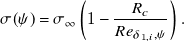 \begin{equation} \sigma (\psi ) = \sigma _\infty \left (1 - \dfrac {R_{c}}{Re_{\delta _{1,i},\psi }} \right ) .\end{equation}
In this model, $R_{c}$
depends on
$R_{c}$
depends on $P_{gip}$
while
$P_{gip}$
while $\sigma _{\infty }$
is a function of
$\sigma _{\infty }$
is a function of $U_{gip}$
. The Reynolds number
$U_{gip}$
. The Reynolds number $Re_{\delta _{1,i},\psi }$
is defined using the incompressible displacement thickness of the velocity profile
$Re_{\delta _{1,i},\psi }$
is defined using the incompressible displacement thickness of the velocity profile $u_{\psi }$
.
$u_{\psi }$
.
The corresponding $N$
-factors can then be computed as
$N$
-factors can then be computed as
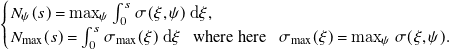 \begin{equation} \begin{cases} N_\psi (s) = \max _{\psi } \int _0^s \sigma (\xi , {\psi }) \, {\mathrm{d}} \xi ,\\ N_{\text{max}}(s) = \int _0^s \sigma _{\text{max}}{(\xi )} \, {\mathrm{d}} \xi \ \ \ \text{where here} \ \ \ \sigma _{\text{max}}(\xi )=\max _{\psi } \sigma (\xi , \psi ). \end{cases} \end{equation}
Here, $N_{\psi }$
is closely related to
$N_{\psi }$
is closely related to $N_\beta$
because ‘a fixed value of
$N_\beta$
because ‘a fixed value of $\beta$
is associated with a practically constant value of
$\beta$
is associated with a practically constant value of $\psi$
’ (Arnal et al. (Reference Arnal, Casalis and Houdeville2008)).
$\psi$
’ (Arnal et al. (Reference Arnal, Casalis and Houdeville2008)).
2.1.3 Xu et al. (Reference Xu, Han, Qiao, Bai and Zhang2019)
From stability computations on Falkner–Skan–Cooke boundary layer profiles, Xu et al. (Reference Xu, Han, Qiao, Bai and Zhang2019) derived the following model for the cross-flow instability growth rate:
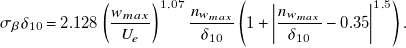 \begin{equation} \sigma _{\beta } \delta _{10} = 2.128 \left (\dfrac {w_{max}}{U_e}\right )^{1.07} \dfrac {n_{w_{max}}}{\delta _{10}} \left (1 + \left | \dfrac {n_{w_{max}}}{\delta _{10}}-0.35 \right |^{1.5}\right ) .\end{equation}
Here, $\sigma _\beta$
is defined such that
$\sigma _\beta$
is defined such that
 \begin{equation} N_\beta (s) = \int _0^s \sigma _\beta (\xi ) \, {\mathrm{d}} \xi .\end{equation}
2.1.4 Arnal et al. (Reference Arnal, Habiballah and Coustols1984) and Langtry et al. (Reference Langtry, Sengupta, Yeh and Dorgan2015)
Unlike the previous models, the models by Arnal et al. (Reference Arnal, Habiballah and Coustols1984) and Langtry et al. (Reference Langtry, Sengupta, Yeh and Dorgan2015) do not predict the growth rate of cross-flow instabilities but instead directly determine the transition location:
-
• Langtry et al. (Reference Langtry, Sengupta, Yeh and Dorgan2015) developed a RANS transition model that accounts for cross-flow transition. This model relies on the so-called non-dimensional cross-flow strength defined as
$H_{cf} = n He / U$
, where
$He$
is the helicity given by
$He = \| \vec {U} \cdot \vec {\Omega } \| / U$
. Here,
$\vec {U}$
is the local velocity (and
$U$
its magnitude) and
$\vec {\Omega }$
is the vorticity. -
• The C1 (Arnal et al. (Reference Arnal, Habiballah and Coustols1984)) criterion defines the transition location based on a threshold value of
$Re_{\delta _2}$
where
$\delta _2$
is transverse displacement thickness.


3. Building a database of stationary cross-flow characteristics
In this section, the workflow used to compute a database of boundary layer profiles on swept wings and their associated stability characteristics with respect to stationary crossflow (CF) waves is presented. The diagram in Figure 3 illustrates how the process operates.
This workflow is quite similar to the optimisation process described by Sudhi et al. (Reference Sudhi, Radespiel and Badrya2023) for transonic airfoil design. The inputs of the workflow are the airfoil geometry and aerodynamic parameters: Reynolds number ( $Re_{\infty }$
), Mach number (
$Re_{\infty }$
), Mach number ( $M_{\infty }$
), (negative) angle of attack
$M_{\infty }$
), (negative) angle of attack $\alpha$
and sweep angle
$\alpha$
and sweep angle $\varphi$
. As outputs, the workflow generates the boundary layer profiles on the upper surface and the corresponding stability diagrams.
$\varphi$
. As outputs, the workflow generates the boundary layer profiles on the upper surface and the corresponding stability diagrams.
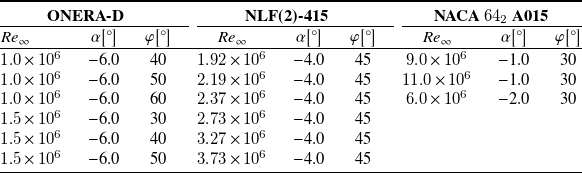
Table 1. Aerodynamic conditions for the ONERA-D airfoil
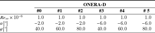
Table 2. Aerodynamic conditions for the NLF(2)-415 airfoil

Table 3. Aerodynamic conditions for the NACA $64_2$
A015 airfoil
$64_2$
A015 airfoil
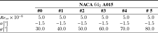

Figure 3. Database generation chain.
3.1 Chosen parameters
The ONERA-D, NLF(2)-415 and NACA $64_2$
A015 airfoils were selected to build the database. These three airfoils are known for their relevance in studying cross-flow transition (see respectively the references Schmitt and Manie (Reference Schmitt and Manie1979), Dagenhart and Saric (Reference Dagenhart and Saric1999) and Boltz et al. Reference Boltz, Kenyon and Allen(1960)). For each airfoil, six sets of aerodynamic conditions were chosen, as detailed in tables 1, 2 and 3. Different angles of attack (
$64_2$
A015 airfoils were selected to build the database. These three airfoils are known for their relevance in studying cross-flow transition (see respectively the references Schmitt and Manie (Reference Schmitt and Manie1979), Dagenhart and Saric (Reference Dagenhart and Saric1999) and Boltz et al. Reference Boltz, Kenyon and Allen(1960)). For each airfoil, six sets of aerodynamic conditions were chosen, as detailed in tables 1, 2 and 3. Different angles of attack ( $\alpha$
) and sweep (
$\alpha$
) and sweep ( $\phi$
) were selected to broaden the range of the cross-flow profiles. These angles were chosen such that stationary cross-flow instabilities develop on the upper surface of the airfoil. No more than six sets of aerodynamic conditions per airfoil were selected to limit the size of the database. The chord Reynolds number value is not crucial for deriving the model as the boundary layer profiles are rescaled when computing the stability diagram (see section 3.4). Therefore,
$\phi$
) were selected to broaden the range of the cross-flow profiles. These angles were chosen such that stationary cross-flow instabilities develop on the upper surface of the airfoil. No more than six sets of aerodynamic conditions per airfoil were selected to limit the size of the database. The chord Reynolds number value is not crucial for deriving the model as the boundary layer profiles are rescaled when computing the stability diagram (see section 3.4). Therefore, $Re_{{\infty }} = 5 \times 10^{6}$
was chosen for all cases. The Mach numbers are selected within the incompressible regime, specifically
$Re_{{\infty }} = 5 \times 10^{6}$
was chosen for all cases. The Mach numbers are selected within the incompressible regime, specifically ${M_\infty \in } [0.05, 0.22]$
. This choice is not critical, as stationary cross-flow instabilities exhibit nearly identical behaviour in both incompressible and transonic flows (Arnal (Reference Arnal1994)).
${M_\infty \in } [0.05, 0.22]$
. This choice is not critical, as stationary cross-flow instabilities exhibit nearly identical behaviour in both incompressible and transonic flows (Arnal (Reference Arnal1994)).
3.2 Inviscid pressure distribution computation
The pressure distribution is computed using the ISES software (Drela and Giles (Reference Drela and Giles1987)) and the simple sweep theory (Meier (Reference Meier2010)). Unlike the approach used by Sudhi et al. (Reference Sudhi, Radespiel and Badrya2023), ISES is run with the inviscid model, where only the two-dimensional (2-D) Euler equations are solved using the finite volume method without coupling to the integral boundary layer equations. The simple sweep theory is then applied to extend the 2-D computation to the 2.5-D flow, allowing the pressure distribution around an infinite swept wing to be calculated.
3.3 Solving of the boundary layer equations
Following the infinite swept-wing assumptions (i.e. invariance is assumed along the span), the velocity at the boundary layer edge is derived from the pressure distribution. The dimensionless results computed by ISES are dimensionalised using the following upstream temperature and pressure: $T_\infty = 300 K$
and
$T_\infty = 300 K$
and $P_\infty =101325 Pa$
. This velocity distribution is then used as input for the boundary layer equation solver 3C3D (Houdeville (Reference Houdeville1992)) (in contrast, Sudhi et al. (Reference Sudhi, Radespiel and Badrya2023) used the COCO solver). The 3C3D solver employs the method of characteristics and finite difference discretisation to solve the 3-D boundary layer equations. Although the solver can handle laminar, transitional and turbulent flows, only laminar flow computations are considered in this study. The equations are solved using a marching method, starting from the leading edge. However, the solver cannot account for upstream characteristics, meaning it halts when separation occurs.
$P_\infty =101325 Pa$
. This velocity distribution is then used as input for the boundary layer equation solver 3C3D (Houdeville (Reference Houdeville1992)) (in contrast, Sudhi et al. (Reference Sudhi, Radespiel and Badrya2023) used the COCO solver). The 3C3D solver employs the method of characteristics and finite difference discretisation to solve the 3-D boundary layer equations. Although the solver can handle laminar, transitional and turbulent flows, only laminar flow computations are considered in this study. The equations are solved using a marching method, starting from the leading edge. However, the solver cannot account for upstream characteristics, meaning it halts when separation occurs.
3.4 Local linear stability computations
Finally, the 1,260 boundary layer profiles computed by 3C3D are passed to ONERA’s in-house linear stability solver MAMOUT (Brazier (Reference Brazier2015)) (the linear stability LILO solver is used in the work of Sudhi et al. (Reference Sudhi, Radespiel and Badrya2023)). The local linear stability equations are discretised by means of a compact finite differences method.
For each case presented in tables 1, 2 and 3, the stability diagrams $\sigma ^*(Re_{\delta _{10}}, \beta ^*)$
(with
$\sigma ^*(Re_{\delta _{10}}, \beta ^*)$
(with $\sigma ^* = \sigma \times \delta _{10}$
and
$\sigma ^* = \sigma \times \delta _{10}$
and $\beta ^* = \beta \times \delta _{10}$
) are computed at every available station along the wing. For 23 boundary layer profiles, no unstable stationary CF mode is found and the automated stability chart computation fails and these profiles are discarded. Figures 4, 5 and 6 show the locations on each airfoil where the stability diagrams are computed.
$\beta ^* = \beta \times \delta _{10}$
) are computed at every available station along the wing. For 23 boundary layer profiles, no unstable stationary CF mode is found and the automated stability chart computation fails and these profiles are discarded. Figures 4, 5 and 6 show the locations on each airfoil where the stability diagrams are computed.

Figure 4. The NLF(2)-415 airfoil, the grey region indicates the locations where stability diagrams are computed.

Figure 5. The NACA $64_2$
A015 airfoil, the grey region indicates the locations where stability diagrams are computed.
$64_2$
A015 airfoil, the grey region indicates the locations where stability diagrams are computed.
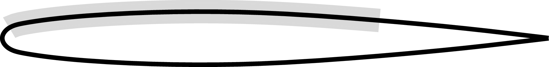
Figure 6. The ONERAD airfoil, the grey region indicates the locations where stability diagrams are computed.
The different values of $Re_{\delta _{10}}$
used to build the stability diagram are obtained by rescaling the boundary layer profiles. This is achieved by multiplying the two velocity components,
$Re_{\delta _{10}}$
used to build the stability diagram are obtained by rescaling the boundary layer profiles. This is achieved by multiplying the two velocity components, $u$
and
$u$
and $w$
, of the boundary layer profiles by
$w$
, of the boundary layer profiles by $Re_{\delta _{10}} / \widetilde {Re}_{\delta _{10}}$
, where
$Re_{\delta _{10}} / \widetilde {Re}_{\delta _{10}}$
, where $\widetilde {Re}_{\delta _{10}}$
is the value of
$\widetilde {Re}_{\delta _{10}}$
is the value of $Re_{\delta _{10}}$
without rescaling of the boundary layer profiles.
$Re_{\delta _{10}}$
without rescaling of the boundary layer profiles.
As an example, the stability diagram obtained for case no. 1 of the NLF(2)-0415 airfoil at $x/c \approx 1.6\%$
is plotted in Figure 7.
$x/c \approx 1.6\%$
is plotted in Figure 7.
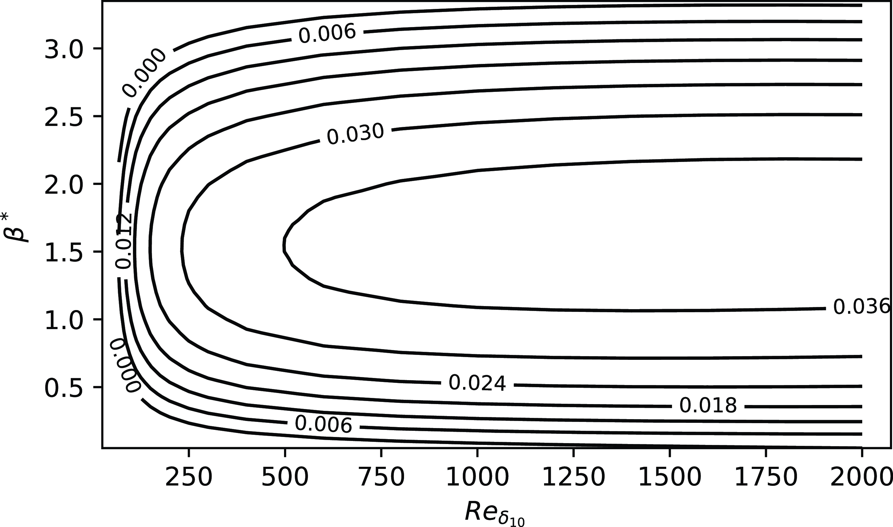
Figure 7.
Stability diagram $\sigma ^*(Re_{\delta _{10}}, \beta ^*)$
, case no. 1 of the NLF(2)-0415 airfoil at
$\sigma ^*(Re_{\delta _{10}}, \beta ^*)$
, case no. 1 of the NLF(2)-0415 airfoil at $x/c \approx 1.6\%$
.
$x/c \approx 1.6\%$
.
4. Derivation of model by means of symbolic regression
In this section, the pysr library (Cranmer (Reference Cranmer2023)) is used to derive models for $\sigma _{\text{max}}$
and
$\sigma _{\text{max}}$
and $\sigma$
from the database built in section 3. The aim is to provide accurate models for computing
$\sigma$
from the database built in section 3. The aim is to provide accurate models for computing $N_\beta$
and
$N_\beta$
and $N_{\text{max}}$
that are easier to implement and use than those developed by Dagenhart (Reference Dagenhart1981) and Perraud et al. (Reference Perraud, Arnal, Casalis, Archambaud and Donelli2009).
$N_{\text{max}}$
that are easier to implement and use than those developed by Dagenhart (Reference Dagenhart1981) and Perraud et al. (Reference Perraud, Arnal, Casalis, Archambaud and Donelli2009).
Only two open-source, easy-to-install Python libraries were found for symbolic regression: gplearn and pysr.Footnote
2
Initial tests showed that pysr significantly outperforms gplearn for the cases considered here, both in terms of accuracy and computational efficiency. pysr is based on a multi-population, multi-evolution evolutionary algorithm and is highly customisable. The standard binary operators addition, subtraction, multiplication and division – are selected, along with the unary operators: logarithm ( $\log$
), hyperbolic tangent (
$\log$
), hyperbolic tangent ( $\tanh$
) and inverse (
$\tanh$
) and inverse ( $x \rightarrow 1/x$
). Additional regressor settings prevent variables from appearing in exponents and limit the nesting of the operators
$x \rightarrow 1/x$
). Additional regressor settings prevent variables from appearing in exponents and limit the nesting of the operators $\tanh$
and
$\tanh$
and $\log$
. During symbolic learning, 70 % of the data are randomly selected for training, and the remaining 30 % are used for validation. Consequently, the validation set corresponds to interpolation. There is no a priori reason to expect the resulting symbolic expressions to yield accurate results in extrapolation.
$\log$
. During symbolic learning, 70 % of the data are randomly selected for training, and the remaining 30 % are used for validation. Consequently, the validation set corresponds to interpolation. There is no a priori reason to expect the resulting symbolic expressions to yield accurate results in extrapolation.
The regressor inputs are based on cross-flow boundary layer variables used in the models presented in section 2.1: $\delta _{10}$
,
$\delta _{10}$
, $n_{w_{max}}$
,
$n_{w_{max}}$
, $w_{max}$
,
$w_{max}$
, $Re_{\delta _{10}}$
(models of Dagenhart (Reference Dagenhart1981) and Xu et al. (Reference Xu, Han, Qiao, Bai and Zhang2019), see sections 2.1.1 and 2.1.3),
$Re_{\delta _{10}}$
(models of Dagenhart (Reference Dagenhart1981) and Xu et al. (Reference Xu, Han, Qiao, Bai and Zhang2019), see sections 2.1.1 and 2.1.3), $H_{cf,max}$
(maximum value of
$H_{cf,max}$
(maximum value of $H_{cf}$
in the boundary layer, defined by Langtry et al. (Reference Langtry, Sengupta, Yeh and Dorgan2015), see section 2.1.4),
$H_{cf}$
in the boundary layer, defined by Langtry et al. (Reference Langtry, Sengupta, Yeh and Dorgan2015), see section 2.1.4), $n_{gip}$
,
$n_{gip}$
, $U_{gip}$
,
$U_{gip}$
, $P_{gip}$
(model of Perraud et al. (Reference Perraud, Arnal, Casalis, Archambaud and Donelli2009), see section 2.1.2; only
$P_{gip}$
(model of Perraud et al. (Reference Perraud, Arnal, Casalis, Archambaud and Donelli2009), see section 2.1.2; only $\psi = 90 ^{\circ }$
is considered here) and
$\psi = 90 ^{\circ }$
is considered here) and $\delta _{2}$
(model of Arnal et al. (Reference Arnal, Habiballah and Coustols1984), see section 2.1.4). Additional boundary layer quantities are also included:
$\delta _{2}$
(model of Arnal et al. (Reference Arnal, Habiballah and Coustols1984), see section 2.1.4). Additional boundary layer quantities are also included: $\delta _1$
(displacement thickness),
$\delta _1$
(displacement thickness), $\theta _{11}$
(momentum thickness) and
$\theta _{11}$
(momentum thickness) and $U_e$
(velocity at the boundary layer edge). The composite variable
$U_e$
(velocity at the boundary layer edge). The composite variable $C_f Re_{\theta _{11}}$
is also used, where
$C_f Re_{\theta _{11}}$
is also used, where $C_f$
is the skin friction coefficient defined as
$C_f$
is the skin friction coefficient defined as $C_f = \tau _w / (1/2 \rho _e U_e^2)$
, with
$C_f = \tau _w / (1/2 \rho _e U_e^2)$
, with $\rho _e$
the density at the boundary layer edge,
$\rho _e$
the density at the boundary layer edge, $\tau _w$
the wall shear stress and
$\tau _w$
the wall shear stress and $Re_{\theta _{11}} = \theta _{11} U_e / \nu _e$
.
$Re_{\theta _{11}} = \theta _{11} U_e / \nu _e$
.
These quantities are combined to form 21 dimensionless variables: $H_{cf,max}$
,
$H_{cf,max}$
, $P_{gip}$
,
$P_{gip}$
, $C_f Re_{\theta _{11}}$
,
$C_f Re_{\theta _{11}}$
, $\delta _2 / \delta _1$
,
$\delta _2 / \delta _1$
, $\theta _{11} / \delta _1$
,
$\theta _{11} / \delta _1$
, $\theta _{11} / \delta _2$
,
$\theta _{11} / \delta _2$
, $n_{w_{max}} / \delta _1$
,
$n_{w_{max}} / \delta _1$
, $n_{w_{max}} / \delta _2$
,
$n_{w_{max}} / \delta _2$
, $n_{w_{max}} / \theta _{11}$
,
$n_{w_{max}} / \theta _{11}$
, $\delta _{10} / \delta _1$
,
$\delta _{10} / \delta _1$
, $\delta _{10} / \delta _2$
,
$\delta _{10} / \delta _2$
, $\delta _{10} / \theta _{11}$
,
$\delta _{10} / \theta _{11}$
, $\delta _{10} / n_{w_{max}}$
,
$\delta _{10} / n_{w_{max}}$
, $n_{gip} / \delta _1$
,
$n_{gip} / \delta _1$
, $n_{gip} / \delta _2$
,
$n_{gip} / \delta _2$
, $n_{gip} / \theta _{11}$
,
$n_{gip} / \theta _{11}$
, $n_{gip} / n_{w_{max}}$
,
$n_{gip} / n_{w_{max}}$
, $n_{gip} / \delta _{10}$
,
$n_{gip} / \delta _{10}$
, $w_{max} / U_e$
,
$w_{max} / U_e$
, $u_{gip} / U_e$
and
$u_{gip} / U_e$
and $u_{gip} / w_{max}$
. Redundancy is expected among these cross-flow variables, but the parsimony constraint imposed by the symbolic regression algorithm ensures that only the most relevant parameters are retained. Moreover, while variables such as
$u_{gip} / w_{max}$
. Redundancy is expected among these cross-flow variables, but the parsimony constraint imposed by the symbolic regression algorithm ensures that only the most relevant parameters are retained. Moreover, while variables such as $\theta _{11} / \delta _2$
could be computed by combining
$\theta _{11} / \delta _2$
could be computed by combining $\theta _{11} / \delta _1$
and
$\theta _{11} / \delta _1$
and $\delta _2 / \delta _1$
, doing so would incur a higher cost under the parsimony constraint in pysr than directly including
$\delta _2 / \delta _1$
, doing so would incur a higher cost under the parsimony constraint in pysr than directly including $\theta _{11} / \delta _2$
.
$\theta _{11} / \delta _2$
.
As the pysr algorithm involves randomness, each regression is run 20 times and the best-performing model is retained.
4.1 Expression for
$\sigma _{\text{max}}$

The variable $Re_{\delta _{10}}$
is added to the input dataset, and
$Re_{\delta _{10}}$
is added to the input dataset, and $\sigma _{\text{max}}^* = \sigma _{\text{max}} \times \delta _{10}$
is set as the output. The latter is obtained by extracting the maximum value of
$\sigma _{\text{max}}^* = \sigma _{\text{max}} \times \delta _{10}$
is set as the output. The latter is obtained by extracting the maximum value of $\sigma ^*$
from the stability diagram at each
$\sigma ^*$
from the stability diagram at each $Re_{\delta _{10}}$
(see Figure 7).
$Re_{\delta _{10}}$
(see Figure 7).
The resulting input database consists of 22 variables and 25,604 entries.
The following expression is returned by pysr:
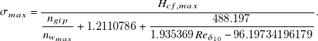 \begin{equation} \sigma _{max} = \dfrac {H_{cf,max}}{\dfrac {n_{gip}}{n_{w_{max}}} + 1.2110786 + \dfrac {488.197}{1.935369 Re_{\delta _{10}} - 96.19734196179}}. \end{equation}
As expected from Figure 7, pysr returns an increasing function with respect to $Re_{\delta _{10}}$
which asymptotically approaches a limit. This expression yields a critical Reynolds number
$Re_{\delta _{10}}$
which asymptotically approaches a limit. This expression yields a critical Reynolds number $Re_{\delta _{10},cr} = 49.7$
. This constant value aligns well with Figure 12 of Dagenhart (Reference Dagenhart1981) given the values of
$Re_{\delta _{10},cr} = 49.7$
. This constant value aligns well with Figure 12 of Dagenhart (Reference Dagenhart1981) given the values of ${\delta _{10} / n_{w_{max}}} \in [0.30, 0.53]$
found in the database computed in section 3. The parameter
${\delta _{10} / n_{w_{max}}} \in [0.30, 0.53]$
found in the database computed in section 3. The parameter $\sigma _{max}$
is found to depend solely on boundary layer quantities related to the cross-flow velocity profile.
$\sigma _{max}$
is found to depend solely on boundary layer quantities related to the cross-flow velocity profile.
The aim of this paper is to develop and validate a model for the growth rate of stationary cross-flow instabilities, rather than to conduct a sensitivity analysis. Therefore, all digits provided by pysr are retained.
Since the derived model consists of a relatively simple expression for the growth rate of stationary cross-flow instabilities, it could be combined with the amplification factor transport method of Coder and Maughmer (Reference Coder and Maughmer2014) for predicting transition in RANS CFD (Computational Fluid Dynamics) software. This integration could be implemented in a CFD solver capable of computing quantities along wall-normal lines (Cliquet et al. (Reference Cliquet, Houdeville and Arnal2008), Pascal (Reference Pascal2023)).
On the one hand, the proposed model for $N_{\text{max}}$
requires:
$N_{\text{max}}$
requires:
-
(i) Computing the boundary layer parameters
$H_{\text{cf,max}}$
,
$n_{\text{gip}}$
,
$n_{w_{\text{max}}}$
and
$Re_{\delta _{10}}$
at each location; and -
(ii) Evaluating Equation (7) at each location and computing the integral (1).


On the other hand, exact linear stability analysis requires:
-
(i) Solving an eigenvalue problem to compute
$\sigma (\xi , \beta )$
at each location for multiple
$\beta$
values (typically
$\geq 12$
); and -
(ii) Evaluating Equation (1).


Therefore, the proposed model would significantly reduce the computation time, as demonstrated in section 5.2.
4.2 Expression for
$\sigma$

Compared with $\sigma _{\text{max}}$
, modelling
$\sigma _{\text{max}}$
, modelling $\sigma$
is more complex. An initial attempt was made to build a database using each point from every stability diagram computed in section 3. However, the formulas generated by pysr were unsatisfactory in terms of accuracy. Consequently, it was necessary to provide the model with a priori knowledge. The stability diagram in Figure 7 is characteristic of inflectional instabilities. For such cases, Casalis and Arnal (Reference Casalis and Arnal1996) modelled the growth rate using two half-parabolas. In this study, however, the wavelength is chosen as the parameter for the parabolas rather than the Reynolds number, and the proposed model is
$\sigma$
is more complex. An initial attempt was made to build a database using each point from every stability diagram computed in section 3. However, the formulas generated by pysr were unsatisfactory in terms of accuracy. Consequently, it was necessary to provide the model with a priori knowledge. The stability diagram in Figure 7 is characteristic of inflectional instabilities. For such cases, Casalis and Arnal (Reference Casalis and Arnal1996) modelled the growth rate using two half-parabolas. In this study, however, the wavelength is chosen as the parameter for the parabolas rather than the Reynolds number, and the proposed model is
 \begin{equation} \sigma (Re_{\delta _{10}}, \beta ) = \sigma _{\max } \left ( 1 - \left [ \dfrac {\beta - \beta _M}{\beta _k - \beta _M} \right ] \right )^2, \ \beta _k = \beta _0 \text{ if } \beta \lt \beta _M \text{ else } \beta _1 .\end{equation}
While $\sigma _{max}$
is already known (see Eq. (7)), additional regressions are required to model
$\sigma _{max}$
is already known (see Eq. (7)), additional regressions are required to model $\beta _0$
,
$\beta _0$
, $\beta _1$
and
$\beta _1$
and $\beta _M$
. Following the approach of Casalis and Arnal (Reference Casalis and Arnal1996), these three wavenumbers were initially sought in the form
$\beta _M$
. Following the approach of Casalis and Arnal (Reference Casalis and Arnal1996), these three wavenumbers were initially sought in the form
 \begin{equation} \beta _X \times \delta _{10} = a_X + b_X / Re_{\delta _{10}}, \end{equation}
where the subscript $X$
denotes either
$X$
denotes either $0$
,
$0$
, $1$
or
$1$
or $M$
. However, it was found that better agreement with the exact LST is achieved by setting
$M$
. However, it was found that better agreement with the exact LST is achieved by setting $a_0 = b_M =0$
.
$a_0 = b_M =0$
.
For each of the 1,237 available stability diagrams, an initial set of curve fits is performed to determine $\beta _M$
,
$\beta _M$
, $\beta _0$
and
$\beta _0$
and $\beta _1$
at each
$\beta _1$
at each $Re_{\delta _{10}}$
. A second set of curve fits is then conducted to compute the parameters
$Re_{\delta _{10}}$
. A second set of curve fits is then conducted to compute the parameters $b_0$
,
$b_0$
, $a_1$
,
$a_1$
, $b_1$
and
$b_1$
and $a_M$
for each stability diagram. In 86 cases, the regression coefficient
$a_M$
for each stability diagram. In 86 cases, the regression coefficient $R^2$
was below 0.95, and these diagrams were discarded. Finally, the parameters
$R^2$
was below 0.95, and these diagrams were discarded. Finally, the parameters $b_0$
,
$b_0$
, $a_1$
,
$a_1$
, $b_1$
and
$b_1$
and $a_M$
were regressed using pysr on a database containing 1,151 entries. The following formulas were obtained:
$a_M$
were regressed using pysr on a database containing 1,151 entries. The following formulas were obtained:
 \begin{equation*} \begin{cases} a_M = 1.0431601 + \left (3.2593474 - 0.007606023 \frac {n_{w_{max}}}{\delta _2} \right ) \tanh \left ( \left [ \frac {n_{gip}}{\delta _2} \frac {u_{gip}}{U_e} \right ]^{4.5976334} \right ), \\ b_0 = \left (3.83610767033565 \frac {\delta _{10}}{\theta _{11}} + 270.70172 \tanh (a_M)^{735.47253} \right ) \dfrac {\log \left ( \frac {\delta _{10}}{n_{w_{max}}} \right )}{\tanh \left ( \frac {n_{gip}}{\delta _{10}} \right )}, \\ a_1 = \dfrac {0.0049740043 b_0}{\tanh \left ( C_f Re_{\theta _{11}} \right )} - 2.93882 \frac {n_{gip}}{n_{w_{max}}} + 8.263331 ,\\ b_1 = 8.446098 \left [ \left ( \frac {\delta _{10}}{n_{w_{max}}} \right )^{1.7631726} + \left ( \frac {n_{w_{max}}}{\delta _{10}} \frac {\delta _1}{\theta _{11}} \right )^{4.8353176} \right ] \\ \phantom {b_1 } - 79.171326 \left ( a_1 + C_f Re_{\theta _{11}} \right ) - 53.115273 + 656.5801 \frac {n_{w_{max}}}{\delta _{10}} .\end{cases} \end{equation*}
While the expressions for $b_0$
,
$b_0$
, $a_1$
,
$a_1$
, $b_1$
and
$b_1$
and $a_M$
primarily depend on boundary layer cross-flow quantities, the streamwise-related variables
$a_M$
primarily depend on boundary layer cross-flow quantities, the streamwise-related variables $\delta _1$
,
$\delta _1$
, $\theta _{11}$
and
$\theta _{11}$
and $C_f Re_{\theta _{11}}$
also appear in the formulas. The cross-flow shape factor
$C_f Re_{\theta _{11}}$
also appear in the formulas. The cross-flow shape factor $n_{w_{max}}/\delta _{10}$
, as defined by Dagenhart (Reference Dagenhart1981), appears four times. In contrast to Eq. (7), no dependency on
$n_{w_{max}}/\delta _{10}$
, as defined by Dagenhart (Reference Dagenhart1981), appears four times. In contrast to Eq. (7), no dependency on $H_{cf,max}$
is observed.
$H_{cf,max}$
is observed.
5 Validation
5.1 The 2.5-D infinite swept wing: database airfoils
In this section, equations (7) and (8), derived earlier, are validated for infinite swept-wing configurations. The validation cases are constructed using the same tool chain as in section 3 (illustrated in Figure 3). While the same three airfoils are employed, the aerodynamic parameters are selected from existing experimental results published in Schmitt and Manie (Reference Schmitt and Manie1979), Dagenhart and Saric (Reference Dagenhart and Saric1999) and Boltz et al. (Reference Boltz, Kenyon and Allen1960), and are listed in table 4 (with Mach numbers in the range $[0.05, 0.07]$
).
$[0.05, 0.07]$
).
Table 4. Aerodynamic parameters for validation computations
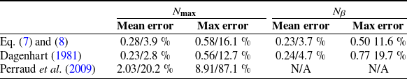
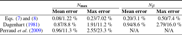
In tables 5, 6 and 7, the values of $N_{\text{max}}$
and
$N_{\text{max}}$
and $N_\beta$
computed by integrating the growth rate using equations (7) and (8) are compared with exact linear stability results from MAMOUT. These comparisons are made at locations where either
$N_\beta$
computed by integrating the growth rate using equations (7) and (8) are compared with exact linear stability results from MAMOUT. These comparisons are made at locations where either $N_{\text{max}}$
or
$N_{\text{max}}$
or $N_\beta$
exceeds 3.0. For each airfoil, the maximum and mean absolute and relative errors are reported. Additional comparisons are made with the methods of Dagenhart (Reference Dagenhart1981) and Perraud et al. (Reference Perraud, Arnal, Casalis, Archambaud and Donelli2009).Footnote
3
For
$N_\beta$
exceeds 3.0. For each airfoil, the maximum and mean absolute and relative errors are reported. Additional comparisons are made with the methods of Dagenhart (Reference Dagenhart1981) and Perraud et al. (Reference Perraud, Arnal, Casalis, Archambaud and Donelli2009).Footnote
3
For $N_\beta$
, comparisons were also made with the model of Xu et al. (Reference Xu, Han, Qiao, Bai and Zhang2019); however, this model consistently produced values at least twice those given by exact LST, rendering its inclusion in tables 5, 6 and 7 irrelevant.
$N_\beta$
, comparisons were also made with the model of Xu et al. (Reference Xu, Han, Qiao, Bai and Zhang2019); however, this model consistently produced values at least twice those given by exact LST, rendering its inclusion in tables 5, 6 and 7 irrelevant.
Table 5. Mean and maximum errors of $N$
-factors, ONERA-D airfoil
$N$
-factors, ONERA-D airfoil
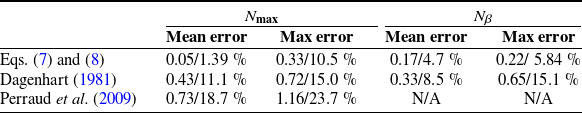
Table 6. Mean and maximum errors of $N$
-factors, NLF(2)-415 airfoil
$N$
-factors, NLF(2)-415 airfoil
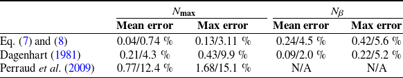
Table 7. Mean and maximum errors of $N$
-factors, NACA
$N$
-factors, NACA $64_2$
A015 airfoil
$64_2$
A015 airfoil
The proposed models, based on equations (7) and (8), yield satisfactory results for all three airfoils, for both $N_{\text{max}}$
and
$N_{\text{max}}$
and $N_\beta$
. The model by Dagenhart (Reference Dagenhart1981) delivers comparable accuracy. The method of Perraud et al. (Reference Perraud, Arnal, Casalis, Archambaud and Donelli2009) achieves only moderate accuracy for
$N_\beta$
. The model by Dagenhart (Reference Dagenhart1981) delivers comparable accuracy. The method of Perraud et al. (Reference Perraud, Arnal, Casalis, Archambaud and Donelli2009) achieves only moderate accuracy for $N_{\text{max}}$
. Among all models, the best and worst agreements are observed for the NLF(2)-415 airfoil and NACA
$N_{\text{max}}$
. Among all models, the best and worst agreements are observed for the NLF(2)-415 airfoil and NACA $64_2$
A015 airfoil, respectively. The excellent performance of the Dagenhart (Reference Dagenhart1981) model on the NLF(2)-415 airfoil was previously demonstrated in (Dagenhart and Saric (Reference Dagenhart and Saric1999)).
$64_2$
A015 airfoil, respectively. The excellent performance of the Dagenhart (Reference Dagenhart1981) model on the NLF(2)-415 airfoil was previously demonstrated in (Dagenhart and Saric (Reference Dagenhart and Saric1999)).
5.2 The 2.5-D infinite swept wing: NACA0012, DTP-A and DTP-B airfoils
While the derived models yield satisfactory results in section 5.1, their generalisability and robustness for infinite swept-wing computations are further assessed by considering airfoils that do not belong to the training database. Three cases relevant to the study of cross-flow instabilities (Arnal et al. (Reference Arnal, Piot, Archambaud, Casalis, Content, Dandois and Colamartino2007), Tokugawa et al. (Reference Tokugawa, Takagi, Ueda and Ido2005)) are considered in this section:
-
(i) NACA 0012 airfoil:
$\alpha =-12^{\circ }$
,
$\varphi =40 ^{\circ }$
and
$Q_\infty =20 m/s$
(upstream velocity). The upstream temperature and pressure are set to
$T_\infty = 300 K$
and
$P_\infty =101325 Pa$
, respectively. -
(ii) DTP-A airfoil:
$\alpha =0^{\circ }$
,
$\varphi =40 ^{\circ }$
,
$Q_\infty =36 m/s$
,
$Re_\infty =2.8 \times 10^6$
and
$P_\infty =101325 Pa$
. -
(iii) DTP-B airfoil:
$\alpha =6 ^{\circ }$
(the lower surface is considered),
$\varphi =40^{\circ }$
,
$Q_\infty =70 m/s$
,
$Re_\infty =3.26 {\times 10^6}$
and
$P_\infty =101325 Pa$
.


The validation process follows the same methodology as in section 5.1: the maximum and mean absolute and relative errors on $N_{\text{max}}$
and
$N_{\text{max}}$
and $N_\beta$
are presented in table 8. Errors are computed by comparing the results of exact linear stability computations performed with MAMOUT against those obtained using equations (7) and (8), as well as the models of Dagenhart (Reference Dagenhart1981) and Perraud et al. (Reference Perraud, Arnal, Casalis, Archambaud and Donelli2009). Only regions supporting cross-flow instabilities are retained by considering locations where either
$N_\beta$
are presented in table 8. Errors are computed by comparing the results of exact linear stability computations performed with MAMOUT against those obtained using equations (7) and (8), as well as the models of Dagenhart (Reference Dagenhart1981) and Perraud et al. (Reference Perraud, Arnal, Casalis, Archambaud and Donelli2009). Only regions supporting cross-flow instabilities are retained by considering locations where either $N_{max}$
or
$N_{max}$
or $N_\beta$
exceed 3.0.
$N_\beta$
exceed 3.0.
Table 8. Mean and maximum errors on $N$
-factors, NACA 0012, DTP-A and DTP-B airfoils
$N$
-factors, NACA 0012, DTP-A and DTP-B airfoils
The models defined by equations. (7) and (8) yield satisfactory results. The magnitudes of the mean and maximum errors are comparable to those obtained in section 5.1 (see in particular table 5). The derived models outperform those of Dagenhart (Reference Dagenhart1981) and Perraud et al. (Reference Perraud, Arnal, Casalis, Archambaud and Donelli2009) across all three cases. In particular, the model of Perraud et al. (Reference Perraud, Arnal, Casalis, Archambaud and Donelli2009) is once again found to provide only moderate accuracy.
All computations were performed on a single core of a workstation for the three cases considered in this section. Exact linear stability analysis with the MAMOUT solver required 58 minutes to compute $\sigma$
at each location and for 20 values of
$\sigma$
at each location and for 20 values of $\beta$
. Less than a second was then needed to evaluate both integrals
$\beta$
. Less than a second was then needed to evaluate both integrals $N_{\text{max}}$
and
$N_{\text{max}}$
and $N_\beta$
using Eq. (1). The simplified model derived in this paper reduced the computation time to 26 s for
$N_\beta$
using Eq. (1). The simplified model derived in this paper reduced the computation time to 26 s for $N_\beta$
and 16 s for
$N_\beta$
and 16 s for $N_{\text{max}}$
.
$N_{\text{max}}$
.
5.3 The 3-D prolate spheroid
Transition on the 3-D prolate spheroid with aspect ratio $a/b=1.2$
was measured by Kreplin et al. (Reference Kreplin, Vollmers and Meier1985). Flow conditions
$a/b=1.2$
was measured by Kreplin et al. (Reference Kreplin, Vollmers and Meier1985). Flow conditions $Re = 6.54 \times 10^6, \alpha =15^{\circ }$
were selected to ensure a transition scenario dominated by cross-flow instability (Stock (Reference Stock2006)). Despite the geometric and flow complexity in this configuration, the potential solution can be computed analytically following the approach of Cebeci et al. (Reference Cebeci, Hirsh and Kaups1978). The analytically derived velocity distribution is provided as input to 3C3D to compute the boundary layer velocity profiles over the geometry. The surface mesh is generated using step sizes of
$Re = 6.54 \times 10^6, \alpha =15^{\circ }$
were selected to ensure a transition scenario dominated by cross-flow instability (Stock (Reference Stock2006)). Despite the geometric and flow complexity in this configuration, the potential solution can be computed analytically following the approach of Cebeci et al. (Reference Cebeci, Hirsh and Kaups1978). The analytically derived velocity distribution is provided as input to 3C3D to compute the boundary layer velocity profiles over the geometry. The surface mesh is generated using step sizes of $1 ^{\circ }$
and
$1 ^{\circ }$
and $0.5 ^{\circ }$
along the angular coordinate
$0.5 ^{\circ }$
along the angular coordinate $\chi$
(with
$\chi$
(with $x=- a \cos (\chi )$
) and the polar angle
$x=- a \cos (\chi )$
) and the polar angle $\phi$
in the
$\phi$
in the $(y,z)$
plane, respectively. To avoid the velocity singularity at the leading edge, the mesh starts at
$(y,z)$
plane, respectively. To avoid the velocity singularity at the leading edge, the mesh starts at $\chi =\chi _{min}=0.049$
, corresponding to
$\chi =\chi _{min}=0.049$
, corresponding to $x/a=-0.9988$
.
$x/a=-0.9988$
.
The growth rate from linear stability analysis is computed at each location using ONERA’s in-house stability solver MAMOUT, as well as the models developed in this paper and that of Dagenhart (Reference Dagenhart1981). Growth-rate values are interpolated along 360 streamlines (relative to the potential flow), enabling the computation of $N$
-factors along each. The streamline starting locations are uniformly distributed along the azimuth (i.e. with a step size
$N$
-factors along each. The streamline starting locations are uniformly distributed along the azimuth (i.e. with a step size $\Delta \phi = 0.5 ^{\circ }$
) at
$\Delta \phi = 0.5 ^{\circ }$
) at $\chi = \chi _{min}$
.
$\chi = \chi _{min}$
.
The threshold value $N_{\beta }^T =5.5$
given by Stock (Reference Stock2006) is applied. According to Stock (Reference Stock2006, Figure 15 b), stationary cross-flow instability is dominant within the region
$N_{\beta }^T =5.5$
given by Stock (Reference Stock2006) is applied. According to Stock (Reference Stock2006, Figure 15 b), stationary cross-flow instability is dominant within the region $\phi \in [-135^{\circ }, -80^{\circ }]$
. This region is therefore the focus of the following discussion.
$\phi \in [-135^{\circ }, -80^{\circ }]$
. This region is therefore the focus of the following discussion.
5.3.1 Computation of
$N_{\text{max}}$

In this section, equation (7) is tested by comparing transition locations obtained using $N_{\text{max}}^T=8.2$
. This value is selected based on the ratio
$N_{\text{max}}^T=8.2$
. This value is selected based on the ratio $N_{\text{max}}^T / N_\beta ^T$
reported by Srokowski and Orszag (Reference Srokowski and Orszag1977) (see Appendix A.1). The resulting transition lines are shown in Figure 8 and compared with predictions from the model of Dagenhart (Reference Dagenhart1981) and with exact linear stability results from MAMOUT. Both the model developed in this study and that of Dagenhart (Reference Dagenhart1981) show strong agreement with exact stability results. However, equation (7) predicts a transition line that lies slightly upstream of the exact linear stability prediction, whereas the model of Dagenhart (Reference Dagenhart1981) places the transition line slightly downstream.
$N_{\text{max}}^T / N_\beta ^T$
reported by Srokowski and Orszag (Reference Srokowski and Orszag1977) (see Appendix A.1). The resulting transition lines are shown in Figure 8 and compared with predictions from the model of Dagenhart (Reference Dagenhart1981) and with exact linear stability results from MAMOUT. Both the model developed in this study and that of Dagenhart (Reference Dagenhart1981) show strong agreement with exact stability results. However, equation (7) predicts a transition line that lies slightly upstream of the exact linear stability prediction, whereas the model of Dagenhart (Reference Dagenhart1981) places the transition line slightly downstream.
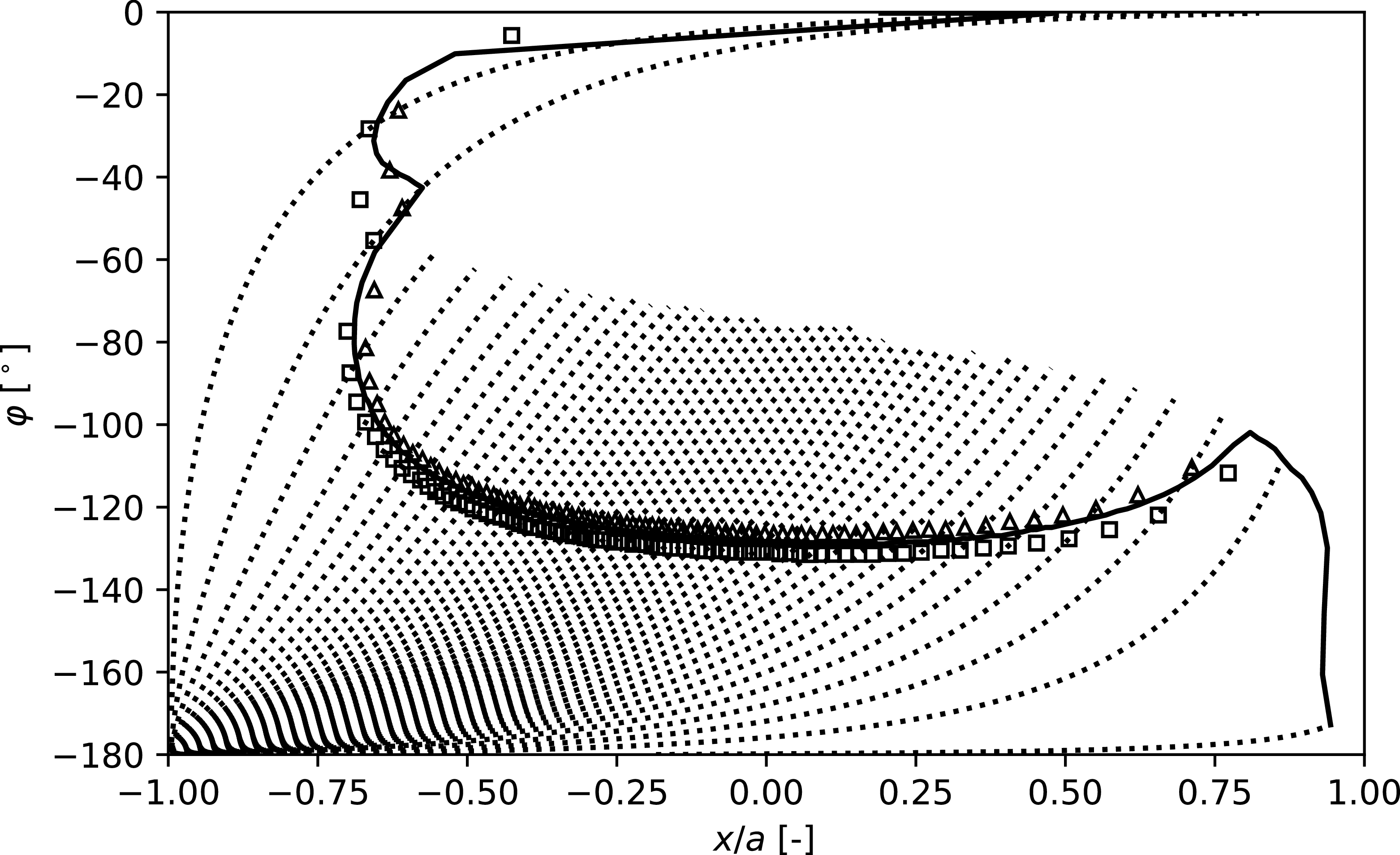
Figure 8.
Computed transition locations with eq. (7) ( $\Box {}$
), with the model of Dagenhart (Reference Dagenhart1981) (
$\Box {}$
), with the model of Dagenhart (Reference Dagenhart1981) ( $\triangle$
) and with MAMOUT (solid line). Streamlines are plotted as dotted lines.
$\triangle$
) and with MAMOUT (solid line). Streamlines are plotted as dotted lines.
5.3.2 Computation of
$N_\beta$

In this section, transition lines based on $N_\beta$
are computed and compared. Figure 9 shows that the transition lines obtained using equation (8) and the method of Dagenhart (Reference Dagenhart1981) align closely with the results of exact linear stability computation. As previously observed, the transition line predicted by equation (8) lies slightly upstream of the MAMOUT prediction, while the transition locations given by the method of Dagenhart (Reference Dagenhart1981) are found both upstream and downstream. Very good agreement is observed in the region of interest with the computations of Krimmelbein (Reference Krimmelbein2021), whereas the transition line computed by Stock (Reference Stock2006) appears slightly further downstream. No explanation can be offered for these discrepancies.
$N_\beta$
are computed and compared. Figure 9 shows that the transition lines obtained using equation (8) and the method of Dagenhart (Reference Dagenhart1981) align closely with the results of exact linear stability computation. As previously observed, the transition line predicted by equation (8) lies slightly upstream of the MAMOUT prediction, while the transition locations given by the method of Dagenhart (Reference Dagenhart1981) are found both upstream and downstream. Very good agreement is observed in the region of interest with the computations of Krimmelbein (Reference Krimmelbein2021), whereas the transition line computed by Stock (Reference Stock2006) appears slightly further downstream. No explanation can be offered for these discrepancies.
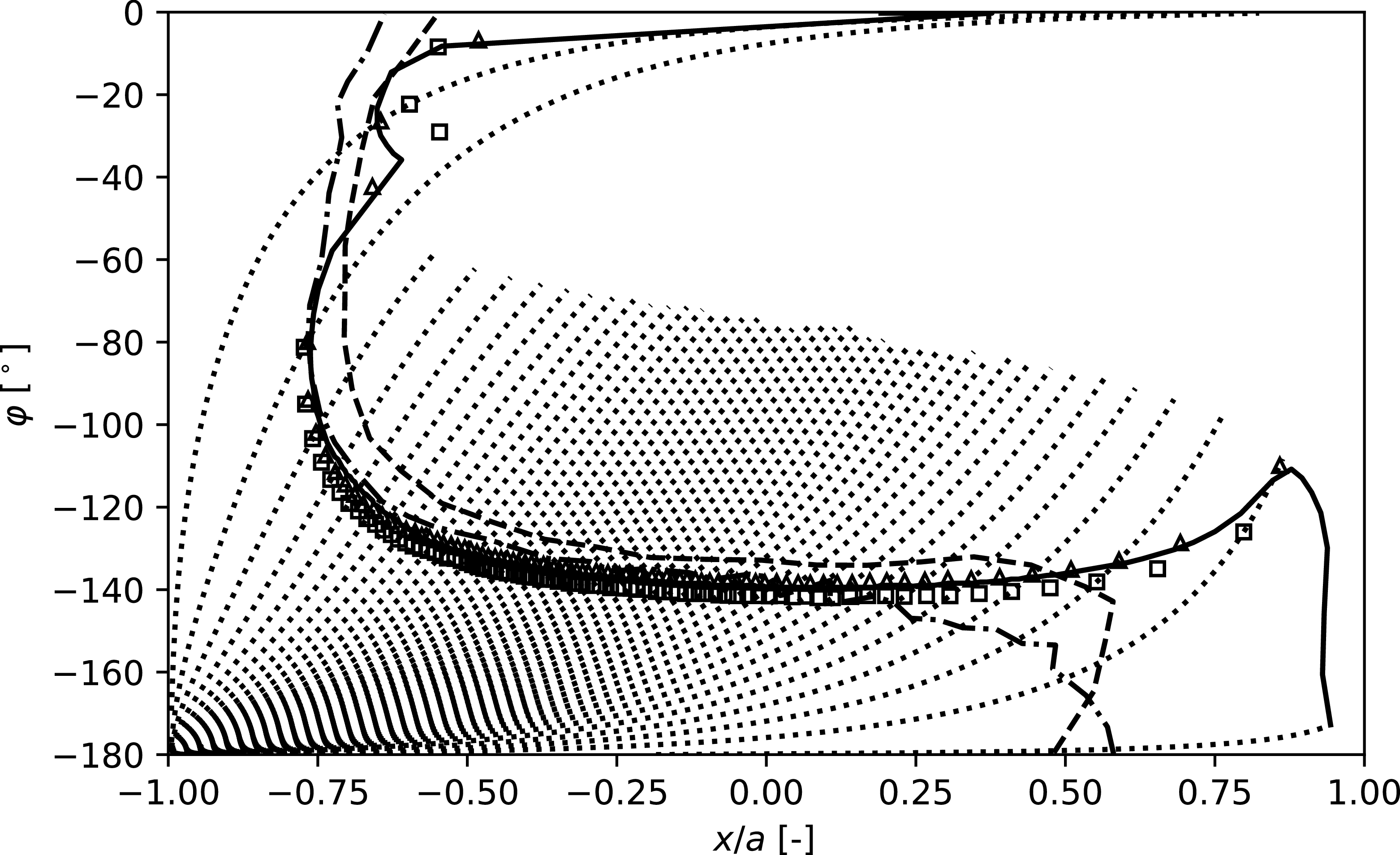
Figure 9.
Computed transition locations with eq. (8) ( $\Box$
), with the model of Dagenhart (Reference Dagenhart1981) (
$\Box$
), with the model of Dagenhart (Reference Dagenhart1981) ( $\triangle$
) and with MAMOUT (solid line). Streamlines are plotted as dotted lines. The transition lines computed by Krimmelbein (Reference Krimmelbein2021) and Stock (Reference Stock2006) are plotted as dash-dotted and dashed lines, respectively.
$\triangle$
) and with MAMOUT (solid line). Streamlines are plotted as dotted lines. The transition lines computed by Krimmelbein (Reference Krimmelbein2021) and Stock (Reference Stock2006) are plotted as dash-dotted and dashed lines, respectively.
6. Conclusions
In this study, a new model was derived to estimate the growth rate of stationary cross-flow instabilities, combining ease of use with good accuracy. The model was developed using a comprehensive database of 1,237 boundary layer profiles computed for three representative airfoils (ONERA-D, NLF(2)-415 and NACA $64_2$
A015) under a range of aerodynamic conditions. Linear stability characteristics of these profiles were analysed using the ONERA MAMOUT solver, and symbolic regression techniques were applied to derive expressions for the growth rate of cross-flow instabilities. As expected the resulting formulas were found to depend primarily on cross-flow boundary layer quantities.
$64_2$
A015) under a range of aerodynamic conditions. Linear stability characteristics of these profiles were analysed using the ONERA MAMOUT solver, and symbolic regression techniques were applied to derive expressions for the growth rate of cross-flow instabilities. As expected the resulting formulas were found to depend primarily on cross-flow boundary layer quantities.
Validation of the model on infinite swept-wing configurations showed satisfactory results. It performed consistently well across the ONERA-D and NLF(2)-415 airfoils. although slightly higher errors were observed for the NACA $64_2$
A015 airfoil. The new model outperforms the method of Perraud et al. (Reference Perraud, Arnal, Casalis, Archambaud and Donelli2009). The method of Dagenhart (Reference Dagenhart1981) yields slightly better accuracy on the NACA
$64_2$
A015 airfoil. The new model outperforms the method of Perraud et al. (Reference Perraud, Arnal, Casalis, Archambaud and Donelli2009). The method of Dagenhart (Reference Dagenhart1981) yields slightly better accuracy on the NACA $64_2$
A015 airfoil for
$64_2$
A015 airfoil for $N_\beta$
and on the NLF(2)-415 airfoil for
$N_\beta$
and on the NLF(2)-415 airfoil for $N_{\text{max}}$
. The new model also produces satisfactory results for configurations involving airfoils that are not part of the training database (NACA 0012, DTP-A, DTP-B).
$N_{\text{max}}$
. The new model also produces satisfactory results for configurations involving airfoils that are not part of the training database (NACA 0012, DTP-A, DTP-B).
To assess the predictive capability of the derived models on 3-D geometries, the prolate spheroid configuration was considered. Under flow conditions dominated by cross-flow instabilities, comparisons of transition lines based on $N_{\text{max}}$
and
$N_{\text{max}}$
and $N_\beta$
show that the models developed in this paper closely align with the results from exact linear stability computations. Specifically, the transition lines predicted using the growth-rate equations generally show excellent agreement with the MAMOUT results, with the model-based transition lines lying slightly upstream.
$N_\beta$
show that the models developed in this paper closely align with the results from exact linear stability computations. Specifically, the transition lines predicted using the growth-rate equations generally show excellent agreement with the MAMOUT results, with the model-based transition lines lying slightly upstream.
The proposed model offers a simpler and more accurate alternative to the model developed by Perraud et al. (Reference Perraud, Arnal, Casalis, Archambaud and Donelli2009), delivering improved precision without added complexity. Compared with the method by Dagenhart (Reference Dagenhart1981), the accuracy is comparable. However, the implementation of the present model is significantly more straightforward, as it eliminates the need for storage and interpolation of precomputed tables, making it highly practical for broader application in transition prediction.
The overall performance indicates that this model offers a robust and efficient tool for predicting cross-flow transition in boundary layers. Future work could focus on implementing the model in RANS solvers, with potential applications in aerodynamic design and optimisation.
Acknowledgements
The author acknowledges K. Dotse and V. Mouysset for providing the program used to compute streamlines on the prolate spheroid.
During the preparation of this work the author used ChatGPT and DeepSeek in order to improve language and readability. Moreover ChatGPT was used to generate a skeleton for the abstract. After using this AI tool, the author reviewed and edited the content as needed and takes full responsibility for the content of the publication.
Data availability statement
The data and code used in this work are currently proprietary and confidential.
Funding statement
The author gratefully acknowledges funding by the ONERA project MATRIX directed by F. Méry.
Competing interests
The author declares no conflict of interest.
Ethical standards
The research meets all ethical guidelines, including adherence to the legal requirements of the study country.
Appendix
A.1 Relationship between
$N_\beta$
and
$N_{\text{max}}$


Srokowski and Orszag (Reference Srokowski and Orszag1977) determined both $N_\beta ^T$
and
$N_\beta ^T$
and $N_{\text{max}}^T$
corresponding to the transition locations published by Boltz et al. (Reference Boltz, Kenyon and Allen1960) (for the NACA
$N_{\text{max}}^T$
corresponding to the transition locations published by Boltz et al. (Reference Boltz, Kenyon and Allen1960) (for the NACA $64_2$
A015 airfoil). They found that
$64_2$
A015 airfoil). They found that $N_\beta ^T \in [6.7,7.2]$
, corresponding to a spread of 7.2 % around the arithmetic mean while
$N_\beta ^T \in [6.7,7.2]$
, corresponding to a spread of 7.2 % around the arithmetic mean while $N^T_{\text{max}} \in [9.7,11]$
which corresponds to a spread of 6.1%.
$N^T_{\text{max}} \in [9.7,11]$
which corresponds to a spread of 6.1%.
A similar investigation using experimental results from Dagenhart and Saric (Reference Dagenhart and Saric1999) yielded $N_\beta ^T \in [5.6, 6.8]$
and
$N_\beta ^T \in [5.6, 6.8]$
and $N^T_{\text{max}} \in [6.9, 8.3]$
, resulting in relative spreads of
$N^T_{\text{max}} \in [6.9, 8.3]$
, resulting in relative spreads of $20.0\%$
and
$20.0\%$
and $18.5\%$
, respectively.
$18.5\%$
, respectively.
While both integration strategies are considered valid for transition prediction, $N_{\beta }^T$
is typically reported. Here, we attempt to deduce
$N_{\beta }^T$
is typically reported. Here, we attempt to deduce $N_{\text{max}}^T$
from
$N_{\text{max}}^T$
from $N_{\beta }^T$
. For each airfoil and set of flow conditions computed in section 5.1, a subset was created with
$N_{\beta }^T$
. For each airfoil and set of flow conditions computed in section 5.1, a subset was created with $N_\beta \gt 3$
, resulting in a dataset of 850 entries with 23 features (the 22 features from section 4.1 plus
$N_\beta \gt 3$
, resulting in a dataset of 850 entries with 23 features (the 22 features from section 4.1 plus $N_\beta$
). Using pysr as in section 4, we derived the following expression for
$N_\beta$
). Using pysr as in section 4, we derived the following expression for $N_{\text{max}} / N_\beta$
:
$N_{\text{max}} / N_\beta$
:
 \begin{equation} r = \dfrac {N_{\text{max}}}{N_\beta } = (p_{gip} + 1.1400409) \left ( \dfrac {\delta _2}{\theta _{11}} \left ( \dfrac {n_{gip}}{\delta _{10}} - 0.23753823 \right ) - 0.09712514 \right ) + 1.1903278 .\end{equation}
Equation (10) is validated on the 3-D prolate spheroid case from section 5.3. In Figure 10, transition lines computed using MAMOUT growth rates are plotted by comparing $N_{\beta }$
with
$N_{\beta }$
with $N_{\beta }^T$
and
$N_{\beta }^T$
and $N_{\text{max}}$
with
$N_{\text{max}}$
with $r \times N_{\beta }^T$
(only where
$r \times N_{\beta }^T$
(only where $N_{\text{max}}\gt N_{\beta }^T$
). The two transition lines display excellent agreement, demonstrating that using
$N_{\text{max}}\gt N_{\beta }^T$
). The two transition lines display excellent agreement, demonstrating that using $N_\beta ^T$
along with
$N_\beta ^T$
along with $r$
allows accurate prediction of the transition location based on
$r$
allows accurate prediction of the transition location based on $N_{\text{max}}$
computation.
$N_{\text{max}}$
computation.
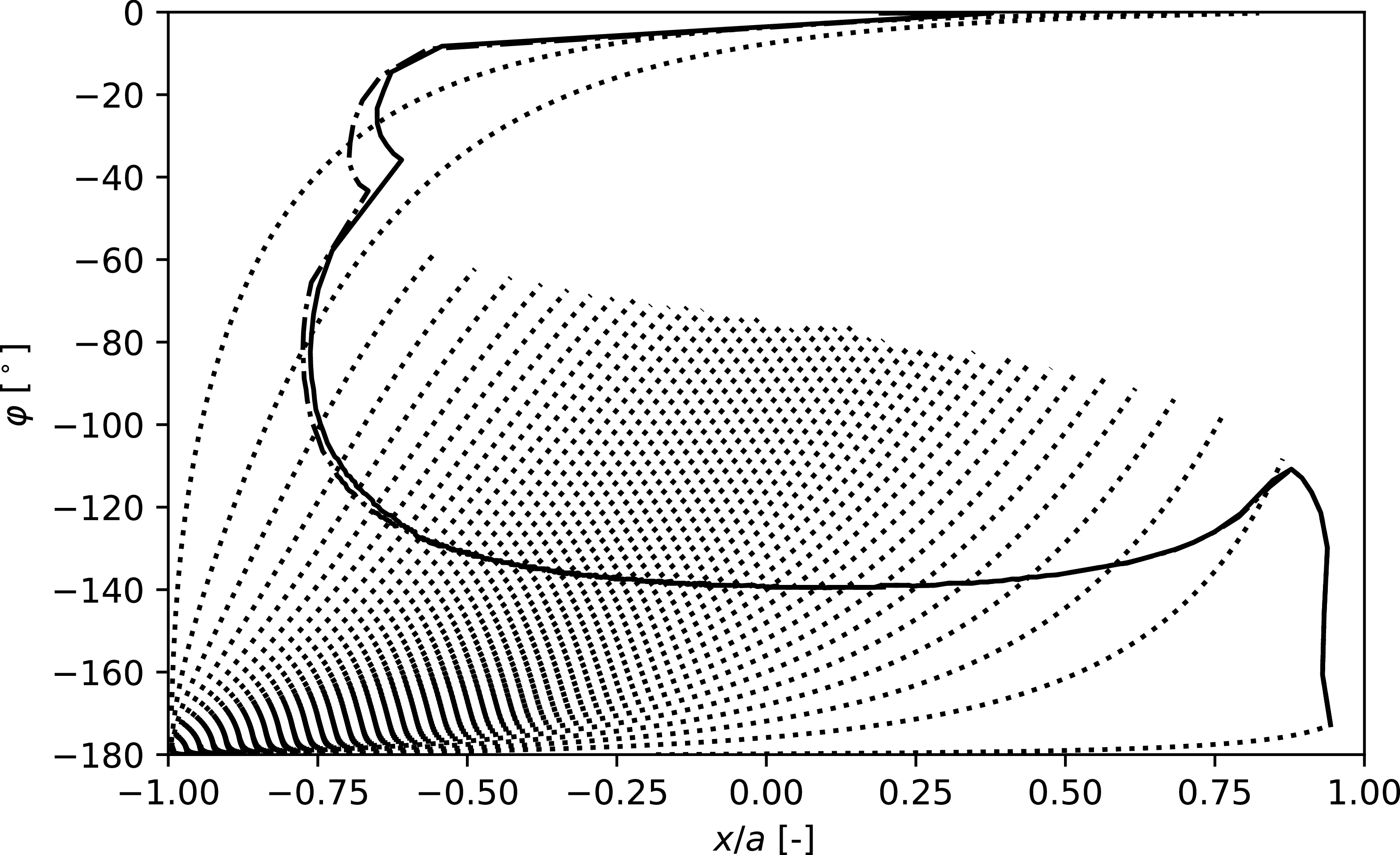
Figure 10.
Computed transition lines defined by $N_\beta =N_\beta ^T$
(solid line) and by
$N_\beta =N_\beta ^T$
(solid line) and by $N_{\text{max}} = r \times N_\beta ^T$
(dash-dotted line). Streamlines are plotted as dotted lines.
$N_{\text{max}} = r \times N_\beta ^T$
(dash-dotted line). Streamlines are plotted as dotted lines.


 Open access