


Impact Statement
With the maritime industry’s focus on reduced emissions and sustainability, drag reduction in ships is receiving growing attention. Air lubrication, a frictional drag reduction method, involves injecting air beneath the ship’s hull to minimise its contact with the surrounding, often turbulent flow. The morphology and dynamics of the air cavity formed, aspects crucial to air lubrication, are intrinsically linked to the incoming flow conditions. We experimentally investigate one aspect of this two-way coupling: the response of a turbulent boundary layer (TBL) to an air cavity formed under a specific incoming flow condition. Using single- and two-point statistics, we characterise the TBL development over the air cavity and examine the influence of different cavity regions on the TBL. Results and conclusions from this study are expected to not only provide insights regarding air cavity formation, but also establish a baseline reference for future studies examining variable inflow conditions and external perturbations.
1. Introduction
Turbulent flows are ubiquitous in nature and many engineering applications, and are often subject to external perturbations that can emanate from the free stream or the geometry over which they develop in the case of wall-bounded flows. For instance, in nature, the topographical features of the Earth in the form of “surface roughness” can perturb the often turbulent, atmospheric boundary layer. Flows encountered in engineering applications such as those over curved geometries (for example airfoils) or in turbomachinery, can be subject to a range of pressure gradients and curvatures that can have significant influence on the flow and, hence, the performance of the system.
Within this context, the creation of an air cavity in the path of an incoming turbulent boundary layer (TBL) is an example typically encountered in air lubrication or air layer drag reduction (ALDR) employed in ships (Elbing et al. Reference Elbing, Winkel, Lay, Ceccio, Dowling and Perlin2008; Mäkiharju, Perlin & Ceccio Reference Mäkiharju, Perlin and Ceccio2012). Briefly, the method of ALDR involves the injection of air (above a critical flow rate) below the ship’s hull which develops into a layer or a cavity, separating the surrounding liquid and the solid surface and thereby significantly reducing the skin-friction drag. The air cavity thickness, its length and stability, important parameters in the technique of ALDR, have been reported to be dependent on the incoming flow conditions (Nikolaidou et al. Reference Nikolaidou, Laskari, van Terwisga and Poelma2024; Zverkhovskyi Reference Zverkhovskyi2014). In addition to the incoming flow conditions and the air flow rate employed, the morphology and stability of the air cavity formed is dependent on the way the air is introduced below the ship’s hull. Common methods include employing a cavitator (similar to a backward-facing step) (Zverkhovskyi Reference Zverkhovskyi2014) or a slot-type injector (Elbing et al. Reference Elbing, Winkel, Lay, Ceccio, Dowling and Perlin2008; Nikolaidou et al. Reference Nikolaidou, Laskari, van Terwisga and Poelma2024). In this study, we report experimental findings on a typical case within the method of slot injection: the behaviour of an incoming TBL encountering a slot-injected air cavity formed at a specific incoming flow condition and air flow rate.
The flow over the air cavity encountered here is in some ways geometrically similar to solid bump flows studied in the literature (for example Baskaran et al. (Reference Baskaran, Smits and Joubert1987); Webster et al. (Reference Webster, DeGraff and Eaton1996)). The incoming TBL is perturbed by the obstruction created by an air cavity in its path, and this creates a local change in boundary condition. The change in the local boundary condition from a no slip at the wall to a free-slip boundary, the presence of a relatively variable obstacle geometry inherent to the dynamic nature of the air cavity, and the presence of multiple pressure gradients and curvatures, significantly increases the complexity of the current study relative to solid bump flows.
In an experimental study of a TBL moving over a two-dimensional curved hill by Baskaran et al. (Reference Baskaran, Smits and Joubert1987), the TBL was subjected to multiple streamwise pressure gradients brought about by changes in surface curvature. A complex pressure gradient pattern alternating in sign, from an adverse pressure gradient (APG) to a favourable pressure gradient (FPG) and back to an APG was imposed by the solid bump. The TBL was found to separate at the leeward side of the bump and this was attributed to a low incoming boundary layer thickness to bump height ratio ( $\delta /h = 0.25$
). An experimental study with a similar flow geometry of a TBL flow over a solid bump with a
$\delta /h = 0.25$
). An experimental study with a similar flow geometry of a TBL flow over a solid bump with a $\delta /h = 1.5$
reported no separation of the TBL at the leeward side (Webster et al. Reference Webster, DeGraff and Eaton1996), highlighting
$\delta /h = 1.5$
reported no separation of the TBL at the leeward side (Webster et al. Reference Webster, DeGraff and Eaton1996), highlighting $\delta$
and
$\delta$
and $h$
as important length scales in these type of flow geometries. The response of the TBL to a sequence of pressure gradients in terms of the mean velocity or the turbulence stresses has been found to be qualitatively and quantitatively different compared with its response towards individually and continuously applied pressure gradients. For instance, the appearance of inflectional points in the Reynolds stress profiles known as “knee” points, common footprints of a developing internal layer, has been reported in TBLs subjected to a sequence of alternating pressure gradients (Balin & Jansen Reference Balin and Jansen2021; Parthasarathy & Saxton-Fox Reference Parthasarathy and Saxton-Fox2023; Webster et al. Reference Webster, DeGraff and Eaton1996). The sudden change in boundary conditions, and hence the wall shear stress, has been reported to be responsible for the development of these layers (Smits Reference Smits1985). They are known to carry the disturbances induced by streamwise pressure gradients (Balin & Jansen Reference Balin and Jansen2021) and/or discontinuities in surface curvature (Baskaran et al. Reference Baskaran, Smits and Joubert1987; Webster et al. Reference Webster, DeGraff and Eaton1996) from the inner to the outer region, and play an important role in the characteristics of the recovering TBL.
$h$
as important length scales in these type of flow geometries. The response of the TBL to a sequence of pressure gradients in terms of the mean velocity or the turbulence stresses has been found to be qualitatively and quantitatively different compared with its response towards individually and continuously applied pressure gradients. For instance, the appearance of inflectional points in the Reynolds stress profiles known as “knee” points, common footprints of a developing internal layer, has been reported in TBLs subjected to a sequence of alternating pressure gradients (Balin & Jansen Reference Balin and Jansen2021; Parthasarathy & Saxton-Fox Reference Parthasarathy and Saxton-Fox2023; Webster et al. Reference Webster, DeGraff and Eaton1996). The sudden change in boundary conditions, and hence the wall shear stress, has been reported to be responsible for the development of these layers (Smits Reference Smits1985). They are known to carry the disturbances induced by streamwise pressure gradients (Balin & Jansen Reference Balin and Jansen2021) and/or discontinuities in surface curvature (Baskaran et al. Reference Baskaran, Smits and Joubert1987; Webster et al. Reference Webster, DeGraff and Eaton1996) from the inner to the outer region, and play an important role in the characteristics of the recovering TBL.
The effects of different perturbations such as pressure gradients, surface curvatures, wall roughness, etc., on a TBL have been extensively reviewed by Smits (Reference Smits1985). The response and recovery of TBLs were observed to depend on the strength and the distance over which the perturbations were applied. The inner and outer regions of the TBL were found to behave and respond differently based on the type and distributions of the perturbations imposed. For example, FPGs and APGs have opposing effects on a TBL. Turbulent boundary layers subjected to FPGs accelerate and as a result experience a decay in turbulence stresses, which is most pronounced in the outer region. This is a consequence of a reduction in turbulent kinetic energy (TKE) production due to weakened outer-region structures (Bourassa & Thomas Reference Bourassa and Thomas2009; Harun et al. Reference Harun, Monty, Mathis and Marusic2013; Volino Reference Volino2020). For sufficiently high accelerations, commonly characterised by the acceleration parameter $K = (\nu$
/
$K = (\nu$
/ $U_{e}^2$
)(
$U_{e}^2$
)( $dU_{e}$
/
$dU_{e}$
/ $dx$
), where
$dx$
), where $\nu$
is the kinematic viscosity and
$\nu$
is the kinematic viscosity and $U_e$
is the local external velocity, TBLs can reach a quasi-laminar state or even undergo relaminarisation (Narasimha & Sreenivasan Reference Narasimha and Sreenivasan1979). In addition, the wake region can cease to exist and the logarithmic region loses universality (Bourassa & Thomas Reference Bourassa and Thomas2009). On the other hand, TBLs subjected to APGs decelerate and undergo an amplification in turbulence stresses, most pronounced in the outer region, owing to increased TKE production by large-scale structures (Harun et al. Reference Harun, Monty, Mathis and Marusic2013; Monty et al. Reference Monty, Harun and Marusic2011). The log region has been observed to shorten while maintaining the classical log law (Aubertine & Eaton Reference Aubertine and Eaton2005), or to be eliminated by falling below it (Monty et al. Reference Monty, Harun and Marusic2011; Nagano et al. Reference Nagano, Tsuji and Houra1998) and replaced by power-law behaviour (Romero et al. Reference Romero, Zimmerman, Philip, White and Klewicki2022). However, unknown dependencies on both the strength of the pressure gradient and the Reynolds number still limit a complete understanding of APG TBLs. It is important to point out that, experimentally, the application of FPGs or APGs or a combination of both to TBLs can be performed in a variety of ways, such as using variable-height tunnels, ramps or curvatures, each approach likely to have a different influence on the developing TBL.
$U_e$
is the local external velocity, TBLs can reach a quasi-laminar state or even undergo relaminarisation (Narasimha & Sreenivasan Reference Narasimha and Sreenivasan1979). In addition, the wake region can cease to exist and the logarithmic region loses universality (Bourassa & Thomas Reference Bourassa and Thomas2009). On the other hand, TBLs subjected to APGs decelerate and undergo an amplification in turbulence stresses, most pronounced in the outer region, owing to increased TKE production by large-scale structures (Harun et al. Reference Harun, Monty, Mathis and Marusic2013; Monty et al. Reference Monty, Harun and Marusic2011). The log region has been observed to shorten while maintaining the classical log law (Aubertine & Eaton Reference Aubertine and Eaton2005), or to be eliminated by falling below it (Monty et al. Reference Monty, Harun and Marusic2011; Nagano et al. Reference Nagano, Tsuji and Houra1998) and replaced by power-law behaviour (Romero et al. Reference Romero, Zimmerman, Philip, White and Klewicki2022). However, unknown dependencies on both the strength of the pressure gradient and the Reynolds number still limit a complete understanding of APG TBLs. It is important to point out that, experimentally, the application of FPGs or APGs or a combination of both to TBLs can be performed in a variety of ways, such as using variable-height tunnels, ramps or curvatures, each approach likely to have a different influence on the developing TBL.
The imposition of traditional APGs or FPGs on TBLs, where the pressure gradient is continuously applied, has been reported to affect the spatial coherence of turbulent structures. The streamwise extent of coherence has been observed to reduce in APG TBLs compared with zero pressure gradient (ZPG) TBLs, whereas the wall-normal one was found to be virtually unaffected (Krogstad & Skåre Reference Krogstad and Skåre1995). Turbulent boundary layers subjected to a FPG have been observed to exhibit an increased extent of coherence in both the streamwise and wall-normal directions (Volino Reference Volino2020). In more complex pressure gradient impositions, such as in alternating pressure gradients imposed by a solid bump, which serve as a canonical representation of the conditions on the airfoil’s suction side, the influence of upstream conditions or history effects become important (Baskaran et al. Reference Baskaran, Smits and Joubert1987; Parthasarathy & Saxton-Fox Reference Parthasarathy and Saxton-Fox2023; Webster et al. Reference Webster, DeGraff and Eaton1996). These upstream effects are expected to influence the spatial coherence of turbulent structures in a different way compared with traditional pressure gradient TBLs due to the fact that FPGs and APGs evoke opposing responses from turbulent structures. However, it is not known how such sequential pressure gradients affect the spatial coherence of turbulent structures compared with traditional FPG/APG TBLs and ZPG TBLs.
Given the similarity in the flow geometry of solid bumps studied in the literature to the air cavity in the present study, the imposition of multiple pressure gradients and curvatures in addition to a free-slip boundary condition is expected to influence the incoming TBL. The latter has been shown to be important in the resulting morphology and dynamics of the air cavity, crucial aspects in the application of ALDR. However, studies on the behaviour of a TBL in the presence of an air cavity remain scarce. In the present study, we analyse one aspect of the two-way coupling, that is the response of a TBL in the presence of an air cavity. Experiments using planar particle image velocimetry (PIV) are carried out to provide qualitative and quantitative insights into the TBL response and development. Details of the experimental technique, including the parameters of data acquisition and processing, are given in section 2. Characteristics of the baseline TBL, the identification of the air cavity and the statistics of the development of the TBL are presented and discussed in section 3. Conclusions and potential for future work are presented in section 4.
2. Experimental set-up
Experiments were carried out in the water tunnel of the Laboratory for Aero and Hydrodynamics at TU Delft. The test section of the water tunnel has a length of $5\;\mathrm{m}$
and a cross-sectional area of
$5\;\mathrm{m}$
and a cross-sectional area of $0.6\times 0.6\;\mathrm{m}^2$
. The free surface of the water tunnel is covered by two plates, each
$0.6\times 0.6\;\mathrm{m}^2$
. The free surface of the water tunnel is covered by two plates, each $2.485\;\mathrm{m}$
in length, beneath which a liquid boundary layer develops. In order to ensure transition to a TBL, a zigzag strip of thickness
$2.485\;\mathrm{m}$
in length, beneath which a liquid boundary layer develops. In order to ensure transition to a TBL, a zigzag strip of thickness $0.5\;\mathrm{mm}$
is used at the leading edge of the first plate. The characteristics of the incoming TBL at the measurement location are summarised in table 1. The boundary layer thickness in the current study is estimated using turbulent quantities (see section 3.3 for further discussion). The thickness estimated using
$0.5\;\mathrm{mm}$
is used at the leading edge of the first plate. The characteristics of the incoming TBL at the measurement location are summarised in table 1. The boundary layer thickness in the current study is estimated using turbulent quantities (see section 3.3 for further discussion). The thickness estimated using $\delta _{99}$
was found to be comparable to estimates by Nikolaidou et al. (Reference Nikolaidou, Laskari, van Terwisga and Poelma2024) at the same location measured in a separate experimental campaign. In what follows,
$\delta _{99}$
was found to be comparable to estimates by Nikolaidou et al. (Reference Nikolaidou, Laskari, van Terwisga and Poelma2024) at the same location measured in a separate experimental campaign. In what follows, $x$
and
$x$
and $y$
will denote the streamwise and wall-normal coordinates, respectively, with
$y$
will denote the streamwise and wall-normal coordinates, respectively, with $\overline{u}$
(
$\overline{u}$
( $u'$
) and
$u'$
) and $\overline {v}(v')$
the corresponding mean (fluctuating) velocities.
$\overline {v}(v')$
the corresponding mean (fluctuating) velocities.
Baseline TBL characteristics (without cavity)
The air injection is carried out by a slot-type injector, located at a streamwise distance of $18\delta$
from the leading edge of the first plate, with a gap of
$18\delta$
from the leading edge of the first plate, with a gap of $4\;\mathrm{mm}$
in
$4\;\mathrm{mm}$
in $x$
and spanning the entire width of the plate in
$x$
and spanning the entire width of the plate in $z$
. Air is injected perpendicularly into the flow (at a flow rate of
$z$
. Air is injected perpendicularly into the flow (at a flow rate of $62\;\mathrm{l/min}$
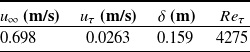
) and, as a result of the inertia carried by the liquid, it bends, reaching the surface of the plate forming an air cavity (see figure 1; note that the images are rotated to have the cavity at the bottom to match prior bump studies). The morphology of the air cavity formed is such that two distinct regions can be identified from visual observations: an almost stable region upstream (left of the dotted black line in figure 1) that is uniform in the span and a shedding region downstream (right of the dotted black line in figure 1) varying in the span and comprising thin sheets of air (see also supplementary movie 1). Given the higher thickness of the spanwise-uniform region compared with that of the shedding region, the former is expected to impose a much larger perturbation to the incoming flow and thus it will be our focus in this study. With the term cavity, we will then refer to the upstream, spanwise-uniform region of the air cavity in what follows.
$62\;\mathrm{l/min}$
) and, as a result of the inertia carried by the liquid, it bends, reaching the surface of the plate forming an air cavity (see figure 1; note that the images are rotated to have the cavity at the bottom to match prior bump studies). The morphology of the air cavity formed is such that two distinct regions can be identified from visual observations: an almost stable region upstream (left of the dotted black line in figure 1) that is uniform in the span and a shedding region downstream (right of the dotted black line in figure 1) varying in the span and comprising thin sheets of air (see also supplementary movie 1). Given the higher thickness of the spanwise-uniform region compared with that of the shedding region, the former is expected to impose a much larger perturbation to the incoming flow and thus it will be our focus in this study. With the term cavity, we will then refer to the upstream, spanwise-uniform region of the air cavity in what follows.
Schematic of the experimental set-up (left). The laser illuminated field of view is shown in green. The cavity (in white) shown upside down in line with the flow geometry encountered in solid bump flows. The cavity’s main geometrical characteristics, ( $t_{max}$
and
$t_{max}$
and $\overline {c}$
(chord length)) are schematically shown in front and bottom views. Two distinct regions can be identified (separated by a dotted black line): an approximately stable spanwise-uniform region upstream and an unstable shedding region downstream. An actual image of the cavity (front view) is also shown on the right. Flow is from left to right. Gravity (g) is from bottom to top.
$\overline {c}$
(chord length)) are schematically shown in front and bottom views. Two distinct regions can be identified (separated by a dotted black line): an approximately stable spanwise-uniform region upstream and an unstable shedding region downstream. An actual image of the cavity (front view) is also shown on the right. Flow is from left to right. Gravity (g) is from bottom to top.
The behaviour of the TBL in the presence of the air cavity is studied using planar PIV in a streamwise–wall-normal plane. The flow is seeded with $15\; \mathrm{\mu m}$
hollow glass spheres that are illuminated by a Litron dual-cavity Nd-YAG laser. Two LaVision Imager sCMOS CLHS cameras (
$15\; \mathrm{\mu m}$
hollow glass spheres that are illuminated by a Litron dual-cavity Nd-YAG laser. Two LaVision Imager sCMOS CLHS cameras ( $5\;\mathrm{Mpix}$
,
$5\;\mathrm{Mpix}$
, $16$
-bit) are used to capture the particle images, placed in a side-by-side configuration, each of them fitted with Nikkor objectives of focal length
$16$
-bit) are used to capture the particle images, placed in a side-by-side configuration, each of them fitted with Nikkor objectives of focal length $105\;\mathrm{mm}$
. The resulting magnification is approximately
$105\;\mathrm{mm}$
. The resulting magnification is approximately $11.8\;\mathrm{pix}/\mathrm{mm}$
and the combined field of view extents
$11.8\;\mathrm{pix}/\mathrm{mm}$
and the combined field of view extents $2.87\delta \times 1.35\delta$
in
$2.87\delta \times 1.35\delta$
in $x$
and
$x$
and $y$
, respectively. A total of
$y$
, respectively. A total of $2500$
uncorrelated image pairs are acquired at a frequency of
$2500$
uncorrelated image pairs are acquired at a frequency of $3\;\mathrm{Hz}$
and subsequently processed using Davis
$3\;\mathrm{Hz}$
and subsequently processed using Davis $10.1.2$
, following a multi-pass approach, with a final window size of
$10.1.2$
, following a multi-pass approach, with a final window size of $48\times 48\; \mathrm{pix}$
and an overlap of
$48\times 48\; \mathrm{pix}$
and an overlap of $50\;\%$
. The resulting final vector spacing is
$50\;\%$
. The resulting final vector spacing is $2\;\mathrm{mm}$
(
$2\;\mathrm{mm}$
( $\Delta l^+ = 52.6$
in viscous units).
$\Delta l^+ = 52.6$
in viscous units).
3. Results and discussion
3.1. Baseline turbulent boundary layer characteristics
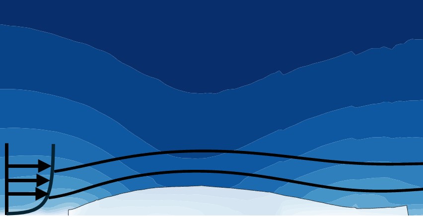
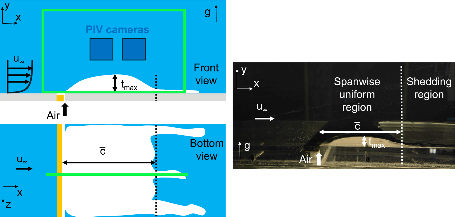
The incoming liquid TBL developing over the wall is first characterised. This is done in the absence of air injection. The presence of the latter was found to impose an upstream APG on the incoming TBL (Anand Reference Anand2021). Therefore, to avoid any complications while comparing the behaviour of the TBL over the cavity with respect to the baseline case (over the wall), we characterise the incoming TBL without the cavity. The inner-normalised mean streamwise velocity and root-mean-square (r.m.s.) streamwise turbulent velocity fluctuations of the baseline TBL are shown in figure 2. In comparison with laser Doppler anemometry (LDA) measurements of DeGraaff & Eaton (Reference DeGraaff and Eaton2000) at comparable Reynolds number, the logarithmic behaviour in the present incoming TBL is not strictly canonical. The absence of a well-formed wake can be explained as a result of a free stream that is more noisy than expected. The underestimation in the r.m.s. streamwise velocity fluctuations observed here compared with the LDA measurements can be explained due to the relatively large interrogation areas employed. The incoming TBL in the present study is not a strictly canonical ZPG TBL as seen in the shortened log region and a mild FPG present due to TBL development ( $K \approx 3\times 10^{-9}$
), the latter, however, much lower compared with the local FPG imposed on the windward side of the cavity (see discussion in section 3.3). Although sufficiently different global incoming TBL conditions such as
$K \approx 3\times 10^{-9}$
), the latter, however, much lower compared with the local FPG imposed on the windward side of the cavity (see discussion in section 3.3). Although sufficiently different global incoming TBL conditions such as $\delta$
and
$\delta$
and $u_{\infty }$
are shown to affect the air cavity characteristics (Nikolaidou et al. Reference Nikolaidou, Laskari, van Terwisga and Poelma2024), here, we focus on the relative TBL changes. Thus, some deviations from canonicality are not expected to affect the general trends discussed here. This is further supported by the
$u_{\infty }$
are shown to affect the air cavity characteristics (Nikolaidou et al. Reference Nikolaidou, Laskari, van Terwisga and Poelma2024), here, we focus on the relative TBL changes. Thus, some deviations from canonicality are not expected to affect the general trends discussed here. This is further supported by the $\delta /t_{max} = 3$
case added for comparison in what follows (see section 3.3).
$\delta /t_{max} = 3$
case added for comparison in what follows (see section 3.3).
Inner-normalised (a) mean streamwise velocity and (b) streamwise velocity intensities for the baseline TBL. Also shown is reference data using LDA at comparable friction Reynolds number ( ${Re}_{\tau}$
) by DeGraaff & Eaton (Reference DeGraaff and Eaton2000).
${Re}_{\tau}$
) by DeGraaff & Eaton (Reference DeGraaff and Eaton2000).
3.2. Air cavity identification
As discussed in section 1, in TBL flows over solid bumps, the shape of the bump, and in particular its height and length, have been observed to influence the development of the TBL (Baskaran et al. Reference Baskaran, Smits and Joubert1987; Webster et al. Reference Webster, DeGraff and Eaton1996). Given the similarity in geometry of the spanwise-uniform region of the cavity with solid bumps in the literature, the shape of the cavity is then also expected to influence the development of the incoming TBL. Therefore, before studying the behaviour of the TBL over the cavity and comparing the flow development with previous solid bump studies, the time-averaged geometry of the cavity needs to be identified and characterised. To this end, an identification technique based on the thresholding of correlation values obtained after image post-processing was employed.
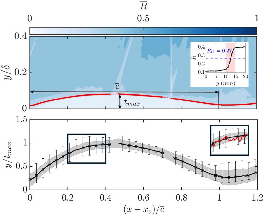
Top: contour of mean correlation map $\overline {R}$
along with the mean cavity identified (in red). Here,
$\overline {R}$
along with the mean cavity identified (in red). Here, $\overline {c}$
is the chord length,
$\overline {c}$
is the chord length, $t_{max}$
is the maximum thickness of the mean cavity and
$t_{max}$
is the maximum thickness of the mean cavity and $x_{o}$
is the leading edge of the mean cavity. Inset: variation of
$x_{o}$
is the leading edge of the mean cavity. Inset: variation of $\overline {R}$
with wall-normal distance at the streamwise location of
$\overline {R}$
with wall-normal distance at the streamwise location of $t_{max}$
(
$t_{max}$
( $\overline {R}_{th}$
: correlation threshold chosen to identify the cavity). Bottom: mean cavity interface (solid black line) with r.m.s. fluctuations of the cavity thickness along the length of the cavity (shaded grey region). Error bars depict the uncertainties in the identification technique. Inset: example of an instantaneous cavity interface detected (in red). See also supplementary movie 1.
$\overline {R}_{th}$
: correlation threshold chosen to identify the cavity). Bottom: mean cavity interface (solid black line) with r.m.s. fluctuations of the cavity thickness along the length of the cavity (shaded grey region). Error bars depict the uncertainties in the identification technique. Inset: example of an instantaneous cavity interface detected (in red). See also supplementary movie 1.
The instantaneous correlation values are obtained through a PIV routine following a multi-pass approach, with a final window size of $24\times 24\;\mathrm{pix}$
and an overlap of
$24\times 24\;\mathrm{pix}$
and an overlap of $50\;\%$
(see figure 3). A smaller final window size (higher spatial resolution) than the one applied to acquire the velocity fields allowed a more accurate estimate of the air–water interface, and therefore the cavity thickness and length through the correlation values. It was, however, found to be too noisy for velocity estimates; hence, a lower resolution final interrogation window was used there (see section 2). A threshold to identify instantaneous geometries of the cavity is obtained using the time-averaged correlation map (figure 3 top). We exploit the fact that correlation values within the cavity should be inherently low compared with the surrounding liquid as there are no tracer particles to correlate with, while patterns within the cavity region (e.g. reflections) also varied significantly between frames and thus did not correlate. This leads to a sharp gradient in correlation between cavity and flow, clearly delineated in the time-averaged map (
$50\;\%$
(see figure 3). A smaller final window size (higher spatial resolution) than the one applied to acquire the velocity fields allowed a more accurate estimate of the air–water interface, and therefore the cavity thickness and length through the correlation values. It was, however, found to be too noisy for velocity estimates; hence, a lower resolution final interrogation window was used there (see section 2). A threshold to identify instantaneous geometries of the cavity is obtained using the time-averaged correlation map (figure 3 top). We exploit the fact that correlation values within the cavity should be inherently low compared with the surrounding liquid as there are no tracer particles to correlate with, while patterns within the cavity region (e.g. reflections) also varied significantly between frames and thus did not correlate. This leads to a sharp gradient in correlation between cavity and flow, clearly delineated in the time-averaged map ( $\overline {R}$
, see inset of figure 3 top). Given the fact that the cavity interface can lie anywhere within this gradient (in the range of
$\overline {R}$
, see inset of figure 3 top). Given the fact that the cavity interface can lie anywhere within this gradient (in the range of $0.15\lt \overline {R}\lt 0.40$
: see shaded red area in inset of figure 3 top), an average of
$0.15\lt \overline {R}\lt 0.40$
: see shaded red area in inset of figure 3 top), an average of $\overline {R}$
in this region is identified as a representative threshold (
$\overline {R}$
in this region is identified as a representative threshold ( $\overline {R}_{th}=0.27$
). This results in an uncertainty (error bars in figure 3 bottom) in the location of the cavity interface of approximately
$\overline {R}_{th}=0.27$
). This results in an uncertainty (error bars in figure 3 bottom) in the location of the cavity interface of approximately $\pm 2\;\mathrm{mm}$
along its length and dominates any spatial resolution effects. Regardless, the chosen threshold does not affect the analysis in the trends discussed later. This threshold is then applied to every image to detect the instantaneous cavity shape, which is found to match relatively well with visual inspection of the raw images (see supplementary movie 1). The mean air–water interface is then obtained by averaging over these instantaneous realisations; comparison with the mean directly identified from the time-averaged correlation map (Nikolaidou et al. Reference Nikolaidou, Laskari, van Terwisga and Poelma2024), yields similar results (
$\pm 2\;\mathrm{mm}$
along its length and dominates any spatial resolution effects. Regardless, the chosen threshold does not affect the analysis in the trends discussed later. This threshold is then applied to every image to detect the instantaneous cavity shape, which is found to match relatively well with visual inspection of the raw images (see supplementary movie 1). The mean air–water interface is then obtained by averaging over these instantaneous realisations; comparison with the mean directly identified from the time-averaged correlation map (Nikolaidou et al. Reference Nikolaidou, Laskari, van Terwisga and Poelma2024), yields similar results ( $\lt 1\;\mathrm{mm}$
difference). The discontinuities observed in the detected interface (figure 3, e.g. near the
$\lt 1\;\mathrm{mm}$
difference). The discontinuities observed in the detected interface (figure 3, e.g. near the $\overline {c}$
label) are due to light path obstructions in the raw particle images. The smoothness of the rest of the field, however, allowed interpolation for the mean shape in these locations.
$\overline {c}$
label) are due to light path obstructions in the raw particle images. The smoothness of the rest of the field, however, allowed interpolation for the mean shape in these locations.
The mean cavity shape reveals a well-defined asymmetric bump-like geometry at the spanwise-uniform part of the cavity upstream (also supported by visual observations). The highly dynamic nature of the shedding region of the cavity downstream, its limited thickness and significantly lower correlation gradients, did not allow for a valid identification of the same. The maximum thickness and chord length of the mean cavity were found to be $t_{max} = 13.2\pm 2\;\mathrm{mm}$
and
$t_{max} = 13.2\pm 2\;\mathrm{mm}$
and $\overline {c} = 143\pm 2\;\mathrm{mm}$
, respectively. The ratio of the incoming boundary layer thickness to the maximum thickness of the cavity was found to be
$\overline {c} = 143\pm 2\;\mathrm{mm}$
, respectively. The ratio of the incoming boundary layer thickness to the maximum thickness of the cavity was found to be $\delta /t_{max} = 12$
, which is considerably higher than the ratios encountered in the solid bump studies of Baskaran et al. (Reference Baskaran, Smits and Joubert1987) and Webster et al. (Reference Webster, DeGraff and Eaton1996) (
$\delta /t_{max} = 12$
, which is considerably higher than the ratios encountered in the solid bump studies of Baskaran et al. (Reference Baskaran, Smits and Joubert1987) and Webster et al. (Reference Webster, DeGraff and Eaton1996) ( $\delta /h = 0.25$
and
$\delta /h = 0.25$
and $\delta /h = 1.5$
, respectively).
$\delta /h = 1.5$
, respectively).
Unlike solid bumps for which length and thickness are constant, these parameters vary in space and time for the air cavity studied here. However, when looking at the instantaneous cavity shapes (see supplementary movie 1) and r.m.s. fluctuations of the cavity thickness across its length (grey shaded region around the mean cavity in figure 3 bottom), there are no significant deviations of the cavity from a bump-like geometry. The r.m.s. deviation of the maximum thickness and chord length of the cavity detected (approximately $5.8\;\mathrm{\%}$
and
$5.8\;\mathrm{\%}$
and $5.2\;\mathrm{\%}$
compared with the mean, respectively), however, are lower than the estimated experimental uncertainty (approximately
$5.2\;\mathrm{\%}$
compared with the mean, respectively), however, are lower than the estimated experimental uncertainty (approximately $7\;\mathrm{\%}$
of
$7\;\mathrm{\%}$
of $t_{max}$
) (see inset of figure 3 bottom and figure 12 in the Appendix), and as such no conclusions can be drawn on it. As detailed analysis of small-scale features (capillary waves or ripples) of the gas–liquid interface lies beyond this study’s scope, we will use the average cavity shape in the analysis that follows. Measurement techniques tailored to interfacial physics would better capture these instantaneous features (for example Gomit et al. (Reference Gomit, Chatellier and David2022); van Meerkerk et al. (Reference van Meerkerk, Poelma and Westerweel2020)).
$t_{max}$
) (see inset of figure 3 bottom and figure 12 in the Appendix), and as such no conclusions can be drawn on it. As detailed analysis of small-scale features (capillary waves or ripples) of the gas–liquid interface lies beyond this study’s scope, we will use the average cavity shape in the analysis that follows. Measurement techniques tailored to interfacial physics would better capture these instantaneous features (for example Gomit et al. (Reference Gomit, Chatellier and David2022); van Meerkerk et al. (Reference van Meerkerk, Poelma and Westerweel2020)).
With the mean cavity geometry defined, the flow behaviour around it can then be analysed. In what follows, a modified coordinate system based on the mean cavity geometry will be employed. The normalised streamwise coordinate is defined as $x' = (x-x_{o})/\overline {c}$
, with
$x' = (x-x_{o})/\overline {c}$
, with $x_{o}$
being the leading edge of the cavity. Using the instantaneous cavity lengths instead of
$x_{o}$
being the leading edge of the cavity. Using the instantaneous cavity lengths instead of $\overline {c}$
did not alter any of the presented results, corroborated by no significant deviations of the instantaneous cavity lengths from the mean (approximately
$\overline {c}$
did not alter any of the presented results, corroborated by no significant deviations of the instantaneous cavity lengths from the mean (approximately $5.2\;\mathrm{\%}$
). Thus, normalisation based on
$5.2\;\mathrm{\%}$
). Thus, normalisation based on $\overline {c}$
was chosen for the analysis. The wall-normal coordinate,
$\overline {c}$
was chosen for the analysis. The wall-normal coordinate, $y'$
is normalised with
$y'$
is normalised with $\delta$
, and is defined with its zero location based on the mean interface height, and maintained normal to the flat plate at the interface positions, the latter employed owing to a relatively large
$\delta$
, and is defined with its zero location based on the mean interface height, and maintained normal to the flat plate at the interface positions, the latter employed owing to a relatively large $\delta /t_{max}$
(and minimal streamline curvature) (Webster et al. Reference Webster, DeGraff and Eaton1996).
$\delta /t_{max}$
(and minimal streamline curvature) (Webster et al. Reference Webster, DeGraff and Eaton1996).
3.3. Turbulence statistics
The mean streamwise velocity field clearly illustrates that the incoming TBL experiences an alternating streamwise pressure gradient over the length of the cavity (figure 4). The TBL first experiences an APG, as indicated by the moderate elevation of the contour lines at the leading edge of the cavity ( $x'=0$
). The flow then accelerates around the apex of the cavity, indicating a FPG, while it decelerates past the apex due to an APG, with no indication of incipient separation. To get some further insight on the influence of the cavity on the TBL, the streamwise variation of the local boundary layer thickness
$x'=0$
). The flow then accelerates around the apex of the cavity, indicating a FPG, while it decelerates past the apex due to an APG, with no indication of incipient separation. To get some further insight on the influence of the cavity on the TBL, the streamwise variation of the local boundary layer thickness $\delta$
is also computed and compared with the solid bump study by Baskaran et al. (Reference Baskaran, Smits and Joubert1987). Estimation of
$\delta$
is also computed and compared with the solid bump study by Baskaran et al. (Reference Baskaran, Smits and Joubert1987). Estimation of $\delta$
in non-equilibrium TBLs (for example subjected to pressure gradients) is typically difficult as the mean velocities and wall-normal gradients beyond the boundary layer edge do not exactly go to zero (see also the discussion in Vinuesa et al. (Reference Vinuesa, Bobke, Örlü and Schlatter2016)). Here, the local boundary layer thickness is defined as the average wall-normal location where the streamwise, wall-normal and Reynolds shear stresses approach an approximately constant value in the free stream. A similar technique using turbulent quantities to identify the boundary layer thickness in open channel flows was also used by Das et al. (Reference Das, Balachander and Barron2022).
$\delta$
in non-equilibrium TBLs (for example subjected to pressure gradients) is typically difficult as the mean velocities and wall-normal gradients beyond the boundary layer edge do not exactly go to zero (see also the discussion in Vinuesa et al. (Reference Vinuesa, Bobke, Örlü and Schlatter2016)). Here, the local boundary layer thickness is defined as the average wall-normal location where the streamwise, wall-normal and Reynolds shear stresses approach an approximately constant value in the free stream. A similar technique using turbulent quantities to identify the boundary layer thickness in open channel flows was also used by Das et al. (Reference Das, Balachander and Barron2022).
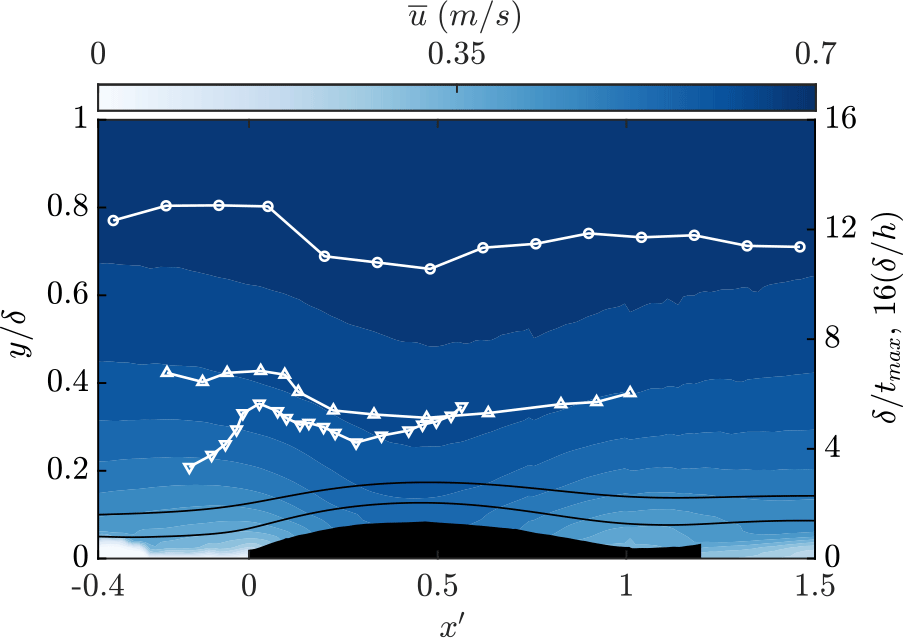
Mean streamwise velocity contours with some streamlines (solid black lines); $x'=0$
is the leading edge of the cavity where
$x'=0$
is the leading edge of the cavity where $x' = (x-x_{o})/\overline {c}$
. The local
$x' = (x-x_{o})/\overline {c}$
. The local $\delta$
from the present study (circles;
$\delta$
from the present study (circles; $\delta /t_{max}=12$
) is compared with that over a thicker air cavity (Anand (Reference Anand2021): upward-pointing triangles;
$\delta /t_{max}=12$
) is compared with that over a thicker air cavity (Anand (Reference Anand2021): upward-pointing triangles; $\delta /t_{max}=7$
), both normalised by the maximum cavity thickness
$\delta /t_{max}=7$
), both normalised by the maximum cavity thickness $t_{max}$
, and that over a solid bump (Baskaran et al. (Reference Baskaran, Smits and Joubert1987): downward-pointing triangles;
$t_{max}$
, and that over a solid bump (Baskaran et al. (Reference Baskaran, Smits and Joubert1987): downward-pointing triangles; $\delta /h=0.25$
), normalised by the maximum bump height
$\delta /h=0.25$
), normalised by the maximum bump height $h$
. Flow is from left to right.
$h$
. Flow is from left to right.
The streamwise variation of $\delta$
in the present study (see figure 4) follows the trend set by alternating pressure gradients discussed previously: a relatively small growth around the leading edge of the cavity due to an APG, followed by a thinning over the windward side of the cavity until the apex due to a FPG and finally a thickening over the leeward side of the cavity due to an APG. This is also in line with trends observed in the studies of Anand (Reference Anand2021) and Baskaran et al. (Reference Baskaran, Smits and Joubert1987) (air cavity and solid bump, respectively). The TBL here (and in Anand (Reference Anand2021)), was found to not separate at the leeward side of the cavity under APG conditions, whereas incipient separation was observed in Baskaran et al. (Reference Baskaran, Smits and Joubert1987) at the leeward side of the solid bump. This is due to the marked difference of the
$\delta$
in the present study (see figure 4) follows the trend set by alternating pressure gradients discussed previously: a relatively small growth around the leading edge of the cavity due to an APG, followed by a thinning over the windward side of the cavity until the apex due to a FPG and finally a thickening over the leeward side of the cavity due to an APG. This is also in line with trends observed in the studies of Anand (Reference Anand2021) and Baskaran et al. (Reference Baskaran, Smits and Joubert1987) (air cavity and solid bump, respectively). The TBL here (and in Anand (Reference Anand2021)), was found to not separate at the leeward side of the cavity under APG conditions, whereas incipient separation was observed in Baskaran et al. (Reference Baskaran, Smits and Joubert1987) at the leeward side of the solid bump. This is due to the marked difference of the $\delta /t_{max}$
(
$\delta /t_{max}$
( $\delta /h$
) ratio between the three studies, with low values of this ratio typically leading to separation under APG conditions. We note that the presence of a free-slip boundary condition (at the cavity) can delay flow separation, as has been observed in the numerical study of flow over a Gaussian bump (Ceccacci et al. Reference Ceccacci, Calabretto, Thomas and Denier2022). However, the
$\delta /h$
) ratio between the three studies, with low values of this ratio typically leading to separation under APG conditions. We note that the presence of a free-slip boundary condition (at the cavity) can delay flow separation, as has been observed in the numerical study of flow over a Gaussian bump (Ceccacci et al. Reference Ceccacci, Calabretto, Thomas and Denier2022). However, the $\delta /t_{max}$
ratio in the current study is higher than the
$\delta /t_{max}$
ratio in the current study is higher than the $\delta /h = 1.5$
used by Webster et al. (Reference Webster, DeGraff and Eaton1996) for a solid bump, where no TBL separation occurred. Thus, the present ratio is expected to be sufficiently high to prevent flow separation irrespective of whether the boundary condition at the bump is no slip (solid bump) or free slip (air cavity).
$\delta /h = 1.5$
used by Webster et al. (Reference Webster, DeGraff and Eaton1996) for a solid bump, where no TBL separation occurred. Thus, the present ratio is expected to be sufficiently high to prevent flow separation irrespective of whether the boundary condition at the bump is no slip (solid bump) or free slip (air cavity).
In order to more closely investigate these alternating pressure gradient effects on the TBL across the cavity, the mean velocity and turbulent stresses profiles are evaluated next, at selected streamwise locations. The profiles have been normalised by local outer units, that is, using the local $\delta$
and
$\delta$
and $U_{\infty }$
at each streamwise location. As mentioned previously, all profiles are evaluated over the cavity, thus using the local coordinate system
$U_{\infty }$
at each streamwise location. As mentioned previously, all profiles are evaluated over the cavity, thus using the local coordinate system $(x', y')$
.
$(x', y')$
.
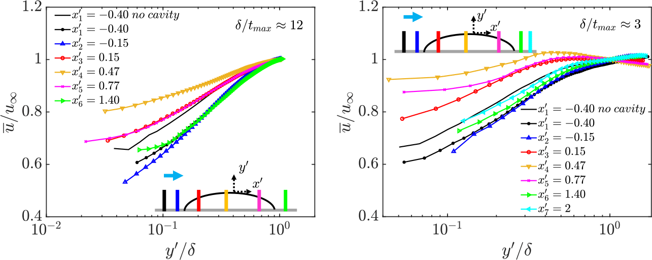
Variation of mean streamwise velocity (markers) for $\delta /t_{max}\approx 12$
(left) and
$\delta /t_{max}\approx 12$
(left) and $\delta /t_{max}\approx 3$
(right) across different streamwise locations over the cavity, normalised with local outer units. Colours represent different streamwise locations along the cavity, as shown in the inset. The profile at
$\delta /t_{max}\approx 3$
(right) across different streamwise locations over the cavity, normalised with local outer units. Colours represent different streamwise locations along the cavity, as shown in the inset. The profile at $x'_{1}$
without a cavity is denoted with a black line. Flow is from left to right.
$x'_{1}$
without a cavity is denoted with a black line. Flow is from left to right.
The mean velocity profiles at different streamwise locations exhibit deviations in the inner and logarithmic regions compared with the baseline case (figure 5, left). An upstream influence imposed by the leading edge of the cavity on the incoming boundary layer can be observed at streamwise locations $x_{1}'$
and
$x_{1}'$
and $x'_{2}$
, where an APG causes a deficit in the mean velocity compared with when no cavity is present. This influence has been estimated to last until approximately
$x'_{2}$
, where an APG causes a deficit in the mean velocity compared with when no cavity is present. This influence has been estimated to last until approximately $0.9\delta$
upstream of the leading edge of the cavity, beyond which the TBL relaxed to its baseline state (Anand Reference Anand2021; Nikolaidou et al. Reference Nikolaidou, Laskari, van Terwisga and Poelma2024). Over the windward side of the cavity, a switch in the pressure gradient to a favourable one causes the TBL to accelerate, as highlighted by the increase in mean streamwise velocity until the apex (approximately
$0.9\delta$
upstream of the leading edge of the cavity, beyond which the TBL relaxed to its baseline state (Anand Reference Anand2021; Nikolaidou et al. Reference Nikolaidou, Laskari, van Terwisga and Poelma2024). Over the windward side of the cavity, a switch in the pressure gradient to a favourable one causes the TBL to accelerate, as highlighted by the increase in mean streamwise velocity until the apex (approximately $x'_{4}$
). The profiles display a systematic deviation from log-law behaviour, which was also reported by Narasimha & Sreenivasan (Reference Narasimha and Sreenivasan1979) in strongly accelerating flows as due to the stabilising effects of FPGs. At the leeward side of the cavity (
$x'_{4}$
). The profiles display a systematic deviation from log-law behaviour, which was also reported by Narasimha & Sreenivasan (Reference Narasimha and Sreenivasan1979) in strongly accelerating flows as due to the stabilising effects of FPGs. At the leeward side of the cavity ( $x'_{5}$
), the boundary layer decelerates compared with the mean velocity at
$x'_{5}$
), the boundary layer decelerates compared with the mean velocity at $x_{4}'$
due to an APG, however, it is still faster than the incoming flow due to the upstream FPG. Overall, the mean velocity profile variation over the cavity follows the trend set by the alternating streamwise pressure gradients, in line with the boundary layer thickness variations discussed previously (see figure 4). In an independent experimental campaign in the same set-up, but with the air injector located further upstream such that a relatively low
$x_{4}'$
due to an APG, however, it is still faster than the incoming flow due to the upstream FPG. Overall, the mean velocity profile variation over the cavity follows the trend set by the alternating streamwise pressure gradients, in line with the boundary layer thickness variations discussed previously (see figure 4). In an independent experimental campaign in the same set-up, but with the air injector located further upstream such that a relatively low $\delta /t_{max} \approx 3$
was achieved (Nikolaidou et al. Reference Nikolaidou, Laskari, van Terwisga and Poelma2024), similar trends in the mean streamwise velocity over the cavity were observed (figure 5 right), again with no TBL separation. The recovery of the TBL at
$\delta /t_{max} \approx 3$
was achieved (Nikolaidou et al. Reference Nikolaidou, Laskari, van Terwisga and Poelma2024), similar trends in the mean streamwise velocity over the cavity were observed (figure 5 right), again with no TBL separation. The recovery of the TBL at $x'_{6}$
back to its state upstream of the cavity (at
$x'_{6}$
back to its state upstream of the cavity (at $x'_{1}$
), occurs within one
$x'_{1}$
), occurs within one $\delta$
from the trailing edge of the cavity. Further downstream, the return of the TBL to its baseline state (at
$\delta$
from the trailing edge of the cavity. Further downstream, the return of the TBL to its baseline state (at $x'_{1}$
without a cavity) occurs within a cavity length (
$x'_{1}$
without a cavity) occurs within a cavity length ( $\approx 3\delta$
) from the trailing edge of the cavity (figure 5, right).
$\approx 3\delta$
) from the trailing edge of the cavity (figure 5, right).
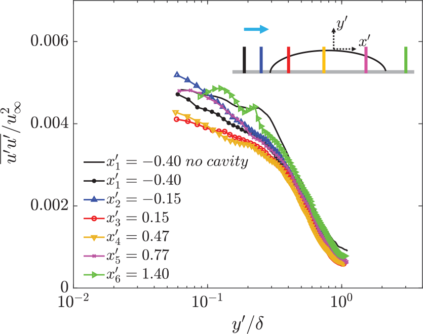
Variation of the streamwise normal stress $\overline {u'u'}$
across different streamwise locations over the cavity (markers) normalised with local outer units. Colours represent different streamwise locations along the cavity, as shown in the inset. The profile at
$\overline {u'u'}$
across different streamwise locations over the cavity (markers) normalised with local outer units. Colours represent different streamwise locations along the cavity, as shown in the inset. The profile at $x'_{1}$
, when no cavity was present, is denoted with a black line. Flow is from left to right.
$x'_{1}$
, when no cavity was present, is denoted with a black line. Flow is from left to right.
Variation of the wall-normal stress $\overline {v'v'}$
across different streamwise positions of the cavity (markers) normalised in local outer units. Colours represent different streamwise locations along the cavity, as shown in the inset. The profile at
$\overline {v'v'}$
across different streamwise positions of the cavity (markers) normalised in local outer units. Colours represent different streamwise locations along the cavity, as shown in the inset. The profile at $x'_{1}$
, when no cavity was present, is denoted with a black line. Flow is from left to right.
$x'_{1}$
, when no cavity was present, is denoted with a black line. Flow is from left to right.

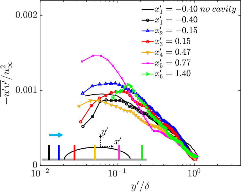
Variation of the Reynolds shear stress $-\overline {u'v'}$
across different streamwise positions of the cavity (lines with markers) normalised in local outer units. Colours represent different streamwise locations along the cavity, as shown in the inset. The profile at
$-\overline {u'v'}$
across different streamwise positions of the cavity (lines with markers) normalised in local outer units. Colours represent different streamwise locations along the cavity, as shown in the inset. The profile at $x'_{1}$
, when no cavity was present, is denoted with a black line. Flow is from left to right.
$x'_{1}$
, when no cavity was present, is denoted with a black line. Flow is from left to right.
The variation of the streamwise normal ( $\overline {u'u'}$
, figure 6), wall-normal (
$\overline {u'u'}$
, figure 6), wall-normal ( $\overline {v'v'}$
, figure 7) and Reynolds shear stress profiles (-
$\overline {v'v'}$
, figure 7) and Reynolds shear stress profiles (- $\overline {u'v'}$
, figure 8) across the length of the cavity are investigated next. Higher than anticipated reflections from the cavity did not allow for in-depth analysis of the stresses for the prior independent experimental campaign where
$\overline {u'v'}$
, figure 8) across the length of the cavity are investigated next. Higher than anticipated reflections from the cavity did not allow for in-depth analysis of the stresses for the prior independent experimental campaign where $\delta /t_{max}\approx 3$
(although qualitatively similar behaviour was observed overall) and as such will not be included in the forthcoming discussion. The strongest variations as compared with the no cavity case are observed in the
$\delta /t_{max}\approx 3$
(although qualitatively similar behaviour was observed overall) and as such will not be included in the forthcoming discussion. The strongest variations as compared with the no cavity case are observed in the $\overline {v'v'}$
and
$\overline {v'v'}$
and $-\overline {u'v'}$
profiles, and they extend throughout the majority of the TBL height. Variations in
$-\overline {u'v'}$
profiles, and they extend throughout the majority of the TBL height. Variations in $\overline {u'u'}$
, on the other hand, are less pronounced (figure 6) and are restricted to
$\overline {u'u'}$
, on the other hand, are less pronounced (figure 6) and are restricted to $y' \lt 0.4\delta$
, with the rest of the outer region showing a near collapse under outer scaling. Furthermore, the stress profiles do not exhibit “knee” points, which are typical markers for an internal layer triggered within the TBL (Balin & Jansen Reference Balin and Jansen2021; Parthasarathy & Saxton-Fox Reference Parthasarathy and Saxton-Fox2023; Webster et al. Reference Webster, DeGraff and Eaton1996) (see section 1 ). Internal layers have been reported to be formed in TBLs subjected to relatively strong favourable–adverse pressure gradients (quantified by
$y' \lt 0.4\delta$
, with the rest of the outer region showing a near collapse under outer scaling. Furthermore, the stress profiles do not exhibit “knee” points, which are typical markers for an internal layer triggered within the TBL (Balin & Jansen Reference Balin and Jansen2021; Parthasarathy & Saxton-Fox Reference Parthasarathy and Saxton-Fox2023; Webster et al. Reference Webster, DeGraff and Eaton1996) (see section 1 ). Internal layers have been reported to be formed in TBLs subjected to relatively strong favourable–adverse pressure gradients (quantified by $K\gtrsim 2\times 10^{-6}$
) typically imposed at low
$K\gtrsim 2\times 10^{-6}$
) typically imposed at low $\delta /h$
ratios (Parthasarathy & Saxton-Fox Reference Parthasarathy and Saxton-Fox2023); however, internal layers are not expected to be triggered in the TBL here (
$\delta /h$
ratios (Parthasarathy & Saxton-Fox Reference Parthasarathy and Saxton-Fox2023); however, internal layers are not expected to be triggered in the TBL here ( $K\approx 0.3\times 10^{-6}$
,
$K\approx 0.3\times 10^{-6}$
, $\delta /t_{max}= 12$
).
$\delta /t_{max}= 12$
).
As the TBL moves over the windward side of the cavity where it is subjected to a FPG, a suppression in $\overline {u'u'}$
and
$\overline {u'u'}$
and $-\overline {u'v'}$
profiles throughout the boundary layer is observed as expected (Volino Reference Volino2020). However,
$-\overline {u'v'}$
profiles throughout the boundary layer is observed as expected (Volino Reference Volino2020). However, $\overline {v'v'}$
exhibits a marked increase below
$\overline {v'v'}$
exhibits a marked increase below $y\approx 0.3\delta$
throughout the length of the cavity (figure 7), even in the region where an attenuation of stresses is expected due to a FPG (station
$y\approx 0.3\delta$
throughout the length of the cavity (figure 7), even in the region where an attenuation of stresses is expected due to a FPG (station $x'_{3}$
). In addition, the general shape of the
$x'_{3}$
). In addition, the general shape of the $\overline {v'v'}$
profiles over the length of the cavity appears to be largely different in character compared with its state at
$\overline {v'v'}$
profiles over the length of the cavity appears to be largely different in character compared with its state at $x'_1$
and
$x'_1$
and $x'_{2}$
. The amplification of
$x'_{2}$
. The amplification of $\overline {v'v'}$
at
$\overline {v'v'}$
at $x'_{3}$
and
$x'_{3}$
and $x'_{4}$
relative to
$x'_{4}$
relative to $x'_{2}$
, does not follow the expected trend based on the influence of a FPG, the latter which is observed in
$x'_{2}$
, does not follow the expected trend based on the influence of a FPG, the latter which is observed in $\overline {u'u'}$
and
$\overline {u'u'}$
and $-\overline {u'v'}$
. Instead, the vertical momentum induced by the air injection seems to dominate the
$-\overline {u'v'}$
. Instead, the vertical momentum induced by the air injection seems to dominate the $\overline {v'v'}$
profiles overshadowing any potential pressure gradient effects. This behaviour of
$\overline {v'v'}$
profiles overshadowing any potential pressure gradient effects. This behaviour of $\overline {v'v'}$
in addition to a free-slip boundary condition is what sets it apart from solid bump studies. Variations in
$\overline {v'v'}$
in addition to a free-slip boundary condition is what sets it apart from solid bump studies. Variations in $-\overline {u'v'}$
follow the alternating streamwise pressure gradient trend (as observed in
$-\overline {u'v'}$
follow the alternating streamwise pressure gradient trend (as observed in $\overline {u'u'}$
in figure 6), with a notable increase below
$\overline {u'u'}$
in figure 6), with a notable increase below $y\approx 0.3\delta$
at
$y\approx 0.3\delta$
at $x'_5$
compared with
$x'_5$
compared with $x'_3$
and
$x'_3$
and $x'_4$
. This increase can be explained due to the combined effects of the APG imposed by the cavity’s leeward side and the momentum induced by the air injection (reflected in
$x'_4$
. This increase can be explained due to the combined effects of the APG imposed by the cavity’s leeward side and the momentum induced by the air injection (reflected in $\overline {v'v'}$
). A weakening of
$\overline {v'v'}$
). A weakening of $\overline {v'v'}$
and
$\overline {v'v'}$
and $-\overline {u'v'}$
above
$-\overline {u'v'}$
above $y\approx 0.3\delta$
at
$y\approx 0.3\delta$
at $x'_{4}$
and
$x'_{4}$
and $x'_{5}$
is observed relative to the stations over the windward side of the cavity. Weakening of stresses in the outer region has been attributed to effects of convex streamline curvature (Balin & Jansen Reference Balin and Jansen2021; Baskaran et al. Reference Baskaran, Smits and Joubert1987) or a combination of convex streamline curvature and FPG effects (Uzun & Malik Reference Uzun and Malik2021). However, the weakening in
$x'_{5}$
is observed relative to the stations over the windward side of the cavity. Weakening of stresses in the outer region has been attributed to effects of convex streamline curvature (Balin & Jansen Reference Balin and Jansen2021; Baskaran et al. Reference Baskaran, Smits and Joubert1987) or a combination of convex streamline curvature and FPG effects (Uzun & Malik Reference Uzun and Malik2021). However, the weakening in $\overline {v'v'}$
and
$\overline {v'v'}$
and $-\overline {u'v'}$
observed here is not expected to be due to streamline curvature, but is instead solely driven by the effects of FPG. In the solid bump study of Baskaran et al. (Reference Baskaran, Smits and Joubert1987) where
$-\overline {u'v'}$
observed here is not expected to be due to streamline curvature, but is instead solely driven by the effects of FPG. In the solid bump study of Baskaran et al. (Reference Baskaran, Smits and Joubert1987) where $\delta /h = 0.25$
, they noticed a decline in the turbulent stresses in the outer region which was attributed to a prolonged streamline curvature. While in the solid bump study of Webster et al. (Reference Webster, DeGraff and Eaton1996) with
$\delta /h = 0.25$
, they noticed a decline in the turbulent stresses in the outer region which was attributed to a prolonged streamline curvature. While in the solid bump study of Webster et al. (Reference Webster, DeGraff and Eaton1996) with $\delta /h = 1.5$
, only mild variations were observed in the outer region of the stresses, which was attributed to a minimal impact of streamline curvature. In addition, Anand (Reference Anand2021) reported a near collapse above
$\delta /h = 1.5$
, only mild variations were observed in the outer region of the stresses, which was attributed to a minimal impact of streamline curvature. In addition, Anand (Reference Anand2021) reported a near collapse above $y\approx 0.4\delta$
in the
$y\approx 0.4\delta$
in the $\overline {u'u'}$
and
$\overline {u'u'}$
and $-\overline {u'v'}$
profiles across different streamwise positions along the cavity for
$-\overline {u'v'}$
profiles across different streamwise positions along the cavity for $\delta /t_{max} = 7$
. Therefore, if streamline curvature induced by the shape of cavity was indeed important in the current study, we would expect
$\delta /t_{max} = 7$
. Therefore, if streamline curvature induced by the shape of cavity was indeed important in the current study, we would expect $\overline {u'u'}$
to show a decrease (similar to
$\overline {u'u'}$
to show a decrease (similar to $\overline {v'v'}$
and
$\overline {v'v'}$
and $-\overline {u'v'}$
) at higher distances from the wall (
$-\overline {u'v'}$
) at higher distances from the wall ( $y' \gt 0.4\delta$
). Moreover, at higher
$y' \gt 0.4\delta$
). Moreover, at higher $\delta /t_{max}$
ratios (compared with
$\delta /t_{max}$
ratios (compared with $\delta /h = 1.5$
(Webster et al. Reference Webster, DeGraff and Eaton1996) and
$\delta /h = 1.5$
(Webster et al. Reference Webster, DeGraff and Eaton1996) and $\delta /t_{max} = 7$
(Anand Reference Anand2021); in the current study,
$\delta /t_{max} = 7$
(Anand Reference Anand2021); in the current study, $\delta /t_{max} = 12$
), we would expect streamline curvature effects induced by the shape of the cavity (or a solid bump) to be even less important. Alternating streamwise pressure gradients and air injection are therefore expected to be the dominant perturbations to the incoming TBL in the current study, the latter being more prominent in the windward side of the cavity.
$\delta /t_{max} = 12$
), we would expect streamline curvature effects induced by the shape of the cavity (or a solid bump) to be even less important. Alternating streamwise pressure gradients and air injection are therefore expected to be the dominant perturbations to the incoming TBL in the current study, the latter being more prominent in the windward side of the cavity.
Up until this point, only single-point statistics of the TBL have been considered, focusing on magnitude variations across $\delta$
due to the presence of the air cavity;
$\delta$
due to the presence of the air cavity; $\overline {v'v'}$
profiles were those impacted the most in both magnitude and overall shape. To further investigate how these variations translate to a change in spatial coherence, two-point correlations of the wall-normal fluctuations (
$\overline {v'v'}$
profiles were those impacted the most in both magnitude and overall shape. To further investigate how these variations translate to a change in spatial coherence, two-point correlations of the wall-normal fluctuations ( $R_{v'v'}$
) were computed (see figure 9 and table 2), at two reference wall-normal locations (
$R_{v'v'}$
) were computed (see figure 9 and table 2), at two reference wall-normal locations ( $y_{ref}=0.1\delta$
and
$y_{ref}=0.1\delta$
and $0.4\delta$
). The extent of
$0.4\delta$
). The extent of $R_{v'v'}$
in the streamwise (
$R_{v'v'}$
in the streamwise ( $L_x$
) and wall-normal direction (
$L_x$
) and wall-normal direction ( $L_y$
), was estimated based on an elliptical fit to
$L_y$
), was estimated based on an elliptical fit to $R_{v'v'}$
at a correlation level of
$R_{v'v'}$
at a correlation level of $0.3$
(Wu & Christensen Reference Wu and Christensen2010). Qualitatively, with no cavity present,
$0.3$
(Wu & Christensen Reference Wu and Christensen2010). Qualitatively, with no cavity present, $R_{v'v'}$
was found to be narrow and elongated in the wall-normal direction (red line contour in figure 9) consistent with previous observations of
$R_{v'v'}$
was found to be narrow and elongated in the wall-normal direction (red line contour in figure 9) consistent with previous observations of $R_{v'v'}$
over smooth walls (Krogstad & Antonia Reference Krogstad and Antonia1994; Wu & Christensen Reference Wu and Christensen2010); the spatial extent of
$R_{v'v'}$
over smooth walls (Krogstad & Antonia Reference Krogstad and Antonia1994; Wu & Christensen Reference Wu and Christensen2010); the spatial extent of $R_{v'v'}$
evaluated at
$R_{v'v'}$
evaluated at $y_{ref}= 0.15\delta$
and
$y_{ref}= 0.15\delta$
and $R_{v'v'} = 0.3$
was found to agree reasonably well with similar estimates in canonical TBLs in the literature (current study:
$R_{v'v'} = 0.3$
was found to agree reasonably well with similar estimates in canonical TBLs in the literature (current study: $L_x=0.11\delta$
and
$L_x=0.11\delta$
and $L_y= 0.14\delta$
; Wu & Christensen (Reference Wu and Christensen2010):
$L_y= 0.14\delta$
; Wu & Christensen (Reference Wu and Christensen2010): $L_x= 0.16\delta$
and
$L_x= 0.16\delta$
and $L_y= 0.18\delta$
).
$L_y= 0.18\delta$
).
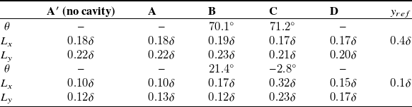
Orientation ( $\theta$
) and extent (
$\theta$
) and extent ( $L_x$
and
$L_x$
and $L_y$
) of
$L_y$
) of $R_{v'v'}$
(at a level of
$R_{v'v'}$
(at a level of $0.3$
, based on figure 9). Note that the streamwise positions chosen (A to D) match those in figure 9 for clarity, while the no cavity case at the most upstream position is also added for comparison (denoted with A′
)
$0.3$
, based on figure 9). Note that the streamwise positions chosen (A to D) match those in figure 9 for clarity, while the no cavity case at the most upstream position is also added for comparison (denoted with A′
)
In the presence of the cavity, the spatial structure of $R_{v'v'}$
undergoes marked changes as the TBL travels over the cavity. This is more prominently observed at
$R_{v'v'}$
undergoes marked changes as the TBL travels over the cavity. This is more prominently observed at $y_{ref}=0.1\delta$
compared with
$y_{ref}=0.1\delta$
compared with $y_{ref}=0.4\delta$
(see figure 9 and bottom row of table 2). The coherence in
$y_{ref}=0.4\delta$
(see figure 9 and bottom row of table 2). The coherence in $R_{v'v'}$
at
$R_{v'v'}$
at $y_{ref}=0.4\delta$
remains relatively similar at all streamwise regions examined with no significant changes in the spatial extent of coherence compared with the baseline case (no cavity present). It should be noted here that this similarity in spatial coherence of
$y_{ref}=0.4\delta$
remains relatively similar at all streamwise regions examined with no significant changes in the spatial extent of coherence compared with the baseline case (no cavity present). It should be noted here that this similarity in spatial coherence of $R_{v'v'}$
at
$R_{v'v'}$
at $y\gt 0.4\delta$
is, however, coupled with marked changes in magnitude, as shown in the intensity profile evolution of
$y\gt 0.4\delta$
is, however, coupled with marked changes in magnitude, as shown in the intensity profile evolution of $v'v'$
over the cavity (see figure 7).
$v'v'$
over the cavity (see figure 7).
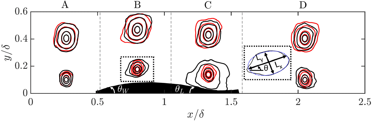
Two-point correlations of wall-normal velocity fluctuations $R_{v'v'}$
at four different streamwise regions (
$R_{v'v'}$
at four different streamwise regions ( $A$
to
$A$
to $D$
) and at two wall-normal locations (
$D$
) and at two wall-normal locations ( $y= 0.1\delta$
and
$y= 0.1\delta$
and $y= 0.4\delta$
), for the cases with (black lines) and without (red lines) the cavity present. Vertical dashed lines demarcate the different streamwise regions where
$y= 0.4\delta$
), for the cases with (black lines) and without (red lines) the cavity present. Vertical dashed lines demarcate the different streamwise regions where $R_{v'v'}$
is computed. Note that the local
$R_{v'v'}$
is computed. Note that the local $\delta$
is used for normalisation. Contour levels used: [
$\delta$
is used for normalisation. Contour levels used: [ $0.3\;0.4\;0.6\;0.8\;1$
]. Inset: illustration of the elliptical fit (blue dash-dotted line) used for the extent (
$0.3\;0.4\;0.6\;0.8\;1$
]. Inset: illustration of the elliptical fit (blue dash-dotted line) used for the extent ( $L_x$
and
$L_x$
and $L_y$
) and orientation (
$L_y$
) and orientation ( $\theta$
) estimates of
$\theta$
) estimates of $R_{v'v'}$
at a
$R_{v'v'}$
at a $0.3$
correlation level (see table 2). Approximate inclinations of the cavity: windward side
$0.3$
correlation level (see table 2). Approximate inclinations of the cavity: windward side $\theta _W \approx 14.3^\circ$
and leeward side
$\theta _W \approx 14.3^\circ$
and leeward side $\theta _L \approx -7.7^\circ$
. Flow is from left to right.
$\theta _L \approx -7.7^\circ$
. Flow is from left to right.
At $y_{ref}=0.1\delta$
, changes to both the aspect ratio and the orientation of
$y_{ref}=0.1\delta$
, changes to both the aspect ratio and the orientation of $R_{v'v'}$
are observed over the cavity (regions
$R_{v'v'}$
are observed over the cavity (regions $B$
and
$B$
and $C$
in figure 9), while just upstream of the leading edge (region
$C$
in figure 9), while just upstream of the leading edge (region $A$
) they are both relatively similar compared with the baseline case. On average, the spatial structures in regions
$A$
) they are both relatively similar compared with the baseline case. On average, the spatial structures in regions $B$
and
$B$
and $C$
are found to approximately follow the inclinations imposed by the cavity. In terms of aspect ratio, at region
$C$
are found to approximately follow the inclinations imposed by the cavity. In terms of aspect ratio, at region $B$
, contours of
$B$
, contours of $R_{v'v'}$
exhibit an increase in the streamwise spatial extent increasing the aspect ratio beyond
$R_{v'v'}$
exhibit an increase in the streamwise spatial extent increasing the aspect ratio beyond $1$
. This can be attributed to the acceleration imposed by the FPG at the windward side of the cavity: a similar increase in the spatial extent of
$1$
. This can be attributed to the acceleration imposed by the FPG at the windward side of the cavity: a similar increase in the spatial extent of $R_{v'v'}$
under a FPG was observed in the study of Volino (Reference Volino2020), where the TBL was subjected to changing pressure gradients in a variable-height water tunnel. This anisotropy is further amplified in region
$R_{v'v'}$
under a FPG was observed in the study of Volino (Reference Volino2020), where the TBL was subjected to changing pressure gradients in a variable-height water tunnel. This anisotropy is further amplified in region $C$
, with aspect ratios reaching almost twice those at region
$C$
, with aspect ratios reaching almost twice those at region $A$
, followed by a recovery of
$A$
, followed by a recovery of $R_{v'v'}$
at region
$R_{v'v'}$
at region $D$
. Considering that the leeward side of the cavity experiences an APG, it is interesting to observe this increased spatial extent of
$D$
. Considering that the leeward side of the cavity experiences an APG, it is interesting to observe this increased spatial extent of $R_{v'v'}$
at region
$R_{v'v'}$
at region $C$
. This is in contrast to previous studies where a TBL influenced by an APG alone was reported to undergo little to no change in the spatial extent of
$C$
. This is in contrast to previous studies where a TBL influenced by an APG alone was reported to undergo little to no change in the spatial extent of $R_{v'v'}$
at similar reference wall-normal locations (Krogstad & Skåre Reference Krogstad and Skåre1995; Gungor et al. Reference Gungor, Maciel, Simens and Soria2014). Volino (Reference Volino2020) also reported almost no change in
$R_{v'v'}$
at similar reference wall-normal locations (Krogstad & Skåre Reference Krogstad and Skåre1995; Gungor et al. Reference Gungor, Maciel, Simens and Soria2014). Volino (Reference Volino2020) also reported almost no change in $R_{v'v'}$
in an APG region which was preceded by a FPG and a ZPG region.
$R_{v'v'}$
in an APG region which was preceded by a FPG and a ZPG region.
In an attempt to explain the increased extent of coherence of $R_{v'v'}$
observed at region
$R_{v'v'}$
observed at region $C$
, we compare the local mean advection (
$C$
, we compare the local mean advection ( $\mathcal{T}_{adv} \sim \overline {c}/\overline {u}$
) and eddy turnover time (
$\mathcal{T}_{adv} \sim \overline {c}/\overline {u}$
) and eddy turnover time ( $\mathcal{T}_{eddy} \sim L/u'_{rms}$
) scales,
$\mathcal{T}_{eddy} \sim L/u'_{rms}$
) scales, $L$
being the spatial extent of
$L$
being the spatial extent of $R_{v'v'}$
discussed previously (for comparison, the large eddy turnover time
$R_{v'v'}$
discussed previously (for comparison, the large eddy turnover time $= \delta /u_{\tau } \sim 5\mathcal{T}_{eddy}$
). The form and response of such structures is expected to be influenced by the competition between
$= \delta /u_{\tau } \sim 5\mathcal{T}_{eddy}$
). The form and response of such structures is expected to be influenced by the competition between $\mathcal{T}_{adv}$
and
$\mathcal{T}_{adv}$
and $\mathcal{T}_{eddy}$
. It is expected that for
$\mathcal{T}_{eddy}$
. It is expected that for $\mathcal{T}_{adv}\gt \gt \mathcal{T}_{eddy}$
, structures in the TBL have sufficient time to reach local equilibrium with the local conditions of the cavity interface. As a result, the influence of upstream (history) effects are then expected to be relatively small. On the other hand, at relatively lower
$\mathcal{T}_{adv}\gt \gt \mathcal{T}_{eddy}$
, structures in the TBL have sufficient time to reach local equilibrium with the local conditions of the cavity interface. As a result, the influence of upstream (history) effects are then expected to be relatively small. On the other hand, at relatively lower $\mathcal{T}_{adv}$
, eddies in the TBL do not have sufficient time to reach local equilibrium with the local conditions of the cavity interface. As a result of a lag in their response, upstream influences (and their cumulative effect) are expected to be more important. In the current study we find
$\mathcal{T}_{adv}$
, eddies in the TBL do not have sufficient time to reach local equilibrium with the local conditions of the cavity interface. As a result of a lag in their response, upstream influences (and their cumulative effect) are expected to be more important. In the current study we find $\mathcal{T}_{eddy} \sim 2\mathcal{T}_{adv}$
. Therefore qualitatively speaking, we expect the structural response of the TBL to be relatively slow to adjust to the local conditions of the cavity interface, bringing possible upstream effects into play. The study of Parthasarathy & Saxton-Fox (Reference Parthasarathy and Saxton-Fox2023) involving the application of a sequence of streamwise pressure gradients on a TBL highlighted the importance of the history of pressure gradients influencing the response of the TBL (also see Vinuesa et al. (Reference Vinuesa, Örlü, Vila, Ianiro, Discetti and Schlatter2017)). In the APG studies of (Krogstad & Skåre Reference Krogstad and Skåre1995) and (Volino Reference Volino2020) where they featured an APG region that was preceded by a ZPG development segment, either directly (Krogstad & Skåre Reference Krogstad and Skåre1995) or following a ZPG recovery phase (Volino Reference Volino2020), little to no change in the spatial extent of
$\mathcal{T}_{eddy} \sim 2\mathcal{T}_{adv}$
. Therefore qualitatively speaking, we expect the structural response of the TBL to be relatively slow to adjust to the local conditions of the cavity interface, bringing possible upstream effects into play. The study of Parthasarathy & Saxton-Fox (Reference Parthasarathy and Saxton-Fox2023) involving the application of a sequence of streamwise pressure gradients on a TBL highlighted the importance of the history of pressure gradients influencing the response of the TBL (also see Vinuesa et al. (Reference Vinuesa, Örlü, Vila, Ianiro, Discetti and Schlatter2017)). In the APG studies of (Krogstad & Skåre Reference Krogstad and Skåre1995) and (Volino Reference Volino2020) where they featured an APG region that was preceded by a ZPG development segment, either directly (Krogstad & Skåre Reference Krogstad and Skåre1995) or following a ZPG recovery phase (Volino Reference Volino2020), little to no change in the spatial extent of $R_{v'v'}$
in the APG region was reported. Furthermore, in the APG study of Gungor et al. (Reference Gungor, Maciel, Simens and Soria2014), where the APG region was preceded by a laminar separation bubble, a similar conclusion was drawn. Thus, in the current study, the fact that an increased spatial extent of
$R_{v'v'}$
in the APG region was reported. Furthermore, in the APG study of Gungor et al. (Reference Gungor, Maciel, Simens and Soria2014), where the APG region was preceded by a laminar separation bubble, a similar conclusion was drawn. Thus, in the current study, the fact that an increased spatial extent of $R_{v'v'}$
is observed at region
$R_{v'v'}$
is observed at region $C$
(where an APG acts), the former typically observed in TBLs under a FPG (Volino Reference Volino2020), is expected to be a consequence of a cumulative effect of previous pressure gradients imposed. It is important to note that two-point correlations are a statistical measure of the average spatial structure; instantaneously, the spatial coherence is expected to exceed (or decrease from) the estimated extents. Additionally,
$C$
(where an APG acts), the former typically observed in TBLs under a FPG (Volino Reference Volino2020), is expected to be a consequence of a cumulative effect of previous pressure gradients imposed. It is important to note that two-point correlations are a statistical measure of the average spatial structure; instantaneously, the spatial coherence is expected to exceed (or decrease from) the estimated extents. Additionally, $R_{v'v'}$
is estimated here in streamwise regions chosen in accordance with the alternating pressure gradients expected around the mean cavity shape (as reflected in the mean and turbulence intensity profiles). The latter, although not significantly changing in geometry, can still impose a pressure gradient switch at streamwise locations which vary instantaneously from the average. It is therefore possible that large-scale structures of the order of half the cavity length or longer (for example,
$R_{v'v'}$
is estimated here in streamwise regions chosen in accordance with the alternating pressure gradients expected around the mean cavity shape (as reflected in the mean and turbulence intensity profiles). The latter, although not significantly changing in geometry, can still impose a pressure gradient switch at streamwise locations which vary instantaneously from the average. It is therefore possible that large-scale structures of the order of half the cavity length or longer (for example, $R_{v'v'}$
at region
$R_{v'v'}$
at region $C$
), are at times subjected to an inhomogeneity in pressure gradients along their spatial extent, thereby making it difficult to distinguish the exact source of the observed deviation from the baseline case. Overall, situations involving a continuously applied APG or FPG or a different sequence of streamwise pressure gradients or even the way the pressure gradients are imposed (for example variable tunnel heights, ramps, bumps etc.), can alter the statistics and structure of the TBL differently, an area that still requires further exploration.
$C$
), are at times subjected to an inhomogeneity in pressure gradients along their spatial extent, thereby making it difficult to distinguish the exact source of the observed deviation from the baseline case. Overall, situations involving a continuously applied APG or FPG or a different sequence of streamwise pressure gradients or even the way the pressure gradients are imposed (for example variable tunnel heights, ramps, bumps etc.), can alter the statistics and structure of the TBL differently, an area that still requires further exploration.
Left: Probability density function (pdf) of the wall-normal velocity fluctuations $v'$
(normalised by the r.m.s.
$v'$
(normalised by the r.m.s. $v'_{rms}$
) at the windward side of the cavity (region
$v'_{rms}$
) at the windward side of the cavity (region $B$
in figure 9). The pdf of
$B$
in figure 9). The pdf of $v'$
at the leeward side (region
$v'$
at the leeward side (region $C$
) not shown here for clarity. Differently coloured areas of the pdf correspond to different conditional averages of
$C$
) not shown here for clarity. Differently coloured areas of the pdf correspond to different conditional averages of $R_{v'v'}$
:
$R_{v'v'}$
: $R|_{v'\lt v'_{rms}}$
(mustard) and
$R|_{v'\lt v'_{rms}}$
(mustard) and $R|_{v'\gt -v'_{rms}}$
(light blue);
$R|_{v'\gt -v'_{rms}}$
(light blue); $R|_{v'\gt v'_{rms}}$
(red) and
$R|_{v'\gt v'_{rms}}$
(red) and $R|_{v'\lt -v'_{rms}}$
(dark blue). Right panel: contours of the conditioned two-point correlations (at
$R|_{v'\lt -v'_{rms}}$
(dark blue). Right panel: contours of the conditioned two-point correlations (at $y_{ref} = 0.1\delta$
) at the two streamwise positions and coloured according to the area of the pdf considered (top:
$y_{ref} = 0.1\delta$
) at the two streamwise positions and coloured according to the area of the pdf considered (top: $v'\lt v'_{rms}$
(of either sign); bottom:
$v'\lt v'_{rms}$
(of either sign); bottom: $v'\gt v'_{rms}$
(of either sign)). Black lines in the contour represents the unconditioned correlation
$v'\gt v'_{rms}$
(of either sign)). Black lines in the contour represents the unconditioned correlation $R_{v'v'}$
(also shown in the pdf). Contour levels used: [0.4 0.6 0.8 1]. Flow is from left to right.
$R_{v'v'}$
(also shown in the pdf). Contour levels used: [0.4 0.6 0.8 1]. Flow is from left to right.
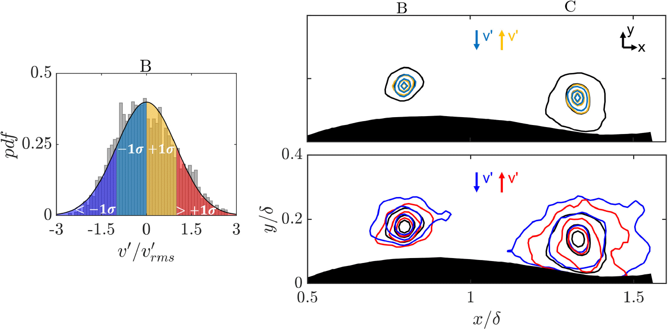
In order to further examine the anisotropy observed in the wall-normal velocity coherence around the cavity, $R_{v'v'}$
is conditioned based on the standard deviation of
$R_{v'v'}$
is conditioned based on the standard deviation of $v'$
(
$v'$
( $v'_{rms}$
) and the sign of
$v'_{rms}$
) and the sign of $v'$
(
$v'$
( $v'\gt 0$
:
$v'\gt 0$
: $R|_{v'\lt v'_{rms}}$
and
$R|_{v'\lt v'_{rms}}$
and $R|_{v'\gt v'_{rms}}$
;
$R|_{v'\gt v'_{rms}}$
; $v'\lt 0$
:
$v'\lt 0$
: $R|_{v'\gt -v'_{rms}}$
and
$R|_{v'\gt -v'_{rms}}$
and $R|_{v'\lt -v'_{rms}}$
, see figure 10). The conditional correlations (coloured lines in figure 10) are compared with the unconditional
$R|_{v'\lt -v'_{rms}}$
, see figure 10). The conditional correlations (coloured lines in figure 10) are compared with the unconditional $R_{v'v'}$
(black lines in figure 9 and figure 10). The spatial coherence and anisotropy observed in the unconditional
$R_{v'v'}$
(black lines in figure 9 and figure 10). The spatial coherence and anisotropy observed in the unconditional $R_{v'v'}$
are clearly due to high intensity events. For fluctuations with intensities
$R_{v'v'}$
are clearly due to high intensity events. For fluctuations with intensities $\lt v'_{rms}$
(of either sign), spatial coherence is limited and more isotropic compared with the global behaviour, while those with intensities
$\lt v'_{rms}$
(of either sign), spatial coherence is limited and more isotropic compared with the global behaviour, while those with intensities $\gt v'_{rms}$
(of either sign), a significant elongation in
$\gt v'_{rms}$
(of either sign), a significant elongation in $x$
is observed, leading to the observed anisotropy in the unconditional correlations. At the leeward side of the cavity, this high intensity, anisotropic behaviour is also seen to be prominent for
$x$
is observed, leading to the observed anisotropy in the unconditional correlations. At the leeward side of the cavity, this high intensity, anisotropic behaviour is also seen to be prominent for $v'\lt 0$
, thus for structures moving towards the cavity interface (see table 3 for an estimate). These relatively large coherent structures (with
$v'\lt 0$
, thus for structures moving towards the cavity interface (see table 3 for an estimate). These relatively large coherent structures (with $v'\lt 0$
) near the trailing edge of the cavity (where the cavity is observed to breakup and shed), can play an important role in the cavity’s form and stability: regions of downwards moving liquid (directed towards the cavity) can lead to pinch-offs at the cavity’s trailing edge, promoting its breakup and resulting in a shortened length. Along with this mechanism, other factors like the presence of re-entrant jets and small-scale wave instabilities at the cavity interface proposed in the literature (see for example Mäkiharju et al. (Reference Mäkiharju, Elbing, Wiggins, Schinasi, Vanden-Broeck, Perlin, Dowling and Ceccio2013); Zverkhovskyi (Reference Zverkhovskyi2014)) can shorten the cavity length. This shortening can have negative implications in ship air lubrication applications, where a minimal contact area between water and solid surface is sought, that is, achieving and maintaining the maximum possible cavity lengths. To establish the extent of such interactions, however, simultaneous time-resolved measurements of the instantaneous cavity shape and stability and TBL structuring would be required, which is out of the scope of the present study.
$v'\lt 0$
) near the trailing edge of the cavity (where the cavity is observed to breakup and shed), can play an important role in the cavity’s form and stability: regions of downwards moving liquid (directed towards the cavity) can lead to pinch-offs at the cavity’s trailing edge, promoting its breakup and resulting in a shortened length. Along with this mechanism, other factors like the presence of re-entrant jets and small-scale wave instabilities at the cavity interface proposed in the literature (see for example Mäkiharju et al. (Reference Mäkiharju, Elbing, Wiggins, Schinasi, Vanden-Broeck, Perlin, Dowling and Ceccio2013); Zverkhovskyi (Reference Zverkhovskyi2014)) can shorten the cavity length. This shortening can have negative implications in ship air lubrication applications, where a minimal contact area between water and solid surface is sought, that is, achieving and maintaining the maximum possible cavity lengths. To establish the extent of such interactions, however, simultaneous time-resolved measurements of the instantaneous cavity shape and stability and TBL structuring would be required, which is out of the scope of the present study.
Length scale ( $L_x$
and
$L_x$
and $L_y$
) estimates of conditioned
$L_y$
) estimates of conditioned $R_{v'v'}$
:
$R_{v'v'}$
: $R|_{v'\gt v'_{rms}}$
(red) and
$R|_{v'\gt v'_{rms}}$
(red) and $R|_{v'\lt -v'_{rms}}$
) (dark blue) contours in figure 10 (right panel bottom) measured at
$R|_{v'\lt -v'_{rms}}$
) (dark blue) contours in figure 10 (right panel bottom) measured at $0.4$
correlation level using an elliptical fit (see figure 9).
$0.4$
correlation level using an elliptical fit (see figure 9). $L_x$
and
$L_x$
and $L_y$
are lengths along the streamwise and wall-normal directions respectively
$L_y$
are lengths along the streamwise and wall-normal directions respectively
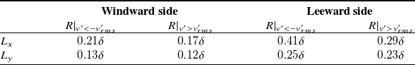
4. Conclusions
The TBL development over an air cavity was experimentally investigated using planar PIV. These type of flows are typically encountered in the application of ship air lubrication where the air cavity dynamics and morphology depend on the incoming flow conditions and vice versa. The present study provides for the first time an experimental insight into a subset of such flows: the response and development of a TBL to an air cavity formed at a specific incoming flow condition and air flow rate. The flow over the air cavity shares similarities to flow over solid bumps in the literature (Baskaran et al. Reference Baskaran, Smits and Joubert1987; Webster et al. Reference Webster, DeGraff and Eaton1996). However, unlike solid bumps, which have a fixed maximum thickness and length, the air cavity has a relatively variable geometry inherent to its dynamic nature. In addition, the presence of multiple pressure gradients and curvatures including a free-slip boundary, makes the behaviour of the TBL significantly more complex. Given the important role played by the geometry of solid bumps in the development of the incoming flow observed previously in the literature, the instantaneous geometries of the cavity were identified using a detection technique based on the thresholding of correlation values. The detection revealed a well-defined, asymmetric bump-like geometry at the spanwise-uniform region of the cavity also supported by visual observations. Statistics of the cavity geometry revealed the r.m.s. deviation of the maximum thickness and chord length of the cavity to be approximately $5.8\;\mathrm{\%}$
and
$5.8\;\mathrm{\%}$
and $5.2\;\mathrm{\%}$
, respectively, from the mean cavity shape, indicating that there were no significant deviations of the cavity from a bump-like geometry. The ratio of the incoming boundary layer thickness to the maximum thickness of the cavity was found to be approximately
$5.2\;\mathrm{\%}$
, respectively, from the mean cavity shape, indicating that there were no significant deviations of the cavity from a bump-like geometry. The ratio of the incoming boundary layer thickness to the maximum thickness of the cavity was found to be approximately $\delta /t_{max} = 12$
, which is considerably higher than ratios encountered in the solid bump studies of Baskaran et al. (Reference Baskaran, Smits and Joubert1987) and Webster et al. (Reference Webster, DeGraff and Eaton1996) (
$\delta /t_{max} = 12$
, which is considerably higher than ratios encountered in the solid bump studies of Baskaran et al. (Reference Baskaran, Smits and Joubert1987) and Webster et al. (Reference Webster, DeGraff and Eaton1996) ( $\delta /h = 0.25$
and
$\delta /h = 0.25$
and $\delta /h = 1.5$
, respectively,
$\delta /h = 1.5$
, respectively, $h$
being the height of the bump). Consequently, the TBL did not undergo separation at the leeward side of the cavity.
$h$
being the height of the bump). Consequently, the TBL did not undergo separation at the leeward side of the cavity.
The boundary layer thickness ( $\delta$
) and the mean streamwise velocity profiles were found to follow the trend set by alternating streamwise pressure gradients, consistent with previous works on flow over solid bumps: from an APG around the cavity leading edge, followed by a FPG over the windward side of the cavity and finally an APG over the leeward side of the cavity. Trends set by turbulence stresses (normalised in outer scales) particularly,
$\delta$
) and the mean streamwise velocity profiles were found to follow the trend set by alternating streamwise pressure gradients, consistent with previous works on flow over solid bumps: from an APG around the cavity leading edge, followed by a FPG over the windward side of the cavity and finally an APG over the leeward side of the cavity. Trends set by turbulence stresses (normalised in outer scales) particularly, $\overline {u'u'}$
and
$\overline {u'u'}$
and $-\overline {u'v'}$
, exhibited expected behaviours set by alternating streamwise pressure gradients: a weakening of stresses in the FPG region and an amplification of stresses in the APG region, mostly occurring in the lower part of the outer layer. The behaviour of
$-\overline {u'v'}$
, exhibited expected behaviours set by alternating streamwise pressure gradients: a weakening of stresses in the FPG region and an amplification of stresses in the APG region, mostly occurring in the lower part of the outer layer. The behaviour of $\overline {v'v'}$
, however, appeared to be largely different in character over the cavity: it was observed to amplify below
$\overline {v'v'}$
, however, appeared to be largely different in character over the cavity: it was observed to amplify below $y\approx 0.3\delta$
throughout the length of the cavity, even in the region where an attenuation of stress was expected due to a FPG. The amplification of
$y\approx 0.3\delta$
throughout the length of the cavity, even in the region where an attenuation of stress was expected due to a FPG. The amplification of $\overline {v'v'}$
was attributed to the dominance of the vertical momentum introduced by the air injection over any pressure gradient effects, particularly over the windward side of the cavity. Streamline curvature on the other hand, was concluded to be marginal, based on previous observations. The recovery of the TBL to its state upstream of the cavity is rapid, occurring within a boundary layer thickness, the latter still within the shedding region. However, effects of the APG imposed by the leading edge of the cavity remain present in the TBL in comparison with its baseline state (no cavity).
$\overline {v'v'}$
was attributed to the dominance of the vertical momentum introduced by the air injection over any pressure gradient effects, particularly over the windward side of the cavity. Streamline curvature on the other hand, was concluded to be marginal, based on previous observations. The recovery of the TBL to its state upstream of the cavity is rapid, occurring within a boundary layer thickness, the latter still within the shedding region. However, effects of the APG imposed by the leading edge of the cavity remain present in the TBL in comparison with its baseline state (no cavity).
Two-point correlations of the wall-normal velocity fluctuations ( $R_{v'v'}$
) at
$R_{v'v'}$
) at $y_{ref}=0.4\delta$
exhibited similar extent of coherence at all streamwise regions over the cavity, with no significant changes from the baseline case (no cavity). A local anisotropy and changes to the orientation of
$y_{ref}=0.4\delta$
exhibited similar extent of coherence at all streamwise regions over the cavity, with no significant changes from the baseline case (no cavity). A local anisotropy and changes to the orientation of $R_{v'v'}$
(following approximately the inclinations of the cavity) were observed at
$R_{v'v'}$
(following approximately the inclinations of the cavity) were observed at $y_{ref}=0.1\delta$
although more pronounced at the leeward side: the aspect ratio nearly doubled and the length reached the order of half the cavity length. The increased coherent extent of
$y_{ref}=0.1\delta$
although more pronounced at the leeward side: the aspect ratio nearly doubled and the length reached the order of half the cavity length. The increased coherent extent of $R_{v'v'}$
in a region subjected to an APG, in contrast to studies where a TBL was subjected to an APG alone, was attributed to the cumulative effect of multiple streamwise pressure gradients, resulting from a relatively slow response of the TBL to the local conditions of the cavity interface. The anisotropy in
$R_{v'v'}$
in a region subjected to an APG, in contrast to studies where a TBL was subjected to an APG alone, was attributed to the cumulative effect of multiple streamwise pressure gradients, resulting from a relatively slow response of the TBL to the local conditions of the cavity interface. The anisotropy in $R_{v'v'}$
due to the increased spatial coherence in
$R_{v'v'}$
due to the increased spatial coherence in $x$
was further shown to be a result of high amplitude events (
$x$
was further shown to be a result of high amplitude events ( $v'\gt v'_{rms}$
) and more pronounced for
$v'\gt v'_{rms}$
) and more pronounced for $v'\lt 0$
(moving towards the cavity) , especially at the leeward side. These relatively large coherent regions of liquid directed towards the cavity can play an important role in the formation of the latter, an aspect that is crucial in the application of ship air lubrication.
$v'\lt 0$
(moving towards the cavity) , especially at the leeward side. These relatively large coherent regions of liquid directed towards the cavity can play an important role in the formation of the latter, an aspect that is crucial in the application of ship air lubrication.
To sum up, the present study provides an insight into the physics of one aspect of the liquid–gas two-way coupling, namely, the response and development of a TBL in the presence of the air cavity; the complexity and lack of relevant studies on the topic highlight the need for future work. Further rigorous investigations with time-resolved measurements of the instantaneous cavity shape and the surrounding velocity field are necessary to study their interaction and isolate the different ingredients at play, such as alternating pressure gradients, surface curvature and the effects of air injection and a free-slip boundary condition, the latter aspects setting this family of flows apart from solid bump flows. Results and conclusions from this study are expected to not only provide insights regarding cavity formation, but also establish a baseline reference for geometries involving flow over gaseous layers while serving as a testbed for future studies examining variable inflow conditions and external perturbations.
Supplementary movies
Supplementary movies are available at https://doi.org/10.1017/flo.2025.10016.
Acknowledgements
The authors would like to gratefully acknowledge the help of E. Overmars and J. Ruijgrok in setting up the experiments at the Laboratory of Aero and Hydrodynamics at TU Delft. The authors would also like to thank the anonymous referees whose comments and suggestions helped improve the manuscript.
Data availability
Data will be made available on reasonable request.
Author contributions
Abhirath Anand: Investigation (lead), Conceptualisation, Methodology, Visualisation, Validation, Formal analysis, Writing – original draft. Lina Nikolaidou: Investigation (support), Conceptualisation, Methodology, Writing – review & editing. Christian Poelma: Conceptualisation, Methodology, Supervision, Writing – review & editing. Angeliki Laskari: Conceptualisation, Methodology, Supervision, Writing – review & editing.
Funding
This research received no specific grant from any funding agency, commercial or not-for-profit sectors.
Competing interests
The authors declare no conflict of interest.
Ethical standards
The research meets all ethical guidelines, including adherence to the legal requirements of the study country.
Appendix: potential relationship between instantaneous cavity shape and mean liquid velocity
We attempt to quantify the effects of the instantaneous cavity deviations on the mean velocity of the surrounding liquid flow. To this end, we conditionally average the TBL profiles on the extreme excursions (with respect to the mean) of the cavity interface. The instantaneous cavity shapes are divided into three regions (see figure 11) corresponding to the three streamwise locations considered over the cavity ( $x'_3 = 0.15$
,
$x'_3 = 0.15$
, $x'_4 = 0.47$
and
$x'_4 = 0.47$
and $x'_5 = 0.77$
, see for example figure 5).
$x'_5 = 0.77$
, see for example figure 5).
Mean cavity interface (solid blue line) with representative examples of instantaneous cavity interface polynomial fits (solid black lines; see inset of figure 3 bottom for instantaneous cavity interface detected). Shaded areas represent the three regions considered in the conditional analysis shown in figure 12.
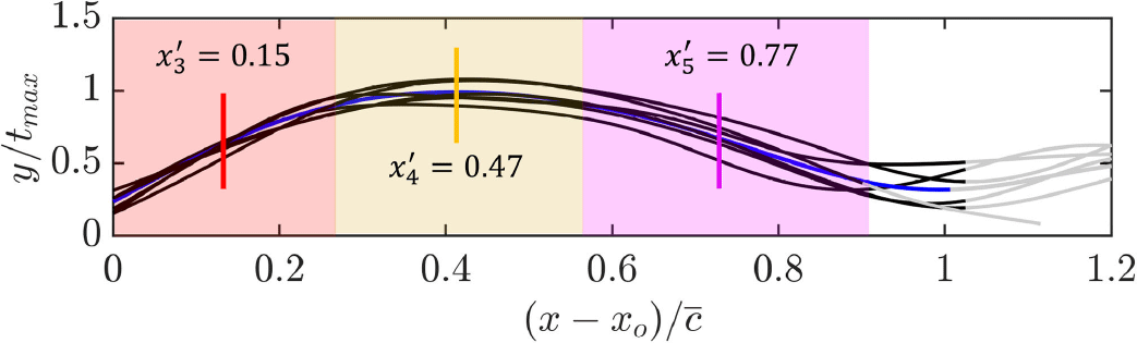
Conditional mean streamwise velocity profiles on the instantaneous interface location (spatial average of regions shown in figure 11) being above (red dashed line) and below (blue dashed line) one standard deviation ( $\sigma$
) from the mean cavity interface. Also shown is the unconditional mean streamwise velocity profile (continuous lines with symbols) which is computed over the mean cavity interface. Flow is from left to right.
$\sigma$
) from the mean cavity interface. Also shown is the unconditional mean streamwise velocity profile (continuous lines with symbols) which is computed over the mean cavity interface. Flow is from left to right.
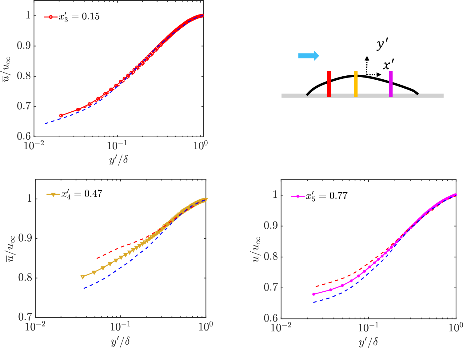
The instantaneous interface location is spatially averaged within these regions to obtain a representative value. The mean velocity is then conditioned on these representative interface locations being above (red dashed line in figure 12) or below (blue dashed line in figure 12) $1\sigma$
from the mean. The conditional profiles are compared with the unconditional mean streamwise velocity profile that is computed over the mean cavity interface. The mean velocity of the surrounding liquid is observed to increase (decrease) when the instantaneous interface is above (below) the mean, more prominently observed at
$1\sigma$
from the mean. The conditional profiles are compared with the unconditional mean streamwise velocity profile that is computed over the mean cavity interface. The mean velocity of the surrounding liquid is observed to increase (decrease) when the instantaneous interface is above (below) the mean, more prominently observed at $x'_{4}$
and
$x'_{4}$
and $x'_{5}$
. To provide further insight into the influence of the instantaneous shapes of the cavity on the higher-order statistics of the flow such as turbulent stresses, however, would require time-resolved data. Since turbulent stresses require a relatively longer time to adjust to the surrounding conditions (for example to the instantaneous shape of the cavity) in comparison with the mean flow, history effects are expected to be important making the requirement of time-resolved data all the more necessary.
$x'_{5}$
. To provide further insight into the influence of the instantaneous shapes of the cavity on the higher-order statistics of the flow such as turbulent stresses, however, would require time-resolved data. Since turbulent stresses require a relatively longer time to adjust to the surrounding conditions (for example to the instantaneous shape of the cavity) in comparison with the mean flow, history effects are expected to be important making the requirement of time-resolved data all the more necessary.


 Open access