


Impact Statement
We present a velocimetry method that infers time-dependent flow speeds using visual observations of flow–structure interactions such as the swaying of trees. This can alleviate the need to directly instrument or visualize the flow to quantify its speed, instead relying on pre-existing objects in an environment that are deflecting due to the incident flow. The method has the potential to turn ubiquitous objects like trees into abundant, natural, environmental flow sensors for applications such as weather forecasting, wind energy resource quantification and studies of wildfire propagation.
1. Introduction
Fluid–structure interactions such as the bending and swaying of trees in the wind provide visual cues that contain information about the surrounding flow. If visual measurements of deflections can be used to infer quantitative estimates of local wind speeds, then common objects like trees could be used as abundant natural anemometers, requiring only non-intrusive visual access to record wind speed measurements. This would potentially be useful in applications such as data assimilation for weather forecasting, wind energy resource quantification and understanding wildfire behaviour. Recent work has examined this visual anemometry task through a data-driven approach, where a neural-network-based model was trained to output wind speeds based on input videos of flags and trees in naturally occurring wind (Reference Cardona, Howland and DabiriCardona et al., 2019). However, achieving a data-driven model that would generalize to a wide variety of objects (e.g. trees of different sizes and species) could potentially require an extensive data collection campaign. Physical models for fluid–structure interactions may be advantageous in providing a framework that could be used for visual anemometry across a broader range of structures. Here, we focus on objects that can be modelled as cantilever beams under wind loading.
Flow-sensing cantilevers are found in nature. For instance, the lateral line system allows fish to sense the surrounding flow via the deflection of hair-like structures (Reference Bleckmann and ZelickBleckmann & Zelick, 2009). Artificial lateral line sensors have been developed to mimic this flow-sensing function as discussed by Reference ShizheShizhe (Reference Shizhe2014). Cantilever beam deflections have also been used to measure wind speeds specifically. Reference TrittonTritton (Reference Tritton1959) used optical measurements of cantilevered quartz fibre deflections, and Reference Krautse and FralickKrautse & Fralick (Reference Krautse and Fralick1977) used strain gauge measurements of millimetre-scale silicone beams. These drag-based anemometers relied on knowledge of the material properties of the beam. These physical properties could then be used in conjunction with beam bending theory to calculate the drag force on the beam and quantify the wind speed. In these cases, the beam materials were specifically chosen for sensing purposes. Another example of cantilever deflection-based anemometry can be seen in Reference Barth, Koch, Kittel, Peinke, Burgold and WurmusBarth et al. (Reference Barth, Koch, Kittel, Peinke, Burgold and Wurmus2005), where the deflection of a millimetre-scale cantilever affects the position of a reflected laser, which is calibrated to measure flow speeds.
While these prior studies have shown success in measuring flow speeds by instrumenting the flow with cantilevers specifically designed and intended for sensing, the present work aims to extend the concept of flow-sensing cantilevers so that it can ultimately be used with a variety of pre-existing structures in an environment without further instrumenting the flow. Natural structures such as trees have material properties that are unknown a priori, and they are more geometrically complex than single beams. Hence, in this work we exploit simplified models of the flow–structure interactions to avoid the need for direct consideration of these details, while still capturing the physical influence of the wind on structure deformation. By this approach, we can leverage the prevalence of trees and other vegetation in both rural and built environments for use in visual anemometry.
Approximate wind speed scales have been developed based on field observations of fluid–structure interactions in the past. The Fujita scale, for example, is used to infer tornado wind speed based on the damage to structures in its path (Reference Doswell, Brooks and DotzekDoswell et al., 2009). This has been particularly useful since more conventional wind speed measurements are rare and difficult to obtain for tornadoes. The Beaufort scale is another well-known wind speed scale that relies on visual cues. The version of the scale adapted for use on land employs qualitative descriptions of tree behaviour (e.g. branch motion or breaking of twigs) to estimate an instantaneous wind speed range, and it has also been applied to region-specific vegetation (Reference JemisonJemison, 1934). Visual observations of trees and other vegetation have also been used to estimate mean annual wind speeds. The Griggs–Putnam index uses qualitative descriptions of tree deformation to categorize mean annual wind speeds into seven binned increments of 1–2 ms $^{-1}$ (Reference Wade and HewsonWade & Hewson, 1979). Time series measurements of tree deformations and a physical model for the fluid–structure interactions may allow for an extension to quantitative, instantaneous flow speed measurements.
Wind–tree interactions have been widely studied (Reference de Langrede Langre, 2008). Prior investigations have used various forms of cantilever beam models to describe tree behaviour. For instance, Reference KemperKemper (Reference Kemper1968), Reference Morgan and CannellMorgan & Cannell (Reference Morgan and Cannell1987) and Reference GardinerGardiner (Reference Gardiner1992) compared tree deflections to tapered cantilever beams. The relationship between wind speed and drag force on trees has also been explored, in particular with regard to the drag reduction that results from large deformations of the tree crown. Several studies have observed and quantified the drag on trees as a function of wind speed (Reference FraserFraser, 1962; Reference Kane and SmileyKane & Smiley, 2006; Reference Koizumi, Motoyama, Sawata, Sasaki and HiraiKoizumi et al., 2010; Reference de Langre, Gutierrez and Cosséde Langre et al., 2012; Reference Manickathan, Defraeye, Allegrini, Derome and CarmelietManickathan et al., 2018; Reference MayheadMayhead, 1973; Reference Rudnicki, Mitchell and NovakRudnicki et al., 2004; Reference Vollsinger, Mitchell, Byrne, Novak and RudnickiVollsinger et al., 2005). Despite the complexities of wind–tree interactions, this prior work suggests that the structural behaviour under wind loading can be generalized in physical models.
The present work aims to infer incident wind speed measurements from observations of cantilevered cylinders and trees. We achieve this visual anemometry without a priori knowledge of the material properties of the structures, as is the case for application to natural vegetation. A model for the relationship between the drag force and mean deflection is proposed. Using this model, normalized wind speeds can be approximated based only on the measured deflections of a structure, where the normalization is based on the measured wind speed and deformation at a selected reference time. The model was tested and compared to ground truth anemometer-measured wind speeds for both cantilevered cylinders and trees in wind tunnel experiments. Given that object deflections can be observed from videos, this method can serve as a non-intrusive technique to measure normalized wind speeds, where dimensional velocities may be recovered with a single calibration measurement at a reference wind speed. This eliminates the need to directly instrument or visualize the flow for quantitative characterization.
2. Physical Model
A physical model was used to relate wind speed to deflections based on a force balance. The dynamic pressure,  $p$, on an object in flow is proportional to the product of the fluid density, $\rho$, and the square of the mean incident wind speed, $U$ (Reference BatchelorBatchelor, 2000). The mean force of the wind, $F_W$, is given by multiplying $p$ by the projected frontal area, $A$, and is therefore proportional to $\rho U^2A$:
 \begin{equation} F_W = pA \propto \rho U^2 A. \end{equation}
We model the deflection of the structure following Hooke's law
 \begin{equation} F_E = \kappa\delta, \end{equation}
where  $F_E$ is the elastic restoring force, $\kappa$ is the elastic constant and $\delta$ is the deflection of the free end of the cantilever. This model is applicable for small deflections under point loads or distributed loads, with differences in the configuration of loading captured in the form of the constant of proportionality. For a cantilever of constant cross-section subject to a uniformly distributed load, the relationship between force per unit length, $f$, and the tip deflection given by Euler–Bernoulli beam theory follows
 \begin{equation} f = \left( \frac{8EI}{L^4} \right)\delta, \end{equation}
where  $E$ is the Young's modulus of the material, $I$ is the area moment of inertia and $L$ is the length of the beam. In this case, the elastic constant is related to the geometric and material properties of the cantilever. The total force on the beam is equal to $fL$, and the elastic constant as defined in (2) is $\kappa = {8EI}/{L^3}$.
A balance of the forces in (1) and (2) above gives a relationship between the incident flow speed and the structure deformation
 \begin{equation} U \propto \sqrt{\frac{\kappa\delta}{\rho A}}. \end{equation}
Furthermore, assuming that  $\rho$, $\kappa$ and $A$ remain constant under the conditions of interest, the wind speed normalized by a non-zero reference condition characterized by $U_0$ and $\delta _0$ is given by
 \begin{equation} \frac{U}{U_0} = \sqrt{\frac{\delta}{\delta_0}}. \end{equation}
The normalized wind speed given in (5) is independent of the material properties of the structure, and the dimensional wind speed can be recovered given only a measurement of  $\delta$ and the reference condition ( $U_0$, $\delta _0$). In the measurements described below, we examine the regime of validity of the model in (5).
2.1. Modification for Tree Crown Deformation
Experimental observations by Reference Roodbaraky, Baker, Dawson and WrightRoodbaraky et al. (Reference Roodbaraky, Baker, Dawson and Wright1994) have shown that load–deflection curves for various tree species appear to be linear, which suggests that the linear relationship proposed in (2) is appropriate to use for trees. However, (5) assumes that the frontal area of the structure is constant for all incident wind conditions. Prior observations have shown a reduced growth in drag force on trees with increasing  $U$ (Reference FraserFraser, 1962; Reference Kane and SmileyKane & Smiley, 2006; Reference Koizumi, Motoyama, Sawata, Sasaki and HiraiKoizumi et al., 2010; Reference de Langre, Gutierrez and Cosséde Langre et al., 2012; Reference Manickathan, Defraeye, Allegrini, Derome and CarmelietManickathan et al., 2018; Reference MayheadMayhead, 1973). The drag reduction is attributed to reconfiguration of the tree crown which leads to streamlining as a result of the change in area (Reference Harder, Speck, Hurd and SpeckHarder et al., 2004; Reference Rudnicki, Mitchell and NovakRudnicki et al., 2004; Reference Vollsinger, Mitchell, Byrne, Novak and RudnickiVollsinger et al., 2005; Reference Manickathan, Defraeye, Allegrini, Derome and CarmelietManickathan et al., 2018). The effect of the changing area has often been taken into account through the use of a Vogel number (Reference VogelVogel, 1989), $\beta$, and the drag is assumed to grow as $U^{2 + \beta }$, where $\beta$ has a negative value to compensate for the streamlining effect. The Vogel number has been found to vary between tree species, with typical magnitudes in the range of $\mathcal {O}([0.1, 1])$ (Reference de Langre, Gutierrez and Cosséde Langre et al., 2012; Reference Manickathan, Defraeye, Allegrini, Derome and CarmelietManickathan et al., 2018). In general, the value of $\beta$ may be unknown for a tree of interest without extensive testing. Therefore, instead of accounting for reconfiguration by using a Vogel exponent, the changing instantaneous frontal area was taken directly into account. Considering that $A$ changes with wind speed, the normalized wind speed becomes
 \begin{equation} \frac{U}{U_0} = \sqrt{\frac{\delta A_0}{\delta_0 A}}, \end{equation}
where  $A_0$ is the frontal area of the tree at reference speed $U_0$. Where a projection of the frontal area of the structure is not available, the change in area can be approximated by assuming $A \propto h^2$, where $h$ is the projected tree height. This gives the modified form of the model to determine normalized wind speeds from tree deflections
 \begin{equation} \frac{U}{U_0} = \sqrt{\frac{\delta h_0^2}{\delta_0 h^2}}. \end{equation}
3. Experimental Methods
3.1. Cantilevered Cylinder Deformation Measurements
A first set of experiments studied deflections of flexible cylinders with circular cross-section. These canonical structures contrast with more complex tree geometries studied subsequently. Experiments were carried out in a  $2.06\ \textrm {m} \times 1.97\ \textrm {m}$ cross-section open-circuit wind tunnel (more details can be found in Reference Brownstein, Wei and DabiriBrownstein et al., 2019). Mean flow speeds were measured using a factory-calibrated anemometer (Dwyer Series 641RM Air Velocity Transmitter) with a digital readout. The anemometer was accurate to $3\,\%$ of full scale, where full scale was set to 15 ms $^{-1}$. Each test cylinder was rigidly mounted to the ceiling of the tunnel, and subjected to three mean flow speeds ( $U=[4.5, 5.6, 6.6] \pm 0.5$ ms $^{-1}$). The maximum blockage ratio in the wind tunnel based on the projected area of the test cylinder and mounting apparatus was $4.0\,\%$. A schematic of the set-up is shown in Figure 1.
Schematic of experimental set-up to measure cylinder deflection showing (a) side and (b) rear views. Directions of flow and gravity are indicated. Cylinder dimensions are to scale for the polyvinyl chloride (PVC) tube of  $D= \textit{5.1} \pm \textit{0.1}$ cm, $L = \textit{1.52} \pm \textit{0.01}$ m (the cylinder with the largest frontal area).

The deflection for a given cylinder and wind speed was measured by tracking the free end of the cylinder in video frames collected at 240 frames per second (f.p.s.) with a resolution of  $720 \times 1280$ pixels. The recording began with the cylinder at rest. The wind tunnel was then turned on and allowed to reach a steady-state speed. Measurements were collected for 60 s at each steady-state speed. The centre of the cylinder surface was detected in each frame using a two-stage Hough transform (Reference Yuen, Princen, Dlingworth and KittlerYuen et al., 1990) in the MATLAB Image Processing Toolbox. The tip deflection, $\delta$, was determined by calculating the streamwise displacement of the centre for each frame in the 60 s steady-state period with respect to its position under no wind load (Figure 2). Examples of streamwise displacement versus time are shown in Figure 3. Mean displacements were typically on the order of 250 pixels, corresponding to physical dimensions of approximately 10 cm. The normalized wind speed, $U/U_0$ was calculated by taking the mean of (5). Note that while the cylinders were also free to move in the spanwise direction, spanwise displacements were an order of magnitude smaller than streamwise displacements and had a negligible mean value. Examples of cylinder free end trajectories showing both streamwise and spanwise displacements can be seen in the supplementary material, Figure S1 available at https://doi.org/10.1017/flo.2021.3.
Representative frames showing the displacement of the cylinder free end (PVC tube,  $D = \textit{5.1} \pm \textit{0.1}$ cm). Top: cylinder surface under no wind load. Bottom: displaced cylinder subject to incident flow speed $U = \textit{5.6} \pm \textit{0.5}$ ms $^{-1}$, with streamwise displacement, $\delta$, shown in reference to centre position under no load. Cylinder centres indicated with ‘ $+$’.
$+$’.

Examples of free end streamwise displacement vs. time over the 60 s steady-state periods for a PVC cylinder ( $D = \textit{3.8} \pm \textit{0.1}$ cm) for $U= [\textit{4.5}, \textit{5.6}, \textit{6.6}] \pm \textit{0.5}$ ms $^{-1}$ (lines shaded from light to dark with increasing $U$). Mean displacements are indicated with dashed lines. The observed streamwise oscillations are consistent with previous studies in steady flow (Reference KingKing, 1974).

Six unique cylinders were tested. Cylinder aspect ratios ( $L/D$) ranged from 30 to 48, and Reynolds numbers (Re D) based on cylinder diameters ranged from $1.0 \times 10^4$ to $2.2\times 10^4$. For rigid cylinders in this range of $Re_D$, the drag coefficient, $C_D$, should remain relatively constant, especially since the sharp drop in $C_D$ for cylinders is typically observed to occur at higher $Re_D$ ( $\mathcal {O}(10^5)$) (Reference RoshkoRoshko, 1961). Four of the cylinders were cut from lengths of soft, flexible PVC tubing (Masterkleer, Durometer 65A) with wall thickness $t= 0.6 \pm 0.1$ cm, length $L= 1.52 \pm 0.01$ m, and outer diameters $D \in [3.2, 5.1] \pm 0.1$ cm. The unprocessed PVC tubing tended to have some amount of curvature under no load. To achieve right cylindrical specimens, the PVC tubing was heated with boiling water and allowed to cool in a straightened position. To ensure that the effect of any remaining curvature leading to imperfect cylindrical shape did not systematically bias results, each PVC tube was tested three times, and rotated by $90^\circ$ about its axis in the mounting clamp in each subsequent test.
Two other cylinders of different types were tested in addition to the PVC tubes for the purpose of validating model applicability on cylinders with varying characteristics. One was a solid polyurethane rubber rod (medium soft, Durometer 40A) with dimensions  $L = 1.22 \pm 0.01$ m and $D = 3.2 \pm 0.1$ cm. The final specimen was a hollow acrylonitrile butadiene styrene (ABS) tube ( $L = 1.55 \pm 0.01$ m, $D = 3.2 \pm 0.1$ cm, $t = 0.3 \pm 0.1$ cm) with a steel compression spring at its base (spring rate of 2.8 N mm $^{-1}$) held by the mounting clamp at the tunnel roof. In this case, the ABS cylinder acted as a rigid body rather than a flexible cylinder like the other specimens, and the deflection was facilitated primarily by bending of the spring at its base. Table 1 summarizes the properties of the six cylinders tested.
Summary of test cylinder properties including the material, outer diameter,  $D$, wall thickness of hollow tubes, $t$, length, $L$, aspect ratio, $L/D$, and Young's modulus, $E$.
$E$.

aNote that, for the PVC and polyurethane rubber cylinders, exact values of Young's modulus were not known, and were therefore approximated based on the reported Shore hardness values using the relationship given in Gent (Reference Gent1958).
3.2. Tree Deformation Measurements
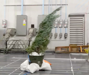
Measurements of two natural trees were conducted in a second, larger open-circuit wind tunnel of cross-section  $2.88\ \textrm {m} \times 2.88\ \textrm {m}$. Deflections were measured for the two potted trees: a conifer commonly known as a juniper tree (Juniperus scopulorum), and a broad-leaved bay laurel tree (Laurus nobilis). Approximate tree dimensions are given in Table 2. Trees were positioned using sand bags to weight down the pots and keep them in place. The tunnel was run in a uniform flow configuration at four distinct mean flow speeds spanning the tunnel range ( $U = [3.3, 6.0, 8.8, 11.4] \pm 0.5$ ms $^{-1}$), which were measured using the factory-calibrated anemometer (Dwyer Series 641RM Air Velocity Transmitter). Reynolds numbers based on a length scale of $A^{1/2}$, where $A$ is the approximate frontal area of the tree under no load, ranged from $1.7 \times 10^5$ to $6.3 \times 10^5$. The maximum blockage ratio based on projected frontal area was 8.4 $\,\%$.
Tree properties including tree height,  $L$, measured from base to tip, frontal area, $A$, and trunk diameter at breast height, $DBH$. Approximate heights and areas were measured using photos taken from downstream of the trees under no wind load. Note values of $A$ were estimated using the outer envelope of the trees, and do not incorporate leaf density.

The camera was angled perpendicular to the flow direction to capture video of the streamwise tree deflections for 110 s at each steady-state flow speed. Videos were recorded at 240 f.p.s. with a resolution of  $720 \times 1280$ pixels. A random sample of frames was chosen to measure the tip deflections. For each 10 s clip of video data, 10 frames were randomly selected. This yielded 110 sample frames for each flow speed. Values for $\delta$ and $h$ were measured over the 110 samples. The pixel position of highest point on the tree was manually identified in each sample frame using MATLAB. This position was used to calculate $h$ and $\delta$ for each frame. The streamwise position of the highest point on the tree under no wind load marked $\delta = 0$, and $h$ was measured in reference to the base of the tree. Representative measurements of $h$ and $\delta$ are shown in Figure 4. The values of $h$ and $\delta$ found for each frame were used to calculate $U/U_0$ as shown in (7). The mean value of was taken over the 110 sample frames for each flow speed.
Example measurements of streamwise deflection,  $\delta$, and projected height, $h$, for the juniper tree (a,b) and the laurel tree (c,d). Measurements were made in reference to treetop position under no wind load (a,c). Resulting measurements of tree deformation for $U= \textit{11.4}$ ms $^{-1}$ are shown in (b,d).

4. Results
4.1. Normalized Wind Speeds from Cylinder Deflections
Normalized wind speeds inferred from visual measurements and (5) are compared to ground truth anemometer-measured values in Figure 5. Results are shown for all six test cylinders. Each datapoint represents  $U/U_0$ calculated using (5) for a particular test cylinder based on deflections $\delta$ and $\delta _0$ at wind speeds $U$ and $U_0$ respectively. As discussed in § 3.1, one reference condition ( $U_0$, $\delta _0$) must be known to calculate $U/U_0$. The results shown in Figure 5 include datapoints calculated using each of the three distinct mean flow speeds ( $U= [4.5, 5.6, 6.6] \pm 0.5$ ms $^{-1}$) as the reference, $U_0$, to determine $U/U_0$ for the other two tunnel speeds. Thus, using each combination of two wind speeds to obtain $U/U_0$ yields six ground truth values for which visually measured results can be compared (two datapoints for each distinct reference wind speed). Distinct markers are used to denote datapoints calculated with each particular value of $U_0$. Representative error bars are shown for the cylinder with the largest overall error values (the polyurethane rubber cylinder). The error bars were of the same order of magnitude for all cylinders. Horizontal error bars were calculated by propagating the uncertainty from anemometer accuracy through the ratio $U/U_0$. Vertical error bars were calculated based on the standard deviation of deflections over the tracking period, which were propagated through (5). The dashed black line shows the exact one-to-one relationship that would indicate perfect agreement between visually measured speeds and ground truth values. There is strong agreement between the visual and ground truth measurements.
Visually measured normalized wind speed vs. ground truth for all test cylinders. Marker colours indicate unique cylinders, and marker types indicate the reference speed,  $U_0$. The dashed black line represents unity.

4.2. Normalized Wind Speeds from Tree Deflections
Visually measured normalized wind speeds versus ground truth normalized wind speeds are plotted in Figure 6a for all test objects including the two trees and six cylinders. Note that cylinder datapoints are the same as they appear in Figure 5, but are also included in Figure 6a for ease of comparison between cylinder and tree results. The model accounting for changing frontal area, (7), was used to calculate the visually measured normalized wind speeds for the trees. Each of the four tunnel speeds used in the tree experiments ( $U = [3.3, 6.0, 8.8, 11.4] \pm 0.5$ ms $^{-1}$), was taken as a reference speed $U_0$ in combination with the other three distinct speeds for a total of 12 ground truth values. Once again, distinct markers have been used to show points calculated with each particular reference speed. The trees were subjected to a wider range of wind speeds than the cylinders based on tunnel capabilities, which led to results across a wider range of ground truth values ( $U/U_0 \in [0.3, 3.5]$ for the trees compared to $U/U_0 \in [0.7, 1.5]$ for the cylinders), as visible in Figure 6a. The per cent error of visual measurements compared to ground truth is shown in Figure 6b. Dimensional wind speeds recovered by multiplying the visually measured normalized speed by the reference speed, $U_0$, are shown in Figure 7. The accuracy of the visual measurement approach is validated in the comparison with ground truth. The visual measurements appear to agree well with ground truth measurements, but do modestly underestimate the ground truth at high wind speeds. This could be associated with the limitation in our estimate of area change, as we assumed $A \propto h^2$ to incorporate the tree crown deformation given only a side view of the tree. In addition, the breakdown of the model at large values of $U/U_0$ suggests a potential departure from the assumptions of the linear model utilized in computing the wind speed. We examine this latter possibility in more detail in the following section.
(a) Visually measured normalized wind speed vs. ground truth for trees and cylinders. Marker colours indicate the sample object, and marker types indicate the reference wind speed used in the visual measurements. The dashed black line represents unity indicating perfect model agreement. (b) Per cent error of visual measurement compared to ground truth.

(a) Visually measured dimensional wind speed vs. ground truth for trees and cylinders. Marker colours indicate the sample object, and marker types indicate the reference wind speed used in the visual measurements. The dashed black line represents unity indicating perfect model agreement. (b) Per cent error of the dimensional visual measurement compared to ground truth.

5. Discussion and Conclusions
Wind speed measurements inferred from structure kinematics showed strong agreement with the ground truth measurements for both the cylinders and the trees, as seen in Figures 5 and 6. This suggests that flow–structure interactions can be leveraged to infer local wind conditions without a priori knowledge of the material properties of the structure, and without visualizing or instrumenting the flow itself.
The agreement in normalized wind speed is particularly good at lower values of  $U/U_0$, but there is more discrepancy at higher values. As seen in Figure 6b, the per cent error in the visually measured normalized speed increases in magnitude as the ground truth normalized speed departs from a value of 1. One factor that may contribute the discrepancy is that the model assumptions (e.g. the linear assumption of Hooke's law) become less valid at higher wind speeds where there are larger forces acting on the structures causing larger deflections. For instance, assuming a linear relationship for a cantilever beam subject to a uniformly distributed load or a point load overestimates the tip deflection when deformations are large (Reference RohdeRohde, 1953; Reference Bisshopp and DruckerBisshopp & Drucker, 1945). This linear model would then underestimate the wind speed corresponding to a given deflection. This is reflected in the overestimates for ground truth values of $U/U_0<1$ and the underestimates for ground truth values of $U/U_0>1$ in Figure 6b. Figure 8 shows the deflections expected using nonlinear beam bending models for both a uniformly distributed load (Reference RohdeRohde, 1953) and a point load (Reference Bisshopp and DruckerBisshopp & Drucker, 1945).
Normalized deflection ( $\delta / L$) of a cantilever beam vs. normalized force ( ${FL^2}/{EI}$). Curves are given for nonlinear models for a uniformly distributed load and for a point load reproduced from Reference RohdeRohde (Reference Rohde1953) and Reference Bisshopp and DruckerBisshopp & Drucker (Reference Bisshopp and Drucker1945) respectively, shown along with the linear relationships given by elementary theory. The maximum deflection observed in the present work for the juniper tree, laurel tree and cylinders are shown with dashed black lines

For both loading conditions, the nonlinear bending models start to noticeably depart from the linear models at deflections greater than  $\delta / L \approx 0.2$. Although the deflections observed for the cylinders and the laurel tree typically fell within the linear regime, the maximum deflections observed for the juniper tree were large enough to expect a significant departure. Notably, the juniper tree also yielded the highest error in visual wind speed measurements of the objects tested, particularly for datapoints that relied on deflections at the highest wind speed of 11.4 ms $^{-1}$ (Figure 6b).
To further consider the effects of large deflections of the juniper tree, the nonlinear models discussed in Reference RohdeRohde (Reference Rohde1953) and Reference Bisshopp and DruckerBisshopp & Drucker (Reference Bisshopp and Drucker1945) were used to correct the visual wind speed measurements. Note that the nonlinear models incorporate additional assumptions regarding the loading configuration, i.e. a point load at the tip (Reference Bisshopp and DruckerBisshopp & Drucker, 1945) or a uniformly distributed load (Reference RohdeRohde, 1953). While neither of these models strictly captures the real tree loading, they provide a means to conceptually assess the effect of nonlinearity. Cubic spline interpolation was used to obtain numerical functions for the nonlinear bending models from the curves shown in Figure 8. Observed values of  $\delta / L$ for the juniper tree were used to determine the expected normalized force according to the nonlinear models. This was used to find the effective deflection, $\hat {\delta }$, that would have been expected using the linear models with the same given force. Finally, the values of $\hat {\delta }$ were used to obtain the normalized wind speed measurements from (7). The results of these corrections for large bending are shown in Figure 9. While the error in visual measurements is not eliminated, the maximum error is reduced. For the linear model, the magnitude of error generally increased as larger wind speeds were involved in the calculation and $U/U_0$ departed from a value of 1. This trend is no longer apparent after the corrections for large bending have been applied Figure 9b. This suggests that the nonlinearity not captured by the original model likely plays a role in the increased error at higher wind speeds. It is possible that the application of other beam bending models meant for large deformations may improve agreement. Prior works have successfully described the bending behaviour of sapling trunks using tapered cantilevered beams models for analysing large deflections (Reference KemperKemper, 1968; Reference Morgan and CannellMorgan & Cannell, 1987; Reference GardinerGardiner, 1992). However, these more complex models required knowledge the flexural rigidity and the taper of the trunk, both of which may be unknown.
(a) Visually measured normalized wind speed vs. ground truth for the juniper tree using original linear model as well as models corrected according to the nonlinear models for beam bending under a point load (Reference Bisshopp and DruckerBisshopp & Drucker, 1945) and distributed load (Reference RohdeRohde, 1953). (b) Per cent error of visual measurement compared to ground truth.

Future studies may consider the use of a second camera aligned with the direction of flow to capture the instantaneous frontal area of the trees. This would enable validation of the model assumption  $A \propto h^2$ applied in (7). However, in practice, for many potential field applications it is beneficial to use only a single camera, as this reduces the complexity of the set-up and does not require access to multiple spatial locations surrounding the object of interest.
In the present work, the flow incident on the structures is designed to be spatially uniform. However, wind speeds in the near-surface region of the atmospheric boundary layer can vary with height above the ground,  $z$. A common model is the log wind profile
 \begin{equation} U(z) = \frac{u^ * }{K}\ln \left( \frac{z + d}{z_0} \right), \end{equation}
where  $u^*$ is the friction velocity, $K$ is the von Kármán constant ( $K \approx 0.4$), $d$ is the displacement height and $z_0$ is the surface roughness (Reference StullStull, 1988). The model presented here is still applicable for the loading on a cantilever beam resulting from the wind profile in (8). Under linear beam theory, the equation for tip displacement, $\delta$, is a linear differential equation. Hence, the principle of superposition applies, and the deflection from an arbitrary distributed load can be determined by superposing the solutions for the differential load at each point along the length of the beam (Reference Bauchau and CraigBauchau & Craig, 2009). The tip deflection due to a point load, $P$, acting at a height of $z$ along the beam is given by
 \begin{equation} \delta = \frac{P z^2 (3L - z)}{6EI}. \end{equation}
Thus, for a distributed force per unit length,  $f(z)$, the resulting tip deflection can be calculated as
 \begin{equation} \delta = \frac{1}{6EI} \int_{0}^{L} f z^2 (3L - z)\,\textrm{d} z. \end{equation}
Since the force from the wind is proportional to the square of the wind speed ((1)), the distributed load due to the log wind profile is given by  $f(z) = c U^2(z)$, where $c$ is a constant, resulting in the tip deflection
 \begin{equation} \delta = \frac{c \left(\dfrac{u^ * }{K}\right)^2}{6EI} \int_{d}^{L} \ln^2 \left( \frac{z + d}{z_0} \right) z^2 (3L - z)\,\textrm{d}z. \end{equation}
If  $z_0$ and $d$ remain constant for the conditions of interest (i.e. the shape of the $U(z)$ remains the same), then it follows from (8) that $u^* \propto U(L)$. In this case, since $u^*$ is the only component of 5.4 that changes with the mean wind speed, the relationship $U(L) \propto \sqrt {\delta }$ applies, and thus, the formulation of the model given in (5) can still be used to calculate the normalized wind speeds. In general, this approach of calculating $\delta$ from linear beam theory with a distributed load resulting from a particular wind profile will show that (5) is applicable if the shape of $U(z)$ remains the same between the reference and desired measurement conditions, with its magnitude scaling with the mean wind speed at the height of interest. This does not take into account the tree crown deformation, which may also vary with $z$. Future studies may consider this effect, as well as the influence of diurnal and seasonal variation of the velocity profile in the atmospheric boundary layer.
A further limitation of the present work is the need for a calibration reference ( $U_0$, $\delta _0$) to convert the normalized wind speeds to dimensional quantities. While the dimensional wind speeds are needed to determine other dimensional quantities such as kinetic energy flux, the normalized measurements may be sufficient for determining other useful flow characteristics even without calibration. For example, the shape factor, $k$, of the probability density function of a Weibull distribution of wind speeds can be determined using the normalized wind speed measurements. Weibull distributions are often used to characterize wind speed data (Reference Takle and BrownTakle & Brown, 1977) and are useful for applications such as assessing sites for wind energy generation (Reference Justus, Hargraves and YalcinJustus et al., 1976). The maximum likelihood method is commonly used to determine the Weibull distribution parameters (Reference Seguro and LambertSeguro & Lambert, 2000), with $k$ estimated by iteratively solving the implicit equation
 \begin{equation} k = \left( \frac{\displaystyle\sum_{i = 1}^n{ \left(\frac{U_i}{U_0}\right) ^k\ln \left(\frac{U_i}{U_0}\right)}}{\displaystyle\sum_{i = 1}^n{\left(\frac{U_i}{U_0}\right)^k}} - \frac{\displaystyle\sum_{i = 1}^n{\ln \left(\frac{U_i}{U_0}\right)}}{n} \right)^{{-}1}, \end{equation}
where  ${U_i}/{U_0}$ are the normalized wind speed measurements.
Future work will seek to combine the present flow physics-based approach with data-driven approaches to approximate structural parameters necessary to provide the calibration reference solely from visual measurements of the structures in the flow. Moreover, while the present work focused on trees as natural, visual anemometers, the concept can also be extended to other objects that are prevalent in important environmental flows, such as flags in the built environment (Reference Cardona, Howland and DabiriCardona et al., 2019) and seagrass in ocean currents (Reference Zeller, Weitzman, Abbett, Zarama, Fringer and KoseffZeller et al., 2014).
Acknowledgements
The authors would like to thank P. Gunnarson, B. Feng and E. de Jong for their assistance in running wind tunnel experiments, and M. Fu for his thoughtful comments and discussion.
Funding Statement
This work was supported by the National Science Foundation (grant CBET-2019712), and by the Center for Autonomous Systems and Technologies at Caltech.
Declaration of Interests
The authors report no conflict of interest.
Author Contributions
Conceptualization: J.L.C.; K.L.B.; J.O.D. Methodology: J.L.C.; J.O.D. Investigation: J.L.C. Software: J.L.C. Data analysis: J.L.C.; J.O.D. Funding acquisition: K.L.B.; J.O.D.
Data Availability Statement
The data discussed in this work will be made available at the Stanford Digital Repository at https://purl.stanford.edu/tp480sx4819.
Supplementary Material
Supplementary material is available at https://doi.org/10.1017/flo.2021.3.


 Open access