


1 Introduction
In this paper, we prove nearly sharp lower bounds on the density of certain minimal cones of dimension less than $7$
. Recall, a regular minimal cone in
$7$
. Recall, a regular minimal cone in $\mathbb {R}^{n+1}$
is a cone,
$\mathbb {R}^{n+1}$
is a cone, $\mathcal {C}$
, with vertex at the origin
$\mathcal {C}$
, with vertex at the origin $\mathbf {0}$
such that
$\mathbf {0}$
such that $\mathcal {C}\setminus \{\mathbf {0}\}$
is a nonempty smooth minimal hypersurface – that is, its mean curvature is equal to
$\mathcal {C}\setminus \{\mathbf {0}\}$
is a nonempty smooth minimal hypersurface – that is, its mean curvature is equal to $0$
at all points. When
$0$
at all points. When $n\geq 2$
, a regular cone is minimal if and only if its associated varifold is stationary for area but this is not necessarily the case when
$n\geq 2$
, a regular cone is minimal if and only if its associated varifold is stationary for area but this is not necessarily the case when $n=1$
. The density,
$n=1$
. The density, $\Theta (\mathcal {C})$
, of
$\Theta (\mathcal {C})$
, of $\mathcal {C}$
at
$\mathcal {C}$
at $\mathbf {0}$
is defined to be
$\mathbf {0}$
is defined to be
 $$ \begin{align} \Theta(\mathcal{C})=\frac{\mathcal{H}^{n}(\mathcal{C}\cap B^{n+1}_1(\mathbf{0}))}{\omega_n} =\frac{\mathcal{H}^n(\mathcal{C}\cap B^{n+1}_{R}(\mathbf{0}))}{\omega_n R^n}, R>0, \end{align} $$
where $B^{n+1}_R(\mathbf {0})$
is the open ball in
$B^{n+1}_R(\mathbf {0})$
is the open ball in $\mathbb {R}^{n+1}$
centered at
$\mathbb {R}^{n+1}$
centered at $\mathbf {0}$
with radius R,
$\mathbf {0}$
with radius R, $\omega _n=|B_1^n(\mathbf {0})|$
is the volume of the unit n-ball in
$\omega _n=|B_1^n(\mathbf {0})|$
is the volume of the unit n-ball in $\mathbb {R}^n$
, and
$\mathbb {R}^n$
, and $\mathcal {H}^n$
is the n-dimensional Hausdorff measure. The upper semi-continuity of density for stationary varifolds implies that when
$\mathcal {H}^n$
is the n-dimensional Hausdorff measure. The upper semi-continuity of density for stationary varifolds implies that when $\mathcal {C}$
is associated to a stationary varifold (e.g.,
$\mathcal {C}$
is associated to a stationary varifold (e.g., $n\geq 2$
),
$n\geq 2$
), $\Theta (\mathcal {C})\geq 1$
and standard dimension reduction arguments ensure equality occurs only when
$\Theta (\mathcal {C})\geq 1$
and standard dimension reduction arguments ensure equality occurs only when $\mathcal {C}$
is trivial (i.e., a hyperplane). Allard’s regularity theorem [Reference Allard1] implies that there exist constants
$\mathcal {C}$
is trivial (i.e., a hyperplane). Allard’s regularity theorem [Reference Allard1] implies that there exist constants $\epsilon (n)>0$
so that if
$\epsilon (n)>0$
so that if $\mathcal {C}$
is a non-flat regular minimal cone, then
$\mathcal {C}$
is a non-flat regular minimal cone, then $\Theta (\mathcal {C})\geq 1+\epsilon (n)$
. In [Reference Cheng, Li and Yau15], Cheng–Li–Yau give an explicit, but very rough, lower bound for
$\Theta (\mathcal {C})\geq 1+\epsilon (n)$
. In [Reference Cheng, Li and Yau15], Cheng–Li–Yau give an explicit, but very rough, lower bound for $\epsilon (n)$
– see Appendix A.
$\epsilon (n)$
– see Appendix A.
Following Colding–Minicozzi [Reference Colding and Minicozzi16], the entropy of a hypersurface $\Sigma \subset \mathbb {R}^{n+1}$
is
$\Sigma \subset \mathbb {R}^{n+1}$
is
 $$ \begin{align} \lambda(\Sigma)=\sup_{\mathbf{x}_0\in\mathbb{R}^{n+1}, t_0>0} (4\pi t_0)^{-\frac{n}{2}} \int_\Sigma e^{-\frac{|\mathbf{x}-\mathbf{x}_0|^2}{4t_0}} \, d\mathcal{H}^n. \end{align} $$
Because a regular stationary cone, $\mathcal {C}$
, may be thought of as an eternal weak mean curvature flow, Huisken’s monotonicity formula [Reference Huisken24, Reference Ilmanen30] implies that
$\mathcal {C}$
, may be thought of as an eternal weak mean curvature flow, Huisken’s monotonicity formula [Reference Huisken24, Reference Ilmanen30] implies that $\lambda (\mathcal {C})=\Theta (\mathcal {C})$
. Likewise, the entropy of a round k-sphere,
$\lambda (\mathcal {C})=\Theta (\mathcal {C})$
. Likewise, the entropy of a round k-sphere, $\mathbb {S}^k\subset \mathbb {R}^{k+1}$
equals the Gaussian density of the self-similarly shrinking
$\mathbb {S}^k\subset \mathbb {R}^{k+1}$
equals the Gaussian density of the self-similarly shrinking $\mathbb {S}^k$
at its center [Reference Colding and Minicozzi16]. Thus, by Stone’s computation [Reference Stone37, Appendix A],
$\mathbb {S}^k$
at its center [Reference Colding and Minicozzi16]. Thus, by Stone’s computation [Reference Stone37, Appendix A],
 $$ \begin{align} 2=\lambda(\mathbb{S}^0)>\lambda(\mathbb{S}^1)>\lambda(\mathbb{S}^2)>\lambda(\mathbb{S}^3)>\cdots\to\sqrt{2}. \end{align} $$
In [Reference Ilmanen and White32, Theorem ${1}^{\ast }$
], Ilmanen–White used mean curvature flow and the existence of the Hardt–Simon foliation [Reference Hardt and Simon19] to show that if
${1}^{\ast }$
], Ilmanen–White used mean curvature flow and the existence of the Hardt–Simon foliation [Reference Hardt and Simon19] to show that if $\mathcal {C}$
is a regular area-minimizing cone that is topologically nontrivial, then
$\mathcal {C}$
is a regular area-minimizing cone that is topologically nontrivial, then $\Theta (\mathcal {C})\geq \lambda (\mathbb {S}^{n-1})>\sqrt {2}$
. There are no non-flat area-minimizing cones when
$\Theta (\mathcal {C})\geq \lambda (\mathbb {S}^{n-1})>\sqrt {2}$
. There are no non-flat area-minimizing cones when $n\leq 6$
, and so their theorem does not apply in these dimensions. However, using a different argument inspired by [Reference Bernstein and Wang9], we obtain the same lower bound for any topologically nontrivial regular minimal cones in precisely this range of dimensions.
$n\leq 6$
, and so their theorem does not apply in these dimensions. However, using a different argument inspired by [Reference Bernstein and Wang9], we obtain the same lower bound for any topologically nontrivial regular minimal cones in precisely this range of dimensions.
Theorem 1.1. For $ n\leq 6$
, let
$ n\leq 6$
, let $\mathcal {C}$
be a regular minimal cone in
$\mathcal {C}$
be a regular minimal cone in $\mathbb {R}^{n+1}$
. If at least one of the components of
$\mathbb {R}^{n+1}$
. If at least one of the components of $\mathbb {R}^{n+1}\setminus \mathcal {C}$
is not contractible, then
$\mathbb {R}^{n+1}\setminus \mathcal {C}$
is not contractible, then
 $$\begin{align*}\Theta(\mathcal{C})\geq \lambda(\mathbb{S}^{n-1})>\sqrt{2}. \end{align*}$$
This partially answers a question raised in [Reference Ilmanen and White32, §5, Problem 1]. Using the same method together with work of White [Reference White41], we also show that under stronger topological hypotheses one obtains a better lower bound.
Theorem 1.2. For $ 2\leq n\leq 6$
, let
$ 2\leq n\leq 6$
, let $\mathcal {C}$
be a regular minimal cone in
$\mathcal {C}$
be a regular minimal cone in $\mathbb {R}^{n+1}$
. If at least one of the components of
$\mathbb {R}^{n+1}$
. If at least one of the components of $\mathbb {R}^{n+1}\setminus \mathcal {C}$
is not a homology ball, then
$\mathbb {R}^{n+1}\setminus \mathcal {C}$
is not a homology ball, then
 $$\begin{align*}\Theta(\mathcal{C}) \geq \lambda(\mathbb{S}^{n-2})>\sqrt{2}. \end{align*}$$
In very low dimensions, these bounds are trivial. Indeed, a regular minimal cone in $\mathbb {R}^2$
is the union of
$\mathbb {R}^2$
is the union of $\ell $
of rays based at
$\ell $
of rays based at $\mathbf {0}$
and has density
$\mathbf {0}$
and has density $\frac {\ell }{2}$
; however, the associated varifold is not stationary unless a balancing condition is satisfied. In particular, every component of the complement of a regular minimal cone is contractible, and so Theorem 1.1 is vacuous. We observe that when such a cone is stationary its entropy is
$\frac {\ell }{2}$
; however, the associated varifold is not stationary unless a balancing condition is satisfied. In particular, every component of the complement of a regular minimal cone is contractible, and so Theorem 1.1 is vacuous. We observe that when such a cone is stationary its entropy is $\frac {\ell }{2}$
, but may be higher in general. In particular, the lowest density of a nontrivial stationary cone in
$\frac {\ell }{2}$
, but may be higher in general. In particular, the lowest density of a nontrivial stationary cone in $\mathbb {R}^2$
is
$\mathbb {R}^2$
is $\frac {3}{2}$
. Moreover,
$\frac {3}{2}$
. Moreover, $\ell $
is even if and only if the associated varifold is cyclic mod 2 – a condition automatically satisfied by any regular minimal cone in higher dimensions. Hence, the lowest entropy of a nontrivial stationary and cyclic mod 2 cone in
$\ell $
is even if and only if the associated varifold is cyclic mod 2 – a condition automatically satisfied by any regular minimal cone in higher dimensions. Hence, the lowest entropy of a nontrivial stationary and cyclic mod 2 cone in $\mathbb {R}^2$
is
$\mathbb {R}^2$
is $\lambda (\mathbb {S}^0)=2$
.
$\lambda (\mathbb {S}^0)=2$
.
Likewise, in $\mathbb {R}^3$
, the only regular minimal cones are planes because great circles are the only closed geodesics in
$\mathbb {R}^3$
, the only regular minimal cones are planes because great circles are the only closed geodesics in $\mathbb {S}^2$
. Thus, Theorems 1.1 and 1.2 are again both vacuous. Within the larger class of nontrivial stationary cones in
$\mathbb {S}^2$
. Thus, Theorems 1.1 and 1.2 are again both vacuous. Within the larger class of nontrivial stationary cones in $\mathbb {R}^3$
, one readily sees that the density is bounded below by
$\mathbb {R}^3$
, one readily sees that the density is bounded below by $\frac {3}{2}$
, which is given by the union of three half-planes and by
$\frac {3}{2}$
, which is given by the union of three half-planes and by $2$
when the cones are also cyclic mod 2. In addition, the cone over the edges of a regular tetrahedron is a stationary cone with density lying in
$2$
when the cones are also cyclic mod 2. In addition, the cone over the edges of a regular tetrahedron is a stationary cone with density lying in $(\frac {3}{2}, 2)$
. In fact, there are no other nontrivial stationary cones with density below
$(\frac {3}{2}, 2)$
. In fact, there are no other nontrivial stationary cones with density below $2$
– see [Reference Rupp and Scharrer35, Lemma A.2] where the authors also compute the densities of the cones over all the geodesic nets in
$2$
– see [Reference Rupp and Scharrer35, Lemma A.2] where the authors also compute the densities of the cones over all the geodesic nets in $\mathbb {S}^2$
– see [Reference Heppes21, Reference Taylor38].
$\mathbb {S}^2$
– see [Reference Heppes21, Reference Taylor38].
In the first nontrivial dimension, $\mathbb {R}^4$
, the classification of surfaces and Alexander’s theorem ensure that the hypotheses of Theorems 1.1 and 1.2 are both equivalent to the hypothesis that the link of the cone has positive genus, and so, in this dimension, Theorem 1.2 implies Theorem 1.1. When
$\mathbb {R}^4$
, the classification of surfaces and Alexander’s theorem ensure that the hypotheses of Theorems 1.1 and 1.2 are both equivalent to the hypothesis that the link of the cone has positive genus, and so, in this dimension, Theorem 1.2 implies Theorem 1.1. When $n\geq 4$
, there exist homology balls that are not contractible, and so the hypotheses of Theorem 1.1 are genuinely weaker than those of Theorem 1.2. In [Reference Hsiang25, Reference Hsiang26, Reference Hsiang and Sterling27, Reference Hsiang and Tomter28], there are many examples of nontrivial regular minimal cones whose links are topological spheres. However, the authors are unaware of any example of a regular minimal cone whose link bounds a homology ball but not a homotopy ball.
$n\geq 4$
, there exist homology balls that are not contractible, and so the hypotheses of Theorem 1.1 are genuinely weaker than those of Theorem 1.2. In [Reference Hsiang25, Reference Hsiang26, Reference Hsiang and Sterling27, Reference Hsiang and Tomter28], there are many examples of nontrivial regular minimal cones whose links are topological spheres. However, the authors are unaware of any example of a regular minimal cone whose link bounds a homology ball but not a homotopy ball.
Ilmanen–White [Reference Ilmanen and White32, Theorem 2] also proved that given a regular area-minimizing cone, if one of the components of the complement of the cone has nontrivial k-th homotopy group, then the density of the cone at $\mathbf {0}$
is greater than or equal to
$\mathbf {0}$
is greater than or equal to $\lambda (\mathbb {S}^k)$
. By Theorem 1.2, this result is also true for regular minimal cones in
$\lambda (\mathbb {S}^k)$
. By Theorem 1.2, this result is also true for regular minimal cones in $\mathbb {R}^4$
, but is stronger than what we are able to show when
$\mathbb {R}^4$
, but is stronger than what we are able to show when $4\leq n \leq 6$
, and it seems that extending this result to non-area minimizing cones remains an open problem. We remark that, in his thesis [Reference Zhu43], Zhu was able to obtain nontrivial bounds under the weakest possible topological hypotheses. Namely, it is a simple consequence of [Reference Zhu43, Corollary 2.2] that if
$4\leq n \leq 6$
, and it seems that extending this result to non-area minimizing cones remains an open problem. We remark that, in his thesis [Reference Zhu43], Zhu was able to obtain nontrivial bounds under the weakest possible topological hypotheses. Namely, it is a simple consequence of [Reference Zhu43, Corollary 2.2] that if $\mathcal {C}$
is a n-dimensional regular minimal cone whose link is not isotopic to the standard sphere, then
$\mathcal {C}$
is a n-dimensional regular minimal cone whose link is not isotopic to the standard sphere, then $\Theta (\mathcal {C})\geq \frac {\lambda (\mathbb {S}^{n-2})}{\lambda (\mathbb {S}^{n-1})}>1$
. When
$\Theta (\mathcal {C})\geq \frac {\lambda (\mathbb {S}^{n-2})}{\lambda (\mathbb {S}^{n-1})}>1$
. When $n\geq 4$
, the topological hypotheses of Theorem 1.2 are only enough to ensure the link is not a homology sphere. However, the weaker topological hypothesis in Zhu’s work leads to a worse lower bound on density – see Appendix A.
$n\geq 4$
, the topological hypotheses of Theorem 1.2 are only enough to ensure the link is not a homology sphere. However, the weaker topological hypothesis in Zhu’s work leads to a worse lower bound on density – see Appendix A.
The density bounds of Theorems 1.1 and 1.2 are probably not sharp for cones of a given dimension but cannot be improved by much. For positive integers l and m, let
 $$ \begin{align*}\mathcal{C}_{m,l}=\left\{(\mathbf{y}, \mathbf{z})\in \mathbb{R}^{m+1}\times\mathbb{R}^{l+1}\colon l|\mathbf{y}|^2=m|\mathbf{z}|^2\right\}\subset \mathbb{R}^{m+l+2} \end{align*} $$
be the family of generalized Simons’ cones. One readily computes – see Appendix A – that $\Theta (\mathcal {C}_{1,1})=\pi /2\approx 1.57$
. In fact, by Marques–Neves’ proof of the Willmore conjecture, that is, [Reference Marques and Neves33, Theorem B], and Almgren’s theorem [Reference Almgren2] this is the sharp lower bound for any non-flat regular minimal cones in
$\Theta (\mathcal {C}_{1,1})=\pi /2\approx 1.57$
. In fact, by Marques–Neves’ proof of the Willmore conjecture, that is, [Reference Marques and Neves33, Theorem B], and Almgren’s theorem [Reference Almgren2] this is the sharp lower bound for any non-flat regular minimal cones in $\mathbb {R}^4$
. By comparison, the bound coming from Theorem 1.2 is
$\mathbb {R}^4$
. By comparison, the bound coming from Theorem 1.2 is $\lambda (\mathbb {S}^1)=\sqrt {2\pi }/e\approx 1.52$
. Thus, the lower bound from Theorem 1.2 is only about
$\lambda (\mathbb {S}^1)=\sqrt {2\pi }/e\approx 1.52$
. Thus, the lower bound from Theorem 1.2 is only about $3 \%$
lower than the sharp bound. Likewise, for
$3 \%$
lower than the sharp bound. Likewise, for $4\leq n \leq 6$
and
$4\leq n \leq 6$
and $q=\frac {n-1}{2}$
, the cone
$q=\frac {n-1}{2}$
, the cone $\mathcal {C}_{\lfloor q \rfloor , \lceil q \rceil }$
maximizes density among the
$\mathcal {C}_{\lfloor q \rfloor , \lceil q \rceil }$
maximizes density among the $\mathcal {C}_{m,l}$
with
$\mathcal {C}_{m,l}$
with $l+m=n-1$
, and its complement contains a component that is not a homology ball and so also not contractible. It is readily checked that the density of
$l+m=n-1$
, and its complement contains a component that is not a homology ball and so also not contractible. It is readily checked that the density of $\mathcal {C}_{\lfloor q \rfloor , \lceil q \rceil }$
at
$\mathcal {C}_{\lfloor q \rfloor , \lceil q \rceil }$
at $\mathbf {0}$
is about
$\mathbf {0}$
is about $3\%$
–
$3\%$
– $5\%$
higher than the lower bounds from Theorems 1.1 and 1.2. Indeed, since
$5\%$
higher than the lower bounds from Theorems 1.1 and 1.2. Indeed, since $\Theta (\mathcal {C}_{m,l})\to \lambda (\mathbb {S}^m)$
as
$\Theta (\mathcal {C}_{m,l})\to \lambda (\mathbb {S}^m)$
as $l\to \infty $
, the bounds
$l\to \infty $
, the bounds $\lambda (\mathbb {S}^{n-1})$
and
$\lambda (\mathbb {S}^{n-1})$
and $\lambda (\mathbb {S}^{n-2})$
of Theorems 1.1 and 1.2 may be the best possible that are independent of dimension. Similarly,
$\lambda (\mathbb {S}^{n-2})$
of Theorems 1.1 and 1.2 may be the best possible that are independent of dimension. Similarly, $\Theta (\mathcal {C}_{m,l})\to \sqrt {2}$
as
$\Theta (\mathcal {C}_{m,l})\to \sqrt {2}$
as $l,m\to \infty $
. According to [Reference Ilmanen and White32],
$l,m\to \infty $
. According to [Reference Ilmanen and White32], $\sqrt {2}$
was conjectured by B. Solomon to be the optimal lower bound on the density of nontrivial regular area-minimizing cones. In [Reference Yau42, pg. 288], S. T. Yau asked the more ambitious question of whether appropriate
$\sqrt {2}$
was conjectured by B. Solomon to be the optimal lower bound on the density of nontrivial regular area-minimizing cones. In [Reference Yau42, pg. 288], S. T. Yau asked the more ambitious question of whether appropriate $\mathcal {C}_{m,l}$
minimize area among non-totally geodesic minimal hypersurfaces in the sphere – in [Reference Yau42], this question is attributed to B. Solomon as a conjecture; see also [Reference Ilmanen and White32, Section 5]. In [Reference Cheng, Wei and Zeng14], this stronger question is answered in the affirmative among highly symmetric minimal hypersurfaces.
$\mathcal {C}_{m,l}$
minimize area among non-totally geodesic minimal hypersurfaces in the sphere – in [Reference Yau42], this question is attributed to B. Solomon as a conjecture; see also [Reference Ilmanen and White32, Section 5]. In [Reference Cheng, Wei and Zeng14], this stronger question is answered in the affirmative among highly symmetric minimal hypersurfaces.
To prove Theorems 1.1 and 1.2, we use properties of self-expanders – that is, solutions to (2.1). This is because the existence of the Hardt–Simon foliation [Reference Hardt and Simon19], one of the key ingredients in the approach of [Reference Ilmanen and White32], requires the cone to be area-minimizing and not just minimal. Instead, for a regular minimal cone that is not area-minimizing, it follows from [Reference Bernstein and Wang9] and [Reference Ding17] that there are two self-expanders asymptotic to the cone with the property that any other self-expander asymptotic to the cone is trapped between them. Furthermore, the complement of each of these self-expanders is the union of two components, one star-shaped relative to $\mathbf {0}$
and the other homotopy equivalent to a component of the complement of the link. By combining ideas from [Reference Bernstein and Wang9] and [Reference Bernstein, Chen and Wang5], we can then show, in low dimensions and in a certain generic sense, that there is a finite collection of gradient flows for the expander functional (see (2.3)) whose union essentially connects the two self-expanders above – here, the dimension restriction is related to regularity properties of minimizing hypersurfaces that simplify things but do not seem to be essential to the argument. These flows evolve in a monotone manner and exhibit good regularity properties. This allows us to use work of White [Reference White41] to establish a relationship between the topologies of the self-expanders and the entropy of the cone. To complete the proof, we show it is possible to reduce to the generic situation by a suitable perturbation of the two self-expanders and their asymptotic cones.
$\mathbf {0}$
and the other homotopy equivalent to a component of the complement of the link. By combining ideas from [Reference Bernstein and Wang9] and [Reference Bernstein, Chen and Wang5], we can then show, in low dimensions and in a certain generic sense, that there is a finite collection of gradient flows for the expander functional (see (2.3)) whose union essentially connects the two self-expanders above – here, the dimension restriction is related to regularity properties of minimizing hypersurfaces that simplify things but do not seem to be essential to the argument. These flows evolve in a monotone manner and exhibit good regularity properties. This allows us to use work of White [Reference White41] to establish a relationship between the topologies of the self-expanders and the entropy of the cone. To complete the proof, we show it is possible to reduce to the generic situation by a suitable perturbation of the two self-expanders and their asymptotic cones.
We point out that while Ilmanen–White’s argument uses properties special to area-minimizing cones, our argument uses properties that are special to regular minimal cones that are not area-minimizing. Another key difference between our argument and that of [Reference Ilmanen and White32], and one that explains why we cannot prove as strong a result as [Reference Ilmanen and White32, Theorem 2], is that in their paper, the authors are able to apply [Reference White41] to a single monotone flow, while in our paper, we apply it to a sequence of monotone flows whose directions alternate.
This paper is organized as follows. In Section 2, we give necessary background on monotone gradient flow for the expander functional. In Section 3, we use the results of White [Reference White41] to study the relationship between topologies of self-expanders asymptotic to a given cone of low entropy. In Section 4, we prove topological properties for self-expanders asymptotic to a regular minimal cone of low entropy. The main results about densities of minimal cones then follow from this.
Notation and conventions
Throughout the paper, $B^{k}_r(p)$
and
$B^{k}_r(p)$
and $\bar {B}^{k}_r(p)$
are respectively the open and closed ball of center p and radius r in
$\bar {B}^{k}_r(p)$
are respectively the open and closed ball of center p and radius r in $\mathbb {R}^{k}$
. We omit the superscript k when its value is clear from context. We also omit the center when it is the origin. Denote by
$\mathbb {R}^{k}$
. We omit the superscript k when its value is clear from context. We also omit the center when it is the origin. Denote by $\mathrm {int}(A), \mathrm {cl}(A)$
, and
$\mathrm {int}(A), \mathrm {cl}(A)$
, and $\partial A$
, respectively, the interior, closure, and boundary of a set
$\partial A$
, respectively, the interior, closure, and boundary of a set $A\subseteq \mathbb {R}^{k}$
.
$A\subseteq \mathbb {R}^{k}$
.
Unless otherwise specified, the vertex of a cone will always be assumed to be the origin. A cone $\mathcal {C}\subset \mathbb {R}^{n+1}$
is
$\mathcal {C}\subset \mathbb {R}^{n+1}$
is $C^\gamma $
-regular if the link
$C^\gamma $
-regular if the link $\mathcal {L}(\mathcal {C})$
of
$\mathcal {L}(\mathcal {C})$
of $\mathcal {C}$
is an
$\mathcal {C}$
is an $(n-1)$
-dimensional embedded
$(n-1)$
-dimensional embedded $C^\gamma $
-submanifold of
$C^\gamma $
-submanifold of $\mathbb {S}^n$
. Here, when
$\mathbb {S}^n$
. Here, when $\gamma $
is not an integer,
$\gamma $
is not an integer, $C^\gamma $
is understood as the usual Hölder regularity
$C^\gamma $
is understood as the usual Hölder regularity $C^{\lfloor \gamma \rfloor ,\{\gamma \}}$
.
$C^{\lfloor \gamma \rfloor ,\{\gamma \}}$
.
A hypersurface $\Sigma \subset \mathbb {R}^{n+1}$
is
$\Sigma \subset \mathbb {R}^{n+1}$
is $C^\gamma $
-asymptotically conical if there is a
$C^\gamma $
-asymptotically conical if there is a $C^\gamma $
-regular cone
$C^\gamma $
-regular cone $\mathcal {C}\subset \mathbb {R}^{n+1}$
such that
$\mathcal {C}\subset \mathbb {R}^{n+1}$
such that $\lim _{\rho \to 0^+} \rho \Sigma =\mathcal {C}$
in
$\lim _{\rho \to 0^+} \rho \Sigma =\mathcal {C}$
in $C^\gamma _{loc}(\mathbb {R}^{n+1}\setminus \{\mathbf {0}\})$
; that is, there is a smooth hypersurface
$C^\gamma _{loc}(\mathbb {R}^{n+1}\setminus \{\mathbf {0}\})$
; that is, there is a smooth hypersurface $\Gamma \subset \mathbb {R}^{n+1}\setminus \{\mathbf {0}\}$
so that in each annulus
$\Gamma \subset \mathbb {R}^{n+1}\setminus \{\mathbf {0}\}$
so that in each annulus $B_R\setminus \bar {B}_{R^{-1}}$
, for sufficiently small
$B_R\setminus \bar {B}_{R^{-1}}$
, for sufficiently small $\rho>0$
, the
$\rho>0$
, the $\rho \Sigma $
and
$\rho \Sigma $
and $\mathcal {C}$
can be written as the normal graphs of functions
$\mathcal {C}$
can be written as the normal graphs of functions $u_i$
and u, respectively, over
$u_i$
and u, respectively, over $\Gamma $
so
$\Gamma $
so $u_i\to u$
in the
$u_i\to u$
in the $C^\gamma $
topology. In this case,
$C^\gamma $
topology. In this case, $\mathcal {C}$
is called the asymptotic cone of
$\mathcal {C}$
is called the asymptotic cone of $\Sigma $
and is denoted by
$\Sigma $
and is denoted by $\mathcal {C}(\Sigma )$
.
$\mathcal {C}(\Sigma )$
.
2 Monotone expander flows
In this section, we give background on monotone expander flows that are asymptotic to a cone. These play an important technical role in the proof of the main results.
A hypersurface $\Sigma \subset \mathbb {R}^{n+1}$
is a self-expander if it satisfies the equation
$\Sigma \subset \mathbb {R}^{n+1}$
is a self-expander if it satisfies the equation
 $$ \begin{align} \mathbf{H}_{\Sigma}-\frac{\mathbf{x}^\perp}{2}=\mathbf{0}, \end{align} $$
where $\mathbf {x}$
is the position vector, the superscript
$\mathbf {x}$
is the position vector, the superscript $\perp $
denotes the projection to the unit normal
$\perp $
denotes the projection to the unit normal $\mathbf {n}_{\Sigma }$
of
$\mathbf {n}_{\Sigma }$
of $\Sigma $
, and
$\Sigma $
, and $\mathbf {H}_{\Sigma }$
is the mean curvature given by
$\mathbf {H}_{\Sigma }$
is the mean curvature given by
 $$\begin{align*}\mathbf{H}_{\Sigma}=-H_{\Sigma}\mathbf{n}_{\Sigma}=-{{\mathrm{div}} }_{\Sigma} (\mathbf{n}_{\Sigma})\mathbf{n}_{\Sigma}. \end{align*}$$
A hypersurface $\Sigma $
is a self-expander if and only if the family of homothetic hypersurfaces,
$\Sigma $
is a self-expander if and only if the family of homothetic hypersurfaces, $\{\Sigma _t\}_{t>0}=\{\sqrt {t}\Sigma \}_{t>0}$
, is a mean curvature flow – that is, a solution to the equation
$\{\Sigma _t\}_{t>0}=\{\sqrt {t}\Sigma \}_{t>0}$
, is a mean curvature flow – that is, a solution to the equation
 $$ \begin{align} \left(\frac{\partial\mathbf{x}}{\partial t}\right)^\perp=\mathbf{H}_{\Sigma_t}. \end{align} $$
Self-expanders model the behavior of a mean curvature flow when it emerges from a conical singularity (see [Reference Angenent, Chopp and Ilmanen3] and [Reference Bernstein and Wang10]), so it is natural to study self-expanders $\Sigma $
asymptotic to cones
$\Sigma $
asymptotic to cones $\mathcal {C}$
in the sense that
$\mathcal {C}$
in the sense that $\lim _{t\to 0}\mathcal {H}^n\llcorner \sqrt {t}\Sigma =\mathcal {H}^n\llcorner \mathcal {C}$
. By [Reference Bernstein and Wang8, Proposition 3.3], if the cone
$\lim _{t\to 0}\mathcal {H}^n\llcorner \sqrt {t}\Sigma =\mathcal {H}^n\llcorner \mathcal {C}$
. By [Reference Bernstein and Wang8, Proposition 3.3], if the cone $\mathcal {C}$
is
$\mathcal {C}$
is $C^\gamma $
-regular for some
$C^\gamma $
-regular for some $\gamma \geq 2$
, then
$\gamma \geq 2$
, then $\Sigma $
has quadratic curvature decay and is
$\Sigma $
has quadratic curvature decay and is $C^{\gamma ^\prime }$
-asymptotic to
$C^{\gamma ^\prime }$
-asymptotic to $\mathcal {C}$
for any
$\mathcal {C}$
for any $\gamma ^\prime \in (0,\gamma )$
.
$\gamma ^\prime \in (0,\gamma )$
.
Variationally, self-expanders are critical points for the functional
 $$ \begin{align} E(\Sigma)=\int_{\Sigma} e^{\frac{|\mathbf{x}|^2}{4}} \, d\mathcal{H}^n. \end{align} $$
The associated negative gradient flow is then called an expander flow – that is, a family $\{\Sigma _t\}$
of hypersurfaces in
$\{\Sigma _t\}$
of hypersurfaces in $\mathbb {R}^{n+1}$
satisfying the equation
$\mathbb {R}^{n+1}$
satisfying the equation
 $$ \begin{align} \left(\frac{\partial \mathbf{x}}{\partial t}\right)^\perp=\mathbf{H}_{\Sigma_t}-\frac{\mathbf{x}^\perp}{2}. \end{align} $$
In general, an expander flow may become singular in finite time. However, various notions of weak solutions to (2.4) are at our disposal which allow us to continue the flow through singularities. For the purposes of this paper, we mention two of them: expander weak flow of closed sets in $\mathbb {R}^{n+1}$
– see [Reference Hershkovits and White22, §11] for vector field
$\mathbb {R}^{n+1}$
– see [Reference Hershkovits and White22, §11] for vector field $-\frac {\mathbf {x}}{2}$
; expander Brakke flow of Radon measures associated to n-dimensional varifolds in
$-\frac {\mathbf {x}}{2}$
; expander Brakke flow of Radon measures associated to n-dimensional varifolds in $\mathbb {R}^{n+1}$
– see [Reference Hershkovits and White22, §13]. We omit the precise definitions for these weak flows because they are not needed in what follows.
$\mathbb {R}^{n+1}$
– see [Reference Hershkovits and White22, §13]. We omit the precise definitions for these weak flows because they are not needed in what follows.
Of particular interest is the following special class of weak expander flows whose existence was shown in [Reference Bernstein, Chen and Wang5]:
Definition 2.1. Given $T\in \mathbb {R}$
and a
$T\in \mathbb {R}$
and a $C^3$
-regular cone
$C^3$
-regular cone $\mathcal {C}\subset \mathbb {R}^{n+1}$
, a strongly regular strictly monotone expander weak flow asymptotic to
$\mathcal {C}\subset \mathbb {R}^{n+1}$
, a strongly regular strictly monotone expander weak flow asymptotic to $\mathcal {C}$
with starting time T is a family
$\mathcal {C}$
with starting time T is a family $\mathcal {S}=\{\Omega _t\}_{t\geq T}$
of closed sets in
$\mathcal {S}=\{\Omega _t\}_{t\geq T}$
of closed sets in $\mathbb {R}^{n+1}$
with
$\mathbb {R}^{n+1}$
with $M_t=\partial \Omega _t$
satisfying the following:
$M_t=\partial \Omega _t$
satisfying the following:
-
1. The spacetime track of $\mathcal {S}$
,
$\bigcup _{t\geq T}\Omega _t\times \{t\}$
is an expander weak flow with starting time T;
$\mathcal {S}$
,
$\bigcup _{t\geq T}\Omega _t\times \{t\}$
is an expander weak flow with starting time T; -
2.
$\Omega _{t_2}\subseteq \mathrm {int}(\Omega _{t_1})$
for
$t_2>t_1\geq T$
; -
3. Given
$\epsilon>0$
, there is a radius
$R_0>1$
so that for
$t\in [T,\infty )$
, there is a
$C^2$
function
$u(\cdot , t)\colon \mathcal {C}\setminus B_{R_0}\to \mathbb {R}$
satisfying and
$$\begin{align*}\sup_{p\in\mathcal{C}\setminus B_{R_0}} \sum_{i=0}^2 |\mathbf{x}(p)|^{i-1}|\nabla_{\mathcal{C}}^iu(p,t)|\leq \epsilon \end{align*}$$
$$\begin{align*}M_t\setminus B_{2R_0}\subset\left\{\mathbf{x}(p)+u(p,t)\mathbf{n}_{\mathcal{C}}(p)\colon p\in\mathcal{C}\setminus B_{R_0}\right\}\subset M_t; \end{align*}$$
-
4. For
$[a,b]\subset [T,\infty )$
,
$\{M_t\}_{t\in [a,b]}$
is a partition of
$\Omega _a\setminus \mathrm {int}(\Omega _b)$
; -
5.
$\{\mathcal {H}^n\llcorner M_t\}_{t\geq T}$
is a unit-regularFootnote 1 expander Brakke flow; -
6. If
$\mathcal {S}_i$
is a blow-up sequence to
$\mathcal {S}$
at a point
$X_0\in \mathbb {R}^{n+1}\times (T,\infty )$
Footnote 2 that converges to a limit flow
$\mathcal {S}^{\prime }=\{\Omega ^{\prime }_t\}_{t\in \mathbb {R}}$
, then
$\Omega ^{\prime }_t$
is convex for each t, and there is a
$T^\prime \in [-\infty ,\infty ]$
so that-
(a)
$\mathrm {int}(\Omega _t^\prime )\neq \emptyset $
if
$t<T^\prime $
, while
$\mathrm {int}(\Omega _t^{\prime })=\emptyset $
if
$t=T^{\prime }$
; -
(b) The spacetime tracks of the
$\mathcal {S}_i$
converge, in
$C^\infty _{loc}(\mathbb {R}^{n+1}\times (-\infty ,T^\prime ))$
, to the spacetime track of
$\mathcal {S}^{\prime }$
, and
$\{\partial \Omega ^{\prime }_t\}_{t<T^{\prime }}$
is a smooth mean curvature flow; -
(c)
$\Omega _t^\prime =\emptyset $
for
$t>T^\prime $
.
Furthermore, if
$\mathcal {S}^{\prime }$
is a tangent flow (i.e., the blow-ups of
$\mathcal {S}$
are all centered at
$X_0$
), then
$\{\partial \Omega ^{\prime }_t\}_{t\in \mathbb {R}}$
is either a static
$\mathbb {R}^n$
or a self-similarly shrinking
$\mathbb {S}^\ell \times \mathbb {R}^{n-\ell }$
for some
$1\leq \ell \leq n$
. -


We will need the following result of [Reference Bernstein, Chen and Wang5].
Proposition 2.2. For $n\leq 6$
, let
$n\leq 6$
, let $\Omega $
be a closed subset of
$\Omega $
be a closed subset of $\mathbb {R}^{n+1}$
such that
$\mathbb {R}^{n+1}$
such that $\partial \Omega $
is a
$\partial \Omega $
is a $C^3$
-asymptotically conical hypersurface with asymptotic cone
$C^3$
-asymptotically conical hypersurface with asymptotic cone $\mathcal {C}$
. Assume that
$\mathcal {C}$
. Assume that $\Omega $
is strictly expander mean convex; that is,
$\Omega $
is strictly expander mean convex; that is,
 $$\begin{align*}2H_{\partial\Omega}(p)+\mathbf{x}(p)\cdot\mathbf{n}_{\partial\Omega}(p)>0 \mbox{ for} p\in\partial\Omega, \end{align*}$$
where $\mathbf {n}_{\partial \Omega }$
is the outward unit normal to
$\mathbf {n}_{\partial \Omega }$
is the outward unit normal to $\Omega $
. Then there exists a strongly regular strictly monotone expander weak flow
$\Omega $
. Then there exists a strongly regular strictly monotone expander weak flow $\mathcal {S}=\{\Omega _t\}_{t\geq 0}$
asymptotic to
$\mathcal {S}=\{\Omega _t\}_{t\geq 0}$
asymptotic to $\mathcal {C}$
which starts with
$\mathcal {C}$
which starts with $\Omega _0=\Omega $
, and such that the
$\Omega _0=\Omega $
, and such that the $\Omega _t$
converge, in
$\Omega _t$
converge, in $C^\infty _{loc}(\mathbb {R}^{n+1})$
, to
$C^\infty _{loc}(\mathbb {R}^{n+1})$
, to $\Omega ^{\prime }=\bigcap _{t\geq 0}\Omega _t$
and
$\Omega ^{\prime }=\bigcap _{t\geq 0}\Omega _t$
and $\partial \Omega ^{\prime }$
is a stable self-expander asymptotic to
$\partial \Omega ^{\prime }$
is a stable self-expander asymptotic to $\mathcal {C}$
.
$\mathcal {C}$
.
In addition, if there is a closed set $\Omega ^{\prime \prime }\subseteq \Omega $
such that
$\Omega ^{\prime \prime }\subseteq \Omega $
such that $\partial \Omega ^{\prime \prime }$
is a smooth self-expander asymptotic to
$\partial \Omega ^{\prime \prime }$
is a smooth self-expander asymptotic to $\mathcal {C}$
, then one can ensure that
$\mathcal {C}$
, then one can ensure that $\Omega ^{\prime \prime }\subseteq \Omega ^{\prime }$
.
$\Omega ^{\prime \prime }\subseteq \Omega ^{\prime }$
.
3 Topological change of monotone expander flows and entropy
In this section, we observe how the results of White [Reference White41] can be used to understand the relationship between the topologies of asymptotically conical self-expanders when the asymptotic cone has sufficiently small entropy.
Throughout this section, $\mathcal {C}\subset \mathbb {R}^{n+1}$
will be a cone of at least
$\mathcal {C}\subset \mathbb {R}^{n+1}$
will be a cone of at least $C^3$
regularity. Denote its link by
$C^3$
regularity. Denote its link by $\mathcal {L}(\mathcal {C})$
. It is always possible to find an open subset
$\mathcal {L}(\mathcal {C})$
. It is always possible to find an open subset $\omega _+\subset \mathbb {S}^n\setminus \mathcal {L}(\mathcal {C})$
with boundary
$\omega _+\subset \mathbb {S}^n\setminus \mathcal {L}(\mathcal {C})$
with boundary $\mathcal {L}(\mathcal {C})$
– see [Reference Bernstein and Wang9, Section 4] where the pair
$\mathcal {L}(\mathcal {C})$
– see [Reference Bernstein and Wang9, Section 4] where the pair $(\omega _+, \mathcal {L}(\mathcal {C}))$
is called a boundary link. There is then a unique choice of unit normal,
$(\omega _+, \mathcal {L}(\mathcal {C}))$
is called a boundary link. There is then a unique choice of unit normal, $\nu $
, on
$\nu $
, on $\mathcal {L}(\mathcal {C})\subset \mathbb {S}^n$
so that
$\mathcal {L}(\mathcal {C})\subset \mathbb {S}^n$
so that $\nu $
is the outward normal to
$\nu $
is the outward normal to $\omega _+$
. We remark that
$\omega _+$
. We remark that $-\nu $
is the outward normal to
$-\nu $
is the outward normal to $\omega _-=\mathbb {S}^n\setminus \mathrm {cl}(\omega _+)$
and
$\omega _-=\mathbb {S}^n\setminus \mathrm {cl}(\omega _+)$
and $(\omega _-, \mathcal {L}(\mathcal {C}))$
is the only other boundary link associated to
$(\omega _-, \mathcal {L}(\mathcal {C}))$
is the only other boundary link associated to $\mathcal {L}(\mathcal {C})$
.
$\mathcal {L}(\mathcal {C})$
.
Given a $C^3$
-asymptotically conical hypersurface
$C^3$
-asymptotically conical hypersurface $\Sigma \subset \mathbb {R}^{n+1}$
with
$\Sigma \subset \mathbb {R}^{n+1}$
with $\mathcal {C}(\Sigma )=\mathcal {C}$
, define
$\mathcal {C}(\Sigma )=\mathcal {C}$
, define $\Omega _+(\Sigma )\subset \mathbb {R}^{n+1}$
to be the closed set with boundary
$\Omega _+(\Sigma )\subset \mathbb {R}^{n+1}$
to be the closed set with boundary $\Sigma $
such that as
$\Sigma $
such that as $\rho \to 0^+$
, the
$\rho \to 0^+$
, the $\rho \Omega _+(\Sigma )\cap \mathbb {S}^n$
converge as closed sets to
$\rho \Omega _+(\Sigma )\cap \mathbb {S}^n$
converge as closed sets to $\mathrm {cl}(\omega _+)$
. In this case, one may orient
$\mathrm {cl}(\omega _+)$
. In this case, one may orient $\Sigma $
so that the outward normal points out of
$\Sigma $
so that the outward normal points out of $\Omega _+(\Sigma )$
, and this choice is compatible with the choice of
$\Omega _+(\Sigma )$
, and this choice is compatible with the choice of $\nu $
in the obvious manner. Likewise, let
$\nu $
in the obvious manner. Likewise, let $\Omega _-(\Sigma )=\mathbb {R}^{n+1}\setminus \mathrm {int}(\Omega _+(\Sigma ))$
.
$\Omega _-(\Sigma )=\mathbb {R}^{n+1}\setminus \mathrm {int}(\Omega _+(\Sigma ))$
.
For two $C^3$
-asymptotically conical hypersurfaces
$C^3$
-asymptotically conical hypersurfaces $\Sigma _0,\Sigma _1\subset \mathbb {R}^{n+1}$
with the same asymptotic cone
$\Sigma _0,\Sigma _1\subset \mathbb {R}^{n+1}$
with the same asymptotic cone $\mathcal {C}$
, we say
$\mathcal {C}$
, we say $\Sigma _0\preceq \Sigma _1$
if
$\Sigma _0\preceq \Sigma _1$
if $\Omega _+(\Sigma _1)\subseteq \Omega _+(\Sigma _0)$
. Let
$\Omega _+(\Sigma _1)\subseteq \Omega _+(\Sigma _0)$
. Let $\mathcal {E}(\mathcal {C})$
be the set of self-expanders asymptotic to
$\mathcal {E}(\mathcal {C})$
be the set of self-expanders asymptotic to $\mathcal {C}$
, and thus,
$\mathcal {C}$
, and thus, $(\mathcal {E}(\mathcal {C}),\preceq )$
is a partially ordered set. Observe that by swapping
$(\mathcal {E}(\mathcal {C}),\preceq )$
is a partially ordered set. Observe that by swapping $\omega _+$
with
$\omega _+$
with $\omega _-$
, which is the same as swapping
$\omega _-$
, which is the same as swapping $\nu $
with
$\nu $
with $-\nu $
, one reverses the role of
$-\nu $
, one reverses the role of $\Omega _+(\Sigma )$
and
$\Omega _+(\Sigma )$
and $\Omega _-(\Sigma )$
and reverses the partial order.
$\Omega _-(\Sigma )$
and reverses the partial order.
We first study the case of a nondegenerate cone – that is, a cone, $\mathcal {C}$
for which there are no nontrivial Jacobi fields that fix infinity on any element of
$\mathcal {C}$
for which there are no nontrivial Jacobi fields that fix infinity on any element of $\mathcal {E}(\mathcal {C})$
. For such
$\mathcal {E}(\mathcal {C})$
. For such $\mathcal {C}$
, all stable self-expanders in
$\mathcal {C}$
, all stable self-expanders in $\mathcal {E}(\mathcal {C})$
are strictly stable.
$\mathcal {E}(\mathcal {C})$
are strictly stable.
Theorem 3.1. For $2\leq n\leq 6$
, let
$2\leq n\leq 6$
, let $\mathcal {C}$
be a nondegenerate
$\mathcal {C}$
be a nondegenerate $C^4$
-regular cone in
$C^4$
-regular cone in $\mathbb {R}^{n+1}$
such that
$\mathbb {R}^{n+1}$
such that $\mathcal {L}(\mathcal {C})$
is connected and, for some
$\mathcal {L}(\mathcal {C})$
is connected and, for some $m\in [1, n-1]$
,
$m\in [1, n-1]$
,
 $$\begin{align*}\lambda(\mathcal{C})<\lambda(\mathbb{S}^m\times\mathbb{R}^{n-m}). \end{align*}$$
If $\Gamma _+$
and
$\Gamma _+$
and $\Gamma _-$
are two elements of
$\Gamma _-$
are two elements of $\mathcal {E}(\mathcal {C})$
with
$\mathcal {E}(\mathcal {C})$
with $\Gamma _-\preceq \Gamma _+$
, then the inclusions
$\Gamma _-\preceq \Gamma _+$
, then the inclusions $\mathfrak {i}^\pm \colon \Omega _\pm (\Gamma _\pm ) \to \Omega _\pm (\Gamma _\mp )$
induce homomorphisms
$\mathfrak {i}^\pm \colon \Omega _\pm (\Gamma _\pm ) \to \Omega _\pm (\Gamma _\mp )$
induce homomorphisms
 $$\begin{align*}\mathfrak{i}^\pm_* \colon H_k(\Omega_\pm(\Gamma_\pm)) \to H_k(\Omega_\pm(\Gamma_\mp)) \end{align*}$$
such that
-
1. When
$n-m\leq k\leq m$
, the maps
$\mathfrak {i}^\pm _*$
are bijective; -
2. When
$n-m-1=k\leq m$
, the maps
$\mathfrak {i}^\pm _*$
are injective; -
3. When
$n-m\leq k=m+1$
, the maps
$\mathfrak {i}^\pm _*$
are surjective.


Remark 3.2. It is an immediate consequence of the main result of [Reference Bernstein and Wang9] that, for $2\leq n\leq 6$
, if
$2\leq n\leq 6$
, if $\mathcal {C}$
is any
$\mathcal {C}$
is any $C^3$
-regular cone in
$C^3$
-regular cone in $\mathbb {R}^{n+1}$
with
$\mathbb {R}^{n+1}$
with $\lambda (\mathcal {C})<\lambda (\mathbb {S}^{n-1}\times \mathbb {R})$
, then given
$\lambda (\mathcal {C})<\lambda (\mathbb {S}^{n-1}\times \mathbb {R})$
, then given $\Gamma _+,\Gamma _-\in \mathcal {E}(\mathcal {C})$
with
$\Gamma _+,\Gamma _-\in \mathcal {E}(\mathcal {C})$
with $\Gamma _-\preceq \Gamma _+$
, the inclusions
$\Gamma _-\preceq \Gamma _+$
, the inclusions $\mathfrak {i}^\pm \colon \Omega _\pm (\Gamma _\pm )\to \Omega _\pm (\Gamma _\mp )$
are homotopy equivalences, and so
$\mathfrak {i}^\pm \colon \Omega _\pm (\Gamma _\pm )\to \Omega _\pm (\Gamma _\mp )$
are homotopy equivalences, and so $\mathfrak {i}^\pm _*$
are all isomorphisms.
$\mathfrak {i}^\pm _*$
are all isomorphisms.
To prove Theorem 3.1, we need several auxiliary lemmas/propositions. If $\mathcal {M}=\{\mu _t\}_{t\geq T}$
is a family of Radon measures on
$\mathcal {M}=\{\mu _t\}_{t\geq T}$
is a family of Radon measures on $\mathbb {R}^{n+1}$
and
$\mathbb {R}^{n+1}$
and $X_0=(\mathbf {x}_0,t_0)$
is a spacetime point, then the Gaussian density of
$X_0=(\mathbf {x}_0,t_0)$
is a spacetime point, then the Gaussian density of $\mathcal {M}$
at
$\mathcal {M}$
at $X_0$
, denoted
$X_0$
, denoted $\theta (\mathcal {M},X_0)$
, is defined to be
$\theta (\mathcal {M},X_0)$
, is defined to be
 $$ \begin{align} \theta(\mathcal{M},X_0)=\lim_{t\to t_0^-} \int (4\pi (t_0-t))^{-\frac{n}{2}} e^{-\frac{|\mathbf{x}-\mathbf{x}_0|^2}{4(t_0-t)}} \, d\mu_t \end{align} $$
whenever the limit exists and is finite. Otherwise, we set $\theta (\mathcal {M},X_0)=\infty $
.
$\theta (\mathcal {M},X_0)=\infty $
.
Lemma 3.3. Given $T\in \mathbb {R}$
and a
$T\in \mathbb {R}$
and a $C^3$
-regular cone
$C^3$
-regular cone $\mathcal {C}\subset \mathbb {R}^{n+1}$
, let
$\mathcal {C}\subset \mathbb {R}^{n+1}$
, let $\mathcal {S}=\{\Omega _t\}_{t\geq T}$
be a strongly regular strictly monotone expander weak flow asymptotic to
$\mathcal {S}=\{\Omega _t\}_{t\geq T}$
be a strongly regular strictly monotone expander weak flow asymptotic to $\mathcal {C}$
with starting time T. If
$\mathcal {C}$
with starting time T. If $M_t=\partial \Omega _t$
and for some
$M_t=\partial \Omega _t$
and for some $m\in [1,n-1]$
,
$m\in [1,n-1]$
,
 $$\begin{align*}\lambda(M_T)<\lambda(\mathbb{S}^m\times\mathbb{R}^{n-m}) \end{align*}$$
then for $\mathcal {M}=\{\mathcal {H}^n\llcorner M_t\}_{t\geq T}$
and every point
$\mathcal {M}=\{\mathcal {H}^n\llcorner M_t\}_{t\geq T}$
and every point $X_0\in \mathbb {R}^{n+1}\times (T,\infty )$
,
$X_0\in \mathbb {R}^{n+1}\times (T,\infty )$
,
 $$\begin{align*}\theta(\mathcal{M},X_0)\leq \lambda(\mathbb{S}^{m+1}\times\mathbb{R}^{n-m-1}). \end{align*}$$
Proof. First, without loss of generality, we may assume $T=0$
. Observe that if
$T=0$
. Observe that if $N_\tau =e^{t/2} M_t$
with
$N_\tau =e^{t/2} M_t$
with $\tau =e^t$
, then
$\tau =e^t$
, then $\lambda (N_\tau )=\lambda (M_{\log \tau })$
for
$\lambda (N_\tau )=\lambda (M_{\log \tau })$
for $\tau \geq 1$
and
$\tau \geq 1$
and $\{\mathcal {H}^n\llcorner N_\tau \}_{\tau \geq 1}$
is an integral Brakke flow. Thus, by the Huisken monotonicity (see [Reference Huisken24] and [Reference Ilmanen30]), one has that
$\{\mathcal {H}^n\llcorner N_\tau \}_{\tau \geq 1}$
is an integral Brakke flow. Thus, by the Huisken monotonicity (see [Reference Huisken24] and [Reference Ilmanen30]), one has that $\lambda (M_t)$
is decreasing in t. In particular,
$\lambda (M_t)$
is decreasing in t. In particular, $\lambda (M_t)\leq \lambda (M_0)$
for all
$\lambda (M_t)\leq \lambda (M_0)$
for all $t\geq 0$
. By a variant of Huisken’s monotonicity formula (see [Reference White39, §11]), as our hypotheses ensure that every tangent flow to
$t\geq 0$
. By a variant of Huisken’s monotonicity formula (see [Reference White39, §11]), as our hypotheses ensure that every tangent flow to $\mathcal {M}$
at a point
$\mathcal {M}$
at a point $X_0\in \mathbb {R}^{n+1}\times (0,\infty )$
is null, a static
$X_0\in \mathbb {R}^{n+1}\times (0,\infty )$
is null, a static $\mathbb {R}^n$
or a self-similarly shrinking
$\mathbb {R}^n$
or a self-similarly shrinking $\mathbb {S}^\ell \times \mathbb {R}^{n-\ell }$
, one has either
$\mathbb {S}^\ell \times \mathbb {R}^{n-\ell }$
, one has either $\theta (\mathcal {M},X_0)=0$
,
$\theta (\mathcal {M},X_0)=0$
, $\theta (\mathcal {M},X_0)=1$
, or
$\theta (\mathcal {M},X_0)=1$
, or
 $$\begin{align*}\lambda(\mathbb{S}^\ell\times\mathbb{R}^{n-\ell})=\theta(\mathcal{M},X_0)\leq\lambda(M_0)<\lambda(\mathbb{S}^m\times\mathbb{R}^{n-m}). \end{align*}$$
Combined with (1.3), it follows that $\theta (\mathcal {M},X_0)\leq \lambda (\mathbb {S}^{m+1}\times \mathbb {R}^{n-m-1})$
.
$\theta (\mathcal {M},X_0)\leq \lambda (\mathbb {S}^{m+1}\times \mathbb {R}^{n-m-1})$
.
Let $\Omega $
be a closed subset of
$\Omega $
be a closed subset of $\mathbb {R}^{n+1}$
with smooth boundary, and let K be a closed subset of
$\mathbb {R}^{n+1}$
with smooth boundary, and let K be a closed subset of $\Omega $
. Following White [Reference White41, Definition 5.1], a point
$\Omega $
. Following White [Reference White41, Definition 5.1], a point $p\in K$
is a regular point of K provided that either p is an interior point of K; or
$p\in K$
is a regular point of K provided that either p is an interior point of K; or $p\in \Omega \setminus \partial \Omega $
and
$p\in \Omega \setminus \partial \Omega $
and $\Omega $
has a neighborhood, U, of p such that
$\Omega $
has a neighborhood, U, of p such that $K\cap U$
is diffeomorphic to a closed half-space in
$K\cap U$
is diffeomorphic to a closed half-space in $\mathbb {R}^{n+1}$
; or
$\mathbb {R}^{n+1}$
; or $p\in \partial \Omega $
and
$p\in \partial \Omega $
and $\Omega $
has a neighborhood U of p for which there is a diffeomorphism that maps U onto the closed half-space
$\Omega $
has a neighborhood U of p for which there is a diffeomorphism that maps U onto the closed half-space $\{x_1\geq 0\}\subset \mathbb {R}^{n+1}$
and that maps
$\{x_1\geq 0\}\subset \mathbb {R}^{n+1}$
and that maps $K\cap U$
onto
$K\cap U$
onto $\{x_1\geq 0, x_2\geq 0\}$
. Points in K that are not regular points are singular points of K. We say K has smooth boundary if every point in the boundary
$\{x_1\geq 0, x_2\geq 0\}$
. Points in K that are not regular points are singular points of K. We say K has smooth boundary if every point in the boundary $\partial K$
of
$\partial K$
of $K\subseteq \Omega $
is a regular point of K.
$K\subseteq \Omega $
is a regular point of K.
The following quantity is introduced by White [Reference White41, Definition 4.2].
Definition 3.4. Let $\Omega $
be a closed subset of
$\Omega $
be a closed subset of $\mathbb {R}^{n+1}$
with smooth boundary. For a closed set
$\mathbb {R}^{n+1}$
with smooth boundary. For a closed set $K\subseteq \Omega $
, we define
$K\subseteq \Omega $
, we define $Q(K)$
to be the largest integer l with the following properties:
$Q(K)$
to be the largest integer l with the following properties:
-
1. The singular set
$\mathrm {sing}(K)$
has Hausdorff dimension
$\leq n-l$
; -
2. Let
$p_i$
be a sequence of points in the interior of K converging to a point p in
$\partial K$
. Translate K by
$-p_i$
and dilate by
$1/\mathrm {dist}(p_i,\partial K)$
to get
$K_i$
. Then a subsequence of the
$K_i$
converges to a convex set
$K^\prime $
(in
$\mathbb {R}^{n+1}$
or in a closed half-space in
$\mathbb {R}^{n+1}$
) with smooth boundary, and the convergence is smooth on bounded sets; -
3. If
$K^\prime $
is as in (2), then
$\partial K^\prime $
has trivial j-th homotopy group for every
$j<l$
.


If no such integer exists, let $Q(K)=-\infty $
.
$Q(K)=-\infty $
.
It is shown in [Reference White41, Proposition 4.3] that for mean convex mean curvature flow of compact hypersurfaces, lower bounds on the quantity Q are closely related to upper bounds on the Gaussian density. We adapt the arguments of [Reference White41] to establish an analogous relationship between these bounds for strongly regular strictly monotone expander weak flows asymptotic to a cone.
Lemma 3.5. Given $T\in \mathbb {R}$
and a
$T\in \mathbb {R}$
and a $C^3$
-regular cone
$C^3$
-regular cone $\mathcal {C}\subset \mathbb {R}^{n+1}$
, let
$\mathcal {C}\subset \mathbb {R}^{n+1}$
, let $\mathcal {S}=\{\Omega _t\}_{t\geq T}$
be a strongly regular strictly monotone expander weak flow asymptotic to
$\mathcal {S}=\{\Omega _t\}_{t\geq T}$
be a strongly regular strictly monotone expander weak flow asymptotic to $\mathcal {C}$
with starting time T. Assume that for
$\mathcal {C}$
with starting time T. Assume that for $\mathcal {M}=\{\mathcal {H}^n\llcorner \partial \Omega _t\}_{t\geq T}$
and some
$\mathcal {M}=\{\mathcal {H}^n\llcorner \partial \Omega _t\}_{t\geq T}$
and some $m\in [1,n-1]$
,
$m\in [1,n-1]$
,
 $$\begin{align*}\theta(\mathcal{M},X_0)\leq\lambda(\mathbb{S}^{m+1}\times\mathbb{R}^{n-m-1}) \end{align*}$$
at every point $X_0\in \mathbb {R}^{n+1}\times (T,\infty )$
. There is an
$X_0\in \mathbb {R}^{n+1}\times (T,\infty )$
. There is an $R_1>1$
so that for each
$R_1>1$
so that for each $R>R_1$
, if one sets
$R>R_1$
, if one sets $K_t=\Omega _t\cap \bar {B}_R$
, then
$K_t=\Omega _t\cap \bar {B}_R$
, then $Q(K_t)\geq m+1$
for each
$Q(K_t)\geq m+1$
for each $t>T$
.
$t>T$
.
Proof. Fix $\epsilon =10^{-10}$
and let
$\epsilon =10^{-10}$
and let $R_0$
be the radius given by Definition 2.1. We choose
$R_0$
be the radius given by Definition 2.1. We choose $R_1=4R_0$
and so, for
$R_1=4R_0$
and so, for $R>R_1$
, the closed ball
$R>R_1$
, the closed ball $\bar {B}_R$
has a collared neighborhood U of
$\bar {B}_R$
has a collared neighborhood U of $\partial B_R$
so that the restriction
$\partial B_R$
so that the restriction $\{K_t\}_{t\geq T}$
of
$\{K_t\}_{t\geq T}$
of $\mathcal {S}$
to
$\mathcal {S}$
to $\bar {B}_R$
is regular in U. By our hypotheses and (1.3), every tangent flow at a given singularity is a self-similarly shrinking
$\bar {B}_R$
is regular in U. By our hypotheses and (1.3), every tangent flow at a given singularity is a self-similarly shrinking $\mathbb {S}^\ell \times \mathbb {R}^{n-\ell }$
with
$\mathbb {S}^\ell \times \mathbb {R}^{n-\ell }$
with $\ell \geq m+1$
. It follows from a dimension reduction argument (see [Reference White39, §11]) that, for
$\ell \geq m+1$
. It follows from a dimension reduction argument (see [Reference White39, §11]) that, for $t>T$
, the singular set of
$t>T$
, the singular set of $K_t$
has Hausdorff dimension at most
$K_t$
has Hausdorff dimension at most $n-m-1$
.
$n-m-1$
.
For $t>T$
fixed, let
$t>T$
fixed, let $p_i$
be a sequence of points in the interior of
$p_i$
be a sequence of points in the interior of $K_t$
converging to a point
$K_t$
converging to a point $p\in \partial K_t$
, and let
$p\in \partial K_t$
, and let $\rho _i=1/\mathrm {dist}(p_i,\partial K_t)$
so
$\rho _i=1/\mathrm {dist}(p_i,\partial K_t)$
so $\rho _i\to \infty $
. Translate
$\rho _i\to \infty $
. Translate $K_t$
by
$K_t$
by $-p_i$
and dilate by
$-p_i$
and dilate by $\rho _i$
to get
$\rho _i$
to get $K^i_t$
. Then a subsequence of the
$K^i_t$
. Then a subsequence of the $K^i_t$
converges to a set
$K^i_t$
converges to a set $K^\prime $
. If
$K^\prime $
. If $p\in \partial B_R$
, then p is a regular point of
$p\in \partial B_R$
, then p is a regular point of $K_t$
. Thus, modulo a rigid motion,
$K_t$
. Thus, modulo a rigid motion, $K^\prime =\{x_1\geq 0\}\subset \mathbb {R}^{n+1}$
or
$K^\prime =\{x_1\geq 0\}\subset \mathbb {R}^{n+1}$
or $K^\prime =\{\mathbf {x}\cdot \mathbf {v}\geq 0,x_1\geq 0\}\subset \{x_1\geq 0\}$
for some
$K^\prime =\{\mathbf {x}\cdot \mathbf {v}\geq 0,x_1\geq 0\}\subset \{x_1\geq 0\}$
for some $\mathbf {v}\in \mathbb {S}^n$
, and the convergence is smooth on bounded sets. In particular,
$\mathbf {v}\in \mathbb {S}^n$
, and the convergence is smooth on bounded sets. In particular, $K^\prime $
has trivial homotopy groups. So we may assume
$K^\prime $
has trivial homotopy groups. So we may assume $p\in B_R$
. Since the
$p\in B_R$
. Since the $K_t^i$
are part of a blow-up sequence of
$K_t^i$
are part of a blow-up sequence of $\mathcal {S}$
and contain
$\mathcal {S}$
and contain $B_1$
, our hypotheses ensure
$B_1$
, our hypotheses ensure $K^\prime $
is a convex subset of
$K^\prime $
is a convex subset of $\mathbb {R}^{n+1}$
with smooth boundary and the convergence is smooth on bounded sets.
$\mathbb {R}^{n+1}$
with smooth boundary and the convergence is smooth on bounded sets.
It remains only to show that $\partial K^\prime $
has trivial j-th homotopy group for
$\partial K^\prime $
has trivial j-th homotopy group for $j<m+1$
. By convexity, either
$j<m+1$
. By convexity, either $\partial K^\prime $
is homeomorphic to
$\partial K^\prime $
is homeomorphic to $\mathbb {R}^n$
, thus having trivial homotopy groups, or
$\mathbb {R}^n$
, thus having trivial homotopy groups, or $\partial K^\prime $
is isometric to
$\partial K^\prime $
is isometric to $\partial K\times \mathbb {R}^{n-q}$
for some compact, convex set
$\partial K\times \mathbb {R}^{n-q}$
for some compact, convex set $K\subset \mathbb {R}^{q+1}$
– see [Reference Busemann13, p. 3]. As
$K\subset \mathbb {R}^{q+1}$
– see [Reference Busemann13, p. 3]. As $\partial K^\prime $
is part of a limit flow at
$\partial K^\prime $
is part of a limit flow at $P=(p,t)$
, one appeals to a variant of Huisken’s monotonicity formula (see [Reference White39, §11]) and the Gaussian density bound to get
$P=(p,t)$
, one appeals to a variant of Huisken’s monotonicity formula (see [Reference White39, §11]) and the Gaussian density bound to get
 $$ \begin{align} \lambda(\partial K^\prime)\leq \theta(\mathcal{M},P)\leq \lambda(\mathbb{S}^{m+1}\times\mathbb{R}^{n-m-1})<2. \end{align} $$
In particular, this gives $q\geq 1$
, as otherwise,
$q\geq 1$
, as otherwise, $\partial K^\prime $
is the union of two parallel planes with entropy
$\partial K^\prime $
is the union of two parallel planes with entropy $2$
. Thus, by results of Huisken [Reference Huisken23], the mean curvature flow starting from
$2$
. Thus, by results of Huisken [Reference Huisken23], the mean curvature flow starting from $\partial K^\prime $
is given by the product of
$\partial K^\prime $
is given by the product of $\mathbb {R}^{n-q}$
and the flow
$\mathbb {R}^{n-q}$
and the flow $\mathcal {K}$
starting from
$\mathcal {K}$
starting from $\partial K\subset \mathbb {R}^{q+1}$
, where
$\partial K\subset \mathbb {R}^{q+1}$
, where $\mathcal {K}$
is smooth until it disappears in a round point. Thus,
$\mathcal {K}$
is smooth until it disappears in a round point. Thus, $\partial K^\prime $
is diffeomorphic to
$\partial K^\prime $
is diffeomorphic to $\mathbb {S}^q\times \mathbb {R}^{n-q}$
, and so, by Huisken monotonicity (see [Reference Huisken24]) and (3.2),
$\mathbb {S}^q\times \mathbb {R}^{n-q}$
, and so, by Huisken monotonicity (see [Reference Huisken24]) and (3.2),
 $$\begin{align*}\lambda(\mathbb{S}^q\times\mathbb{R}^{n-q}) \leq \lambda(\partial K^\prime) \leq\lambda(\mathbb{S}^{m+1}\times\mathbb{R}^{n-m-1}). \end{align*}$$
Combined with (1.3), it follows that $q\geq m+1$
and so
$q\geq m+1$
and so $\pi _j(\partial K^\prime )=\{0\}$
for
$\pi _j(\partial K^\prime )=\{0\}$
for $j<m+1$
.
$j<m+1$
.
Next, we use results of White [Reference White41] together with facts about algebraic topology to study topological properties of the expander flow as in Lemma 3.5.
Proposition 3.6. Given $T\in \mathbb {R}$
and a
$T\in \mathbb {R}$
and a $C^3$
-regular cone
$C^3$
-regular cone $\mathcal {C}\subset \mathbb {R}^{n+1}$
, let
$\mathcal {C}\subset \mathbb {R}^{n+1}$
, let $\mathcal {S}=\{\Omega _t\}_{t\geq T}$
be a strongly regular strictly monotone expander weak flow asymptotic to
$\mathcal {S}=\{\Omega _t\}_{t\geq T}$
be a strongly regular strictly monotone expander weak flow asymptotic to $\mathcal {C}$
with starting time T. Assume that for
$\mathcal {C}$
with starting time T. Assume that for $\mathcal {M}=\{\mathcal {H}^n\llcorner \partial \Omega _t\}_{t\geq T}$
and some
$\mathcal {M}=\{\mathcal {H}^n\llcorner \partial \Omega _t\}_{t\geq T}$
and some $m\in [1,n-1]$
,
$m\in [1,n-1]$
,
 $$\begin{align*}\theta(\mathcal{M},X_0)\leq\lambda(\mathbb{S}^{m+1}\times\mathbb{R}^{n-m-1}) \end{align*}$$
at every point $X_0\in \mathbb {R}^{n+1}\times (T,\infty )$
. If
$X_0\in \mathbb {R}^{n+1}\times (T,\infty )$
. If $[a,b]\subset (T,\infty )$
and both
$[a,b]\subset (T,\infty )$
and both $\Omega _a^c$
and
$\Omega _a^c$
and $\Omega _b^c$
are path-connected, then the inclusion
$\Omega _b^c$
are path-connected, then the inclusion $\mathfrak {j}\colon \Omega _a^c\to \Omega _b^c$
induces homomorphisms
$\mathfrak {j}\colon \Omega _a^c\to \Omega _b^c$
induces homomorphisms
 $$\begin{align*}\mathfrak{j}_* \colon H_k(\Omega_a^c)\to H_k(\Omega_b^c) \end{align*}$$
which are bijective when $k<m+1$
and surjective when
$k<m+1$
and surjective when $k=m+1$
.
$k=m+1$
.
If, in addition, both $\partial \Omega _a$
and
$\partial \Omega _a$
and $\partial \Omega _b$
are smooth hypersurfaces, then the above remains true for the closures of
$\partial \Omega _b$
are smooth hypersurfaces, then the above remains true for the closures of $\Omega _a^c$
and
$\Omega _a^c$
and $\Omega _b^c$
, and the inclusion
$\Omega _b^c$
, and the inclusion $\mathfrak {i}\colon \Omega _b\to \Omega _a$
induces homomorphisms
$\mathfrak {i}\colon \Omega _b\to \Omega _a$
induces homomorphisms
 $$\begin{align*}\mathfrak{i}_* \colon H_k(\Omega_b)\to H_k(\Omega_a) \end{align*}$$
which are bijective when $k>n-m-1$
and injective when
$k>n-m-1$
and injective when $k=n-m-1$
.
$k=n-m-1$
.
Proof. Fix $\epsilon =10^{-10}$
and let
$\epsilon =10^{-10}$
and let $R_0$
be the radius given by Definition 2.1. Let
$R_0$
be the radius given by Definition 2.1. Let $R_1$
be the constant given by Lemma 3.5. For
$R_1$
be the constant given by Lemma 3.5. For $R>4\max \{R_0,R_1\}$
fixed, we think of
$R>4\max \{R_0,R_1\}$
fixed, we think of $\bar {B}_R$
as a manifold with boundary
$\bar {B}_R$
as a manifold with boundary $S_R$
. For
$S_R$
. For $t\geq T$
, let
$t\geq T$
, let $K_t=\Omega _t\cap \bar {B}_R$
. In what follows, denote by
$K_t=\Omega _t\cap \bar {B}_R$
. In what follows, denote by
 $$ \begin{align*}K_t^c, \mathrm{int}(K_t), \mbox{ and }\partial K_t \end{align*} $$
the relative (in $\bar {B}_R$
) complement, interior, and boundary, respectively, of
$\bar {B}_R$
) complement, interior, and boundary, respectively, of $K_t$
. Observe
$K_t$
. Observe $K_t$
and
$K_t$
and $K_t^c$
are deformation retracts of
$K_t^c$
are deformation retracts of $\Omega _t$
and
$\Omega _t$
and $\Omega ^c_t$
, respectively. Thus, by homotopy equivalence, if the maps
$\Omega ^c_t$
, respectively. Thus, by homotopy equivalence, if the maps $\mathfrak {j}^\prime \colon K_a^c \to K_b^c$
and
$\mathfrak {j}^\prime \colon K_a^c \to K_b^c$
and $\mathfrak {i}^\prime \colon K_b\to K_a$
are the inclusion maps, then it suffices to show the following:
$\mathfrak {i}^\prime \colon K_b\to K_a$
are the inclusion maps, then it suffices to show the following:
-
(i) The induced homomorphisms
$\mathfrak {j}^\prime _* \colon H_k(K_a^c)\to H_k(K_b^c)$
are bijective when
$k<m+1$
and surjective when
$k=m+1$
; and; -
(ii) Suppose both
$\partial K_a$
and
$\partial K_b$
are smooth, embedded manifolds with boundary and their boundaries meet
$S_R$
transversally – this last condition means
$\partial K_a$
and
$\partial K_b$
are manifolds with boundary in the sense of [Reference Hatcher20, pg. 252]. Then the statement of (i) is still true for the relative (in
$\bar {B}_R$
) closures of
$K_a^c$
and
$K_b^c$
, and the induced homomorphisms
$\mathfrak {i}^\prime _* \colon H_k(K_b)\to H_k(K_a)$
are bijective when
$k>n-m-1$
and injective when
$k=n-m-1$
.


To see (i), observe that, by Lemma 3.5, $Q(K_t)\geq m+1$
for
$Q(K_t)\geq m+1$
for $t\in [a,b)$
. Combined with our hypotheses, it follows from [Reference White41, Theorem 5.2] that
$t\in [a,b)$
. Combined with our hypotheses, it follows from [Reference White41, Theorem 5.2] that $(K_b^c,K_a^c)$
is
$(K_b^c,K_a^c)$
is $(m+1)$
-connected. Thus, by the relative Hurewicz theorem (e.g., [Reference Hatcher20, Theorem 4.37]), as
$(m+1)$
-connected. Thus, by the relative Hurewicz theorem (e.g., [Reference Hatcher20, Theorem 4.37]), as $K_b^c$
and
$K_b^c$
and $K_a^c$
are both path-connected,
$K_a^c$
are both path-connected,
 $$ \begin{align} H_\ell(K_b^c,K_a^c)=\{0\} \mbox{ for } \ell\leq m+1. \end{align} $$
The claim follows from the long exact sequence for $H_*(K_b^c,K_a^c)$
– see [Reference Hatcher20, pp. 115–117].
$H_*(K_b^c,K_a^c)$
– see [Reference Hatcher20, pp. 115–117].
To see (ii), as $\partial K_a$
and
$\partial K_a$
and $\partial K_b$
are smooth, embedded manifolds with boundary that meet
$\partial K_b$
are smooth, embedded manifolds with boundary that meet $S_R$
transversally, it follows from homotopy equivalence that (i) holds for the relative (in
$S_R$
transversally, it follows from homotopy equivalence that (i) holds for the relative (in $\bar {B}_R$
) closures of
$\bar {B}_R$
) closures of $K_a^c$
and
$K_a^c$
and $K_b^c$
. As arguing in [Reference White41, Theorem 6.2], by the excision theorem (see [Reference Hatcher20, Theorem 2.20]) and (3.3), if
$K_b^c$
. As arguing in [Reference White41, Theorem 6.2], by the excision theorem (see [Reference Hatcher20, Theorem 2.20]) and (3.3), if $\ell \leq m+1$
, then
$\ell \leq m+1$
, then
 $$\begin{align*}H_\ell(K_a\setminus \mathrm{int}(K_b),\partial K_a)\cong H_\ell(K_b^c,K_a^c)\cong \{0\}. \end{align*}$$
Combined with the universal coefficients theorem (see [Reference Hatcher20, Theorem 3.2]), one has
 $$\begin{align*}H^\ell(K_a\setminus \mathrm{int}(K_b), \partial K_a)=\{0\}. \end{align*}$$
The hypotheses on $K_a$
and
$K_a$
and $K_b$
ensure that
$K_b$
ensure that $K_a\setminus \mathrm {int}(K_b)$
is an orientable compact manifold with boundary of dimension
$K_a\setminus \mathrm {int}(K_b)$
is an orientable compact manifold with boundary of dimension $n+1$
in the sense of [Reference Hatcher20, pg. 252] – we emphasize this is in a topological sense and not a smooth sense. Moreover, the boundary is
$n+1$
in the sense of [Reference Hatcher20, pg. 252] – we emphasize this is in a topological sense and not a smooth sense. Moreover, the boundary is $M\cup N$
where
$M\cup N$
where
 $$\begin{align*}M=\partial K_a \mbox{ and } N=\partial K_b \cup \left(\bigcup_{t\in [a,b)} \partial K_t\cap S_R\right). \end{align*}$$
Thus, by Poincaré–Lefschetz duality (see [Reference Hatcher20, Theorem 3.43]), it follows that
 $$\begin{align*}H_{n+1-\ell}(K_a\setminus \mathrm{int}(K_b),N)\cong H^\ell(K_a\setminus \mathrm{int}(K_b),M)\cong \{0\}. \end{align*}$$
As $(K_a\setminus \mathrm {int}(K_b),N)$
is homotopy equivalent to
$(K_a\setminus \mathrm {int}(K_b),N)$
is homotopy equivalent to $(K_a\setminus \mathrm {int}(K_b),\partial K_b)$
, it follows that
$(K_a\setminus \mathrm {int}(K_b),\partial K_b)$
, it follows that
 $$\begin{align*}H_{n+1-\ell}(K_a\setminus K_b,\partial K_b)=\{0\}. \end{align*}$$
Hence, one may use the excision theorem and the long exact sequence for $H_*(K_a,K_b)$
as before to get the claim.
$H_*(K_a,K_b)$
as before to get the claim.
We are now ready to prove Theorem 3.1.
Proof of Theorem 3.1
Suppose without loss of generality, $\Gamma _-\neq \Gamma _+$
, as otherwise, the inclusion of
$\Gamma _-\neq \Gamma _+$
, as otherwise, the inclusion of $\Omega _\pm (\Gamma _\pm )$
in
$\Omega _\pm (\Gamma _\pm )$
in $\Omega _\pm (\Gamma _\mp )$
is equal to the identity map and so induces isomorphisms on the homologies (that is, the theorem is trivially true). We first show there is a finite number of elements
$\Omega _\pm (\Gamma _\mp )$
is equal to the identity map and so induces isomorphisms on the homologies (that is, the theorem is trivially true). We first show there is a finite number of elements $\Gamma _1,\Gamma _2,\ldots ,\Gamma _L$
of
$\Gamma _1,\Gamma _2,\ldots ,\Gamma _L$
of $\mathcal {E}(\mathcal {C})$
such that
$\mathcal {E}(\mathcal {C})$
such that
-
•
$\Gamma _-=\Gamma _1\preceq \Gamma _2\preceq \cdots \preceq \Gamma _{L}=\Gamma _+$
; -
• The
$\Gamma _\ell $
alternate between being (strictly) stable and unstable; -
• If
$\Gamma _\ell $
is unstable, then there exist two perturbations by normal graphs of
$\Gamma _\ell $
to its either side,
$\Gamma _\ell ^-\preceq \Gamma _\ell \preceq \Gamma _\ell ^+$
such that
$\Omega _\pm (\Gamma _\ell ^\pm )$
is strictly expander mean convex, and there is a strongly regular strictly monotone expander weak flow
$\mathcal {S}_\ell $
asymptotic to
$\mathcal {C}$
that starts from
$\Omega _\pm (\Gamma _\ell ^\pm )$
and converges, in
$C^\infty _{loc}(\mathbb {R}^{n+1})$
, to
$\Omega _\pm (\Gamma _{\ell \pm 1})$
as
$t\to \infty $
provided
$1\leq \ell \pm 1\leq L$
.


To see this, first observe that every element of $\mathcal {E}(\mathcal {C})$
is connected because
$\mathcal {E}(\mathcal {C})$
is connected because $\mathcal {L}(\mathcal {C})$
is connected and there are no closed expanders. By [Reference Bernstein and Wang9, Proposition 6.3] and [Reference Bernstein and Wang11, Proposition 3.2], if
$\mathcal {L}(\mathcal {C})$
is connected and there are no closed expanders. By [Reference Bernstein and Wang9, Proposition 6.3] and [Reference Bernstein and Wang11, Proposition 3.2], if $\Gamma _\pm $
is unstable, then there is a
$\Gamma _\pm $
is unstable, then there is a $C^3$
-asymptotically conical hypersurface
$C^3$
-asymptotically conical hypersurface $\Gamma ^{\prime }_\pm $
given by a normal graph of
$\Gamma ^{\prime }_\pm $
given by a normal graph of $\Gamma _\pm $
that is trapped between
$\Gamma _\pm $
that is trapped between $\Gamma _-$
and
$\Gamma _-$
and $\Gamma _+$
, and so that
$\Gamma _+$
, and so that $\Omega _\mp (\Gamma ^{\prime }_\pm )$
is strictly expander mean convex. Thus, by Proposition 2.2, there is a strongly regular strictly monotone expander weak flow asymptotic to
$\Omega _\mp (\Gamma ^{\prime }_\pm )$
is strictly expander mean convex. Thus, by Proposition 2.2, there is a strongly regular strictly monotone expander weak flow asymptotic to $\mathcal {C}$
that starts from
$\mathcal {C}$
that starts from $\Omega _\mp (\Gamma ^{\prime }_\pm )$
and, as
$\Omega _\mp (\Gamma ^{\prime }_\pm )$
and, as $t\to \infty $
, converges smoothly to
$t\to \infty $
, converges smoothly to $\Omega _\mp (\hat {\Gamma }_\pm )$
for stable
$\Omega _\mp (\hat {\Gamma }_\pm )$
for stable $\hat {\Gamma }_\pm \in \mathcal {E}(\mathcal {C})$
. And the construction ensures
$\hat {\Gamma }_\pm \in \mathcal {E}(\mathcal {C})$
. And the construction ensures $\Gamma _-\preceq \hat {\Gamma }_\pm \preceq \Gamma _+$
. Thus, we may assume both
$\Gamma _-\preceq \hat {\Gamma }_\pm \preceq \Gamma _+$
. Thus, we may assume both $\Gamma _+$
and
$\Gamma _+$
and $\Gamma _-$
are stable. In what follows, we prove the claim by extending the arguments of [Reference Bernstein and Wang9] for
$\Gamma _-$
are stable. In what follows, we prove the claim by extending the arguments of [Reference Bernstein and Wang9] for $m=1$
to general m.
$m=1$
to general m.
Let $\mathcal {E}_S(\Gamma _-,\Gamma _+)$
be the set of elements
$\mathcal {E}_S(\Gamma _-,\Gamma _+)$
be the set of elements $\Gamma $
of
$\Gamma $
of $\mathcal {E}(\mathcal {C})$
that are stable and such that
$\mathcal {E}(\mathcal {C})$
that are stable and such that $\Gamma _-\preceq \Gamma \preceq \Gamma _+$
. The compactness properties of the space of stable expanders – that is, [Reference Bernstein and Wang9, Proposition 4.4 and Proposition 7.2] – imply there are finitely many topological types for the elements of
$\Gamma _-\preceq \Gamma \preceq \Gamma _+$
. The compactness properties of the space of stable expanders – that is, [Reference Bernstein and Wang9, Proposition 4.4 and Proposition 7.2] – imply there are finitely many topological types for the elements of $\mathcal {E}_S(\Gamma _-,\Gamma _+)$
. The nondegeneracy hypothesis on
$\mathcal {E}_S(\Gamma _-,\Gamma _+)$
. The nondegeneracy hypothesis on $\mathcal {C}$
implies every element of
$\mathcal {C}$
implies every element of $\mathcal {E}_S(\Gamma _-,\Gamma _+)$
is strictly stable. Combining this with properties of the manifold structure of the space of expanders from [Reference Bernstein and Wang7], one concludes that
$\mathcal {E}_S(\Gamma _-,\Gamma _+)$
is strictly stable. Combining this with properties of the manifold structure of the space of expanders from [Reference Bernstein and Wang7], one concludes that $\mathcal {E}_S(\Gamma _-,\Gamma _+)$
is a finite set – see [Reference Bernstein and Wang9, Lemma 8.1]. We use induction on the number of elements
$\mathcal {E}_S(\Gamma _-,\Gamma _+)$
is a finite set – see [Reference Bernstein and Wang9, Lemma 8.1]. We use induction on the number of elements $J=|\mathcal {E}_S(\Gamma _-,\Gamma _+)|$
. There are at least two elements by hypothesis and, when
$J=|\mathcal {E}_S(\Gamma _-,\Gamma _+)|$
. There are at least two elements by hypothesis and, when $J=2$
, as
$J=2$
, as $\Gamma _+,\Gamma _-\in \mathcal {E}(\mathcal {C})$
are (strictly) stable and
$\Gamma _+,\Gamma _-\in \mathcal {E}(\mathcal {C})$
are (strictly) stable and $\Gamma _-\preceq \Gamma _+$
, a min-max construction (see [Reference Bernstein and Wang11]) yields a
$\Gamma _-\preceq \Gamma _+$
, a min-max construction (see [Reference Bernstein and Wang11]) yields a $\tilde {\Gamma }\in \mathcal {E}(\mathcal {C})\setminus \{\Gamma _+,\Gamma _-\}$
with
$\tilde {\Gamma }\in \mathcal {E}(\mathcal {C})\setminus \{\Gamma _+,\Gamma _-\}$
with $\Gamma _-\preceq \tilde {\Gamma }\preceq \Gamma _+$
. Indeed, our hypotheses ensure that
$\Gamma _-\preceq \tilde {\Gamma }\preceq \Gamma _+$
. Indeed, our hypotheses ensure that $\tilde {\Gamma }$
is connected and unstable, and so a straightforward modification of the arguments in the previous paragraph gives the claim for
$\tilde {\Gamma }$
is connected and unstable, and so a straightforward modification of the arguments in the previous paragraph gives the claim for $J=2$
. Next, suppose
$J=2$
. Next, suppose $\tilde {\Gamma }_+$
is a maximal element of
$\tilde {\Gamma }_+$
is a maximal element of $\mathcal {E}_S(\Gamma _-,\Gamma _+)\setminus \{\Gamma _+\}$
; that is, there are no
$\mathcal {E}_S(\Gamma _-,\Gamma _+)\setminus \{\Gamma _+\}$
; that is, there are no $\Gamma \in \mathcal {E}_S(\Gamma _-,\Gamma _+)\setminus \{\Gamma _+,\tilde {\Gamma }_+\}$
such that
$\Gamma \in \mathcal {E}_S(\Gamma _-,\Gamma _+)\setminus \{\Gamma _+,\tilde {\Gamma }_+\}$
such that $\tilde {\Gamma }_+\preceq \Gamma \preceq \Gamma _+$
; such an element exists as we are considering a finite ordered set. For
$\tilde {\Gamma }_+\preceq \Gamma \preceq \Gamma _+$
; such an element exists as we are considering a finite ordered set. For $J\geq 3$
, one has
$J\geq 3$
, one has $|\mathcal {E}_S(\tilde {\Gamma }_+,\Gamma _+)|=2$
and
$|\mathcal {E}_S(\tilde {\Gamma }_+,\Gamma _+)|=2$
and $|\mathcal {E}_S(\Gamma _-,\tilde {\Gamma }_+)|\leq J-1$
. The claim follows from the induction hypothesis.
$|\mathcal {E}_S(\Gamma _-,\tilde {\Gamma }_+)|\leq J-1$
. The claim follows from the induction hypothesis.
For $1\leq \ell \leq L-1$
, let
$1\leq \ell \leq L-1$
, let $\mathfrak {i}^+_\ell $
be the inclusion of
$\mathfrak {i}^+_\ell $
be the inclusion of $\Omega _+(\Gamma _{\ell +1})$
in
$\Omega _+(\Gamma _{\ell +1})$
in $\Omega _+(\Gamma _\ell )$
and
$\Omega _+(\Gamma _\ell )$
and $\mathfrak {i}^-_\ell $
the inclusion of
$\mathfrak {i}^-_\ell $
the inclusion of $\Omega _-(\Gamma _{\ell })$
in
$\Omega _-(\Gamma _{\ell })$
in $\Omega _-(\Gamma _{\ell +1})$
. If
$\Omega _-(\Gamma _{\ell +1})$
. If $\Gamma _\ell $
is unstable, one can ensure, by [Reference Bernstein and Wang8, Lemma 3.5],
$\Gamma _\ell $
is unstable, one can ensure, by [Reference Bernstein and Wang8, Lemma 3.5],
 $$ \begin{align*}\lambda(\Gamma_\ell^\pm)<\lambda(\Gamma_\ell)+\epsilon=\lambda(\mathcal{C})+\epsilon<\lambda(\mathbb{S}^m\times\mathbb{R}^{n-m}). \end{align*} $$
By Lemma 3.3, if $\mathcal {M}_\ell $
is the measure flow associated with
$\mathcal {M}_\ell $
is the measure flow associated with $\mathcal {S}_\ell $
– see Item (5) of Definition 2.1 – one has
$\mathcal {S}_\ell $
– see Item (5) of Definition 2.1 – one has $\theta (\mathcal {M}_\ell ,X_0)\leq \lambda (\mathbb {S}^{m+1}\times \mathbb {R}^{n-m-1})$
at every spacetime point
$\theta (\mathcal {M}_\ell ,X_0)\leq \lambda (\mathbb {S}^{m+1}\times \mathbb {R}^{n-m-1})$
at every spacetime point $X_0$
. Thus, Proposition 3.6 together with homotopy equivalence implies that the induced homomorphisms
$X_0$
. Thus, Proposition 3.6 together with homotopy equivalence implies that the induced homomorphisms $(\mathfrak {i}^+_\ell )_* \colon H_k(\Omega _+(\Gamma _{\ell +1}))\to H_k(\Omega _+(\Gamma _{\ell }))$
are bijective when
$(\mathfrak {i}^+_\ell )_* \colon H_k(\Omega _+(\Gamma _{\ell +1}))\to H_k(\Omega _+(\Gamma _{\ell }))$
are bijective when $n-m\leq k\leq m$
, are injective when
$n-m\leq k\leq m$
, are injective when $n-m-1=k\leq m$
, and are surjective when
$n-m-1=k\leq m$
, and are surjective when $n-m\leq k=m+1$
. The same is true for the induced maps
$n-m\leq k=m+1$
. The same is true for the induced maps $(\mathfrak {i}^-_\ell )_*\colon H_k(\Omega _-(\Gamma _\ell ))\to H_k(\Omega _-(\Gamma _{\ell +1}))$
. As
$(\mathfrak {i}^-_\ell )_*\colon H_k(\Omega _-(\Gamma _\ell ))\to H_k(\Omega _-(\Gamma _{\ell +1}))$
. As $\mathfrak {i}^+=\mathfrak {i}^+_1\circ \cdots \circ \mathfrak {i}^+_{L-1}$
and
$\mathfrak {i}^+=\mathfrak {i}^+_1\circ \cdots \circ \mathfrak {i}^+_{L-1}$
and $\mathfrak {i}^-=\mathfrak {i}^-_{L-1}\circ \cdots \circ \mathfrak {i}^-_1$
, the claim follows.
$\mathfrak {i}^-=\mathfrak {i}^-_{L-1}\circ \cdots \circ \mathfrak {i}^-_1$
, the claim follows.
Next, we aim to extend Theorem 3.1 by dropping the nondegeneracy hypothesis. Because nondegenerate cones are generic in an appropriate space of cones, one would like to perturb the pair $\Gamma _+,\Gamma _-\in \mathcal {E}(\mathcal {C})$
with
$\Gamma _+,\Gamma _-\in \mathcal {E}(\mathcal {C})$
with $\Gamma _-\preceq \Gamma _+$
and cone
$\Gamma _-\preceq \Gamma _+$
and cone $\mathcal {C}$
in order to self-expanders
$\mathcal {C}$
in order to self-expanders $\Gamma _+^\prime ,\Gamma _-^\prime $
asymptotic to
$\Gamma _+^\prime ,\Gamma _-^\prime $
asymptotic to $\mathcal {C}^{\prime }$
where
$\mathcal {C}^{\prime }$
where $\mathcal {C}^\prime $
is nondegenerate – see [Reference Bernstein and Wang7, Corollary 1.2] – and then apply Theorem 3.1 to the perturbed pair.
$\mathcal {C}^\prime $
is nondegenerate – see [Reference Bernstein and Wang7, Corollary 1.2] – and then apply Theorem 3.1 to the perturbed pair.
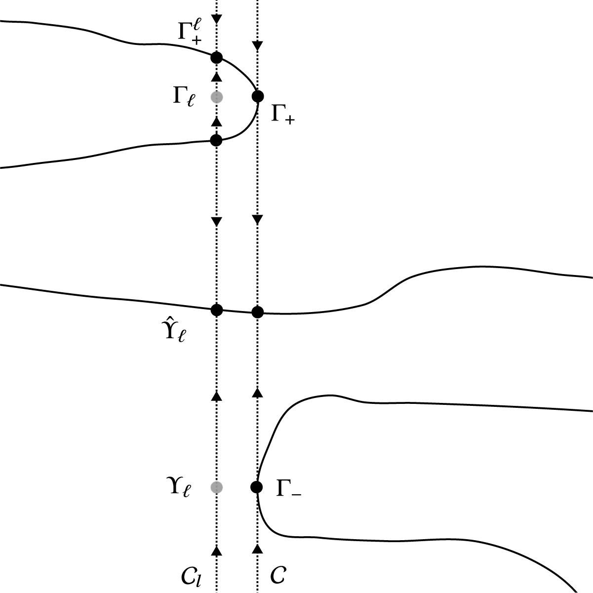
Figure 1 A schematic illustration of the situation in case (2) together with case (c). The horizontal axis is space of cones, the vertical axis the space of hypersurfaces asymptotic to the given cone where height corresponds to the order, $\preceq $
. The arrows represent directions of flow lines.
$\preceq $
. The arrows represent directions of flow lines.
In general, it may not be possible to perturb both elements in the pair to self-expanders – see Figure 1 for an illustration. However, one can always ensure that $\Gamma _+^\prime ,\Gamma _-^\prime $
are either self-expanders or expander mean convex hypersurfaces. For exapnder mean convex perturbations, invoking Propositions 2.2 and 3.6 yields self-expanders
$\Gamma _+^\prime ,\Gamma _-^\prime $
are either self-expanders or expander mean convex hypersurfaces. For exapnder mean convex perturbations, invoking Propositions 2.2 and 3.6 yields self-expanders $\hat {\Gamma }_+,\hat {\Gamma }_-\in \mathcal {E}(\mathcal {C}^\prime )$
along with relationships between the topologies of
$\hat {\Gamma }_+,\hat {\Gamma }_-\in \mathcal {E}(\mathcal {C}^\prime )$
along with relationships between the topologies of $\Gamma _\pm ^\prime $
and
$\Gamma _\pm ^\prime $
and $\hat {\Gamma }_\pm $
. However, to complete this argument, one must be able to control the relationship between the partial orders and direction of the expander mean curvature vectors of the initial perturbations which is a subtle issue. Specifically, one must know that
$\hat {\Gamma }_\pm $
. However, to complete this argument, one must be able to control the relationship between the partial orders and direction of the expander mean curvature vectors of the initial perturbations which is a subtle issue. Specifically, one must know that $\hat {\Gamma }_+\preceq \Gamma _+^\prime $
,
$\hat {\Gamma }_+\preceq \Gamma _+^\prime $
, $\Gamma _-^\prime \preceq \hat {\Gamma }_-$
, and
$\Gamma _-^\prime \preceq \hat {\Gamma }_-$
, and $\hat {\Gamma }_-\preceq \hat {\Gamma }_+$
, which do not, in general, hold. To overcome this, we prove a restricted result by requiring
$\hat {\Gamma }_-\preceq \hat {\Gamma }_+$
, which do not, in general, hold. To overcome this, we prove a restricted result by requiring $\Gamma _+$
and
$\Gamma _+$
and $\Gamma _-$
to be the greatest and least element of
$\Gamma _-$
to be the greatest and least element of $\mathcal {E}(\mathcal {C})$
– whose existence is shown in [Reference Bernstein and Wang9, Theorem 4.1].
$\mathcal {E}(\mathcal {C})$
– whose existence is shown in [Reference Bernstein and Wang9, Theorem 4.1].
Proposition 3.7. For $2\leq n\leq 6$
, let
$2\leq n\leq 6$
, let $\mathcal {C}$
be a degenerate
$\mathcal {C}$
be a degenerate $C^5$
-regular cone in
$C^5$
-regular cone in $\mathbb {R}^{n+1}$
such that
$\mathbb {R}^{n+1}$
such that $\mathcal {L}(\mathcal {C})$
is connected and, for some
$\mathcal {L}(\mathcal {C})$
is connected and, for some $m\in [1,n-1]$
,
$m\in [1,n-1]$
,
 $$\begin{align*}\lambda(\mathcal{C})<\lambda(\mathbb{S}^{m}\times\mathbb{R}^{n-m}). \end{align*}$$
If $\Gamma _+$
and
$\Gamma _+$
and $\Gamma _-$
are respectively the greatest and least element of
$\Gamma _-$
are respectively the greatest and least element of $\mathcal {E}(\mathcal {C})$
, that is,
$\mathcal {E}(\mathcal {C})$
, that is, $\Gamma _-\preceq \Gamma \preceq \Gamma _+$
for
$\Gamma _-\preceq \Gamma \preceq \Gamma _+$
for $\Gamma \in \mathcal {E}(\mathcal {C})$
, then the inclusions
$\Gamma \in \mathcal {E}(\mathcal {C})$
, then the inclusions $\mathfrak {i}^\pm \colon \Omega _\pm (\Gamma _\pm ) \to \Omega _\pm (\Gamma _\mp )$
induce homomorphisms
$\mathfrak {i}^\pm \colon \Omega _\pm (\Gamma _\pm ) \to \Omega _\pm (\Gamma _\mp )$
induce homomorphisms
 $$\begin{align*}\mathfrak{i}^\pm_* \colon H_k(\Omega_\pm(\Gamma_\pm)) \to H_k(\Omega_\pm(\Gamma_\mp)) \end{align*}$$
such that
-
1. When
$n-m\leq k\leq m$
, the maps
$\mathfrak {i}^\pm _*$
are bijective; -
2. When
$n-m-1=k\leq m$
, the maps
$\mathfrak {i}^\pm _*$
are injective; -
3. When
$n-m\leq k=m+1$
, the maps
$\mathfrak {i}^\pm _*$
are surjective.


Proof. First we show there is a sequence of nondegenerate $C^4$
-regular cones
$C^4$
-regular cones $\mathcal {C}_\ell \subset \mathbb {R}^{n+1}$
with link
$\mathcal {C}_\ell \subset \mathbb {R}^{n+1}$
with link $\mathcal {L}(\mathcal {C}_\ell )$
so that
$\mathcal {L}(\mathcal {C}_\ell )$
so that $\mathcal {L}(\mathcal {C}_\ell )\to \mathcal {L}(\mathcal {C})$
in
$\mathcal {L}(\mathcal {C}_\ell )\to \mathcal {L}(\mathcal {C})$
in $C^4(\mathbb {S}^n)$
and
$C^4(\mathbb {S}^n)$
and $\Gamma ^\ell _+\to \Gamma _+$
in
$\Gamma ^\ell _+\to \Gamma _+$
in $C^\infty _{loc}(\mathbb {R}^{n+1})$
, where
$C^\infty _{loc}(\mathbb {R}^{n+1})$
, where $\Gamma _+^\ell $
is the greatest element of
$\Gamma _+^\ell $
is the greatest element of $\mathcal {E}(\mathcal {C}_\ell )$
. In particular, for sufficiently large
$\mathcal {E}(\mathcal {C}_\ell )$
. In particular, for sufficiently large $\ell $
,
$\ell $
,
 $$ \begin{align} \lambda(\mathcal{C}_\ell)<\lambda(\mathcal{C})+\epsilon<\lambda(\mathbb{S}^m\times\mathbb{R}^{n-m}). \end{align} $$
To see this, first observe by [Reference Bernstein and Wang9, Theorem 4.1], one has $\Gamma _+$
is a stable self-expander. Let
$\Gamma _+$
is a stable self-expander. Let $\mathcal {K}$
denote the space of Jacobi fields on
$\mathcal {K}$
denote the space of Jacobi fields on $\Gamma _+$
that fix the infinity. Using standard spectral theory and the results of [Reference Bernstein4] – see also [Reference Bernstein and Wang7, Lemma 6.1] and [Reference Bernstein and Wang11, Proposition 3.2] – together with the connectedness of
$\Gamma _+$
that fix the infinity. Using standard spectral theory and the results of [Reference Bernstein4] – see also [Reference Bernstein and Wang7, Lemma 6.1] and [Reference Bernstein and Wang11, Proposition 3.2] – together with the connectedness of $\Gamma _+$
, it follows that
$\Gamma _+$
, it follows that $\dim \mathcal {K}\leq 1$
and every element of
$\dim \mathcal {K}\leq 1$
and every element of $\mathcal {K}$
either is identically
$\mathcal {K}$
either is identically $\mathbf {0}$
or has a sign and an asymptotic expansion with leading order term of the form
$\mathbf {0}$
or has a sign and an asymptotic expansion with leading order term of the form $\alpha r^{-n-1} e^{-r^2/4}$
, where
$\alpha r^{-n-1} e^{-r^2/4}$
, where $r=|\mathbf {x}|$
and
$r=|\mathbf {x}|$
and $\alpha $
is a function on
$\alpha $
is a function on $\mathcal {L}(\mathcal {C})$
.
$\mathcal {L}(\mathcal {C})$
.
We now appeal to results of [Reference Bernstein and Wang7] to perturb the asymptotic cone and the self-expander $\Gamma _+$
. First, recall that
$\Gamma _+$
. First, recall that $\mathcal {ACH}^4_n(\Gamma _+)$
denotes the space of
$\mathcal {ACH}^4_n(\Gamma _+)$
denotes the space of $C^4$
-asymptotically conical embeddings of
$C^4$
-asymptotically conical embeddings of $\Gamma _+$
into
$\Gamma _+$
into $\mathbb {R}^{n+1}$
, equipped with the weighted
$\mathbb {R}^{n+1}$
, equipped with the weighted $C^4$
norm with weight r – see [Reference Bernstein and Wang7, §3.2] for the precise definition. Following [Reference Bernstein and Wang7], say a
$C^4$
norm with weight r – see [Reference Bernstein and Wang7, §3.2] for the precise definition. Following [Reference Bernstein and Wang7], say a $C^3$
-regular cone
$C^3$
-regular cone $\mathcal {C}^{\prime }$
is nondegenerate if no self-expander asymptotic to
$\mathcal {C}^{\prime }$
is nondegenerate if no self-expander asymptotic to $\mathcal {C}^{\prime }$
admits a nontrivial Jacobi field – as shown in [Reference Bernstein and Wang7], such cones are generic in a suitable sense. With this in mind, we use [Reference Bernstein and Wang7, Theorem 7.1] to choose a sequence of
$\mathcal {C}^{\prime }$
admits a nontrivial Jacobi field – as shown in [Reference Bernstein and Wang7], such cones are generic in a suitable sense. With this in mind, we use [Reference Bernstein and Wang7, Theorem 7.1] to choose a sequence of $C^4$
-regular cones
$C^4$
-regular cones $\mathcal {C}_\ell $
along with
$\mathcal {C}_\ell $
along with $C^4$
-asymptotically conical hypersurfaces
$C^4$
-asymptotically conical hypersurfaces $\Gamma _\ell $
with nondegenerate asymptotic cone so that the
$\Gamma _\ell $
with nondegenerate asymptotic cone so that the $\mathcal {C}_{\ell }$
converge to
$\mathcal {C}_{\ell }$
converge to $\mathcal {C}$
and the
$\mathcal {C}$
and the $\Gamma _\ell $
converge
$\Gamma _\ell $
converge $\Gamma _+$
in
$\Gamma _+$
in $\mathcal {ACH}^4_n(\Gamma _+)$
. Here, we understand the convergence by identifying the
$\mathcal {ACH}^4_n(\Gamma _+)$
. Here, we understand the convergence by identifying the $\Gamma _\ell $
with the parameterizations given by the inverse of the nearest point projections onto
$\Gamma _\ell $
with the parameterizations given by the inverse of the nearest point projections onto $\Gamma _+$
which are elements of
$\Gamma _+$
which are elements of $\mathcal {ACH}^4_n(\Gamma _+)$
.
$\mathcal {ACH}^4_n(\Gamma _+)$
.
It follows from [Reference Bernstein and Wang7, Theorem 7.1] that the cones $\mathcal {C}_{\ell }$
and hypersurfaces
$\mathcal {C}_{\ell }$
and hypersurfaces $\Gamma _\ell $
can be chosen so that either:
$\Gamma _\ell $
can be chosen so that either:
-
1. If
$\mathcal {K}=\{\mathbf {0}\}$
, then
$\Gamma _\ell \in \mathcal {E}(\mathcal {C}_\ell )$
for each
$\ell $
; or; -
2. If
$\mathcal {K}\neq \{\mathbf {0}\}$
, then
$2\mathbf {H}_{\Gamma _\ell }-\mathbf {x}^\perp $
is nowhere vanishing and the pushforward of it by the nearest projection onto
$\Gamma _+$
is a nonzero element of
$\mathcal {K}$
.


If case (2) occurs, then one can modify the choice of cones in order to ensure that $2\mathbf {H}_{\Gamma _\ell }-\mathbf {x}^\perp $
points into
$2\mathbf {H}_{\Gamma _\ell }-\mathbf {x}^\perp $
points into $\Omega _+(\Gamma _\ell )$
– here, one chooses the boundary link of
$\Omega _+(\Gamma _\ell )$
– here, one chooses the boundary link of $\mathcal {L}(\mathcal {C}_\ell )$
in the obvious way compatible with that of
$\mathcal {L}(\mathcal {C}_\ell )$
in the obvious way compatible with that of $\mathcal {L}(\mathcal {C})$
. This ensures that for the choice of unit normal
$\mathcal {L}(\mathcal {C})$
. This ensures that for the choice of unit normal $\mathbf {n}_{\Gamma _\ell }$
on
$\mathbf {n}_{\Gamma _\ell }$
on $\Gamma _{\ell }$
that is compatible with the boundary link – that is, that points out of
$\Gamma _{\ell }$
that is compatible with the boundary link – that is, that points out of $\Omega _+(\Gamma _\ell )$
– one has
$\Omega _+(\Gamma _\ell )$
– one has $2H_{\Gamma _\ell }+\mathbf {x}\cdot \mathbf {n}_{\Gamma _\ell }>0$
. That is, we may either choose the
$2H_{\Gamma _\ell }+\mathbf {x}\cdot \mathbf {n}_{\Gamma _\ell }>0$
. That is, we may either choose the $\Gamma _\ell $
to all be self-expanders or to all be expander mean convex with expander mean curvature vector pointing into
$\Gamma _\ell $
to all be self-expanders or to all be expander mean convex with expander mean curvature vector pointing into $\Omega _+(\Gamma _\ell )$
.
$\Omega _+(\Gamma _\ell )$
.
In case (1), it is readily seen that the construction and the compactness properties of spaces of expanders [Reference Bernstein and Wang9, Proposition 4.4] ensure that the $\Gamma ^\ell _+$
converge smoothly on compact sets to
$\Gamma ^\ell _+$
converge smoothly on compact sets to $\Gamma _+$
. In case (2), by Proposition 2.2, the expander flow starting from
$\Gamma _+$
. In case (2), by Proposition 2.2, the expander flow starting from $\Gamma _\ell $
is contained in
$\Gamma _\ell $
is contained in $\Omega _+(\Gamma _\ell )$
and is asymptotic at time
$\Omega _+(\Gamma _\ell )$
and is asymptotic at time $\infty $
to a stable self-expander
$\infty $
to a stable self-expander $\hat {\Gamma }_\ell \in \mathcal {E}(\mathcal {C}_\ell )$
. As
$\hat {\Gamma }_\ell \in \mathcal {E}(\mathcal {C}_\ell )$
. As $\Gamma _\ell \preceq \hat {\Gamma }_\ell $
and
$\Gamma _\ell \preceq \hat {\Gamma }_\ell $
and $\Gamma _\ell \to \Gamma _+$
, invoking compactness again gives that the
$\Gamma _\ell \to \Gamma _+$
, invoking compactness again gives that the $\hat {\Gamma }_\ell $
converge, in
$\hat {\Gamma }_\ell $
converge, in $C^\infty _{loc}(\mathbb {R}^{n+1})$
, to a limit expander
$C^\infty _{loc}(\mathbb {R}^{n+1})$
, to a limit expander $\hat {\Gamma }\in \mathcal {E}(\mathcal {C})$
that satisfies
$\hat {\Gamma }\in \mathcal {E}(\mathcal {C})$
that satisfies $\Gamma _+\preceq \hat {\Gamma }$
. As
$\Gamma _+\preceq \hat {\Gamma }$
. As $\Gamma _+$
is the greatest element one must have
$\Gamma _+$
is the greatest element one must have $\Gamma _+=\hat {\Gamma }$
. The same reasoning ensures that, up to passing to a further subsequence, the greatest elements,
$\Gamma _+=\hat {\Gamma }$
. The same reasoning ensures that, up to passing to a further subsequence, the greatest elements, $\Gamma _+^\ell $
, of
$\Gamma _+^\ell $
, of $\mathcal {E}(\mathcal {C}_\ell )$
also converge to
$\mathcal {E}(\mathcal {C}_\ell )$
also converge to $\Gamma _+$
. This verifies the initial claim that we may find a sequence of cones
$\Gamma _+$
. This verifies the initial claim that we may find a sequence of cones $\mathcal {C}_\ell $
so that the greatest elements,
$\mathcal {C}_\ell $
so that the greatest elements, $\Gamma ^\ell _+$
, of
$\Gamma ^\ell _+$
, of $\mathcal {E}(\mathcal {C}_\ell )$
converge to
$\mathcal {E}(\mathcal {C}_\ell )$
converge to $\Gamma _+$
.
$\Gamma _+$
.
Using the sequence of cones, $\mathcal {C}_\ell $
, from the previous step and making the same argument with
$\mathcal {C}_\ell $
, from the previous step and making the same argument with $\Gamma _-$
in place of
$\Gamma _-$
in place of $\Gamma _+$
yields a sequence of
$\Gamma _+$
yields a sequence of $C^4$
-asymptotically conical hypersurfaces
$C^4$
-asymptotically conical hypersurfaces $\Upsilon _\ell $
with asymptotic cone
$\Upsilon _\ell $
with asymptotic cone $\mathcal {C}_\ell $
that converges to
$\mathcal {C}_\ell $
that converges to $\Gamma _-$
in
$\Gamma _-$
in $\mathcal {ACH}^4_n(\Gamma _-)$
and such that, up to passing to a subsequence, one of the following holds:
$\mathcal {ACH}^4_n(\Gamma _-)$
and such that, up to passing to a subsequence, one of the following holds:
-
(a)
$\Upsilon _\ell \in \mathcal {E}(\mathcal {C}_\ell )$
for each
$\ell $
; -
(b)
$2H_{\Upsilon _\ell }+\mathbf {x}\cdot \mathbf {n}_{\Upsilon _\ell }<0$
for each
$\ell $
; -
(c)
$2H_{\Upsilon _\ell }+\mathbf {x}\cdot \mathbf {n}_{\Upsilon _\ell }>0$
for each
$\ell $
.


Here, $\mathbf {n}_{\Upsilon _\ell }$
is the outward normal to
$\mathbf {n}_{\Upsilon _\ell }$
is the outward normal to $\Omega _+(\Upsilon _\ell )$
. Case (b) means the expander mean curvature vector points into
$\Omega _+(\Upsilon _\ell )$
. Case (b) means the expander mean curvature vector points into $\Omega _+(\Upsilon _\ell )$
and out of
$\Omega _+(\Upsilon _\ell )$
and out of $\Omega _-(\Upsilon _\ell )$
and case (c) means it points out of
$\Omega _-(\Upsilon _\ell )$
and case (c) means it points out of $\Omega _+(\Upsilon _\ell )$
and into
$\Omega _+(\Upsilon _\ell )$
and into $\Omega _-(\Upsilon _\ell )$
. Observe that three cases may occur rather than two as in the previous step, as we have already fixed the sequence of cones so we cannot specify whether the nowhere zero expander mean curvature vector points out of or into
$\Omega _-(\Upsilon _\ell )$
. Observe that three cases may occur rather than two as in the previous step, as we have already fixed the sequence of cones so we cannot specify whether the nowhere zero expander mean curvature vector points out of or into $\Omega _+(\Upsilon _\ell )$
only that one of the two situations holds for all
$\Omega _+(\Upsilon _\ell )$
only that one of the two situations holds for all $\ell $
.
$\ell $
.
When case (a) or (b) occurs, one argues as before to see the least elements $\Gamma ^\ell _-$
of
$\Gamma ^\ell _-$
of $\mathcal {E}(\mathcal {C}_\ell )$
converge smoothly on compact sets to
$\mathcal {E}(\mathcal {C}_\ell )$
converge smoothly on compact sets to $\Gamma _-$
. By [Reference Bernstein and Wang8, Proposition 3.3], there is a radius
$\Gamma _-$
. By [Reference Bernstein and Wang8, Proposition 3.3], there is a radius $R>1$
so that
$R>1$
so that $\Omega _\pm (\Gamma ^\ell _-)\cap \bar {B}_R$
is a deformation retract of
$\Omega _\pm (\Gamma ^\ell _-)\cap \bar {B}_R$
is a deformation retract of $\Omega _\pm (\Gamma ^\ell _-)$
for each
$\Omega _\pm (\Gamma ^\ell _-)$
for each $\ell $
. The nature of convergence ensures that
$\ell $
. The nature of convergence ensures that $\Omega _\pm (\Gamma ^\ell _-)$
is homotopy equivalent to
$\Omega _\pm (\Gamma ^\ell _-)$
is homotopy equivalent to $\Omega _\pm (\Gamma _-)$
for sufficiently large
$\Omega _\pm (\Gamma _-)$
for sufficiently large $\ell $
. Likewise,
$\ell $
. Likewise, $\Omega _\pm (\Gamma ^\ell _+)$
is homotopy equivalent to
$\Omega _\pm (\Gamma ^\ell _+)$
is homotopy equivalent to $\Omega _\pm (\Gamma _+)$
for large
$\Omega _\pm (\Gamma _+)$
for large $\ell $
. The claim follows from this and Theorem 3.1 for
$\ell $
. The claim follows from this and Theorem 3.1 for $\Gamma _-^\ell \preceq \Gamma ^\ell _+$
(in view of (3.4)).
$\Gamma _-^\ell \preceq \Gamma ^\ell _+$
(in view of (3.4)).
It remains only to deal with case (c). We refer to Figure 1. Fix a large $\ell $
so that
$\ell $
so that $\Omega _\pm (\Gamma _+^\ell )$
and
$\Omega _\pm (\Gamma _+^\ell )$
and $\Omega _\pm (\Upsilon _\ell )$
are homotopy equivalent to
$\Omega _\pm (\Upsilon _\ell )$
are homotopy equivalent to $\Omega _\pm (\Gamma _+)$
and
$\Omega _\pm (\Gamma _+)$
and $\Omega _\pm (\Gamma _-)$
, respectively. Observing
$\Omega _\pm (\Gamma _-)$
, respectively. Observing $\Upsilon _\ell \preceq \Gamma _+^\ell $
, we then let
$\Upsilon _\ell \preceq \Gamma _+^\ell $
, we then let $\mathfrak {i}_\ell ^+\colon \Omega _+(\Gamma _+^\ell )\to \Omega _+(\Upsilon _\ell )$
and
$\mathfrak {i}_\ell ^+\colon \Omega _+(\Gamma _+^\ell )\to \Omega _+(\Upsilon _\ell )$
and $\mathfrak {i}_\ell ^-\colon \Omega _-(\Upsilon _\ell )\to \Omega _-(\Gamma _+^\ell )$
be the inclusion maps. Hence, it suffices to show the induced maps
$\mathfrak {i}_\ell ^-\colon \Omega _-(\Upsilon _\ell )\to \Omega _-(\Gamma _+^\ell )$
be the inclusion maps. Hence, it suffices to show the induced maps $(\mathfrak {i}_\ell ^+)_* \colon H_k(\Omega _+(\Gamma _+^\ell ))\to H_k(\Omega _+(\Upsilon _\ell ))$
and
$(\mathfrak {i}_\ell ^+)_* \colon H_k(\Omega _+(\Gamma _+^\ell ))\to H_k(\Omega _+(\Upsilon _\ell ))$
and $(\mathfrak {i}^-_\ell )_* \colon H_k(\Omega _-(\Upsilon _\ell ))\to H_k(\Omega _-(\Gamma ^\ell _+))$
are bijective when
$(\mathfrak {i}^-_\ell )_* \colon H_k(\Omega _-(\Upsilon _\ell ))\to H_k(\Omega _-(\Gamma ^\ell _+))$
are bijective when $n-m\leq k\leq m$
, are injective when
$n-m\leq k\leq m$
, are injective when $n-m-1=k\leq m$
, and are surjective when
$n-m-1=k\leq m$
, and are surjective when $n-m\leq k=m+1$
.
$n-m\leq k=m+1$
.
By Proposition 2.2, there is a strongly regular strictly monotone expander weak flow $\mathcal {S}_\ell $
asymptotic to
$\mathcal {S}_\ell $
asymptotic to $\mathcal {C}_\ell $
with initial data
$\mathcal {C}_\ell $
with initial data $\Omega _+(\Upsilon _\ell )$
, and the flow converges smoothly to a closed set with smooth boundary
$\Omega _+(\Upsilon _\ell )$
, and the flow converges smoothly to a closed set with smooth boundary $\hat {\Upsilon }_\ell \in \mathcal {E}(\mathcal {C}_\ell )$
satisfying
$\hat {\Upsilon }_\ell \in \mathcal {E}(\mathcal {C}_\ell )$
satisfying ${\Upsilon }_{\ell }\preceq \hat {\Upsilon }_\ell \preceq \Gamma _+^\ell $
. In particular, for large t, the time-t slice of the flow line is smoothly isotopic to
${\Upsilon }_{\ell }\preceq \hat {\Upsilon }_\ell \preceq \Gamma _+^\ell $
. In particular, for large t, the time-t slice of the flow line is smoothly isotopic to $\hat {\Upsilon }_\ell $
. By construction,
$\hat {\Upsilon }_\ell $
. By construction,
 $$\begin{align*}\lambda(\Upsilon_\ell)<\lambda(\Gamma_-)+\epsilon=\lambda(\mathcal{C})+\epsilon<\lambda(\mathbb{S}^m\times\mathbb{R}^{n-m}), \end{align*}$$
and so the Huisken monotonicity [Reference Huisken24] implies, for $X_0\in \mathbb {R}^{n+1}\times (0,\infty )$
, that
$X_0\in \mathbb {R}^{n+1}\times (0,\infty )$
, that
 $$\begin{align*}\theta(\mathcal{M}_\ell,X_0)\leq\lambda(\mathbb{S}^{m+1}\times\mathbb{R}^{n-m-1}), \end{align*}$$
where $\mathcal {M}_\ell $
is the measure flow associated with
$\mathcal {M}_\ell $
is the measure flow associated with $\mathcal {S}_\ell $
– see Item (5) of Definition 2.1. The result follows by combining Proposition 3.6 applied to
$\mathcal {S}_\ell $
– see Item (5) of Definition 2.1. The result follows by combining Proposition 3.6 applied to $\mathcal {S}_\ell $
which yields relations between the topologies of
$\mathcal {S}_\ell $
which yields relations between the topologies of $\Upsilon _\ell \preceq \hat {\Upsilon }_\ell $
together with Theorem 3.1 which gives relationships between the topologies of
$\Upsilon _\ell \preceq \hat {\Upsilon }_\ell $
together with Theorem 3.1 which gives relationships between the topologies of $\hat {\Upsilon }_\ell \preceq \Gamma ^\ell _+$
. Observe that Theorem 3.1 applies to
$\hat {\Upsilon }_\ell \preceq \Gamma ^\ell _+$
. Observe that Theorem 3.1 applies to $\hat {\Upsilon }_\ell \preceq \Gamma _\ell ^+$
because of (3.4) and because the
$\hat {\Upsilon }_\ell \preceq \Gamma _\ell ^+$
because of (3.4) and because the $\mathcal {C}_\ell $
were chosen to be nondegenerate.
$\mathcal {C}_\ell $
were chosen to be nondegenerate.
4 Density of minimal cones
In this section, we prove the main results about densities of minimal cones. We continue to use the conventions of Section 3. We will repeatedly invoke the following auxiliary lemma about properties of the greatest and least element of $\mathcal {E}(\mathcal {C})$
for a minimal cone
$\mathcal {E}(\mathcal {C})$
for a minimal cone $\mathcal {C}$
– see [Reference Bernstein and Wang9, Theorem 4.1] for the existence of those elements.
$\mathcal {C}$
– see [Reference Bernstein and Wang9, Theorem 4.1] for the existence of those elements.
Lemma 4.1. For $3\leq n\leq 6$
, let
$3\leq n\leq 6$
, let $\mathcal {C}\subset \mathbb {R}^{n+1}$
be a non-flat regular minimal cone. If
$\mathcal {C}\subset \mathbb {R}^{n+1}$
be a non-flat regular minimal cone. If $\Sigma _+$
and
$\Sigma _+$
and $\Sigma _-$
are respectively the greatest and least element of
$\Sigma _-$
are respectively the greatest and least element of $\mathcal {E}(\mathcal {C})$
, then the following is true:
$\mathcal {E}(\mathcal {C})$
, then the following is true:
-
1.
$\mathcal {L}(\mathcal {C})$
is connected; -
2.
$\Sigma _\pm \subset \mathrm {int}(\Omega _\pm (\mathcal {C}))$
; -
3. The projections
$\Pi ^\pm \colon \Sigma _\pm \to \mathbb {S}^n$
given by are diffeomorphisms onto their images
$$\begin{align*}\Pi^\pm(p)=\frac{\mathbf{x}(p)}{|\mathbf{x}(p)|} \end{align*}$$
$\mathrm {int}(\Omega _\pm (\mathcal {C}))\cap \mathbb {S}^n$
;
-
4. The sets
$\Omega _\mp (\Sigma _\pm )$
are star-shaped relative to
$\mathbf {0}$
; -
5. The inclusions of
$\Sigma _\pm $
into
$\mathrm {int}(\Omega _\pm (\mathcal {C}))$
are deformation retracts.


Proof. First of all, because $\mathcal {L}(\mathcal {C})$
is a smooth minimal hypersurface in
$\mathcal {L}(\mathcal {C})$
is a smooth minimal hypersurface in $\mathbb {S}^n$
, the Frankel theorem [Reference Frankel18] ensures it has only one connected component.
$\mathbb {S}^n$
, the Frankel theorem [Reference Frankel18] ensures it has only one connected component.
As $\mathcal {C}$
is a non-flat regular minimal cone, it is E-stationary and singular. It follows from the regularity theory for area-minimizing hypersurfaces that
$\mathcal {C}$
is a non-flat regular minimal cone, it is E-stationary and singular. It follows from the regularity theory for area-minimizing hypersurfaces that $\mathcal {C}$
cannot be E-minimizing. Thus,
$\mathcal {C}$
cannot be E-minimizing. Thus, $\Sigma _\pm \subset \mathrm {int}(\Omega _\pm (\mathcal {C}))$
, as otherwise, one may use a minimization procedure (see [Reference Ilmanen31, pp. 13–14] and [Reference Ding17, §6] or [Reference Bernstein and Wang9, §4]) to construct a
$\Sigma _\pm \subset \mathrm {int}(\Omega _\pm (\mathcal {C}))$
, as otherwise, one may use a minimization procedure (see [Reference Ilmanen31, pp. 13–14] and [Reference Ding17, §6] or [Reference Bernstein and Wang9, §4]) to construct a $\Sigma ^\prime _\pm \in \mathcal {E}(\mathcal {C})$
so that
$\Sigma ^\prime _\pm \in \mathcal {E}(\mathcal {C})$
so that $\Sigma ^\prime _\pm $
is contained in the interior of
$\Sigma ^\prime _\pm $
is contained in the interior of $\Omega _\pm (\Sigma _\pm )\cap \Omega _\pm (\mathcal {C})$
, either contradicting
$\Omega _\pm (\Sigma _\pm )\cap \Omega _\pm (\mathcal {C})$
, either contradicting $\Sigma _+$
being the greatest element or
$\Sigma _+$
being the greatest element or $\Sigma _-$
being the least.
$\Sigma _-$
being the least.
Next, we show $\sqrt {t_1}\Sigma _+\preceq \sqrt {t_2}\Sigma _+$
for
$\sqrt {t_1}\Sigma _+\preceq \sqrt {t_2}\Sigma _+$
for $0<t_1<t_2$
, which implies
$0<t_1<t_2$
, which implies $\mathbf {H}_{\Sigma _+}$
vanishes nowhere and points into
$\mathbf {H}_{\Sigma _+}$
vanishes nowhere and points into $\Omega _+(\Sigma _+)$
. To see this, we let
$\Omega _+(\Sigma _+)$
. To see this, we let $\delta =t_2-t_1$
and consider two mean curvature flows
$\delta =t_2-t_1$
and consider two mean curvature flows $\mathcal {M}=\{\sqrt {t}\Sigma _+\}_{t>0}$
and
$\mathcal {M}=\{\sqrt {t}\Sigma _+\}_{t>0}$
and $\mathcal {M}^\prime =\{\sqrt {t+\delta }\Sigma _+\}_{t>0}$
. As
$\mathcal {M}^\prime =\{\sqrt {t+\delta }\Sigma _+\}_{t>0}$
. As $\Omega _+(\sqrt {\delta }\Sigma _+)\subset \mathrm {int}(\Omega _+(\mathcal {C}))$
, the continuity of flows ensures that, for
$\Omega _+(\sqrt {\delta }\Sigma _+)\subset \mathrm {int}(\Omega _+(\mathcal {C}))$
, the continuity of flows ensures that, for $t>0$
small,
$t>0$
small, $\Omega _+(\sqrt {t+\delta }\Sigma _+)\cap \partial B_{2R}$
is contained in the interior of
$\Omega _+(\sqrt {t+\delta }\Sigma _+)\cap \partial B_{2R}$
is contained in the interior of $\Omega _+(\sqrt {t}\Sigma _+)\cap \partial B_{2R}$
. Suppose s is the first time in
$\Omega _+(\sqrt {t}\Sigma _+)\cap \partial B_{2R}$
. Suppose s is the first time in $(0,t_1]$
such that this fails. As
$(0,t_1]$
such that this fails. As $\Sigma _+$
is
$\Sigma _+$
is $C^2$
-asymptotic to
$C^2$
-asymptotic to $\mathcal {C}$
, there is a radius
$\mathcal {C}$
, there is a radius $R>1$
so that
$R>1$
so that $\sqrt {t+\delta }\Sigma _+\setminus B_{2R}$
can be written as an almost flat normal graph of a function
$\sqrt {t+\delta }\Sigma _+\setminus B_{2R}$
can be written as an almost flat normal graph of a function $u(t,\cdot )$
over (a subset of)
$u(t,\cdot )$
over (a subset of) $\sqrt {t}\Sigma _+$
for
$\sqrt {t}\Sigma _+$
for $0\leq t\leq t_1$
. A straightforward, but tedious, computation gives that u satisfies a uniformly parabolic equation with bounded coefficients. As
$0\leq t\leq t_1$
. A straightforward, but tedious, computation gives that u satisfies a uniformly parabolic equation with bounded coefficients. As $u\leq 0$
on the parabolic boundary, the strict maximum principle on noncompact regions – for example, Theorem 10 and Theorem 7 in [Reference Protter and Weinberger34, Chapter 3]Footnote 3 – implies
$u\leq 0$
on the parabolic boundary, the strict maximum principle on noncompact regions – for example, Theorem 10 and Theorem 7 in [Reference Protter and Weinberger34, Chapter 3]Footnote 3 – implies $u<0$
in the interior. That is, the restriction of
$u<0$
in the interior. That is, the restriction of $\mathcal {M}$
to
$\mathcal {M}$
to $(\mathbb {R}^{n+1}\setminus \bar {B}_{2R})\times (0,s]$
is disjoint from
$(\mathbb {R}^{n+1}\setminus \bar {B}_{2R})\times (0,s]$
is disjoint from $\mathcal {M}^\prime $
. Thus, there is a time
$\mathcal {M}^\prime $
. Thus, there is a time $s^\prime \in (0,s]$
so that the restriction of
$s^\prime \in (0,s]$
so that the restriction of $\mathcal {M}$
to
$\mathcal {M}$
to $(0,s^\prime )$
lies on one side of
$(0,s^\prime )$
lies on one side of $\mathcal {M}^\prime $
and
$\mathcal {M}^\prime $
and $\mathcal {M}$
touches
$\mathcal {M}$
touches $\mathcal {M}^\prime $
at a point in
$\mathcal {M}^\prime $
at a point in $\bar {B}_{2R}$
at time
$\bar {B}_{2R}$
at time $s^\prime $
, which violates the strict maximum principle on compact regions. That is,
$s^\prime $
, which violates the strict maximum principle on compact regions. That is, $\sqrt {t+\delta }\Sigma _+\cap \sqrt {t}\Sigma _+\cap \partial B_{2R}=\emptyset $
for
$\sqrt {t+\delta }\Sigma _+\cap \sqrt {t}\Sigma _+\cap \partial B_{2R}=\emptyset $
for $t\in (0,t_1]$
. The claim follows from the strict maximum principle.
$t\in (0,t_1]$
. The claim follows from the strict maximum principle.
Swapping the orientation, the arguments above imply $\mathbf {H}_{\Sigma _-}$
vanishes nowhere and points into
$\mathbf {H}_{\Sigma _-}$
vanishes nowhere and points into $\Omega _-(\Sigma _-)$
. The expander equation (2.1) implies
$\Omega _-(\Sigma _-)$
. The expander equation (2.1) implies $\mathbf {x}\cdot \mathbf {n}_{\Sigma _+}>0$
and
$\mathbf {x}\cdot \mathbf {n}_{\Sigma _+}>0$
and $\mathbf {x}\cdot \mathbf {n}_{\Sigma _-}<0$
, where
$\mathbf {x}\cdot \mathbf {n}_{\Sigma _-}<0$
, where $\mathbf {n}_{\Sigma _\pm }$
is the outward normal to
$\mathbf {n}_{\Sigma _\pm }$
is the outward normal to $\Omega _+(\Sigma _\pm )$
. It follows from [Reference Bernstein and Wang6, Proposition 5.1] that the projection
$\Omega _+(\Sigma _\pm )$
. It follows from [Reference Bernstein and Wang6, Proposition 5.1] that the projection $\Pi ^\pm \colon \Sigma _\pm \to \mathbb {S}^n$
is a diffeomorphism onto its image, and the image is
$\Pi ^\pm \colon \Sigma _\pm \to \mathbb {S}^n$
is a diffeomorphism onto its image, and the image is $\mathrm {int}(\Omega _\pm (\mathcal {C}))\cap \mathbb {S}^n$
. This also implies that
$\mathrm {int}(\Omega _\pm (\mathcal {C}))\cap \mathbb {S}^n$
. This also implies that $\Omega _\mp (\Sigma _\pm )$
is star-shaped relative to
$\Omega _\mp (\Sigma _\pm )$
is star-shaped relative to $\mathbf {0}$
and that the inclusions of
$\mathbf {0}$
and that the inclusions of $\Sigma _\pm $
into
$\Sigma _\pm $
into $\mathrm {int}(\Omega _\pm (\mathcal {C}))$
are deformation retracts and so completes the proof.
$\mathrm {int}(\Omega _\pm (\mathcal {C}))$
are deformation retracts and so completes the proof.
Theorem 1.1 follows from the proposition below.
Proposition 4.2. For $3\leq n\leq 6$
, let
$3\leq n\leq 6$
, let $\mathcal {C}$
be a regular minimal cone in
$\mathcal {C}$
be a regular minimal cone in $\mathbb {R}^{n+1}$
with
$\mathbb {R}^{n+1}$
with
 $$\begin{align*}\lambda(\mathcal{C})<\lambda(\mathbb{S}^{n-1}\times\mathbb{R}). \end{align*}$$
Then, for $\Sigma \in \mathcal {E}(\mathcal {C})$
, both
$\Sigma \in \mathcal {E}(\mathcal {C})$
, both $\Omega _+(\Sigma )$
and
$\Omega _+(\Sigma )$
and $\Omega _-(\Sigma )$
are contractible. This means
$\Omega _-(\Sigma )$
are contractible. This means $\Sigma $
and both components of
$\Sigma $
and both components of $\mathbb {S}^n\setminus \mathcal {L}(\mathcal {C})$
are contractible.
$\mathbb {S}^n\setminus \mathcal {L}(\mathcal {C})$
are contractible.
Remark 4.3. The fact that the two components of $\mathbb {S}^n\setminus \mathcal {L}(\mathcal {C})$
are contractible implies
$\mathbb {S}^n\setminus \mathcal {L}(\mathcal {C})$
are contractible implies $\mathcal {L}(\mathcal {C})$
is a homology sphere, but cannot rule out the presence of torsion elements in the fundamental group when
$\mathcal {L}(\mathcal {C})$
is a homology sphere, but cannot rule out the presence of torsion elements in the fundamental group when $n\geq 4$
.
$n\geq 4$
.
Proof of Proposition 4.2
By the maximum principle, if $\mathcal {C}$
is flat, then the only self-expander asymptotic to
$\mathcal {C}$
is flat, then the only self-expander asymptotic to $\mathcal {C}$
is a hyperplane and the claim holds trivially. Otherwise, let
$\mathcal {C}$
is a hyperplane and the claim holds trivially. Otherwise, let $\Sigma _+$
and
$\Sigma _+$
and $\Sigma _-$
be respectively the greatest and least element of
$\Sigma _-$
be respectively the greatest and least element of $\mathcal {E}(\mathcal {C})$
. By Lemma 4.1,
$\mathcal {E}(\mathcal {C})$
. By Lemma 4.1, $\mathcal {L}(\mathcal {C})$
is connected, and both
$\mathcal {L}(\mathcal {C})$
is connected, and both $\Omega _-(\Sigma _+)$
and
$\Omega _-(\Sigma _+)$
and $\Omega _+(\Sigma _-)$
are star-shaped relative to
$\Omega _+(\Sigma _-)$
are star-shaped relative to $\mathbf {0}$
and so are contractible. Combined with [Reference Bernstein and Wang9, Theorem 1.1], it follows that, for
$\mathbf {0}$
and so are contractible. Combined with [Reference Bernstein and Wang9, Theorem 1.1], it follows that, for $\Sigma \in \mathcal {E}(\mathcal {C})$
, both
$\Sigma \in \mathcal {E}(\mathcal {C})$
, both $\Omega _-(\Sigma )$
and
$\Omega _-(\Sigma )$
and $\Omega _+(\Sigma )$
are contractible. Furthermore, by Lemma 4.1, if
$\Omega _+(\Sigma )$
are contractible. Furthermore, by Lemma 4.1, if $\omega _\pm =\mathrm {int}(\Omega _\pm (\mathcal {C}))\cap \mathbb {S}^n$
, then both
$\omega _\pm =\mathrm {int}(\Omega _\pm (\mathcal {C}))\cap \mathbb {S}^n$
, then both $\Sigma _\pm $
and
$\Sigma _\pm $
and $\omega _\pm $
are homotopy equivalent to
$\omega _\pm $
are homotopy equivalent to $\Omega _\pm (\Sigma _\pm )$
, and thus, both
$\Omega _\pm (\Sigma _\pm )$
, and thus, both $\Sigma _\pm $
and
$\Sigma _\pm $
and $\omega _\pm $
are contractible. Finally, by [Reference Bernstein and Wang9, Theorem 1.1], every
$\omega _\pm $
are contractible. Finally, by [Reference Bernstein and Wang9, Theorem 1.1], every $\Sigma \in \mathcal {E}(\mathcal {C})$
is diffeomorphic to
$\Sigma \in \mathcal {E}(\mathcal {C})$
is diffeomorphic to $\Sigma _+$
and so is contractible.
$\Sigma _+$
and so is contractible.
Theorem 1.2 follows from the proposition below.
Proposition 4.4. For $3\leq n\leq 6$
, let
$3\leq n\leq 6$
, let $\mathcal {C}$
be a regular minimal cone in
$\mathcal {C}$
be a regular minimal cone in $\mathbb {R}^{n+1}$
with
$\mathbb {R}^{n+1}$
with
 $$\begin{align*}\lambda(\mathcal{C})<\lambda(\mathbb{S}^{n-2}\times\mathbb{R}^2). \end{align*}$$
If $\Sigma _+$
and
$\Sigma _+$
and $\Sigma _-$
are respectively the greatest and least element of
$\Sigma _-$
are respectively the greatest and least element of $\mathcal {E}(\mathcal {C})$
, then, for
$\mathcal {E}(\mathcal {C})$
, then, for $k\geq 0$
,
$k\geq 0$
,
 $$\begin{align*}\tilde{H}_k(\Omega_\mp(\Sigma_\pm))=\tilde{H}_k(\Omega_\pm(\Sigma_\pm))=\{0\}. \end{align*}$$
This means $\Sigma _+$
,
$\Sigma _+$
, $\Sigma _-$
, and the two components of
$\Sigma _-$
, and the two components of $\mathbb {S}^n\setminus \mathcal {L}(\mathcal {C})$
are all homology balls. In particular,
$\mathbb {S}^n\setminus \mathcal {L}(\mathcal {C})$
are all homology balls. In particular, $\mathcal {L}(\mathcal {C})$
is a homology sphere, and when
$\mathcal {L}(\mathcal {C})$
is a homology sphere, and when $n=3$
, the cone
$n=3$
, the cone $\mathcal {C}$
is flat.
$\mathcal {C}$
is flat.
Proof. If $\mathcal {C}$
is flat, then so is
$\mathcal {C}$
is flat, then so is $\Sigma _\pm $
. Otherwise, by Lemma 4.1,
$\Sigma _\pm $
. Otherwise, by Lemma 4.1, $\mathcal {L}(\mathcal {C})$
is connected and
$\mathcal {L}(\mathcal {C})$
is connected and $\Omega _\mp (\Sigma _\pm )$
are star-shaped relative to
$\Omega _\mp (\Sigma _\pm )$
are star-shaped relative to $\mathbf {0}$
. In particular, it follows that
$\mathbf {0}$
. In particular, it follows that $\Omega _\mp (\Sigma _\pm )$
are homotopy equivalent to
$\Omega _\mp (\Sigma _\pm )$
are homotopy equivalent to $B^{n+1}_1$
and so have trivial reduced homology groups.
$B^{n+1}_1$
and so have trivial reduced homology groups.
Likewise, if $\omega _\pm =\mathrm {int}(\Omega _\pm (\mathcal {C}))\cap \mathbb {S}^n$
, then
$\omega _\pm =\mathrm {int}(\Omega _\pm (\mathcal {C}))\cap \mathbb {S}^n$
, then $\Omega _\pm (\Sigma _\pm )$
is homotopy equivalent to
$\Omega _\pm (\Sigma _\pm )$
is homotopy equivalent to $\omega _\pm $
, and so, for
$\omega _\pm $
, and so, for $k\geq 0$
,
$k\geq 0$
,
 $$\begin{align*}H_k(\Omega_\pm(\Sigma_\pm))\cong H_k(\omega_\pm). \end{align*}$$
In particular, by the Alexander duality theorem – for example, [Reference Hatcher20, Theorem 3.44] – one immediately has
 $$\begin{align*}H_{n+1}(\Omega_\pm(\Sigma_\pm))\cong H_n(\Omega_\pm(\Sigma_\pm)) \cong H_{n-1}(\Omega_\pm(\Sigma_\pm))\cong \{0\}. \end{align*}$$
By Theorem 3.1 and Proposition 3.7, for $2\leq k\leq n-2$
, one has
$2\leq k\leq n-2$
, one has $H_k(\Omega _\pm (\Sigma _\pm ))$
is isomorphic to
$H_k(\Omega _\pm (\Sigma _\pm ))$
is isomorphic to $H_k(\Omega _\pm (\Sigma _\mp ))$
and so is trivial (this is vacuous for
$H_k(\Omega _\pm (\Sigma _\mp ))$
and so is trivial (this is vacuous for $n=3$
). Moreover, for
$n=3$
). Moreover, for $1=k\leq n-2$
, one has
$1=k\leq n-2$
, one has $H_1(\Omega _\pm (\Sigma _\pm ))$
is isomorphic to a subgroup of
$H_1(\Omega _\pm (\Sigma _\pm ))$
is isomorphic to a subgroup of $H_1(\Omega _\pm (\Sigma _\mp ))$
. As
$H_1(\Omega _\pm (\Sigma _\mp ))$
. As $H_1(\Omega _\pm (\Sigma _\mp ))$
is trivial, so is
$H_1(\Omega _\pm (\Sigma _\mp ))$
is trivial, so is $H_1(\Omega _\pm (\Sigma _\pm ))$
. It follows that
$H_1(\Omega _\pm (\Sigma _\pm ))$
. It follows that $\Omega _\pm (\Sigma _\pm )$
is a homology ball. Furthermore, by Lemma 4.1, both
$\Omega _\pm (\Sigma _\pm )$
is a homology ball. Furthermore, by Lemma 4.1, both $\Sigma _\pm $
and
$\Sigma _\pm $
and $\omega _\pm $
are homotopy equivalent to
$\omega _\pm $
are homotopy equivalent to $\Omega _\pm (\Sigma _\pm )$
and so are homology balls.
$\Omega _\pm (\Sigma _\pm )$
and so are homology balls.
To complete the proof, observe that, by the Mayer–Vietoris sequence (e.g., [Reference Hatcher20, p. 149]), as both $\omega _+$
and
$\omega _+$
and $\omega _-$
are homology balls,
$\omega _-$
are homology balls, $\mathcal {L}(\mathcal {C})$
is a homology sphere. When
$\mathcal {L}(\mathcal {C})$
is a homology sphere. When $n=3$
, the link
$n=3$
, the link $\mathcal {L}(\mathcal {C})$
is a surface that is a homology sphere and so, by the classification of surfaces, must be a topological
$\mathcal {L}(\mathcal {C})$
is a surface that is a homology sphere and so, by the classification of surfaces, must be a topological $\mathbb {S}^2$
. That is,
$\mathbb {S}^2$
. That is, $\mathcal {L}(\mathcal {C})$
is a minimal two-sphere in
$\mathcal {L}(\mathcal {C})$
is a minimal two-sphere in $\mathbb {S}^3$
and so, by results of Almgren [Reference Almgren2], must be totally geodesic; in this case,
$\mathbb {S}^3$
and so, by results of Almgren [Reference Almgren2], must be totally geodesic; in this case, $\mathcal {C}$
is flat.
$\mathcal {C}$
is flat.
We also obtain a weaker topological restriction under weaker entropy bounds.
Proposition 4.5. For $5\leq n\leq 6$
, let
$5\leq n\leq 6$
, let $\mathcal {C}$
be a regular minimal cone in
$\mathcal {C}$
be a regular minimal cone in $\mathbb {R}^{n+1}$
with
$\mathbb {R}^{n+1}$
with
 $$\begin{align*}\lambda(\mathcal{C})<\lambda (\mathbb{S}^{n-3}\times \mathbb{R}^{3}). \end{align*}$$
If $\Sigma _+$
and
$\Sigma _+$
and $\Sigma _-$
are respectively the greatest and least elements of
$\Sigma _-$
are respectively the greatest and least elements of $\mathcal {E}(\mathcal {C})$
, then the following is true:
$\mathcal {E}(\mathcal {C})$
, then the following is true:
-
1.
$\Omega _\mp (\Sigma _\pm )$
is a homology ball; -
2. When
$k\neq 1, n-2$
, one has
$\tilde {H}_k(\Omega _\pm (\Sigma _\pm ))=\{0\}$
. Otherwise,
$\tilde {H}_k(\Omega _\pm (\Sigma _\pm ))$
is a torsion-free group.


This means that when $k\neq 1,n-2$
, one has
$k\neq 1,n-2$
, one has $\tilde {H}_k(\Sigma _\pm )=\{0\}$
, and otherwise,
$\tilde {H}_k(\Sigma _\pm )=\{0\}$
, and otherwise, $\tilde {H}_k(\Sigma _\pm )$
is a torsion-free group. The same is true for the two components of
$\tilde {H}_k(\Sigma _\pm )$
is a torsion-free group. The same is true for the two components of $\mathbb {S}^n\setminus \mathcal {L}(\mathcal {C})$
. In particular,
$\mathbb {S}^n\setminus \mathcal {L}(\mathcal {C})$
. In particular, $H_k(\mathcal {L}(\mathcal {C}))=\{0\}$
when
$H_k(\mathcal {L}(\mathcal {C}))=\{0\}$
when $2\leq k\leq n-3$
and both
$2\leq k\leq n-3$
and both $H_1(\mathcal {L}(\mathcal {C}))$
and
$H_1(\mathcal {L}(\mathcal {C}))$
and $H_{n-2}(\mathcal {L}(\mathcal {C}))$
are torsion-free groups.
$H_{n-2}(\mathcal {L}(\mathcal {C}))$
are torsion-free groups.
Remark 4.6. Observe that this result applies to $\mathcal {C}_{2,2}\subset \mathbb {R}^6$
and gives the nearly optimal lower bound
$\mathcal {C}_{2,2}\subset \mathbb {R}^6$
and gives the nearly optimal lower bound $\Theta (\mathcal {C}_{2,2})\geq \lambda (\mathbb {S}^2)$
. Indeed, this estimate is sharp for any method that compares to the entropy of spheres because
$\Theta (\mathcal {C}_{2,2})\geq \lambda (\mathbb {S}^2)$
. Indeed, this estimate is sharp for any method that compares to the entropy of spheres because $\Theta (\mathcal {C}_{2,2})<\lambda (\mathbb {S}^1)$
– see Appendix A. However, it does not give any information about the density of
$\Theta (\mathcal {C}_{2,2})<\lambda (\mathbb {S}^1)$
– see Appendix A. However, it does not give any information about the density of $\mathcal {C}_{1,3}\subset \mathbb {R}^6$
even though direct computations give
$\mathcal {C}_{1,3}\subset \mathbb {R}^6$
even though direct computations give $\Theta (\mathcal {C}_{1,3})>\lambda (\mathbb {S}^1)>\Theta (\mathcal {C}_{2,2})$
. Moreover, even if one were able to strengthen the topological conclusions so that it gave information about
$\Theta (\mathcal {C}_{1,3})>\lambda (\mathbb {S}^1)>\Theta (\mathcal {C}_{2,2})$
. Moreover, even if one were able to strengthen the topological conclusions so that it gave information about $\mathcal {C}_{1,3}$
, the result would still not recover the bound
$\mathcal {C}_{1,3}$
, the result would still not recover the bound $\lambda (\mathbb {S}^1)$
and so would not be sharp in that regard. This is in contrast to Proposition 4.4 which applies to all generalized Simons’ cones.
$\lambda (\mathbb {S}^1)$
and so would not be sharp in that regard. This is in contrast to Proposition 4.4 which applies to all generalized Simons’ cones.
Proof of Proposition 4.5
Arguing as in the proof of Proposition 4.4 gives that $\Omega _\mp (\Sigma _\pm )$
has trivial reduced homology groups and when
$\Omega _\mp (\Sigma _\pm )$
has trivial reduced homology groups and when $2\leq k\leq n-3$
,
$2\leq k\leq n-3$
, $H_k(\Omega _\pm (\Sigma _\pm ))$
is trivial. By Lemma 4.1, if
$H_k(\Omega _\pm (\Sigma _\pm ))$
is trivial. By Lemma 4.1, if $\omega _\pm =\mathrm {int}(\Omega _\pm (\mathcal {C}))\cap \mathbb {S}^n$
, then
$\omega _\pm =\mathrm {int}(\Omega _\pm (\mathcal {C}))\cap \mathbb {S}^n$
, then $\Omega _\pm (\Sigma _\pm )$
and
$\Omega _\pm (\Sigma _\pm )$
and $\omega _\pm $
are homotopy equivalent and so have the same homology groups. Thus, combined with the Alexander duality (see [Reference Hatcher20, Theorem 3.44]), it follows that, for
$\omega _\pm $
are homotopy equivalent and so have the same homology groups. Thus, combined with the Alexander duality (see [Reference Hatcher20, Theorem 3.44]), it follows that, for $k\geq n-1$
, all
$k\geq n-1$
, all $H_k(\Omega _\pm (\Sigma _\pm ))$
are trivial. Likewise, by the universal coefficient theorem – for example, [Reference Hatcher20, Theorem 3.2] – both
$H_k(\Omega _\pm (\Sigma _\pm ))$
are trivial. Likewise, by the universal coefficient theorem – for example, [Reference Hatcher20, Theorem 3.2] – both $H_1(\Omega _\pm (\Sigma _\pm ))$
and
$H_1(\Omega _\pm (\Sigma _\pm ))$
and $H_{n-2}(\Omega _\pm (\Sigma _\pm ))$
are torsion-free. Hence, the claim on the homology of
$H_{n-2}(\Omega _\pm (\Sigma _\pm ))$
are torsion-free. Hence, the claim on the homology of $\Omega _\pm (\Sigma _\pm )$
holds. To complete the proof, observe that by Lemma 4.1, both
$\Omega _\pm (\Sigma _\pm )$
holds. To complete the proof, observe that by Lemma 4.1, both $\Sigma _\pm $
and
$\Sigma _\pm $
and $\omega _\pm $
are homotopy equivalent to
$\omega _\pm $
are homotopy equivalent to $\Omega _\pm (\Sigma _\pm )$
and so have the same homology groups as
$\Omega _\pm (\Sigma _\pm )$
and so have the same homology groups as $\Omega _\pm (\Sigma _\pm )$
. The description of the homology of
$\Omega _\pm (\Sigma _\pm )$
. The description of the homology of $\mathcal {L}(\mathcal {C})$
follows immediately from this and the Mayer–Vietoris sequence (see [Reference Hatcher20, p. 149]).
$\mathcal {L}(\mathcal {C})$
follows immediately from this and the Mayer–Vietoris sequence (see [Reference Hatcher20, p. 149]).
A Explicit densities and entropies
We give the explicit value of the densities of the generalized Simons’ cones as well as the entropies of spheres. We first remark that it follows from a computation of Stone [Reference Stone37, Appendix A] that
 $$ \begin{align*}\lambda(\mathbb{S}^n)=2 \sqrt{\pi}\left(\frac{n}{2e}\right)^{\frac{n}{2}}\frac{1}{\Gamma\left( \frac{n+1}{2}\right)}=\left(\frac{n}{2\pi e} \right)^{\frac{n}{2}} \sigma_n, \end{align*} $$
where $\sigma _n$
is the area of
$\sigma _n$
is the area of $\mathbb {S}^n$
and is given by
$\mathbb {S}^n$
and is given by
 $$ \begin{align*}\sigma_n=(n+1) \omega_{n+1}=(n+1)\frac{\pi^{\frac{n+1}{2}}}{\Gamma(\frac{n+3}{2})}. \end{align*} $$
Likewise, Ilmanen–White [Reference Ilmanen and White32] compute that for $\mathcal {C}_{m,l}\subset \mathbb {R}^{m+l+2}=\mathbb {R}^{n+1}$
,
$\mathcal {C}_{m,l}\subset \mathbb {R}^{m+l+2}=\mathbb {R}^{n+1}$
,
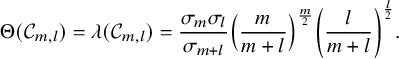 $$ \begin{align*}\Theta(\mathcal{C}_{m,l})=\lambda(\mathcal{C}_{m,l})=\frac{\sigma_m \sigma_l}{\sigma_{m+l}}\left( \frac{m}{m+l}\right)^{\frac{m}{2}} \left( \frac{l}{m+l}\right)^{\frac{l}{2}}. \end{align*} $$
As observed in [Reference Ilmanen and White32],
 $$ \begin{align*}\lim_{l\to \infty} \Theta(\mathcal{C}_{m,l})=\lambda(\mathbb{S}^m), \lim_{m\to \infty} =\Theta(\mathcal{C}_{m,l})=\lambda(\mathbb{S}^l) \end{align*} $$
and
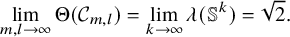 $$ \begin{align*}\lim_{m,l\to \infty} \Theta(\mathcal{C}_{m,l})=\lim_{k\to \infty} \lambda(\mathbb{S}^k)=\sqrt{2}. \end{align*} $$
The densities of generalized Simons’ cones in low dimensions is recorded in Table 1.
Table 1 Densities of generalized Simons’ cones.
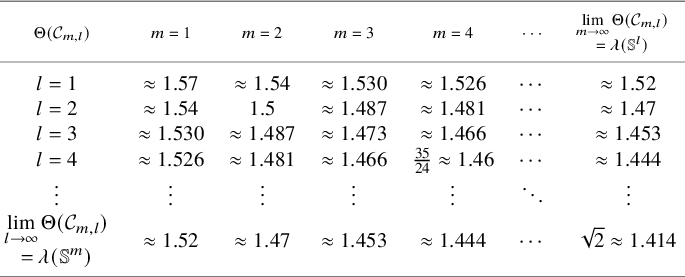
It is also convenient to set
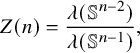 $$ \begin{align*}Z(n)=\frac{\lambda(\mathbb{S}^{n-2})}{\lambda(\mathbb{S}^{n-1})}, \end{align*} $$
which is the density lower bounds proved by Zhu in [Reference Zhu43]. We compare the densities of generalized Simons’ cones, $\mathcal {C}_{k, n-k-1}\subset \mathbb {R}^{n+1}$
for
$\mathcal {C}_{k, n-k-1}\subset \mathbb {R}^{n+1}$
for $3\leq n \leq 7$
and
$3\leq n \leq 7$
and $1\leq k \leq \lfloor \frac {n}{2}\rfloor $
with the bounds provided by Propositions 4.2, 4.4 and 4.5 and
$1\leq k \leq \lfloor \frac {n}{2}\rfloor $
with the bounds provided by Propositions 4.2, 4.4 and 4.5 and $Z(n)$
in Table 2.
$Z(n)$
in Table 2.
Table 2 Densities of generalized Simons’ cones and theoretical bounds.
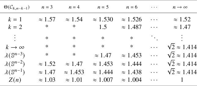
Finally, we compare the bounds using entropy of spheres with the universal bounds provided by [Reference Cheng, Li and Yau15]. Let
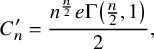 $$ \begin{align*}C_n^{\prime}=\frac{n^{\frac{n}{2}} e \Gamma\left(\frac{n}{2},1\right)}{2}, \end{align*} $$
where $\Gamma (s,x)$
is the incomplete Gamma function and consider the explicit constants
$\Gamma (s,x)$
is the incomplete Gamma function and consider the explicit constants
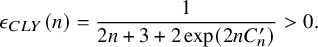 $$ \begin{align*}\epsilon_{CLY}(n)=\frac{1}{2n+3+2 \exp(2n C_n^{\prime})}>0. \end{align*} $$
Cheng–Li–Yau [Reference Cheng, Li and Yau15] show that if $\mathcal {C}\subset \mathbb {R}^{n+1}$
is a non-flat regular minimal cone, then
$\mathcal {C}\subset \mathbb {R}^{n+1}$
is a non-flat regular minimal cone, then
 $$ \begin{align*}\Theta(\mathcal{C})\geq 1+\epsilon_{CLY}(n). \end{align*} $$
These numbers are very small. Indeed, for $n\geq 3$
,
$n\geq 3$
,
 $$ \begin{align*}2.3\times 10^{-10}\approx \epsilon_{CLY}(3)> \epsilon_{CLY}(n). \end{align*} $$
Funding statement
The first author was partially supported by grants from the National Science Foundation (DMS-1904674 and DMS-2203132). The second author was partially supported by a grant from the National Science Foundation (DMS-2146997).
Competing interest
The authors have no competing interests to declare.


 Open access