


1 Introduction
1.1
The main objective of this paper is to construct regular integral models for some Shimura varieties over places of bad reduction. Results of this type have already been obtained by Rapoport-Zink [Reference Rapoport and Zink24], Pappas [Reference Pappas16] and He-Pappas-Rapoport [Reference He, Pappas and Rapoport12] in specific instances. Here, we consider Shimura varieties associated to unitary similitude groups of signature $(r,s)$
over an imaginary quadratic field K. These Shimura varieties are moduli spaces of abelian varieties with polarization, endomorphisms and level structure (Shimura varieties of PEL type). Shimura varieties have canonical models over the ‘reflex’ number field E, and in the cases we consider, the reflex field is the field of rational numbers
$(r,s)$
over an imaginary quadratic field K. These Shimura varieties are moduli spaces of abelian varieties with polarization, endomorphisms and level structure (Shimura varieties of PEL type). Shimura varieties have canonical models over the ‘reflex’ number field E, and in the cases we consider, the reflex field is the field of rational numbers $\mathbb {Q}$
if
$\mathbb {Q}$
if $r = s$
and
$r = s$
and $E = K$
otherwise [Reference Pappas15, §3].
$E = K$
otherwise [Reference Pappas15, §3].
Constructing such well-behaved integral models is an interesting and challenging problem, with several applications to number theory. The behavior of these depends very much on the ‘level subgroup’. Here, the level subgroup is the stabilizer of a $\pi $
-modular lattice in the hermitian space. (This is a lattice which is equal to its dual times a uniformizer). For this level subgroup, and the signatures
$\pi $
-modular lattice in the hermitian space. (This is a lattice which is equal to its dual times a uniformizer). For this level subgroup, and the signatures $(n-s,s)$
with n even and
$(n-s,s)$
with n even and $s \leq 3$
, we show that there is a good (semi-stable) model.
$s \leq 3$
, we show that there is a good (semi-stable) model.
By using work of Rapoport-Zink [Reference Rapoport and Zink24] and Pappas [Reference Pappas15], we first construct p-adic integral models, which have simple and explicit moduli descriptions but are not always flat. These models are étale locally around each point isomorphic to certain simpler schemes the naive local models. Inspired by the work of Pappas-Rapoport [Reference Pappas and Rapoport17] and Krämer [Reference Krämer14], we consider a variation of the above moduli problem where we add in the moduli problem an additional subspace in the deRham filtration $ \mathrm {Fil}^0 (A) \subset H_{dR}^1(A)$
of the universal abelian variety A, which satisfies certain conditions. This is essentially an instance of the notion of a ‘linear modification’ introduced in [Reference Pappas15]. Then for the signatures
$ \mathrm {Fil}^0 (A) \subset H_{dR}^1(A)$
of the universal abelian variety A, which satisfies certain conditions. This is essentially an instance of the notion of a ‘linear modification’ introduced in [Reference Pappas15]. Then for the signatures $(n-s,s)$
, with
$(n-s,s)$
, with $s \leq 3$
, we calculate the flat closure of these models, and we show that they are smooth when
$s \leq 3$
, we calculate the flat closure of these models, and we show that they are smooth when $s=1$
and have semi-stable reduction when
$s=1$
and have semi-stable reduction when $s=2$
or
$s=2$
or $s=3$
(i.e., they are regular and the irreducible components of the special fiber are smooth divisors crossing normally). Moreover, we want to mention that we obtain a moduli description of this flat closure. We anticipate that our construction will have applications to the study of arithmetic intersections of special cycles and Kudla’s program. (See, for example, [Reference Zhang29], [Reference Bruinier, Howard, Kudla, Rapoport and Yang6] and [Reference He, Li, Shi and Yang11], for some works in this direction.)
$s=3$
(i.e., they are regular and the irreducible components of the special fiber are smooth divisors crossing normally). Moreover, we want to mention that we obtain a moduli description of this flat closure. We anticipate that our construction will have applications to the study of arithmetic intersections of special cycles and Kudla’s program. (See, for example, [Reference Zhang29], [Reference Bruinier, Howard, Kudla, Rapoport and Yang6] and [Reference He, Li, Shi and Yang11], for some works in this direction.)
1.2
Let us introduce some notation first. Recall that K is an imaginary quadratic field and we fix an embedding $\varepsilon : K\rightarrow \mathbb {C}$
. Let W be a n-dimensional K-vector space, equipped with a nondegenerate hermitian form
$\varepsilon : K\rightarrow \mathbb {C}$
. Let W be a n-dimensional K-vector space, equipped with a nondegenerate hermitian form $\phi $
. Consider the group
$\phi $
. Consider the group $G = \mathrm {GU}_n$
of unitary similitudes for
$G = \mathrm {GU}_n$
of unitary similitudes for $(W,\phi )$
of dimension
$(W,\phi )$
of dimension $n\geq 3$
over K. We fix a conjugacy class of homomorphisms
$n\geq 3$
over K. We fix a conjugacy class of homomorphisms $h: \mathrm {Res}_{\mathbb {C}/\mathbb {R}}\mathbb {G}_{m,\mathbb {C}}\rightarrow \mathrm {GU}_n$
corresponding to a Shimura datum
$h: \mathrm {Res}_{\mathbb {C}/\mathbb {R}}\mathbb {G}_{m,\mathbb {C}}\rightarrow \mathrm {GU}_n$
corresponding to a Shimura datum $(G,X_h)$
of signature
$(G,X_h)$
of signature $(r,s)$
. Set
$(r,s)$
. Set $X = X_h$
. The pair
$X = X_h$
. The pair $(G,X)$
gives rise to a Shimura variety
$(G,X)$
gives rise to a Shimura variety $Sh(G,X)$
over the reflex field E (see [Reference Pappas and Rapoport18, §1.1] for more details). Let p be an odd prime number which ramifies in K. Set
$Sh(G,X)$
over the reflex field E (see [Reference Pappas and Rapoport18, §1.1] for more details). Let p be an odd prime number which ramifies in K. Set $K_1=K\otimes _{\mathbb {Q}} \mathbb {Q}_p$
with a uniformizer
$K_1=K\otimes _{\mathbb {Q}} \mathbb {Q}_p$
with a uniformizer $\pi $
, and
$\pi $
, and $V=W\otimes _{\mathbb {Q}} \mathbb {Q}_p$
. We assume that the hermitian form
$V=W\otimes _{\mathbb {Q}} \mathbb {Q}_p$
. We assume that the hermitian form $\phi $
is split on V (i.e., there is a basis
$\phi $
is split on V (i.e., there is a basis $e_1, \dots , e_n$
such that
$e_1, \dots , e_n$
such that $\phi (e_i, e_{n+1-j})=\delta _{ij}$
for
$\phi (e_i, e_{n+1-j})=\delta _{ij}$
for $1\leq i, j\leq n$
). We denote by
$1\leq i, j\leq n$
). We denote by
 $$\begin{align*}\Lambda_i = \text{span}_{O_{K_1}} \{\pi^{-1}e_1, \dots, \pi^{-1}e_i, e_{i+1}, \dots, e_n\} \end{align*}$$
the standard lattices in V. We can complete this into a self dual lattice chain by setting $\Lambda _{i+kn}:=\pi ^{-k}\Lambda _i$
(see §2.1).
$\Lambda _{i+kn}:=\pi ^{-k}\Lambda _i$
(see §2.1).
By [Reference Pappas and Rapoport18], there are 3 different types of the special maximal parahoric subgroups of $\mathrm {GU}_n$
depending on the parity of n. More precisely, consider the stabilizer subgroup
$\mathrm {GU}_n$
depending on the parity of n. More precisely, consider the stabilizer subgroup
 $$\begin{align*}P_I:=\{g\in\mathrm{GU}_n\mid g\Lambda_i=\Lambda_i , \quad \forall i \in I\}, \end{align*}$$
where I is a nonempty subset of $\{0,\dots , \lfloor n/2\rfloor \}$
. When
$\{0,\dots , \lfloor n/2\rfloor \}$
. When $n=2m+1$
is odd, the special maximal parahoric subgroups are conjugate to the stabilizer subgroup
$n=2m+1$
is odd, the special maximal parahoric subgroups are conjugate to the stabilizer subgroup $P_{\{0\}}$
or
$P_{\{0\}}$
or $P_{\{m\}}$
. When
$P_{\{m\}}$
. When $n=2m$
is even, the special maximal parahoric subgroups are conjugate to the stabilizer subgroup
$n=2m$
is even, the special maximal parahoric subgroups are conjugate to the stabilizer subgroup $P_{\{m\}}$
. In this article, we consider the special maximal parahoric subgroup
$P_{\{m\}}$
. In this article, we consider the special maximal parahoric subgroup $P_{\{m\}}$
when
$P_{\{m\}}$
when $n=2m$
is even. We intend to take up the case
$n=2m$
is even. We intend to take up the case $n=2m+1, I=\{m\}$
in a subsequent work.
$n=2m+1, I=\{m\}$
in a subsequent work.
To explain our results, we assume $n=2m$
, and
$n=2m$
, and $(r,s)=(n-1,1)$
or
$(r,s)=(n-1,1)$
or $(n-2,2)$
or
$(n-2,2)$
or $(n-3,3)$
. Denote by
$(n-3,3)$
. Denote by $P_{\{m\}}$
the stabilizer of
$P_{\{m\}}$
the stabilizer of $\Lambda _m$
in
$\Lambda _m$
in $G(\mathbb {Q}_p)$
. We let
$G(\mathbb {Q}_p)$
. We let $\mathcal {L}$
be the self-dual multichain consisting of lattices
$\mathcal {L}$
be the self-dual multichain consisting of lattices $\{\Lambda _j\}_{j\in n\mathbb {Z} \pm m}$
. Here,
$\{\Lambda _j\}_{j\in n\mathbb {Z} \pm m}$
. Here, $\mathcal {G} = \underline {\mathrm {Aut}}(\mathcal {L})$
is the (smooth) group scheme over
$\mathcal {G} = \underline {\mathrm {Aut}}(\mathcal {L})$
is the (smooth) group scheme over $\mathbb {Z}_p$
with
$\mathbb {Z}_p$
with $P_{\{m\}} = \mathcal {G}(\mathbb {Z}_p)$
the subgroup of
$P_{\{m\}} = \mathcal {G}(\mathbb {Z}_p)$
the subgroup of $G(\mathbb {Q}_p)$
fixing the lattice chain
$G(\mathbb {Q}_p)$
fixing the lattice chain $\mathcal {L}$
.
$\mathcal {L}$
.
Choose also a sufficiently small compact open subgroup $K^p$
of the prime-to-p finite adelic points
$K^p$
of the prime-to-p finite adelic points $G({\mathbb A}_{f}^p)$
of G and set
$G({\mathbb A}_{f}^p)$
of G and set $\mathbf {K}=K^pP_{\{m\}}$
. The Shimura variety
$\mathbf {K}=K^pP_{\{m\}}$
. The Shimura variety $\mathrm { Sh}_{\mathbf {K}}(G, X)$
with complex points
$\mathrm { Sh}_{\mathbf {K}}(G, X)$
with complex points
 $$\begin{align*}\mathrm{Sh}_{\mathbf{K}}(G, X)(\mathbb{C})=G(\mathbb{Q})\backslash X\times G({\mathbb A}_{f})/\mathbf{K} \end{align*}$$
is of PEL type and has a canonical model over the reflex field E. We set $\mathcal {O} = O_{E_v}$
, where v the unique prime ideal of E above
$\mathcal {O} = O_{E_v}$
, where v the unique prime ideal of E above $(p)$
.
$(p)$
.
We consider the moduli functor $\mathcal {A}^{\mathrm {naive}}_{\mathbf {K}}$
over
$\mathcal {A}^{\mathrm {naive}}_{\mathbf {K}}$
over $\mathrm {Spec \, } \mathcal {O} $
given in [Reference Rapoport and Zink24, Definition 6.9]:
$\mathrm {Spec \, } \mathcal {O} $
given in [Reference Rapoport and Zink24, Definition 6.9]:
A point of $\mathcal {A}^{\mathrm {naive}}_{\mathbf {K}}$
with values in the
$\mathcal {A}^{\mathrm {naive}}_{\mathbf {K}}$
with values in the $\mathcal {O} $
-scheme S is the isomorphism class of the following set of data
$\mathcal {O} $
-scheme S is the isomorphism class of the following set of data $(A,\iota ,\bar {\lambda }, \bar {\eta })$
:
$(A,\iota ,\bar {\lambda }, \bar {\eta })$
:
-
(1) An object $(A,\iota )$
, where A is an abelian scheme with relative dimension n over S (terminology of [Reference Rapoport and Zink24]), compatibly endowed with an action of
${\mathcal O}$
:
$$\begin{align*}\iota: {\mathcal O} \rightarrow \text{End} \,A \otimes \mathbb{Z}_p.\end{align*}$$
$(A,\iota )$
, where A is an abelian scheme with relative dimension n over S (terminology of [Reference Rapoport and Zink24]), compatibly endowed with an action of
${\mathcal O}$
:
$$\begin{align*}\iota: {\mathcal O} \rightarrow \text{End} \,A \otimes \mathbb{Z}_p.\end{align*}$$
-
(2) A
$\mathbb {Q}$
-homogeneous principal polarization
$\bar {\lambda }$
of the
$\mathcal {L}$
-set A. -
(3) A
$K^p$
-level structure which respects the bilinear forms on both sides up to a constant in
$$\begin{align*}\bar{\eta} : H_1 (A, {\mathbb A}_{f}^p) \simeq W \otimes {\mathbb A}_{f}^p \, \text{ mod} \, K^p \end{align*}$$
$({\mathbb A}_{f}^p)^{\times }$
(see loc. cit. for details). The set A should satisfy the determinant condition (i) of loc. cit. which depends on
$(r,s)$
.


For the definitions of the terms employed here, we refer to loc.cit., 6.3–6.8 and [Reference Pappas15, §3]. The functor $\mathcal {A}^{\mathrm {naive}}_{\mathbf {K}}$
is representable by a quasi-projective scheme over
$\mathcal {A}^{\mathrm {naive}}_{\mathbf {K}}$
is representable by a quasi-projective scheme over $\mathcal {O}$
. Since the Hasse principle is satisfied for the unitary group, we can see as in loc. cit. that there is a natural isomorphism
$\mathcal {O}$
. Since the Hasse principle is satisfied for the unitary group, we can see as in loc. cit. that there is a natural isomorphism
 $$\begin{align*}\mathcal{A}^{\mathrm{naive}}_{\mathbf{K}} \otimes_{{\mathcal O}} E_v = \mathrm{Sh}_{\mathbf{K}}(G, X)\otimes_{E} E_v. \end{align*}$$
The moduli scheme $\mathcal {A}^{\mathrm {naive}}_{\mathbf {K}}$
is connected to the naive local model
$\mathcal {A}^{\mathrm {naive}}_{\mathbf {K}}$
is connected to the naive local model $\mathrm {M}^{\mathrm {naive}}$
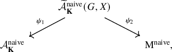
(see §3 for the explicit definition). As is explained in [Reference Rapoport and Zink24] and [Reference Pappas15], the naive local model is connected to the moduli scheme
$\mathrm {M}^{\mathrm {naive}}$
(see §3 for the explicit definition). As is explained in [Reference Rapoport and Zink24] and [Reference Pappas15], the naive local model is connected to the moduli scheme $\mathcal {A}^{\mathrm {naive}}_{\mathbf {K}}$
via the local model diagram
$\mathcal {A}^{\mathrm {naive}}_{\mathbf {K}}$
via the local model diagram
where the morphism $\psi _1$
is a
$\psi _1$
is a $\mathcal {G}$
-torsor and
$\mathcal {G}$
-torsor and $\psi _2$
is a smooth and
$\psi _2$
is a smooth and $\mathcal {G}$
-equivariant morphism. In particular, since
$\mathcal {G}$
-equivariant morphism. In particular, since ${\mathcal G}$
is smooth, the above imply that
${\mathcal G}$
is smooth, the above imply that $\mathcal {A}^{\mathrm {naive}}_{\mathbf {K}} $
is étale locally isomorphic to
$\mathcal {A}^{\mathrm {naive}}_{\mathbf {K}} $
is étale locally isomorphic to $\mathrm {M}^{\mathrm {naive}}$
. From [Reference Pappas, Rapoport and Smithling20, Remark 2.6.10], we have that the naive local model is never flat, and by the above, the same is true for
$\mathrm {M}^{\mathrm {naive}}$
. From [Reference Pappas, Rapoport and Smithling20, Remark 2.6.10], we have that the naive local model is never flat, and by the above, the same is true for $\mathcal {A}^{\mathrm {naive}}_{\mathbf {K}} $
. Denote by
$\mathcal {A}^{\mathrm {naive}}_{\mathbf {K}} $
. Denote by $ \mathcal {A}^{\mathrm {flat}}_{\mathbf {K}} $
the flat closure of
$ \mathcal {A}^{\mathrm {flat}}_{\mathbf {K}} $
the flat closure of $\mathrm {Sh}_{\mathbf {K}}(G, X)\otimes _{E} E_v$
in
$\mathrm {Sh}_{\mathbf {K}}(G, X)\otimes _{E} E_v$
in $ \mathcal {A}^{\mathrm {naive}}_{\mathbf {K}}$
. As in [Reference Pappas and Rapoport18], there is a relatively representable smooth morphism of relative dimension
$ \mathcal {A}^{\mathrm {naive}}_{\mathbf {K}}$
. As in [Reference Pappas and Rapoport18], there is a relatively representable smooth morphism of relative dimension $\mathrm {dim} (G)$
,
$\mathrm {dim} (G)$
,
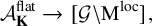 $$\begin{align*}\mathcal{A}^{\mathrm{flat}}_{\mathbf{K}} \to [\mathcal{G} \backslash \mathrm{M}^{\mathrm{loc}}], \end{align*}$$
where the local model $\mathrm {M}^{\mathrm {loc}} $
is defined as the flat closure of
$\mathrm {M}^{\mathrm {loc}} $
is defined as the flat closure of $ \mathrm {M}^{\mathrm {naive}} \otimes _{\mathcal {O}} E_v$
in
$ \mathrm {M}^{\mathrm {naive}} \otimes _{\mathcal {O}} E_v$
in $\mathrm {M}^{\mathrm {naive}}$
. This of course implies that
$\mathrm {M}^{\mathrm {naive}}$
. This of course implies that $\mathcal {A}^{\mathrm {flat}}_{\mathbf {K}}$
is étale locally isomorphic to the local model
$\mathcal {A}^{\mathrm {flat}}_{\mathbf {K}}$
is étale locally isomorphic to the local model $\mathrm {M}^{\mathrm {loc}}$
.
$\mathrm {M}^{\mathrm {loc}}$
.
We now consider a variation of the moduli of abelian schemes $\mathcal {A}_{\mathbf {K}}$
where we add in the moduli problem an additional subspace in the Hodge filtration
$\mathcal {A}_{\mathbf {K}}$
where we add in the moduli problem an additional subspace in the Hodge filtration $ \mathrm {Fil}^0 (A) \subset H_{dR}^1(A)$
of the universal abelian variety A (see [Reference Haines7, §6.3] for more details) with certain conditions to imitate the definition of the naive splitting model
$ \mathrm {Fil}^0 (A) \subset H_{dR}^1(A)$
of the universal abelian variety A (see [Reference Haines7, §6.3] for more details) with certain conditions to imitate the definition of the naive splitting model $\mathcal {M}$
(we refer to §3 for the explicit definition). There is a projective forgetful morphism
$\mathcal {M}$
(we refer to §3 for the explicit definition). There is a projective forgetful morphism
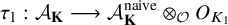 $$\begin{align*}\tau_1 : \mathcal{A}_{\mathbf{K}} \longrightarrow \mathcal{A}^{\mathrm{naive}}_{\mathbf{K}}\otimes_{\mathcal{O}} O_{K_1}\end{align*}$$
which induces an isomorphism over the generic fibers (see §6). Moreover, $\mathcal {A}_{\mathbf {K}}$
has the same étale local structure as
$\mathcal {A}_{\mathbf {K}}$
has the same étale local structure as $\mathcal {M}$
; it is a ‘linear modification’ of
$\mathcal {M}$
; it is a ‘linear modification’ of $\mathcal {A}^{\mathrm {naive}}_{\mathbf {K}}\otimes _{\mathcal {O}} O_{K_1}$
in the sense of [Reference Pappas15, §2] (see also [Reference Pappas and Rapoport17, §15]). Note that there is also a corresponding projective forgetful morphism
$\mathcal {A}^{\mathrm {naive}}_{\mathbf {K}}\otimes _{\mathcal {O}} O_{K_1}$
in the sense of [Reference Pappas15, §2] (see also [Reference Pappas and Rapoport17, §15]). Note that there is also a corresponding projective forgetful morphism
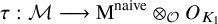 $$\begin{align*}\tau : \mathcal{M} \longrightarrow \mathrm{M}^{\mathrm{naive}} \otimes_{\mathcal{O}} O_{K_1} \end{align*}$$
which induces an isomorphism over the generic fibers (see §3). In §5, we show that $\mathcal {M}$
is not flat for any signature
$\mathcal {M}$
is not flat for any signature $(r,s)$
, and the same is true for
$(r,s)$
, and the same is true for $ \mathcal {A}_{\mathbf {K}}$
. In fact,
$ \mathcal {A}_{\mathbf {K}}$
. In fact, $\mathcal {M}$
is not topologically flat since there exists a point which cannot lift to characteristic zero (see Proposition 5.1). This type of phenomenon is similar to what already has been observed for this level subgroup for the wedge local models in [Reference Pappas and Rapoport18, Remark 5.3] (see §3 for the definition of wedge local models). Consider the closed subscheme
$\mathcal {M}$
is not topologically flat since there exists a point which cannot lift to characteristic zero (see Proposition 5.1). This type of phenomenon is similar to what already has been observed for this level subgroup for the wedge local models in [Reference Pappas and Rapoport18, Remark 5.3] (see §3 for the definition of wedge local models). Consider the closed subscheme $\mathcal {A}^{\mathrm {spl}}_{\mathbf {K}} \subset \mathcal {A}_{\mathbf {K}} $
defined as
$\mathcal {A}^{\mathrm {spl}}_{\mathbf {K}} \subset \mathcal {A}_{\mathbf {K}} $
defined as $\mathcal {A}^{\mathrm {spl}}_{\mathbf {K}} :=\tau _1^{-1} (\mathcal {A}^{\mathrm {flat}}_{\mathbf {K}}) $
. It is a linear modification of
$\mathcal {A}^{\mathrm {spl}}_{\mathbf {K}} :=\tau _1^{-1} (\mathcal {A}^{\mathrm {flat}}_{\mathbf {K}}) $
. It is a linear modification of $\mathcal {A}^{\mathrm {naive}}_{\mathbf {K}}\otimes _{\mathcal {O}} O_{K_1}$
.
$\mathcal {A}^{\mathrm {naive}}_{\mathbf {K}}\otimes _{\mathcal {O}} O_{K_1}$
.
1.3
One of the main results of the present paper is the following theorem.
Theorem 1.1. Assume that $ (r,s) = (n-1,1)$
or
$ (r,s) = (n-1,1)$
or $(n-2,2)$
or
$(n-2,2)$
or $(n-3,3)$
. For every
$(n-3,3)$
. For every $K^p$
as above, there is a scheme
$K^p$
as above, there is a scheme $\mathcal {A}^{\mathrm {spl}}_{\mathbf {K}}$
, flat over
$\mathcal {A}^{\mathrm {spl}}_{\mathbf {K}}$
, flat over $\mathrm {Spec \, } (O_{K_1})$
, with
$\mathrm {Spec \, } (O_{K_1})$
, with
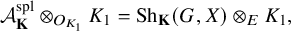 $$\begin{align*}\mathcal{A}^{\mathrm{spl}}_{\mathbf{K}}\otimes_{O_{K_1}} K_1=\mathrm{Sh}_{\mathbf{K}}(G, X)\otimes_{E} K_1, \end{align*}$$
and which supports a local model diagram
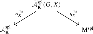
such that:
-
a)
$\pi ^{\mathrm {reg}}_{\mathbf {K}}$
is a
$\mathcal {G}$
-torsor for the parahoric group scheme
${\mathcal G}$
that corresponds to
$P_{\{m\}}$
. -
b)
$q^{\mathrm {reg}}_{\mathbf {K}}$
is smooth and
${\mathcal G}$
-equivariant. -
c) When
$(r,s) = (n-1,1)$
,
$\mathcal {A}^{\mathrm {spl}}_{\mathbf {K}}$
is a smooth scheme. -
c’) When
$(r,s) = (n-2,2)$
or
$(r,s) =(n-3,3)$
,
$\mathcal {A}^{\mathrm {spl}}_{\mathbf {K}}$
has semi-stable reduction. In particular,
$\mathcal {A}^{\mathrm {spl}}_{\mathbf {K}}$
is regular and has special fiber which is a reduced divisor with normal crossings.


In the above, the splitting model $\mathrm {M}^{\mathrm {spl}}$
is defined as
$\mathrm {M}^{\mathrm {spl}}$
is defined as $ \mathrm {M}^{\mathrm {spl}}:=\tau ^{-1}(\mathrm {M}^{\mathrm {loc}})$
. Since every point of
$ \mathrm {M}^{\mathrm {spl}}:=\tau ^{-1}(\mathrm {M}^{\mathrm {loc}})$
. Since every point of $\mathcal {A}^{\mathrm {spl}}_{\mathbf {K}} $
has an étale neighborhood which is also étale over
$\mathcal {A}^{\mathrm {spl}}_{\mathbf {K}} $
has an étale neighborhood which is also étale over $\mathrm {M}^{\mathrm {spl}}$
, it is enough to show that
$\mathrm {M}^{\mathrm {spl}}$
, it is enough to show that $\mathrm {M}^{\mathrm {spl}}$
has the above nice properties. To show this, we explicitly calculate an affine chart
$\mathrm {M}^{\mathrm {spl}}$
has the above nice properties. To show this, we explicitly calculate an affine chart $\mathcal {U}$
of
$\mathcal {U}$
of $\mathrm {M}^{\mathrm {spl}}$
in a neighbourhood of
$\mathrm {M}^{\mathrm {spl}}$
in a neighbourhood of $ \tau ^{-1}(*)$
, where
$ \tau ^{-1}(*)$
, where $*$
is a point from the unique closed
$*$
is a point from the unique closed $\mathcal {G}$
-orbit supported in the special fiber of
$\mathcal {G}$
-orbit supported in the special fiber of $\mathrm {M}^{\mathrm {loc}}$
(see [Reference Pappas15, §4] for more details). Note that the unique closed
$\mathrm {M}^{\mathrm {loc}}$
(see [Reference Pappas15, §4] for more details). Note that the unique closed $\mathcal {G}$
-orbit depends on the parity of s (see §3). We treat these two cases (i.e., when s is even and odd) separately in §4.1 and §4.2.
$\mathcal {G}$
-orbit depends on the parity of s (see §3). We treat these two cases (i.e., when s is even and odd) separately in §4.1 and §4.2.
Moreover, we give a moduli-theoretic description of $\mathrm {M}^{\mathrm {spl}}$
and so by the above for
$\mathrm {M}^{\mathrm {spl}}$
and so by the above for $\mathcal {A}^{\mathrm {spl}}_{\mathbf {K}}$
. Inspired by the work of Pappas-Rapoport [Reference Pappas and Rapoport18], we define the closed subscheme
$\mathcal {A}^{\mathrm {spl}}_{\mathbf {K}}$
. Inspired by the work of Pappas-Rapoport [Reference Pappas and Rapoport18], we define the closed subscheme $ \mathcal {M}^{\mathrm {spin}} \subset \mathcal {M}$
by adding the ‘spin condition’ (see §7) and we show the following.
$ \mathcal {M}^{\mathrm {spin}} \subset \mathcal {M}$
by adding the ‘spin condition’ (see §7) and we show the following.
Theorem 1.2. For the signatures $(n-s,s)$
with
$(n-s,s)$
with $s\leq 3$
, we have
$s\leq 3$
, we have $ \mathcal {M}^{\mathrm {spin}}=\mathrm {M}^{\mathrm {spl}}$
.
$ \mathcal {M}^{\mathrm {spin}}=\mathrm {M}^{\mathrm {spl}}$
.
Here, we note that at the level of local models, a moduli description of $\mathrm {M}^{\mathrm {loc}}$
for the signature
$\mathrm {M}^{\mathrm {loc}}$
for the signature $(n-1,1)$
can be obtained by adding the ‘wedge and spin condition’ to the moduli problem of
$(n-1,1)$
can be obtained by adding the ‘wedge and spin condition’ to the moduli problem of $\mathrm {M}^{\mathrm {naive}}$
(see [Reference Rapoport, Smithling and Zhang22]). For higher signatures, it has been conjectured that we can get the moduli description of
$\mathrm {M}^{\mathrm {naive}}$
(see [Reference Rapoport, Smithling and Zhang22]). For higher signatures, it has been conjectured that we can get the moduli description of $\mathrm {M}^{\mathrm {loc}}$
by adding the ‘wedge and spin conditions’ to
$\mathrm {M}^{\mathrm {loc}}$
by adding the ‘wedge and spin conditions’ to $\mathrm {M}^{\mathrm {naive}}$
; see the survey paper [Reference Pappas, Rapoport and Smithling20] for more details.
$\mathrm {M}^{\mathrm {naive}}$
; see the survey paper [Reference Pappas, Rapoport and Smithling20] for more details.
Before we move on to the description of $\mathcal {U}$
, we want to give a brief historical outline about the splitting models. Splitting models were first described for associated Shimura varieties of type A and type C by Pappas-Rapoport [Reference Pappas and Rapoport17]. For unitary groups, Krämer [Reference Krämer14] first showed that the splitting model has semi-stable reduction for the signature
$\mathcal {U}$
, we want to give a brief historical outline about the splitting models. Splitting models were first described for associated Shimura varieties of type A and type C by Pappas-Rapoport [Reference Pappas and Rapoport17]. For unitary groups, Krämer [Reference Krämer14] first showed that the splitting model has semi-stable reduction for the signature $(r,s)=(n-1,1)$
when
$(r,s)=(n-1,1)$
when $n=2m+1, I=\{0\}$
. When the signature is
$n=2m+1, I=\{0\}$
. When the signature is $(r,s)=(n-2,2)$
, the first author [Reference Zachos28] showed that the corresponding splitting model
$(r,s)=(n-2,2)$
, the first author [Reference Zachos28] showed that the corresponding splitting model $\mathcal {M}$
does not have semi-stable reduction. Then, he resolved the singularities by giving an explicit blow-up of
$\mathcal {M}$
does not have semi-stable reduction. Then, he resolved the singularities by giving an explicit blow-up of $\mathcal {M}$
along a smooth divisor. For more information on the geometry of the special fiber of
$\mathcal {M}$
along a smooth divisor. For more information on the geometry of the special fiber of $\mathcal {M}$
for general signature
$\mathcal {M}$
for general signature $(r,s)$
, we refer the reader to the very recent work of Bijakowski and Hernandez [Reference Bijakowski and Hernandez4]. Lastly, we want to mention the work of the second author where he considered the splitting model for triality groups in [Reference Zhao30] (see also [Reference Zhao31]).
$(r,s)$
, we refer the reader to the very recent work of Bijakowski and Hernandez [Reference Bijakowski and Hernandez4]. Lastly, we want to mention the work of the second author where he considered the splitting model for triality groups in [Reference Zhao30] (see also [Reference Zhao31]).
For the rest of this subsection, we fix $n=2m$
and
$n=2m$
and $I=\{m\}$
. Define
$I=\{m\}$
. Define
 $$\begin{align*}J_n = \left[\begin{array}{@{}c|c@{}}0_m & -H_m \\ H_m & 0_m\end{array}\right], \end{align*}$$
where $H_m$
is the unit antidiagonal matrix (of size m). For a general signature
$H_m$
is the unit antidiagonal matrix (of size m). For a general signature $(r,s)$
, we first obtain the following:
$(r,s)$
, we first obtain the following:
Theorem 1.3.
(1) When s is even, there is an affine chart $\mathcal {U} \subset \mathcal {M}$
which is isomorphic to
$\mathcal {U} \subset \mathcal {M}$
which is isomorphic to $\mathrm {Spec \, } O_{K_1}[X,Y]/I $
, where
$\mathrm {Spec \, } O_{K_1}[X,Y]/I $
, where
 $$\begin{align*}I = \left(Y'-I_s, \,\, X+X^t, \,\, X\cdot Y^t \cdot J_n \cdot Y +2 \pi I_s\right) \end{align*}$$
for some choice of $Y'$
. Here, X, Y are matrices of sizes
$Y'$
. Here, X, Y are matrices of sizes $s\times s$
and
$s\times s$
and $n\times s$
, respectively, with indeterminates as entries and
$n\times s$
, respectively, with indeterminates as entries and $Y'$
is a submatrix of Y of size
$Y'$
is a submatrix of Y of size $ s \times s$
(i.e., it is composed of s rows from Y along with the corresponding s columns).
$ s \times s$
(i.e., it is composed of s rows from Y along with the corresponding s columns).
(2a) When $s=1$
, there is an affine chart
$s=1$
, there is an affine chart $\mathcal {U} \subset \mathcal {M}$
which is isomorphic to
$\mathcal {U} \subset \mathcal {M}$
which is isomorphic to $\mathbb {A}_{O_{K_1}}^{n-1}$
.
$\mathbb {A}_{O_{K_1}}^{n-1}$
.
(2b) When s is odd and $s\geq 3$
, there is an affine chart
$s\geq 3$
, there is an affine chart $\mathcal {U} \subset \mathcal {M}$
which is isomorphic to
$\mathcal {U} \subset \mathcal {M}$
which is isomorphic to $\mathbb {A}_{O_{K_1}}^{s-1}\times \mathrm {Spec \, } O_{K_1}[X, Y]/I$
, where
$\mathbb {A}_{O_{K_1}}^{s-1}\times \mathrm {Spec \, } O_{K_1}[X, Y]/I$
, where
 $$\begin{align*}I=(Y'-[\mathbf{0}\mid I_{s-1}], \,\, X+X^t, \,\, X\cdot Y^t \cdot J_{n-2} \cdot Y +2\pi I_{s-1}) \end{align*}$$
for some choice of $Y'$
. Here, X, Y are matrices of sizes
$Y'$
. Here, X, Y are matrices of sizes $(s-1)\times (s-1)$
and
$(s-1)\times (s-1)$
and $(n-2)\times s$
, respectively, with indeterminates as entries and
$(n-2)\times s$
, respectively, with indeterminates as entries and $Y'$
is a submatrix of Y of size
$Y'$
is a submatrix of Y of size $ (s-1)\times s$
(i.e., it is composed of
$ (s-1)\times s$
(i.e., it is composed of $(s-1)$
rows from Y along with the corresponding s columns).
$(s-1)$
rows from Y along with the corresponding s columns).
By using the explicit description of $\mathcal {U}$
above, we prove that
$\mathcal {U}$
above, we prove that $\mathcal {G}$
-translates of
$\mathcal {G}$
-translates of $\mathcal {U}$
cover
$\mathcal {U}$
cover $\mathrm {M}^{\mathrm {spl}}$
and we deduce the following:
$\mathrm {M}^{\mathrm {spl}}$
and we deduce the following:
Theorem 1.4.
-
a) When
$s=1$
,
$\mathrm {M}^{\mathrm {spl}}$
is a smooth scheme. -
b) When
$s=2$
or
$s=3$
,
$\mathrm {M}^{\mathrm {spl}}$
has semi-stable reduction. In particular,
$\mathrm {M}^{\mathrm {spl}}$
is regular and has special fiber a reduced divisor with two smooth irreducible components intersecting transversely.


When $s=2$
or
$s=2$
or $s=3$
, we show, by using Theorem 1.2, that one of the two components of the special fiber of
$s=3$
, we show, by using Theorem 1.2, that one of the two components of the special fiber of $\mathrm {M}^{\mathrm {spl}}$
maps birationally to the special fiber of
$\mathrm {M}^{\mathrm {spl}}$
maps birationally to the special fiber of $\mathrm { M}^{\mathrm {loc}}$
while the other irreducible component is the inverse image of the unique closed
$\mathrm { M}^{\mathrm {loc}}$
while the other irreducible component is the inverse image of the unique closed ${\mathcal G}$
-orbit.
${\mathcal G}$
-orbit.
Moreover, for $(r,s)=(n-1,1) $
, we deduce that
$(r,s)=(n-1,1) $
, we deduce that $ \mathrm {M}^{\mathrm {spl}}$
is equal to the local model
$ \mathrm {M}^{\mathrm {spl}}$
is equal to the local model $\mathrm {M}^{\mathrm {loc}} \otimes _{\mathcal {O}} O_{K_1}$
(see Remark 5.12). In [Reference Pappas and Rapoport18, §5.3], the authors showed that
$\mathrm {M}^{\mathrm {loc}} \otimes _{\mathcal {O}} O_{K_1}$
(see Remark 5.12). In [Reference Pappas and Rapoport18, §5.3], the authors showed that $\mathrm {M}^{\mathrm {loc}}$
is smooth. This is a case of ‘exotic’ good reduction. We also refer the reader to the result of [Reference Haines and Richarz8] where the authors give an alternative explanation for the smoothness of
$\mathrm {M}^{\mathrm {loc}}$
is smooth. This is a case of ‘exotic’ good reduction. We also refer the reader to the result of [Reference Haines and Richarz8] where the authors give an alternative explanation for the smoothness of $\mathrm {M}^{\mathrm {loc}}$
by identifying its special fiber with a Schubert variety attached to a minuscule cocharacter in the twisted affine Grassmannian corresponding to
$\mathrm {M}^{\mathrm {loc}}$
by identifying its special fiber with a Schubert variety attached to a minuscule cocharacter in the twisted affine Grassmannian corresponding to $P_{\{m\}}$
.
$P_{\{m\}}$
.
Lastly, we want to mention that we can apply these results to obtain regular (formal) models of the corresponding Rapoport-Zink spaces.
Let us now outline the contents of the paper: In §2, we recall the parahoric subgroups of the unitary similitude group when $n=2m$
. In §3, we recall the definition of certain variants of local models for ramified unitary groups. The explicit equations of
$n=2m$
. In §3, we recall the definition of certain variants of local models for ramified unitary groups. The explicit equations of $\mathcal {U}$
are given in §4. In §5.1, we show that the naive splitting model
$\mathcal {U}$
are given in §4. In §5.1, we show that the naive splitting model $\mathcal {M}$
is not flat and prove that
$\mathcal {M}$
is not flat and prove that ${\mathcal G}$
-translates of
${\mathcal G}$
-translates of $\mathcal {U}$
cover
$\mathcal {U}$
cover $\mathrm {M}^{\mathrm {spl}}$
for the signature
$\mathrm {M}^{\mathrm {spl}}$
for the signature $(r,s)$
(
$(r,s)$
( $s\leq 3$
) in §5.2 and §5.3, respectively. In §6, we use the above results to construct smooth integral models for the signature
$s\leq 3$
) in §5.2 and §5.3, respectively. In §6, we use the above results to construct smooth integral models for the signature $(r,s)=(n-1,1)$
, and integral models with semi-stable reduction for
$(r,s)=(n-1,1)$
, and integral models with semi-stable reduction for $(r,s)=(n-2,2)$
and
$(r,s)=(n-2,2)$
and $(r,s)=(n-3,3)$
. In §7, we give a moduli-theoretic description of
$(r,s)=(n-3,3)$
. In §7, we give a moduli-theoretic description of $\mathrm {M}^{\mathrm {spl}}$
for
$\mathrm {M}^{\mathrm {spl}}$
for $s\leq 3$
by considering the spin condition.
$s\leq 3$
by considering the spin condition.
2 Preliminaries
2.1 Pairings and Standard Lattices
We use the notation of [Reference Pappas and Rapoport18]. Let $F_0$
be a complete discretely valued field with ring of integers
$F_0$
be a complete discretely valued field with ring of integers $O_{F_0}$
, perfect residue field k of characteristic
$O_{F_0}$
, perfect residue field k of characteristic $\neq 2$
, and uniformizer
$\neq 2$
, and uniformizer $\pi _0$
. Let
$\pi _0$
. Let $F/F_0$
be a ramified quadratic extension and
$F/F_0$
be a ramified quadratic extension and $\pi \in F$
a uniformizer with
$\pi \in F$
a uniformizer with $\pi ^2 = \pi _0$
. Let V be a F-vector space of dimension
$\pi ^2 = \pi _0$
. Let V be a F-vector space of dimension $n =2m> 3$
and let
$n =2m> 3$
and let
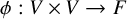 $$\begin{align*}\phi: V \times V \rightarrow F \end{align*}$$
be an $F/F_0$
-hermitian form. We assume that
$F/F_0$
-hermitian form. We assume that $\phi $
is split. This means that there exists a basis
$\phi $
is split. This means that there exists a basis $e_1, \dots , e_n$
of V such that
$e_1, \dots , e_n$
of V such that
 $$\begin{align*}\phi(e_i,e_{n+1-j}) = \delta_{i,j} \quad \text{for all} \quad i,j = 1, \dots, n. \end{align*}$$
We attach to $\phi $
the respective alternating and symmetric
$\phi $
the respective alternating and symmetric $F_0$
-bilinear forms
$F_0$
-bilinear forms $V \times V \rightarrow F_0$
 $$\begin{align*}\langle x, y \rangle = \frac{1}{2}\text{Tr}_{F /F_0} (\pi^{-1}\phi(x, y)) \quad \text{and} \quad ( x, y ) = \frac{1}{2}\text{Tr}_{F /F_0} (\phi(x, y)). \end{align*}$$
For any $O_F$
-lattice
$O_F$
-lattice $\Lambda $
in V, we denote by
$\Lambda $
in V, we denote by
 $$\begin{align*}\hat{\Lambda} = \{v \in V | \langle v, \Lambda \rangle \subset O_{F_0} \} \end{align*}$$
the dual lattice with respect to the alternating form and by
 $$\begin{align*}\hat{\Lambda}^s = \{v \in V | ( v, \Lambda ) \subset O_{F_0} \} \end{align*}$$
the dual lattice with respect to the symmetric form. We have $ \hat {\Lambda }^s = \pi ^{-1}\hat {\Lambda }.$
Both
$ \hat {\Lambda }^s = \pi ^{-1}\hat {\Lambda }.$
Both $\hat {\Lambda }$
and
$\hat {\Lambda }$
and $\hat {\Lambda }^s$
are
$\hat {\Lambda }^s$
are $O_F$
-lattices in V, and the forms
$O_F$
-lattices in V, and the forms $\langle \, , \, \rangle $
and
$\langle \, , \, \rangle $
and $ (\, , \,) $
induce perfect
$ (\, , \,) $
induce perfect $O_{F_0}$
-bilinear pairings
$O_{F_0}$
-bilinear pairings
 $$ \begin{align} \Lambda \times \hat{\Lambda} \xrightarrow{\langle \, , \, \rangle } O_{F_0}, \quad \Lambda \times \hat{\Lambda}^s \xrightarrow{ (\, , \,)} O_{F_0} \end{align} $$
for all $\Lambda $
. Also, the uniformizing element
$\Lambda $
. Also, the uniformizing element $\pi $
induces a
$\pi $
induces a $O_{F_0}$
- linear mapping on
$O_{F_0}$
- linear mapping on $\Lambda $
which we denote by t.
$\Lambda $
which we denote by t.
For $i= 0, \dots , n- 1$
, we define the standard lattices
$i= 0, \dots , n- 1$
, we define the standard lattices
 $$\begin{align*}\Lambda_i = \text{span}_{O_F} \{\pi^{-1}e_1, \dots, \pi^{-1}e_i, e_{i+1}, \dots, e_n\}. \end{align*}$$
We consider nonempty subsets $I \subset \{0, \dots , m\}$
with the property
$I \subset \{0, \dots , m\}$
with the property
 $$ \begin{align} m-1 \in I \Longrightarrow m \in I \end{align} $$
(see [Reference Pappas and Rapoport18, §1.2.3(b)] for more details). We complete the $\Lambda _i$
with
$\Lambda _i$
with $i \in I$
to a self-dual periodic lattice chain by first including the duals
$i \in I$
to a self-dual periodic lattice chain by first including the duals $ \Lambda _{n-i}:=\hat {\Lambda }^s_i $
for
$ \Lambda _{n-i}:=\hat {\Lambda }^s_i $
for $i \neq 0$
and then all the
$i \neq 0$
and then all the $\pi $
-multiples: For
$\pi $
-multiples: For $j \in \mathbb {Z}$
of the form
$j \in \mathbb {Z}$
of the form $j = k \cdot n \pm i$
with
$j = k \cdot n \pm i$
with $i \in I$
, we put
$i \in I$
, we put $\Lambda _{j} = \pi ^{-k}\Lambda _i$
. Then
$\Lambda _{j} = \pi ^{-k}\Lambda _i$
. Then $ \{\Lambda _j\}_j$
form a periodic lattice chain
$ \{\Lambda _j\}_j$
form a periodic lattice chain $\Lambda _I$
(with
$\Lambda _I$
(with $\pi \Lambda _j = \Lambda _{j-n}$
) which satisfies
$\pi \Lambda _j = \Lambda _{j-n}$
) which satisfies $ \hat {\Lambda }_j = \Lambda _{-j}$
. We denote by
$ \hat {\Lambda }_j = \Lambda _{-j}$
. We denote by $\mathcal {L}$
such a self-dual multichain. Observe that the lattice
$\mathcal {L}$
such a self-dual multichain. Observe that the lattice $\Lambda _0$
is self-dual for the alternating form
$\Lambda _0$
is self-dual for the alternating form $\langle \,,\,\rangle $
and
$\langle \,,\,\rangle $
and $\Lambda _m$
is self-dual for the symmetric form
$\Lambda _m$
is self-dual for the symmetric form $(\,,\,)$
.
$(\,,\,)$
.
2.2 Unitary Similitude Group and Parahoric Subgroups
We consider the unitary similitude group
 $$\begin{align*}G:=\mathrm{GU}(V, \phi) = \{g \in GL_F (V ) \,\, | \,\, \phi(gx, gy) = c(g)\phi(x, y), \quad c(g) \in F^{\times}_0 \}, \end{align*}$$
and we choose a partition $n = r + s$
; we refer to the pair
$n = r + s$
; we refer to the pair $(r, s)$
as the signature. By replacing
$(r, s)$
as the signature. By replacing $\phi $
by
$\phi $
by $-\phi $
if needed, we can make sure that
$-\phi $
if needed, we can make sure that $s\leq r$
, and so we assume that
$s\leq r$
, and so we assume that $s \leq r$
(see [Reference Pappas and Rapoport18, §1.1] for more details). Identifying
$s \leq r$
(see [Reference Pappas and Rapoport18, §1.1] for more details). Identifying $G \otimes F \simeq GL_{n,F} \times \mathbb {G}_{m,F}$
, we define the cocharacter
$G \otimes F \simeq GL_{n,F} \times \mathbb {G}_{m,F}$
, we define the cocharacter $ \mu _{r,s}$
as
$ \mu _{r,s}$
as $ (1^{(s)}, 0^{(r)}, 1)$
of
$ (1^{(s)}, 0^{(r)}, 1)$
of $D \times \mathbb {G}_m$
, where D is the standard maximal torus of diagonal matrices in
$D \times \mathbb {G}_m$
, where D is the standard maximal torus of diagonal matrices in $GL_n$
; for more details, we refer the reader to [Reference Smithling26]. We denote by E the reflex field of
$GL_n$
; for more details, we refer the reader to [Reference Smithling26]. We denote by E the reflex field of $\{ \mu _{r,s}\}$
; then
$\{ \mu _{r,s}\}$
; then $E = F_0$
if
$E = F_0$
if $r = s$
and
$r = s$
and $E = F$
otherwise (see [Reference Pappas and Rapoport18, §1.1]). We set
$E = F$
otherwise (see [Reference Pappas and Rapoport18, §1.1]). We set $O := O_E$
.
$O := O_E$
.
We next recall the description of the parahoric subgroups of G from [Reference Pappas and Rapoport18, §1.2], which actually follows from the results on parahoric subgroups of $\mathrm {SU}(V,\phi )$
in [Reference Pappas and Rapoport19, §1.2]. Recall that
$\mathrm {SU}(V,\phi )$
in [Reference Pappas and Rapoport19, §1.2]. Recall that $n=2m$
is even and I is a nonempty subset of
$n=2m$
is even and I is a nonempty subset of $\{0,\dots ,m\}$
satisfying (2.1.2). Consider the subgroup
$\{0,\dots ,m\}$
satisfying (2.1.2). Consider the subgroup
 $$\begin{align*}P_I:=\{g\in G\mid g\Lambda_i=\Lambda_i , \quad \forall i \in I\}. \end{align*}$$
The subgroup $P_I$
is not a parahoric subgroup in general since it may contain elements with nontrivial Kottwitz invariant. Consider the kernel of the Kottwitz homomorphism:
$P_I$
is not a parahoric subgroup in general since it may contain elements with nontrivial Kottwitz invariant. Consider the kernel of the Kottwitz homomorphism:
 $$\begin{align*}P_I^0:=\{g\in P_I\mid \kappa(g)=1\}, \end{align*}$$
where $\kappa _G : G(F_0) \twoheadrightarrow \mathbb {Z} \oplus (\mathbb {Z}/2\mathbb {Z})$
(see also [Reference Smithling26, §3] for more details). We have the following (see [Reference Pappas and Rapoport18, §1.2.3(b)]):
$\kappa _G : G(F_0) \twoheadrightarrow \mathbb {Z} \oplus (\mathbb {Z}/2\mathbb {Z})$
(see also [Reference Smithling26, §3] for more details). We have the following (see [Reference Pappas and Rapoport18, §1.2.3(b)]):
Proposition 2.1. The subgroup $P_I^0$
is a parahoric subgroup, and every parahoric subgroup of G is conjugate to
$P_I^0$
is a parahoric subgroup, and every parahoric subgroup of G is conjugate to $P_I^0$
for a unique nonempty
$P_I^0$
for a unique nonempty $I \subset \{0,\dots ,m\}$
satisfying (2.1.2). For such I, we have
$I \subset \{0,\dots ,m\}$
satisfying (2.1.2). For such I, we have $P_I^0 = P_I$
exactly when
$P_I^0 = P_I$
exactly when $m \in I$
. The special maximal parahoric subgroups are exactly those conjugate to
$m \in I$
. The special maximal parahoric subgroups are exactly those conjugate to $P^0_{\{m\}} = P_{\{m\}}$
.
$P^0_{\{m\}} = P_{\{m\}}$
.
In this paper, we will focus on the special maximal parahoric subgroup when n is even. So, we fix $n=2m$
,
$n=2m$
, $I=\{m\}$
, and we let
$I=\{m\}$
, and we let $\mathcal {L}$
be the multichain defined in 2.1 for this choice of I. Denote by
$\mathcal {L}$
be the multichain defined in 2.1 for this choice of I. Denote by ${\mathcal G}$
the (smooth) group scheme of automorphisms of the polarized chain
${\mathcal G}$
the (smooth) group scheme of automorphisms of the polarized chain $\mathcal {L}$
over
$\mathcal {L}$
over $O_{F_0}$
; then
$O_{F_0}$
; then ${\mathcal G}$
is the parahoric group model of G in the sense of Bruhat-Tits [Reference Bruhat and Tits5] with
${\mathcal G}$
is the parahoric group model of G in the sense of Bruhat-Tits [Reference Bruhat and Tits5] with ${\mathcal G}(O_{F_0}) =P_{\{m\}}$
. It has connected fibers (see [Reference Pappas and Rapoport18, §1.5]).
${\mathcal G}(O_{F_0}) =P_{\{m\}}$
. It has connected fibers (see [Reference Pappas and Rapoport18, §1.5]).
3 Rapoport-Zink local models and variants
We briefly recall the definition of certain variants of local models for ramified unitary groups that correspond to the local model triples $(G, \mu _{r,s}, P_{\{m\}} )$
.
$(G, \mu _{r,s}, P_{\{m\}} )$
.
Let $\mathrm {M}^{\mathrm {naive}}$
be the functor which associates to each scheme S over
$\mathrm {M}^{\mathrm {naive}}$
be the functor which associates to each scheme S over $\mathrm {Spec \, } O$
the set of subsheaves
$\mathrm {Spec \, } O$
the set of subsheaves $\mathcal {F}$
of
$\mathcal {F}$
of $O \otimes \mathcal {O}_S $
-modules of
$O \otimes \mathcal {O}_S $
-modules of $ \Lambda _m \otimes \mathcal {O}_S $
such that
$ \Lambda _m \otimes \mathcal {O}_S $
such that
-
(1)
$\mathcal {F}$
as an
$\mathcal {O}_S $
-module is Zariski locally on S a direct summand of rank n; -
(2)
$\mathcal {F}$
is totally isotropic for
$( \, , \, ) \otimes \mathcal {O}_S$
; -
(3) (Kottwitz condition)
$\text {char}_{t | \mathcal {F} } (X)= (X + \pi )^r(X - \pi )^s $
.


Remarks 3.1. In [Reference Pappas and Rapoport18, §1.5.1], the authors define the naive local model $\mathrm {M}^{\mathrm {naive}}$
that sends each O-scheme S to the families of
$\mathrm {M}^{\mathrm {naive}}$
that sends each O-scheme S to the families of $O\otimes {\mathcal O}_S$
-modules
$O\otimes {\mathcal O}_S$
-modules $(\mathcal {F}_i\subset \Lambda _i\otimes {\mathcal O}_S)_{i \in n\mathbb {Z}\pm I}$
that satisfy the conditions (a)-(d) of loc. cit. We want to explain how we get the isotropic condition (2) from the condition (c) of loc. cit. When
$(\mathcal {F}_i\subset \Lambda _i\otimes {\mathcal O}_S)_{i \in n\mathbb {Z}\pm I}$
that satisfy the conditions (a)-(d) of loc. cit. We want to explain how we get the isotropic condition (2) from the condition (c) of loc. cit. When $I=\{m\}$
, the complete lattice chain gives:
$I=\{m\}$
, the complete lattice chain gives:
 $$\begin{align*}\cdots\rightarrow \Lambda_{-m}\otimes{\mathcal O}_S\rightarrow \Lambda_{m}\otimes{\mathcal O}_S\rightarrow \cdots \end{align*}$$
where the isomorphism $t:\Lambda _{m}\otimes {\mathcal O}_S\rightarrow \Lambda _{-m}\otimes {\mathcal O}_S$
induces an isomorphism
$t:\Lambda _{m}\otimes {\mathcal O}_S\rightarrow \Lambda _{-m}\otimes {\mathcal O}_S$
induces an isomorphism $\mathcal {F}_{m}$
with
$\mathcal {F}_{m}$
with $\mathcal {F}_{-m}$
. Hence,
$\mathcal {F}_{-m}$
. Hence, $\mathcal {F}_{-m}$
is determined by
$\mathcal {F}_{-m}$
is determined by $\mathcal {F}_m$
and we have
$\mathcal {F}_m$
and we have $\mathcal {F}_{-m}=t\mathcal {F}_{m}$
. The perfect bilinear pairing
$\mathcal {F}_{-m}=t\mathcal {F}_{m}$
. The perfect bilinear pairing
 $$\begin{align*}\langle \ , \ \rangle\otimes{\mathcal O}_S: (\Lambda_{-m}\otimes{\mathcal O}_S)\times (\Lambda_{m}\otimes{\mathcal O}_S)\rightarrow {\mathcal O}_S \end{align*}$$
induced by (2.1.1) identifies $\mathcal {F}_m^\bot \subset \Lambda _{-m}\otimes {\mathcal O}_S$
with
$\mathcal {F}_m^\bot \subset \Lambda _{-m}\otimes {\mathcal O}_S$
with $\mathcal {F}_{-m}$
where
$\mathcal {F}_{-m}$
where $\mathcal {F}_m^\bot $
is the orthogonal complement of
$\mathcal {F}_m^\bot $
is the orthogonal complement of $\mathcal {F}_m$
under the above perfect pairing. Thus,
$\mathcal {F}_m$
under the above perfect pairing. Thus, $\langle \mathcal {F}_{-m},\mathcal {F}_m\rangle =0$
(condition (c) of loc. cit.) is equivalent to
$\langle \mathcal {F}_{-m},\mathcal {F}_m\rangle =0$
(condition (c) of loc. cit.) is equivalent to $(\mathcal {F}_m,\mathcal {F}_m)=0$
since
$(\mathcal {F}_m,\mathcal {F}_m)=0$
since
 $$ \begin{align*} \langle \mathcal{F}_{-m},\mathcal{F}_m\rangle &=\langle t\mathcal{F}_{m},\mathcal{F}_m\rangle=\frac12\mathrm{Tr}_{F/F_0}(\pi^{-1}\phi(t\mathcal{F}_{m},\mathcal{F}_m))\\ &=\frac12\mathrm{Tr}_{F/F_0}(\phi(\mathcal{F}_{m},\mathcal{F}_m))=(\mathcal{F}_m,\mathcal{F}_m). \end{align*} $$
The functor $\mathrm {M}^{\mathrm {naive}}$
is represented by a closed subscheme, which we again denote
$\mathrm {M}^{\mathrm {naive}}$
is represented by a closed subscheme, which we again denote $\mathrm {M}^{\mathrm {naive}}$
, of
$\mathrm {M}^{\mathrm {naive}}$
, of $\mathrm {Gr}(n, 2n) \otimes \mathrm {Spec \, } O$
; hence,
$\mathrm {Gr}(n, 2n) \otimes \mathrm {Spec \, } O$
; hence, $\mathrm {M}^{\mathrm {naive}}$
is a projective
$\mathrm {M}^{\mathrm {naive}}$
is a projective $ O$
-scheme. (Here, we denote by
$ O$
-scheme. (Here, we denote by $\mathrm {Gr}(n, d)$
the Grassmannian scheme parameterizing locally direct summands of rank n of a free module of rank d.) The scheme
$\mathrm {Gr}(n, d)$
the Grassmannian scheme parameterizing locally direct summands of rank n of a free module of rank d.) The scheme $\mathrm {M}^{\mathrm {naive}}$
is the naive local model of Rapoport-Zink [Reference Rapoport and Zink24]. Also,
$\mathrm {M}^{\mathrm {naive}}$
is the naive local model of Rapoport-Zink [Reference Rapoport and Zink24]. Also, $\mathrm {M}^{\mathrm {naive}}$
supports an action of
$\mathrm {M}^{\mathrm {naive}}$
supports an action of $\mathcal {G}$
.
$\mathcal {G}$
.
Proposition 3.2. We have
 $$\begin{align*}\mathrm{M}^{\mathrm{naive}} \otimes_{ O} E \cong \mathrm{Gr}(s,n)\otimes E. \end{align*}$$
In particular, the generic fiber of $\mathrm {M}^{\mathrm {naive}}$
is smooth and geometrically irreducible of dimension
$\mathrm {M}^{\mathrm {naive}}$
is smooth and geometrically irreducible of dimension $rs$
.
$rs$
.
Proof. See [Reference Pappas and Rapoport18, §1.5.3].
Next, we consider the closed subscheme $\mathrm {M}^{\wedge }\subset \mathrm {M}^{\mathrm {naive}}$
by imposing the following additional condition:
$\mathrm {M}^{\wedge }\subset \mathrm {M}^{\mathrm {naive}}$
by imposing the following additional condition:
 $$\begin{align*}\wedge^{r+1} (t-\pi | \mathcal{F}) = (0) \quad \text{and} \quad \wedge^{s+1} (t+\pi | \mathcal{F}) = (0). \end{align*}$$
More precisely, $\mathrm {M}^{\wedge }$
is the closed subscheme of
$\mathrm {M}^{\wedge }$
is the closed subscheme of $\mathrm {M}^{\mathrm {naive}}$
that classifies points given by
$\mathrm {M}^{\mathrm {naive}}$
that classifies points given by $\mathcal {F}$
which satisfy the wedge condition. The scheme
$\mathcal {F}$
which satisfy the wedge condition. The scheme $\mathrm { M}^{\wedge }$
supports an action of
$\mathrm { M}^{\wedge }$
supports an action of $\mathcal {G}$
and the immersion
$\mathcal {G}$
and the immersion $i : \mathrm {M}^{\wedge } \rightarrow \mathrm {M}^{\mathrm {naive}}$
is
$i : \mathrm {M}^{\wedge } \rightarrow \mathrm {M}^{\mathrm {naive}}$
is $\mathcal {G}$
-equivariant. The scheme
$\mathcal {G}$
-equivariant. The scheme $\mathrm {M}^{\wedge }$
is called the wedge local model.
$\mathrm {M}^{\wedge }$
is called the wedge local model.
Proposition 3.3. The generic fibers of $\mathrm {M}^{\mathrm {naive}} $
and
$\mathrm {M}^{\mathrm {naive}} $
and $\mathrm {M}^{\wedge } $
coincide; in particular, the generic fiber of
$\mathrm {M}^{\wedge } $
coincide; in particular, the generic fiber of $\mathrm {M}^{\wedge }$
is a smooth, geometrically irreducible variety of dimension rs.
$\mathrm {M}^{\wedge }$
is a smooth, geometrically irreducible variety of dimension rs.
Proof. See [Reference Pappas and Rapoport18, §1.5.6].
For the special maximal parahoric subgroup $P_{\{0\}}$
and signature
$P_{\{0\}}$
and signature $(n-1,1)$
, Pappas proved that the wedge local model
$(n-1,1)$
, Pappas proved that the wedge local model $\mathrm {M}^{\wedge }$
is flat [Reference Pappas15]. But for more general parahoric subgroups, the wedge condition turns out to be insufficient (see [Reference Pappas and Rapoport18, Remark 5.3, 7.4]). There is a further variant: let
$\mathrm {M}^{\wedge }$
is flat [Reference Pappas15]. But for more general parahoric subgroups, the wedge condition turns out to be insufficient (see [Reference Pappas and Rapoport18, Remark 5.3, 7.4]). There is a further variant: let $\mathrm {M}^{\mathrm {loc}}$
be the scheme theoretic closure of the generic fiber
$\mathrm {M}^{\mathrm {loc}}$
be the scheme theoretic closure of the generic fiber $ \mathrm {M}^{\mathrm {naive}} \otimes _{O} E$
in
$ \mathrm {M}^{\mathrm {naive}} \otimes _{O} E$
in $\mathrm {M}^{\mathrm {naive}}$
. The scheme
$\mathrm {M}^{\mathrm {naive}}$
. The scheme $\mathrm {M}^{\mathrm {loc}}$
is called the local model. We have closed immersions of projective schemes
$\mathrm {M}^{\mathrm {loc}}$
is called the local model. We have closed immersions of projective schemes
 $$\begin{align*}\mathrm{M}^{\mathrm{loc}} \subset \mathrm{M}^{\wedge}\subset \mathrm{M}^{\mathrm{naive}} \end{align*}$$
which are equalities on generic fibers (see [Reference Pappas and Rapoport18, §1.5] for more details).
Proposition 3.4.
a) For any signature $(r, s)$
, the special fiber of
$(r, s)$
, the special fiber of $\mathrm {M}^{\mathrm {loc}}$
is integral, normal and Cohen-Macaulay and has only rational singularities.
$\mathrm {M}^{\mathrm {loc}}$
is integral, normal and Cohen-Macaulay and has only rational singularities.
b) For $(r, s)= (n-1,1)$
,
$(r, s)= (n-1,1)$
, $\mathrm {M}^{\mathrm {loc}}$
is smooth.
$\mathrm {M}^{\mathrm {loc}}$
is smooth.
Proof. See [Reference Pappas and Rapoport18, §5] and [Reference Haines and Richarz9].
Except in the case (b) above (up to switching $(r, s)$
and
$(r, s)$
and $(s,r)$
), the local models
$(s,r)$
), the local models $\mathrm {M}^{\mathrm {loc}}$
are never smooth; see [Reference Pappas, Rapoport and Smithling20, Remark 2.6.8] for more details. As in [Reference Pappas and Rapoport18, §2.4.2, §5.5], there is a unique closed
$\mathrm {M}^{\mathrm {loc}}$
are never smooth; see [Reference Pappas, Rapoport and Smithling20, Remark 2.6.8] for more details. As in [Reference Pappas and Rapoport18, §2.4.2, §5.5], there is a unique closed ${\mathcal G}$
-orbit in the special fiber of
${\mathcal G}$
-orbit in the special fiber of $\mathrm {M}^{\mathrm {loc}}$
. When s is even, the closed orbit is the
$\mathrm {M}^{\mathrm {loc}}$
. When s is even, the closed orbit is the $ k$
-valued point
$ k$
-valued point
 $$\begin{align*}\mathcal{F} =\text{span}_{O_{F_0}} \{e_1, \dots, e_m, \pi e_{m+1}, \dots, \pi e_n\}\otimes k, \end{align*}$$
and when s is odd, the closed orbit is the orbit of the k-valued point
 $$\begin{align*}\mathcal{F} = \text{span}_{O_{F_0}} \{-\pi^{-1}e_1,-e_1, \dots, -e_m, \pi e_{m+1}, \dots, \pi e_{n-1}\}\otimes k. \end{align*}$$
Next, we consider the moduli scheme $\mathcal {M}$
over
$\mathcal {M}$
over $O_F$
, the naive splitting (or Krämer) model as in [Reference Pappas and Rapoport17, Remark 14.2] and [Reference Krämer14, Definition 4.1], whose points for an
$O_F$
, the naive splitting (or Krämer) model as in [Reference Pappas and Rapoport17, Remark 14.2] and [Reference Krämer14, Definition 4.1], whose points for an $O_F $
-scheme S are Zariski locally
$O_F $
-scheme S are Zariski locally $\mathcal {O}_S$
-direct summands
$\mathcal {O}_S$
-direct summands $ \mathcal {F}_0 , \mathcal {F}_1 $
of ranks s, n, respectively, such that
$ \mathcal {F}_0 , \mathcal {F}_1 $
of ranks s, n, respectively, such that
-
(1)
$ (0) \subset \mathcal {F}_0 \subset \mathcal {F}_1 \subset \Lambda _m \otimes \mathcal {O}_S$
; -
(2)
$\mathcal {F}_1 = \mathcal {F}^{\bot }_1$
, i.e.
$\mathcal {F}_1$
is totally isotropic for
$( \, , \, ) \otimes \mathcal {O}_S$
; -
(3)
$(t + \pi ) \mathcal {F}_1 \subset \mathcal {F}_0$
; -
(4)
$(t - \pi )\mathcal {F}_0 = (0)$
.


The functor is represented by a projective $O_F $
-scheme
$O_F $
-scheme $ \mathcal {M}$
. The scheme
$ \mathcal {M}$
. The scheme $ \mathcal {M}$
supports an action of
$ \mathcal {M}$
supports an action of ${\mathcal G}$
, and there is a
${\mathcal G}$
, and there is a ${\mathcal G}$
-equivariant projective morphism
${\mathcal G}$
-equivariant projective morphism
 $$\begin{align*}\tau : \mathcal{M} \rightarrow \mathrm{M}^{\wedge}\otimes_{O} O_F \subset \mathrm{M}^{\mathrm{naive}}\otimes_{O} O_F \end{align*}$$
which is given by $(\mathcal {F}_0,\mathcal {F}_1) \mapsto \mathcal {F}_1$
on S-valued points. (Indeed, we can easily see, as in [Reference Krämer14, Definition 4.1], that
$(\mathcal {F}_0,\mathcal {F}_1) \mapsto \mathcal {F}_1$
on S-valued points. (Indeed, we can easily see, as in [Reference Krämer14, Definition 4.1], that $\tau $
is well defined.) The morphism
$\tau $
is well defined.) The morphism $\tau : \mathcal {M} \rightarrow \mathrm {M}^{\wedge }\otimes _{O} O_F $
induces an isomorphism on the generic fibers (see [Reference Krämer14, Remark 4.2]). In §5, we will prove that
$\tau : \mathcal {M} \rightarrow \mathrm {M}^{\wedge }\otimes _{O} O_F $
induces an isomorphism on the generic fibers (see [Reference Krämer14, Remark 4.2]). In §5, we will prove that $ \mathcal {M} $
is not flat for any signature
$ \mathcal {M} $
is not flat for any signature $(r,s)$
, and we will study the following variation:
$(r,s)$
, and we will study the following variation:
 $$\begin{align*}\mathrm{M}^{\mathrm{spl}}:=\tau^{-1}(\mathrm{M}^{\mathrm{loc}})=\mathcal{M}\times_{\mathrm{M}^\wedge} \mathrm{M}^{\mathrm{loc}}. \end{align*}$$
The closed subscheme $\mathrm {M}^{\mathrm {spl}} $
is the splitting model. We will show that this model is smooth for the signature
$\mathrm {M}^{\mathrm {spl}} $
is the splitting model. We will show that this model is smooth for the signature $(n-1,1) $
and has semi-stable reduction for the signatures
$(n-1,1) $
and has semi-stable reduction for the signatures $(n-2,2)$
and
$(n-2,2)$
and $(n-3,3)$
. Moreover, for these signatures, we will show that
$(n-3,3)$
. Moreover, for these signatures, we will show that $\mathrm {M}^{\mathrm {spl}}$
has an explicit moduli-theoretic description.
$\mathrm {M}^{\mathrm {spl}}$
has an explicit moduli-theoretic description.
4 Two affine charts
The goals of this section are to write down the equations that define the naive splitting model $\mathcal {M}$
in two open neighborhoods
$\mathcal {M}$
in two open neighborhoods $_1{\mathcal U}_{r,s}$
and
$_1{\mathcal U}_{r,s}$
and $_2{\mathcal U}_{r,s}$
for general signature
$_2{\mathcal U}_{r,s}$
for general signature $(r,s)$
. Here,
$(r,s)$
. Here, $_1{\mathcal U}_{r,s}$
is an affine chart around
$_1{\mathcal U}_{r,s}$
is an affine chart around $(\mathcal {F}_0, t\Lambda _m)$
(see §4.1) and
$(\mathcal {F}_0, t\Lambda _m)$
(see §4.1) and $_2{\mathcal U}_{r,s}$
is an affine chart around
$_2{\mathcal U}_{r,s}$
is an affine chart around $(\mathcal {F}_0, \Lambda ')$
, where
$(\mathcal {F}_0, \Lambda ')$
, where $\Lambda '$
is defined in §4.2.
$\Lambda '$
is defined in §4.2.
4.1 An Affine Chart
$_1{\mathcal U}_{r,s}$

Recall that $n=2m= r+s$
with
$n=2m= r+s$
with $s\leq r$
. In this subsection, we are going to write down the equations that define
$s\leq r$
. In this subsection, we are going to write down the equations that define $\mathcal {M}$
in a neighborhood
$\mathcal {M}$
in a neighborhood $_1\mathcal {U}_{r,s}$
of
$_1\mathcal {U}_{r,s}$
of $(\mathcal {F}_0, t\Lambda _m)$
, where
$(\mathcal {F}_0, t\Lambda _m)$
, where
 $$\begin{align*}\Lambda_m = \text{span}_{O_F} \{\pi^{-1}e_1, \dots, \pi^{-1}e_m, e_{m+1}, \dots, e_n\} = \end{align*}$$
 $$\begin{align*}\text{span}_{O_{F_0}} \{\pi^{-1}e_1, \dots, \pi^{-1}e_m, e_{m+1}, \dots, e_n,e_1, \dots, e_m, \pi e_{m+1}, \dots, \pi e_n\}. \end{align*}$$
The matrix of $(\,,\, )$
in the latter basis is
$(\,,\, )$
in the latter basis is
 $$\begin{align*}\left[\begin{array}{@{}c|c@{}} 0_n & J_n \\ \hline -J_n & 0_n \end{array} \right], \end{align*}$$
where
 $$\begin{align*}J_n = \left[\begin{array}{@{}c|c@{}} 0_m & -H_m \\ \hline H_m & 0_m \end{array} \right], \end{align*}$$
and $H_m$
is the unit antidiagonal matrix (of size m). Observe that
$H_m$
is the unit antidiagonal matrix (of size m). Observe that $ J^2_n = -I_n.$
Also, since
$ J^2_n = -I_n.$
Also, since $ s \leq r$
and
$ s \leq r$
and $ n =2m =r+s$
, we get that
$ n =2m =r+s$
, we get that $s\leq m$
.
$s\leq m$
.
In order to find the explicit equations that describe $_1{\mathcal U}_{r,s}$
, we use similar arguments as in the proof of [Reference Krämer14, Theorem 4.5] (see also [Reference Zachos28, §3]). In our case, we consider
$_1{\mathcal U}_{r,s}$
, we use similar arguments as in the proof of [Reference Krämer14, Theorem 4.5] (see also [Reference Zachos28, §3]). In our case, we consider
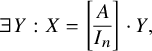
 $$\begin{align*}\mathcal{F}_1 = \left[\begin{array}{@{}c@{}} A\\ \hline I_n \end{array} \right], \quad \mathcal{F}_0 = X = \left[\begin{array}{@{}c@{}} X_1\\ \hline X_2 \end{array} \right], \end{align*}$$
where A is of size $ n \times n$
, X is of size
$ n \times n$
, X is of size $2n \times s$
and
$2n \times s$
and $X_1,X_2$
are of size
$X_1,X_2$
are of size $n\times s$
; with the additional condition that
$n\times s$
; with the additional condition that $\mathcal {F}_0$
has rank s and so X has an invertible
$\mathcal {F}_0$
has rank s and so X has an invertible $s\times s$
-minor. We also ask that
$s\times s$
-minor. We also ask that $(\mathcal {F}_0,\mathcal {F}_1)$
satisfy the following four conditions:
$(\mathcal {F}_0,\mathcal {F}_1)$
satisfy the following four conditions:
-
(1)
$\mathcal {F}_1^{\bot } = \mathcal {F}_1$
, -
(2)
$ \mathcal {F}_0 \subset \mathcal {F}_1$
, -
(3)
$(t - \pi )\mathcal {F}_0 = (0)$
, -
(4)
$(t + \pi ) \mathcal {F}_1 \subset \mathcal {F}_0$
.


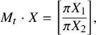
Observe that
 $$\begin{align*}M_t = \left[\begin{array}{@{}c|c@{}} 0_n & \pi_0I_n \\ \hline I_n & 0_n \end{array} \right] \end{align*}$$
of size $2n \times 2n $
is the matrix giving multiplication by t.
$2n \times 2n $
is the matrix giving multiplication by t.
Condition (1) (i.e., $\mathcal {F}_1$
is isotropic) translates to
$\mathcal {F}_1$
is isotropic) translates to $A^{t} = -J_nAJ_n$
. Condition (2) (i.e.,
$A^{t} = -J_nAJ_n$
. Condition (2) (i.e., $ \mathcal {F}_0 \subset \mathcal {F}_1$
) implies that the generators of
$ \mathcal {F}_0 \subset \mathcal {F}_1$
) implies that the generators of $\mathcal {F}_0$
can be expressed as a linear combination of the generators in
$\mathcal {F}_0$
can be expressed as a linear combination of the generators in $\mathcal {F}_1$
, which translates to
$\mathcal {F}_1$
, which translates to
 $$\begin{align*}\exists \, Y : X = \left[\begin{array}{@{}c@{}} A\\ \hline I_n \end{array} \right] \cdot Y, \end{align*}$$
where Y is of size $ n\times s$
. Thus, we have
$ n\times s$
. Thus, we have
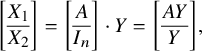 $$\begin{align*}\left[\begin{array}{@{}c@{}} X_1\\ \hline X_2 \end{array} \right] = \left[\begin{array}{@{}c@{}} A\\ \hline I_n \end{array} \right] \cdot Y = \left[\begin{array}{@{}c@{}} A Y\\ \hline Y \end{array} \right], \end{align*}$$
and so $ X_1 = AY$
and
$ X_1 = AY$
and $X_2 = Y.$
Condition (3) (i.e.,
$X_2 = Y.$
Condition (3) (i.e., $(t - \pi )\mathcal {F}_0 = (0)$
) is equivalent to
$(t - \pi )\mathcal {F}_0 = (0)$
) is equivalent to
 $$\begin{align*}M_t \cdot X = \left[\begin{array}{@{}c@{}} \pi X_1\\ \hline \pi X_2 \end{array} \right], \end{align*}$$
which amounts to
 $$\begin{align*}\left[\begin{array}{@{}c@{}} \pi_0 X_2\\ \hline X_1 \end{array} \right]= \left[\begin{array}{@{}c@{}} \pi X_1\\ \hline \pi X_2 \end{array} \right]. \end{align*}$$
Thus, $X_1 = \pi X_2$
, which translates to
$X_1 = \pi X_2$
, which translates to $A Y = \pi Y $
by condition
$A Y = \pi Y $
by condition $(2)$
. The last condition
$(2)$
. The last condition $(t + \pi ) \mathcal {F}_1 \subset \mathcal {F}_0$
translates to
$(t + \pi ) \mathcal {F}_1 \subset \mathcal {F}_0$
translates to
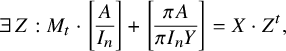 $$\begin{align*}\exists \, Z : M_t \cdot \left[\begin{array}{@{}c@{}} A \\ \hline I_n \end{array} \right] + \left[\begin{array}{@{}c@{}} \pi A \\ \hline \pi I_n Y \end{array} \right] = X \cdot Z^t, \end{align*}$$
where Z is of size $n\times s$
. This amounts to
$n\times s$
. This amounts to
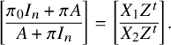 $$\begin{align*}\left[\begin{array}{@{}c@{}} \pi_0I_n + \pi A \\ \hline A + \pi I_n \end{array} \right] = \left[\begin{array}{@{}c@{}} X_1 Z^t \\ \hline X_2 Z^t \end{array} \right]. \end{align*}$$
From the above, we get $A + \pi I_n = X_2 Z^t$
, which by condition (2) translates to
$A + \pi I_n = X_2 Z^t$
, which by condition (2) translates to $ A = Y Z^t-\pi I_n. $
Thus, A can be expressed in terms of
$ A = Y Z^t-\pi I_n. $
Thus, A can be expressed in terms of $Y,Z$
. In addition, by condition (2) and in particular by the relations
$Y,Z$
. In addition, by condition (2) and in particular by the relations $ X_1 = AY$
and
$ X_1 = AY$
and $X_2 = Y$
, we deduce that the matrix X is given in terms of
$X_2 = Y$
, we deduce that the matrix X is given in terms of $Y,Z$
. Conversely, from
$Y,Z$
. Conversely, from $Y=X_2$
, we get that the matrix Y is given in terms of
$Y=X_2$
, we get that the matrix Y is given in terms of $A,X$
(Below we will also show that Z can be expressed in terms of
$A,X$
(Below we will also show that Z can be expressed in terms of $A,X$
).
$A,X$
).
Observe from $X_1 = \pi X_2$
that all the entries of
$X_1 = \pi X_2$
that all the entries of $X_1$
are in the maximal ideal and thus a minor involving entries of
$X_1$
are in the maximal ideal and thus a minor involving entries of $X_1$
cannot be a unit. Recall that the matrix X has an invertible
$X_1$
cannot be a unit. Recall that the matrix X has an invertible $s\times s$
-minor and
$s\times s$
-minor and $X_2=Y$
from condition (2). Thus, the matrix Y has a
$X_2=Y$
from condition (2). Thus, the matrix Y has a $s\times s$
-minor. Let
$s\times s$
-minor. Let
 $$\begin{align*}Y = \left[\begin{array}{ccc} y_{1,1} &\cdots & y_{1,s} \\ \vdots & \ddots & \vdots \\ y_{n,1} & \cdots & y_{n,s} \end{array}\right] , \quad Z = \left[\begin{array}{ccc} z_{1,1} &\cdots & z_{1,s} \\ \vdots & \ddots & \vdots \\ z_{n,1} & \cdots & z_{n,s} \end{array}\right] = \left[\begin{array}{ccc} \mathbf{z}_1 \ \cdots \ \mathbf{z}_s \end{array}\right], \end{align*}$$
and
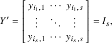 $$ \begin{align} Y'=\left[\begin{array}{ccc} y_{i_1,1} &\cdots & y_{i_1,s} \\ \vdots & \ddots & \vdots \\ y_{i_s,1} & \cdots & y_{i_s,s} \end{array}\right] = I_s, \end{align} $$
where $1 \leq i_k \leq n$
for
$1 \leq i_k \leq n$
for $k = 1, \dots ,s$
. Here, we want to mention how we can express Z in terms of
$k = 1, \dots ,s$
. Here, we want to mention how we can express Z in terms of $A,X$
. From the above, we have
$A,X$
. From the above, we have $Y Z^t=A+ \pi I_n$
and
$Y Z^t=A+ \pi I_n$
and
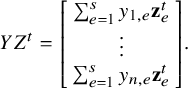 $$\begin{align*}Y Z^t = \left[\begin{array}{c} \sum^s_{e=1} y_{1,e} \mathbf{z}^t_e \\ \vdots \\ \sum^s_{e=1} y_{n,e} \mathbf{z}^t_e \end{array}\right]. \end{align*}$$
By using (4.1.1), for any $1 \leq k \leq s$
, the
$1 \leq k \leq s$
, the $i_k$
-th row of the matrix
$i_k$
-th row of the matrix $Y Z^t $
gives
$Y Z^t $
gives $\mathbf {z}^t_k $
. Since
$\mathbf {z}^t_k $
. Since $Y Z^t=A+ \pi I_n$
, we can easily see that the matrix Z can be expressed in terms of
$Y Z^t=A+ \pi I_n$
, we can easily see that the matrix Z can be expressed in terms of $A,X$
.
$A,X$
.
We replace A by $Y Z^t-\pi I_n$
. Hence, conditions (
$Y Z^t-\pi I_n$
. Hence, conditions ( $1$
) and (
$1$
) and ( $3$
) are equivalent to
$3$
) are equivalent to
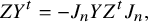 $$ \begin{align} Z Y^t &= -J_nY Z^tJ_n, \end{align} $$
 $$ \begin{align} Y Z^t Y &= 2 \pi Y. \qquad\quad \end{align} $$
From the above, we deduce the following.
Lemma 4.1. An affine chart $_1{\mathcal U}_{r,s}$
of
$_1{\mathcal U}_{r,s}$
of $\mathcal {M}$
around
$\mathcal {M}$
around $(\mathcal {F}_0, t \Lambda _m)$
is given by
$(\mathcal {F}_0, t \Lambda _m)$
is given by $\mathrm {Spec \, } O_F[Y , Z ]/\mathscr {I} $
, where
$\mathrm {Spec \, } O_F[Y , Z ]/\mathscr {I} $
, where
 $$\begin{align*}\mathscr{I} = (Y'-I_s,\ Z Y^t +J_nY Z^tJ_n,\ Y Z^t Y - 2 \pi Y) \end{align*}$$
and $Y'$
is a submatrix composed of s rows of Y (see the relation (4.1.1)).
$Y'$
is a submatrix composed of s rows of Y (see the relation (4.1.1)).
Note that the affine chart $_1{\mathcal U}_{r,s}$
of
$_1{\mathcal U}_{r,s}$
of $\mathcal {M}$
depends on the matrix
$\mathcal {M}$
depends on the matrix $Y'$
we fixed (see Remark 4.4). Our next goal is to give a simplification of the above equations (see Theorem 4.2). We first study the relation
$Y'$
we fixed (see Remark 4.4). Our next goal is to give a simplification of the above equations (see Theorem 4.2). We first study the relation $Z Y^t =-J_nY Z^tJ_n$
. Consider the matrix
$Z Y^t =-J_nY Z^tJ_n$
. Consider the matrix $P = (p_{i,j})$
of size
$P = (p_{i,j})$
of size $n=2m$
with
$n=2m$
with $P^t=-J_nPJ_n$
. By a direct calculation, we get
$P^t=-J_nPJ_n$
. By a direct calculation, we get
 $$\begin{align*}p_{i,j}=p_{n+1-j,n+1-i} \end{align*}$$
for $1\leq i, j\leq m$
or
$1\leq i, j\leq m$
or $m+1\leq i,j\leq n$
, and
$m+1\leq i,j\leq n$
, and
 $$\begin{align*}p_{i,j}=-p_{n+1-j,n+1-i} \end{align*}$$
for $1\leq i\leq m$
and
$1\leq i\leq m$
and $m+1\leq j\leq n$
, or
$m+1\leq j\leq n$
, or $1\leq j\leq m$
and
$1\leq j\leq m$
and $m+1\leq i\leq n$
. By using this observation and by setting
$m+1\leq i\leq n$
. By using this observation and by setting $P = Y Z^t$
, the relation
$P = Y Z^t$
, the relation $ Z Y^t=-J_nY Z^tJ_n$
gives
$ Z Y^t=-J_nY Z^tJ_n$
gives
 $$ \begin{align} \sum^s_{k=1} z_{i,k}y_{j,k} = \pm \sum^s_{k=1} z_{n+1-j,k}y_{n+1-i,k} \end{align} $$
for $1\leq i,j \leq n$
, where the different signs
$1\leq i,j \leq n$
, where the different signs $\pm $
depends on the position of
$\pm $
depends on the position of $i,j$
as above. Consider the following 2 cases:
$i,j$
as above. Consider the following 2 cases:
Case 1: Assume that $ 1\leq i_k \leq m$
for all
$ 1\leq i_k \leq m$
for all $k \in \{1,\dots ,s\}.$
By setting
$k \in \{1,\dots ,s\}.$
By setting $i = n+1-i_q $
and
$i = n+1-i_q $
and $j= i_p$
, the equation (4.1.4) gives
$j= i_p$
, the equation (4.1.4) gives $ z_{n+1-i_q,p} = -z_{n+1-i_p,q} .$
In particular, if
$ z_{n+1-i_q,p} = -z_{n+1-i_p,q} .$
In particular, if $p=q$
, we get
$p=q$
, we get $z_{n+1-i_p,p} = 0 $
for all
$z_{n+1-i_p,p} = 0 $
for all $p \in \{1,\dots ,s\}$
. By setting
$p \in \{1,\dots ,s\}$
. By setting $ d_{p,q} = z_{n+1-i_p,q}$
, we get the matrix
$ d_{p,q} = z_{n+1-i_p,q}$
, we get the matrix $D = (d_{p,q})_{p,q}$
of size
$D = (d_{p,q})_{p,q}$
of size $s \times s$
such that
$s \times s$
such that
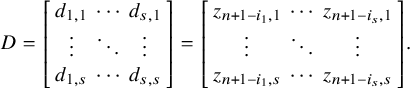 $$ \begin{align} D = \left[\begin{array}{ccc} d_{1,1} &\cdots & d_{s,1} \\ \vdots & \ddots & \vdots \\ d_{1,s} & \cdots & d_{s,s} \end{array}\right] = \left[\begin{array}{ccc} z_{n+1-i_1,1} &\cdots & z_{n+1-i_s,1} \\ \vdots & \ddots & \vdots \\ z_{n+1-i_1,s} & \cdots & z_{n+1-i_s,s} \end{array}\right]. \end{align} $$
The matrix D is skew-symmetric (i.e., $D = -D^t).$
Next, by setting
$D = -D^t).$
Next, by setting $j = i_k$
in (4.1.4), we obtain
$j = i_k$
in (4.1.4), we obtain
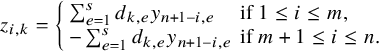 $$\begin{align*}z_{i,k} = \left\{ \begin{array}{ll} \sum^s_{e=1} d_{k,e}y_{n+1-i,e} & \mbox{if } 1 \leq i \leq m, \\ -\sum^s_{e=1} d_{k,e}y_{n+1-i,e} & \mbox{if } m+1\leq i \leq n. \end{array} \right. \end{align*}$$
Thus, we have $ Z = \widetilde {Y} \cdot D$
, where
$ Z = \widetilde {Y} \cdot D$
, where
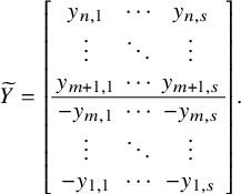 $$\begin{align*}\widetilde{Y} = \left[\begin{array}{ccc} y_{n,1} & \cdots & y_{n,s} \\ \vdots & \ddots & \vdots \\ y_{m+1,1} & \cdots & y_{m+1,s} \\ \hline -y_{m,1} & \cdots & -y_{m,s} \\ \vdots & \ddots & \vdots \\ -y_{1,1} & \cdots & -y_{1,s} \\ \end{array}\right]. \end{align*}$$
Therefore, in this case, the equations (4.1.4) give $ Z = \widetilde {Y} \cdot D $
.
$ Z = \widetilde {Y} \cdot D $
.
Case 2: In general, we let $ 1 \leq t \leq s$
and assume that
$ 1 \leq t \leq s$
and assume that
 $$\begin{align*}1\leq i_1, \dots, i_t \leq m \quad \text{and} \quad m+1\leq i_{t+1}, \dots, i_s \leq n. \end{align*}$$
By setting $d_{p,q} = z_{n+1-i_p,q}$
and using the same arguments as above, we get the matrix
$d_{p,q} = z_{n+1-i_p,q}$
and using the same arguments as above, we get the matrix $D = (d_{p,q})_{p,q}$
of size
$D = (d_{p,q})_{p,q}$
of size $s \times s$
such that
$s \times s$
such that
 $$\begin{align*}d_{p,q}=-d_{q,p} \end{align*}$$
for $1\leq p, q \leq t$
or
$1\leq p, q \leq t$
or $t+1\leq p,q\leq n$
, and
$t+1\leq p,q\leq n$
, and
 $$\begin{align*}d_{p,q}=d_{q,p} \end{align*}$$
for $1\leq p\leq t$
and
$1\leq p\leq t$
and $t+1\leq q\leq n$
, or
$t+1\leq q\leq n$
, or $1\leq q\leq t$
and
$1\leq q\leq t$
and $t+1\leq p\leq n$
. Next, by setting
$t+1\leq p\leq n$
. Next, by setting $j = i_k$
in (4.1.4) for
$j = i_k$
in (4.1.4) for $1\leq k \leq t$
, we obtain
$1\leq k \leq t$
, we obtain
 $$\begin{align*}z_{i,k} = \left\{ \begin{array}{ll} \sum^s_{e=1} d_{k,e}y_{n+1-i,e} & \mbox{if } 1 \leq i \leq m, \\ -\sum^s_{e=1} d_{k,e}y_{n+1-i,e} & \mbox{if } m+1\leq i \leq n. \end{array} \right. \end{align*}$$
Also, by setting $j = i_k$
for
$j = i_k$
for $t+1\leq k \leq s$
, we get
$t+1\leq k \leq s$
, we get
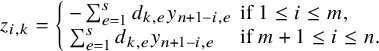 $$\begin{align*}z_{i,k} = \left\{ \begin{array}{ll} -\sum^s_{e=1} d_{k,e}y_{n+1-i,e} & \mbox{if } 1 \leq i \leq m, \\ \sum^s_{e=1} d_{k,e}y_{n+1-i,e} & \mbox{if } m+1\leq i \leq n. \end{array} \right. \end{align*}$$
From the above, we have $ Z = \widetilde {Y} \cdot \widetilde {D}$
, where
$ Z = \widetilde {Y} \cdot \widetilde {D}$
, where $\widetilde {D} = (\widetilde {d}_{i,j})_{i,j}$
is the
$\widetilde {D} = (\widetilde {d}_{i,j})_{i,j}$
is the $s \times s$
matrix defined as
$s \times s$
matrix defined as
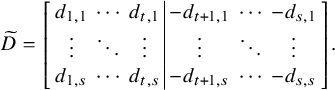 $$\begin{align*}\widetilde{D} = \left[\begin{array}{ccc|ccc} d_{1,1} & \cdots & d_{t,1} & -d_{t+1,1} & \cdots & -d_{s,1}\\ \vdots & \ddots & \vdots & \vdots & \ddots & \vdots \\ d_{1,s} & \cdots & d_{t,s} & -d_{t+1,s} & \cdots & -d_{s,s}\\ \end{array}\right]. \end{align*}$$
It is easy to see that the matrix $ \widetilde {D}$
is skew symmetric (i.e.,
$ \widetilde {D}$
is skew symmetric (i.e., $\widetilde {d}_{i,j} = - \widetilde {d}_{j,i}).$
In particular, we have the following 4 cases: when
$\widetilde {d}_{i,j} = - \widetilde {d}_{j,i}).$
In particular, we have the following 4 cases: when $1 \leq i,j \leq t$
, we have
$1 \leq i,j \leq t$
, we have $ \widetilde {d}_{i,j} = d_{i,j} = -d_{j,i} = - \widetilde {d}_{j,i}$
. For
$ \widetilde {d}_{i,j} = d_{i,j} = -d_{j,i} = - \widetilde {d}_{j,i}$
. For $1 \leq i \leq t$
and
$1 \leq i \leq t$
and $t+1 \leq j \leq s $
, we have
$t+1 \leq j \leq s $
, we have $ \widetilde {d}_{i,j} = -d_{i,j} = -d_{j,i} = - \widetilde {d}_{j,i}$
. When
$ \widetilde {d}_{i,j} = -d_{i,j} = -d_{j,i} = - \widetilde {d}_{j,i}$
. When $1 \leq j \leq t$
and
$1 \leq j \leq t$
and $t+1 \leq i \leq s $
, we get
$t+1 \leq i \leq s $
, we get $ \widetilde {d}_{i,j} = d_{i,j} = d_{j,i} = - \widetilde {d}_{j,i}$
. Lastly, for
$ \widetilde {d}_{i,j} = d_{i,j} = d_{j,i} = - \widetilde {d}_{j,i}$
. Lastly, for $t+1 \leq i,j \leq s$
, we obtain
$t+1 \leq i,j \leq s$
, we obtain $ \widetilde {d}_{i,j} = -d_{i,j} = d_{j,i} = - \widetilde {d}_{j,i}$
.
$ \widetilde {d}_{i,j} = -d_{i,j} = d_{j,i} = - \widetilde {d}_{j,i}$
.
Combining the above cases, for any $1\leq i_1,\dots , i_s\leq n$
, the equations (4.1.4) show that there exists a skew symmetric matrix
$1\leq i_1,\dots , i_s\leq n$
, the equations (4.1.4) show that there exists a skew symmetric matrix $\mathcal {D}$
of size
$\mathcal {D}$
of size $s \times s$
such that
$s \times s$
such that
 $$\begin{align*}Z = \widetilde{Y} \cdot \mathcal{D}. \end{align*}$$
By abuse of notation, write $ D$
for
$ D$
for $ \mathcal {D}$
. Next, define
$ \mathcal {D}$
. Next, define $ Q : =\widetilde {Y}^t \cdot Y $
of size
$ Q : =\widetilde {Y}^t \cdot Y $
of size $ s \times s.$
Note that
$ s \times s.$
Note that $ Q^t = -Q.$
We are now ready to show the following:
$ Q^t = -Q.$
We are now ready to show the following:
Theorem 4.2. For any signature $(r,s)$
, there is an affine chart
$(r,s)$
, there is an affine chart $_1{\mathcal U}_{r,s} \subset \mathcal {M}$
which is isomorphic to
$_1{\mathcal U}_{r,s} \subset \mathcal {M}$
which is isomorphic to $\mathrm {Spec \, } O_F[ D, Y]/I $
, where
$\mathrm {Spec \, } O_F[ D, Y]/I $
, where
 $$\begin{align*}I = \left(Y'-I_s,\ D+D^t,\ D\cdot Q + 2 \pi I_s\right) \end{align*}$$
for some choice of $Y'$
.
$Y'$
.
Proof. Recall from Lemma 4.1 that ${\mathcal U} = \mathrm {Spec \, } O_F[Y , Z ]/\mathscr {I} $
, where
${\mathcal U} = \mathrm {Spec \, } O_F[Y , Z ]/\mathscr {I} $
, where
 $$\begin{align*}\mathscr{I} = (Y'-I_s,\ Z Y^t +J_nY Z^tJ_n,\ Y Z^t Y - 2 \pi Y). \end{align*}$$
From the above discussion, we have that the relation $Z Y^t =-J_nY Z^tJ_n $
gives
$Z Y^t =-J_nY Z^tJ_n $
gives $ Z = \widetilde {Y} \cdot D$
. Thus, it suffices to focus on the relation
$ Z = \widetilde {Y} \cdot D$
. Thus, it suffices to focus on the relation $ Y Z^t Y - 2 \pi Y=0$
. Observe that
$ Y Z^t Y - 2 \pi Y=0$
. Observe that $ Y \cdot Z^t \cdot Y =- Y \cdot D \cdot Q.$
Thus,
$ Y \cdot Z^t \cdot Y =- Y \cdot D \cdot Q.$
Thus,
 $$\begin{align*}Y Z^t Y - 2 \pi Y = -Y\cdot( D \cdot Q + 2 \pi I_s)=0. \end{align*}$$
Now, by using the relation with the minors (4.1.1), we can easily see that the relation $Y Z^t Y - 2 \pi Y=0$
gives
$Y Z^t Y - 2 \pi Y=0$
gives $D \cdot Q + 2 \pi I_s=0.$
Therefore,
$D \cdot Q + 2 \pi I_s=0.$
Therefore, $_1{\mathcal U}_{r,s}$
is isomorphic to
$_1{\mathcal U}_{r,s}$
is isomorphic to
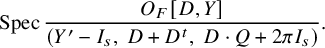 $$\begin{align*}\mathrm{Spec \, } \frac{O_F[D,Y]}{\left(Y'-I_s,\ D+D^t, \ D\cdot Q + 2 \pi I_s\right)}.\\[-44pt] \end{align*}$$
In particular, when the signature $(r,s)=(n-2,2)$
, we have
$(r,s)=(n-2,2)$
, we have
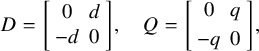 $$\begin{align*}D=\left[\begin{array}{cc} 0&d\\ -d&0 \end{array}\right],\quad Q=\left[\begin{array}{cc} 0&q\\[2pt] -q&0 \end{array}\right], \end{align*}$$
where $d=d_{2,1}=-d_{12}$
and
$d=d_{2,1}=-d_{12}$
and $q=\sum ^m_{j=1}y_{n+1-j,1}y_{j,2} - \sum ^n_{j=m+1}y_{n+1-j,1}y_{j,2}$
.
$q=\sum ^m_{j=1}y_{n+1-j,1}y_{j,2} - \sum ^n_{j=m+1}y_{n+1-j,1}y_{j,2}$
.
Corollary 4.3. When $(r,s)=(n-2,2)$
, there is an affine chart
$(r,s)=(n-2,2)$
, there is an affine chart $_1\mathcal {U}_{r,s} \subset \mathcal {M}$
which is isomorphic to
$_1\mathcal {U}_{r,s} \subset \mathcal {M}$
which is isomorphic to $V(I) = \mathrm {Spec \, } O_F[d,(y_{i,1})_{1 \leq i \leq n},(y_{i,2})_{1 \leq i \leq n} ]/ I$
, where
$V(I) = \mathrm {Spec \, } O_F[d,(y_{i,1})_{1 \leq i \leq n},(y_{i,2})_{1 \leq i \leq n} ]/ I$
, where
 $$\begin{align*}I= ( y_{i_0,1}-1,\,\, y_{j_0,2} -1 ,\,\,y_{j_0,1},\,y_{i_0,2},\,\, d(\sum^m_{j=1}y_{n+1-j,1}y_{j,2} - \sum^n_{j=m+1}y_{n+1-j,1}y_{j,2}) -2 \pi) \end{align*}$$
for some $1\leq i_0,j_0 \leq n$
.
$1\leq i_0,j_0 \leq n$
.
Remark 4.4. Recall that $_1{\mathcal U}_{r,s}$
is an affine chart around
$_1{\mathcal U}_{r,s}$
is an affine chart around $(\mathcal {F}_0, t\Lambda _m)$
. Note that for different choices of
$(\mathcal {F}_0, t\Lambda _m)$
. Note that for different choices of $Y'$
, we get different equations from
$Y'$
, we get different equations from $D\cdot Q =- 2 \pi I_s$
and so different affine charts
$D\cdot Q =- 2 \pi I_s$
and so different affine charts $_1{\mathcal U}_{r,s}$
which in general are not isomorphic. For instance, in Corollary 4.3, there are two different
$_1{\mathcal U}_{r,s}$
which in general are not isomorphic. For instance, in Corollary 4.3, there are two different $V(I)$
up to isomorphism when we choose different places for
$V(I)$
up to isomorphism when we choose different places for $i_0, j_0$
(see §5.2 for more details). In Proposition 5.2, we show that for any such a choice, the affine scheme
$i_0, j_0$
(see §5.2 for more details). In Proposition 5.2, we show that for any such a choice, the affine scheme $V(I)$
has semi-stable reduction over
$V(I)$
has semi-stable reduction over $O_F$
.
$O_F$
.
4.2 An Affine Chart
$_2{\mathcal U}_{r,s}$

Keep the same notation as above. As in [Reference Pappas and Rapoport18], we set $\Lambda _m=\Lambda '\oplus \Lambda "$
, where
$\Lambda _m=\Lambda '\oplus \Lambda "$
, where
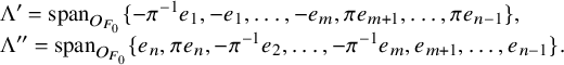 $$\begin{align*}\begin{array}{l} \Lambda'=\text{span}_{O_{F_0}}\{-\pi^{-1}e_1, -e_1,\dots,-e_m,\pi e_{m+1},\dots, \pi e_{n-1}\},\\ \Lambda"=\text{span}_{O_{F_0}}\{e_n, \pi e_n, -\pi^{-1}e_2, \dots, -\pi^{-1}e_m, e_{m+1}, \dots, e_{n-1}\}. \end{array} \end{align*}$$
In this subsection, we are going to write down the equations that define $\mathcal {M}$
in a neighborhood
$\mathcal {M}$
in a neighborhood $_2\mathcal {U}_{r,s}$
of
$_2\mathcal {U}_{r,s}$
of $(\mathcal {F}_0, \Lambda ')$
.
$(\mathcal {F}_0, \Lambda ')$
.
The matrix of the form $(\ ,\ )$
in this basis is
$(\ ,\ )$
in this basis is
 $$\begin{align*}\left[ \begin{array}{c|c} 0_n & S\\ \hline S^t & 0_n \end{array} \right],\end{align*}$$
where S is the skew-symmetric matrix of size n given by
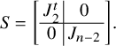 $$\begin{align*}S=\left[ \begin{array}{c|c} J_2^t & 0\\ \hline 0 & J_{n-2} \end{array} \right]. \end{align*}$$
Observe that $S^2=-I_n$
since
$S^2=-I_n$
since $J_n^2=-I_n$
. For any point
$J_n^2=-I_n$
. For any point $(\mathcal {F}_0,\mathcal {F}_1)\in \mathcal {M}$
, we ask that
$(\mathcal {F}_0,\mathcal {F}_1)\in \mathcal {M}$
, we ask that $ (\mathcal {F}_0,\mathcal {F}_1)$
satisfy the following conditions:
$ (\mathcal {F}_0,\mathcal {F}_1)$
satisfy the following conditions:
-
(1)
$\mathcal {F}_1^{\bot } = \mathcal {F}_1$
, -
(2)
$ \mathcal {F}_0 \subset \mathcal {F}_1$
, -
(3)
$(t - \pi )\mathcal {F}_0 = (0)$
, -
(4)
$(t + \pi ) \mathcal {F}_1 \subset \mathcal {F}_0$
.


Similar to §4.1, we consider
 $$\begin{align*}\mathcal{F}_1=\left[\begin{array}{c} I_n\\ \hline A \end{array} \right],\quad \mathcal{F}_0=X=\left[\begin{array}{c} X_1\\ \hline X_2 \end{array} \right], \end{align*}$$
where $I_n, A$
are
$I_n, A$
are $n\times n$
-matrices, and
$n\times n$
-matrices, and $X_1, X_2$
are
$X_1, X_2$
are $n\times s$
-matrices. Recall that
$n\times s$
-matrices. Recall that $\mathcal {F}_0$
has rank s, so X has a no-vanishing
$\mathcal {F}_0$
has rank s, so X has a no-vanishing $s\times s$
minor. Write down the matrix A by
$s\times s$
minor. Write down the matrix A by
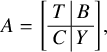 $$\begin{align*}A=\left[\begin{array}{c|c} T & B\\ \hline C & Y \end{array} \right], \end{align*}$$
where T is a $2\times 2$
-matrix, B (resp. C) is a
$2\times 2$
-matrix, B (resp. C) is a $2\times (n-2)$
-matrix (resp.
$2\times (n-2)$
-matrix (resp. $(n-2)\times 2$
-matrix) and Y is of size
$(n-2)\times 2$
-matrix) and Y is of size $(n-2)\times (n-2)$
. Then condition (1) is equivalent to
$(n-2)\times (n-2)$
. Then condition (1) is equivalent to $A^t S=SA$
. This translates to
$A^t S=SA$
. This translates to
 $$\begin{align*}T^t=-J_2TJ_2,\quad C=J_{n-2}B^tJ_2,\quad Y^t=-J_{n-2}YJ_{n-2}. \end{align*}$$
Note that the first equation immediately gives $T=\text {diag}(x,x)$
for some variable x, and the second equation shows that C is given in terms of B. Condition (2) is equivalent to
$T=\text {diag}(x,x)$
for some variable x, and the second equation shows that C is given in terms of B. Condition (2) is equivalent to
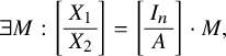 $$\begin{align*}\exists M: \left[\begin{array}{c} X_1\\ \hline X_2 \end{array} \right]= \left[\begin{array}{c} I_n\\ \hline A \end{array} \right]\cdot M, \end{align*}$$
where M is a $n\times s$
-matrix. This amounts to
$n\times s$
-matrix. This amounts to $X_1=M, X_2=AM$
. Let
$X_1=M, X_2=AM$
. Let
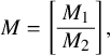 $$\begin{align*}M=\left[\begin{array}{c} M_1\\ \hline M_2 \end{array} \right], \end{align*}$$
where $M_1$
is of size
$M_1$
is of size $2\times s$
and
$2\times s$
and $M_2$
is of size
$M_2$
is of size $(n-2)\times s$
. We can see that
$(n-2)\times s$
. We can see that $X_1, X_2$
can be expressed in terms of
$X_1, X_2$
can be expressed in terms of $A, M_1, M_2$
. More precisely, we get
$A, M_1, M_2$
. More precisely, we get
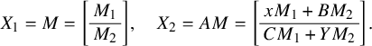 $$\begin{align*}X_1=M=\left[\begin{array}{c} M_1\\ \hline M_2 \end{array} \right],\quad X_2=AM=\left[\begin{array}{c} xM_1+BM_2\\ \hline CM_1+YM_2 \end{array} \right]. \end{align*}$$
The map $t: \Lambda _m\rightarrow \Lambda _m$
is represented by the matrix
$t: \Lambda _m\rightarrow \Lambda _m$
is represented by the matrix
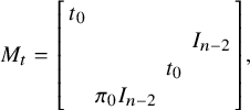 $$\begin{align*}M_t=\left[\begin{array}{cccc} t_0&&&\\ &&& I_{n-2}\\ && t_0 &\\ & \pi_0 I_{n-2} && \end{array} \right], \end{align*}$$
where $t_0$
is the
$t_0$
is the $2\times 2$
-antidiag matirx
$2\times 2$
-antidiag matirx $\left [\begin {array}{cc} & \pi _0\\ 1& \end {array} \right ]$
. Condition (3) translates to
$\left [\begin {array}{cc} & \pi _0\\ 1& \end {array} \right ]$
. Condition (3) translates to
 $$\begin{align*}M_t\cdot\left[ \begin{array}{c} X_1\\ \hline X_2 \end{array}\right]=\left[ \begin{array}{c} \pi X_1\\ \hline \pi X_2 \end{array}\right]. \end{align*}$$
By setting $B_i$
as the i-th row of B and by using condition (2), the above relation amounts to
$B_i$
as the i-th row of B and by using condition (2), the above relation amounts to
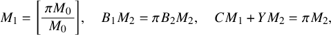 $$\begin{align*}M_1=\left[\begin{array}{c} \pi M_0\\ \hline M_0 \end{array} \right],\quad B_1M_2=\pi B_2M_2,\quad CM_1+YM_2=\pi M_2, \end{align*}$$
where $M_0$
is the second row of
$M_0$
is the second row of $M_1$
. Finally, condition (4) is equivalent to
$M_1$
. Finally, condition (4) is equivalent to
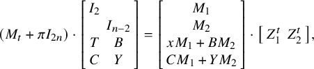 $$\begin{align*}(M_t+\pi I_{2n})\cdot \left[\begin{array}{cc} I_2 &\\ & I_{n-2}\\ T & B\\ C & Y \end{array} \right]=\left[\begin{array}{c} M_1\\ M_2\\ xM_1+BM_2\\ CM_1+YM_2 \end{array} \right]\cdot \left[\begin{array}{cc} Z_1^t & Z_2^t \end{array} \right], \end{align*}$$
where $Z_1$
is of size
$Z_1$
is of size $2\times s$
and
$2\times s$
and $Z_2$
is of size
$Z_2$
is of size $(n-2)\times s$
. This, in turn, gives
$(n-2)\times s$
. This, in turn, gives
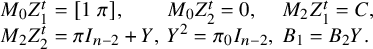 $$\begin{align*}\begin{array}{lll} M_0Z_1^t=[1\ \pi], & M_0Z_2^t=0, & M_2Z_1^t=C,\\ M_2Z_2^t=\pi I_{n-2} +Y, & Y^2= \pi_0 I_{n-2}, & B_1=B_2Y. \end{array} \end{align*}$$
From the above equations, we can see that A is given in terms of $x, C, Y$
by condition (1). Note that
$x, C, Y$
by condition (1). Note that $C=M_2Z_1^t$
, and
$C=M_2Z_1^t$
, and $Y=M_2Z_2^t-\pi I_{n-2}$
by condition (4). Thus, the matrix A is given in terms of
$Y=M_2Z_2^t-\pi I_{n-2}$
by condition (4). Thus, the matrix A is given in terms of $M, Z_1, Z_2$
and a variable x. Meanwhile, we have
$M, Z_1, Z_2$
and a variable x. Meanwhile, we have $X_1=M, X_2=AM$
by condition (2), so that
$X_1=M, X_2=AM$
by condition (2), so that $X_1, X_2$
are also given in terms of
$X_1, X_2$
are also given in terms of $M, Z_1, Z_2$
. However, we have
$M, Z_1, Z_2$
. However, we have $M=X_1$
, and we claim that
$M=X_1$
, and we claim that $Z_1, Z_2$
can be expressed in terms of
$Z_1, Z_2$
can be expressed in terms of $A, X_1, X_2$
(we will show this later in this section).
$A, X_1, X_2$
(we will show this later in this section).
Before we move on, let us simplify our equations first. By replacing $Y=M_2Z_2^t-\pi I_{n-2}$
, the equation
$Y=M_2Z_2^t-\pi I_{n-2}$
, the equation $Y^t=-J_{n-2}YJ_{n-2}$
from condition (1) amounts to
$Y^t=-J_{n-2}YJ_{n-2}$
from condition (1) amounts to $(M_2Z_2^t)^t=-J_{n-2}(M_2Z_2^t)J_{n-2}$
, and the equations that involve Y from condition (3), (4) translate to
$(M_2Z_2^t)^t=-J_{n-2}(M_2Z_2^t)J_{n-2}$
, and the equations that involve Y from condition (3), (4) translate to
 $$\begin{align*}CM_1+(M_2Z_2^t)M_2=2\pi M_2,\quad (M_2Z_2^t)^2=2\pi(M_2Z_2^t),\quad B_1+\pi B_2=B_2(M_2Z_2^t). \end{align*}$$
Finally, we replace C by $M_2Z_1^t$
, and deduce the following.
$M_2Z_1^t$
, and deduce the following.
Lemma 4.5. The affine chart $_2{\mathcal U}_{r,s}$
of
$_2{\mathcal U}_{r,s}$
of $\mathcal {M}$
around
$\mathcal {M}$
around $(\mathcal {F}_0, \Lambda ')$
is given by
$(\mathcal {F}_0, \Lambda ')$
is given by
 $$\begin{align*}\mathrm{Spec \, } O_F[x, B, M_0, M_2, Z_1, Z_2]/\mathscr{I}, \end{align*}$$
where $\mathscr {I}$
is the ideal generated by the entries of following equations:
$\mathscr {I}$
is the ideal generated by the entries of following equations:
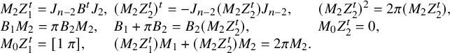 $$\begin{align*}\begin{array}{lll} M_2Z_1^t=J_{n-2}B^tJ_2, & (M_2Z_2^t)^t=-J_{n-2}(M_2Z_2^t)J_{n-2}, & (M_2Z_2^t)^2=2\pi(M_2Z_2^t),\\ B_1M_2=\pi B_2M_2, &B_1+\pi B_2=B_2(M_2Z_2^t), & M_0Z_2^t=0,\\ M_0Z_1^t=[1\ \pi], &(M_2Z_1^t)M_1+(M_2Z_2^t)M_2=2\pi M_2. & \end{array} \end{align*}$$
Here, $B_i$
is the i-th row of B for
$B_i$
is the i-th row of B for $i=1,2$
.
$i=1,2$
.
Remark 4.6. Condition (3) also gives the equations:
 $$\begin{align*}BC=0,\quad Ct_0+YC=0. \end{align*}$$
In [Reference Pappas and Rapoport18, §5.3], the authors show that these two equations are automatically true if $B,C,Y$
satisfy
$B,C,Y$
satisfy
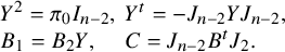 $$\begin{align*}\begin{array}{ll} Y^2=\pi_0 I_{n-2}, & Y^t=-J_{n-2}YJ_{n-2},\\ B_1=B_2Y, & C=J_{n-2}B^tJ_2. \end{array} \end{align*}$$
4.2.1 The case
$(r,s)=(n-1,1)$

In this and the next subsection, our goal is to give a simplification of the equations in Lemma 4.5. We first consider the affine chart $_2\mathcal {U}_{n-1,1} \subset \mathcal {M}$
for the signature
$_2\mathcal {U}_{n-1,1} \subset \mathcal {M}$
for the signature $(n-1,1)$
. Note that
$(n-1,1)$
. Note that $M_0$
is of size
$M_0$
is of size $1\times 1$
in this case. Since
$1\times 1$
in this case. Since
 $$\begin{align*}M_0 Z_1^t=[1\ \pi]\neq 0, \end{align*}$$
we get $M_0\neq 0$
. Without loss of generality, we assume
$M_0\neq 0$
. Without loss of generality, we assume $M_0=1$
as rank(
$M_0=1$
as rank( $\mathcal {F}_0$
)=1.
$\mathcal {F}_0$
)=1.
Theorem 4.7. When the signature $(r,s)=(n-1,1)$
, the affine chart
$(r,s)=(n-1,1)$
, the affine chart $_2\mathcal {U}_{n-1,1}$
is smooth and isomorphic to
$_2\mathcal {U}_{n-1,1}$
is smooth and isomorphic to $\mathbb {A}_{O_F}^{n-1}$
.
$\mathbb {A}_{O_F}^{n-1}$
.
Proof. From $M_0Z_1^t=[1\ \pi ]$
,
$M_0Z_1^t=[1\ \pi ]$
, $M_0Z_2^t=0$
, we obtain
$M_0Z_2^t=0$
, we obtain
 $$\begin{align*}Z_1^t=\left[\begin{array}{cc} 1& \pi\\ \end{array} \right],\quad Z_2^t=0. \end{align*}$$
Let $M_2=[a_1\ \cdots \ a_{n-2}]^t$
be an
$M_2=[a_1\ \cdots \ a_{n-2}]^t$
be an $(n-2)\times 1$
vector. Then
$(n-2)\times 1$
vector. Then $C=M_2Z_1^t$
amounts to
$C=M_2Z_1^t$
amounts to
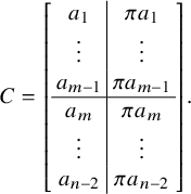 $$\begin{align*}C=\left[\begin{array}{c|c} a_1 &\pi a_1\\ \vdots & \vdots \\ a_{m-1} &\pi a_{m-1}\\ \hline a_{m} &\pi a_{m}\\ \vdots & \vdots \\ a_{n-2}& \pi a_{n-2} \end{array} \right]. \end{align*}$$
Also, from $B=J_2C^tJ_{n-2}$
, we get
$B=J_2C^tJ_{n-2}$
, we get
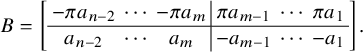 $$\begin{align*}B=\left[\begin{array}{ccc|ccc} -\pi a_{n-2} &\cdots &-\pi a_m& \pi a_{m-1}& \cdots &\pi a_1 \\ \hline a_{n-2} &\cdots & a_m& -a_{m-1}& \cdots & -a_1 \end{array}\right]. \end{align*}$$
It is easy to see that the relation $Y=M_2Z_2^t-\pi I_{n-2}$
gives
$Y=M_2Z_2^t-\pi I_{n-2}$
gives $Y=-\pi I_{n-2}$
and
$Y=-\pi I_{n-2}$
and $B_1+\pi B_2=B_2(M_2Z_2^t)=0$
. Finally, we check that
$B_1+\pi B_2=B_2(M_2Z_2^t)=0$
. Finally, we check that
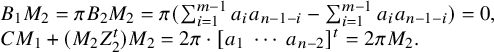 $$\begin{align*}\begin{array}{l} B_1M_2=\pi B_2M_2=\pi(\sum_{i=1}^{m-1}a_ia_{n-1-i}-\sum_{i=1}^{m-1}a_ia_{n-1-i})=0,\\ CM_1+(M_2Z_2^t)M_2=2\pi\cdot [a_1\ \cdots\ a_{n-2}]^t=2\pi M_2. \end{array} \end{align*}$$
From the above, the conditions on the $a_i$
are automatically satisfied. We deduce that the affine chart
$a_i$
are automatically satisfied. We deduce that the affine chart $_2\mathcal {U}_{n-1,1}$
is isomorphic to
$_2\mathcal {U}_{n-1,1}$
is isomorphic to
 $$\begin{align*}\mathrm{Spec \, } O_F[x, a_1, \dots, a_{n-2}]=\mathbb{A}_{O_F}^{n-1}.\\[-38pt] \end{align*}$$
4.2.2 The cases for
$s\geq 2$

In this subsection, we consider the explicit equations of $_2\mathcal {U}_{r,s}$
for the signature
$_2\mathcal {U}_{r,s}$
for the signature $(r,s)$
with
$(r,s)$
with $s\geq 2$
. Observe that
$s\geq 2$
. Observe that $\mathcal {F}_1=\{v+A(v)\mid v\in \Lambda '\otimes {\mathcal O}_S \}$
. In the special fiber (where
$\mathcal {F}_1=\{v+A(v)\mid v\in \Lambda '\otimes {\mathcal O}_S \}$
. In the special fiber (where ${\mathcal O}_S=k$
), we have
${\mathcal O}_S=k$
), we have $t\mathcal {F}_1\subset \mathcal {F}_0$
, and
$t\mathcal {F}_1\subset \mathcal {F}_0$
, and $t(\Lambda '\otimes k)=\text {span}_{O_{F_0}}\{-e_1\}$
, which implies
$t(\Lambda '\otimes k)=\text {span}_{O_{F_0}}\{-e_1\}$
, which implies $-e_1+tA(v)\in \mathcal {F}_0$
. Since
$-e_1+tA(v)\in \mathcal {F}_0$
. Since
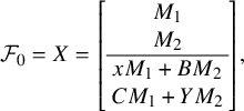 $$\begin{align*}\mathcal{F}_0=X=\left[\begin{array}{c} M_1\\ M_2 \\ \hline xM_1+BM_2\\ CM_1+YM_2 \end{array} \right], \end{align*}$$
we can always assume that $-e_1+tA(v)$
is the first generating element of
$-e_1+tA(v)$
is the first generating element of $\mathcal {F}_0$
. In the matrix language, this is equivalent to assume that the second row of X (i.e.,
$\mathcal {F}_0$
. In the matrix language, this is equivalent to assume that the second row of X (i.e., $M_0$
) is equal to
$M_0$
) is equal to $[1\ 0 \cdots 0]$
. Thus, we have
$[1\ 0 \cdots 0]$
. Thus, we have
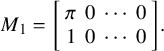 $$\begin{align*}M_1=\left[\begin{array}{cccc} \pi & 0&\cdots& 0\\ 1& 0&\cdots &0 \end{array} \right]. \end{align*}$$
By using $M_0Z_1^t=[1 \ \pi ]$
,
$M_0Z_1^t=[1 \ \pi ]$
, $M_0Z_2^t=0$
, we set
$M_0Z_2^t=0$
, we set
 $$\begin{align*}Z_1^t=\left[\begin{array}{cc} 1& \pi \\ z_{1,2} & z_{2,2}\\ \vdots &\vdots\\ z_{1,s} & z_{2,s} \end{array} \right], \quad Z_2^t=\left[\begin{array}{ccc} 0&\cdots & 0 \\ z_{1,2}'&\cdots & z_{n-2,2}'\\ \vdots & \ddots & \vdots \\ z_{1,s}'&\cdots & z_{n-2,s}' \end{array} \right], \end{align*}$$
and
 $$\begin{align*}M_2=\left[\begin{array}{cccc} \mathbf{a_1} & \cdots &\mathbf{a_s} \end{array}\right]= \left[\begin{array}{ccc} a_{1,1}& \cdots & a_{1,s} \\ \vdots & \ddots &\vdots \\ a_{n-2,1} & \cdots & a_{n-2,s} \end{array} \right]. \end{align*}$$
We claim that $Z_1, Z_2$
can be expressed in terms of
$Z_1, Z_2$
can be expressed in terms of $A, X_1, X_2$
. Observe from
$A, X_1, X_2$
. Observe from $CM_1+YM_2=\pi M_2$
that all the entries of
$CM_1+YM_2=\pi M_2$
that all the entries of $CM_1+YM_2$
are in the maximal ideal, and thus a minor involving entries of
$CM_1+YM_2$
are in the maximal ideal, and thus a minor involving entries of $CM_1+YM_2$
cannot be a unit. Similarly, the entries of the first row of
$CM_1+YM_2$
cannot be a unit. Similarly, the entries of the first row of $xM_1+BM_2$
are also in the maximal ideal. By replacing the order of basis
$xM_1+BM_2$
are also in the maximal ideal. By replacing the order of basis $\{\pi e_m,\dots , \pi e_n\}$
if necessary, we can assume that the matrix
$\{\pi e_m,\dots , \pi e_n\}$
if necessary, we can assume that the matrix $M_2$
has an invertible
$M_2$
has an invertible $(s-1)\times (s-1)$
-minor. Let
$(s-1)\times (s-1)$
-minor. Let $M_2'$
be a submatrix of
$M_2'$
be a submatrix of $M_2$
composing
$M_2$
composing $(s-1)$
rows along with the corresponding s columns. We set
$(s-1)$
rows along with the corresponding s columns. We set
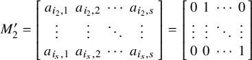 $$\begin{align*}M_2'=\left[\begin{array}{cccc} a_{i_2,1}& a_{i_2,2} &\cdots & a_{i_2,s} \\ \vdots & \vdots &\ddots &\vdots \\ a_{i_s,1} & a_{i_s,2}&\cdots & a_{i_s,s} \end{array} \right]= \left[\begin{array}{cccc} 0& 1 & \cdots & 0 \\ \vdots & \vdots & \ddots &\vdots \\ 0 & 0 & \cdots & 1 \end{array} \right] \end{align*}$$
for $1\leq i_2, \cdots , i_s\leq n-2$
. Consider the matrix
$1\leq i_2, \cdots , i_s\leq n-2$
. Consider the matrix $C=M_2Z_1^t$
. We have
$C=M_2Z_1^t$
. We have
 $$\begin{align*}C=\left[\begin{array}{cc} \mathbf{a_1}+z_{1,2}\mathbf{a_2}+\cdots +z_{1,s}\mathbf{a_s} & \pi \mathbf{a_1}+z_{2,2}\mathbf{a_2}+\cdots +z_{2,s}\mathbf{a_s} \end{array}\right]. \end{align*}$$
By setting $i=i_2, \dots , i_s$
, it is easy to see that
$i=i_2, \dots , i_s$
, it is easy to see that $Z_1$
can be expressed in terms of C. Similarly,
$Z_1$
can be expressed in terms of C. Similarly, $Z_2$
can be expressed in terms of Y as
$Z_2$
can be expressed in terms of Y as $M_2Z_2^t=\pi I_{n-2}+Y$
. Thus,
$M_2Z_2^t=\pi I_{n-2}+Y$
. Thus, $Z_1, Z_2$
are given in terms of
$Z_1, Z_2$
are given in terms of $A, X_1, X_2$
.
$A, X_1, X_2$
.
Set
 $$\begin{align*}D=\left[\begin{array}{ccc} d_{2,2}&\cdots & d_{2,s}\\ \vdots &\ddots &\vdots\\ d_{s,2}&\cdots & d_{s,s} \end{array}\right],\quad Q=\left[\begin{array}{ccc} q_{2,2}&\cdots & q_{2,s}\\ \vdots &\ddots &\vdots\\ q_{s,2}&\cdots & q_{s,s} \end{array}\right], \end{align*}$$
where $q_{i,j}=\sum _{k=1}^{m-1}(a_{k,i}a_{n-1-k,j}-a_{n-1-k,i}a_{k,j})$
. The matrix Q depends on
$q_{i,j}=\sum _{k=1}^{m-1}(a_{k,i}a_{n-1-k,j}-a_{n-1-k,i}a_{k,j})$
. The matrix Q depends on $M_2$
. Note that
$M_2$
. Note that $Q^t=-Q$
by definition.
$Q^t=-Q$
by definition.
Theorem 4.8. For any signature $(r,s)$
with
$(r,s)$
with $s\geq 2$
, there is an affine chart
$s\geq 2$
, there is an affine chart $_2\mathcal {U}_{r,s}\subset \mathcal {M}$
which is isomorphic to
$_2\mathcal {U}_{r,s}\subset \mathcal {M}$
which is isomorphic to
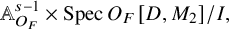 $$\begin{align*}\mathbb{A}_{O_F}^{s-1}\times \mathrm{Spec \, } O_F[D, M_2]/I, \end{align*}$$
where
 $$\begin{align*}I=(M_2'-[\mathbf{0}\mid I_{s-1}],\ D+D^t,\ D\cdot Q+2\pi I_{s-1}) \end{align*}$$
for some choice of $M^{\prime }_2$
.
$M^{\prime }_2$
. $[\mathbf {0}\mid I_{s-1}]$
is of size
$[\mathbf {0}\mid I_{s-1}]$
is of size $(s-1)\times s$
, with the first column
$(s-1)\times s$
, with the first column $0$
.
$0$
.
Proof. The proof is similar to the proof of Theorem 4.2. Consider $(M_2Z_2^t)^t=-J_{n-2}(M_2Z_2^t)J_{n-2}$
first. We claim that
$(M_2Z_2^t)^t=-J_{n-2}(M_2Z_2^t)J_{n-2}$
first. We claim that $Z_2^t$
depends on
$Z_2^t$
depends on $M_2$
and D. Since
$M_2$
and D. Since $M_2Z_2^t=(\sum _{k=2}^{s}a_{i,k}z_{j,k}')_{ij}$
, the relation
$M_2Z_2^t=(\sum _{k=2}^{s}a_{i,k}z_{j,k}')_{ij}$
, the relation $(M_2Z_2^t)^t=-J_{n-2}(M_2Z_2^t)J_{n-2}$
amounts to
$(M_2Z_2^t)^t=-J_{n-2}(M_2Z_2^t)J_{n-2}$
amounts to
 $$\begin{align*}a_{i,2}z_{j,2}'+\cdots+a_{i,s}z_{j,s}'=\pm(a_{n-1-j,2} z_{n-1-i,2}'+\cdots +a_{n-1-j,s}z_{n-1-i,s}'), \end{align*}$$
where the different sign $\pm $
depends on the position of
$\pm $
depends on the position of $i_2,\dots , i_s$
. We obtain
$i_2,\dots , i_s$
. We obtain
 $$\begin{align*}z_{n-1-i_2,2}'=z_{n-1-i_3,3}'=\dots =z_{n-1-i_s,s}'=0, \end{align*}$$
by letting $i=i_k$
,
$i=i_k$
, $j=n-1-i_k$
for
$j=n-1-i_k$
for $k=2,\dots ,s$
. To write down
$k=2,\dots ,s$
. To write down $Z_2^t$
explicitly, we need to consider the positions of
$Z_2^t$
explicitly, we need to consider the positions of $i_2,\dots ,i_s$
.
$i_2,\dots ,i_s$
.
Case 1: Assume that $1\leq i_2,\dots ,i_s\leq m-1$
. In this case, we have
$1\leq i_2,\dots ,i_s\leq m-1$
. In this case, we have $z_{n-1-i_p,q}'=-z_{n-1-i_q,p}'$
by letting
$z_{n-1-i_p,q}'=-z_{n-1-i_q,p}'$
by letting $i=i_{p}$
,
$i=i_{p}$
, $j=n-1-i_{q}$
. Set
$j=n-1-i_{q}$
. Set $d_{p,q}=z_{n-1-i_p,q}'$
. We obtain
$d_{p,q}=z_{n-1-i_p,q}'$
. We obtain
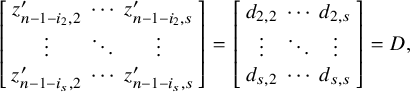 $$\begin{align*}\left[\begin{array}{ccc} z_{n-1-i_2,2}'& \cdots & z_{n-1-i_2,s}'\\ \vdots &\ddots & \vdots\\ z_{n-1-i_s,2}'& \cdots & z_{n-1-i_s,s}' \end{array}\right] = \left[\begin{array}{ccc} d_{2,2}&\cdots & d_{2,s}\\ \vdots &\ddots &\vdots\\ d_{s,2}&\cdots & d_{s,s} \end{array}\right]=D, \end{align*}$$
where $d_{p,q}=-d_{q,p}$
for
$d_{p,q}=-d_{q,p}$
for $2\leq p,q\leq s$
. This implies that D is skew-symmetric.
$2\leq p,q\leq s$
. This implies that D is skew-symmetric.
For $i=i_2$
, we have
$i=i_2$
, we have
 $$\begin{align*}z_{j,2}'=\pm(a_{n-1-j,2}d_{2,2}+\cdots +a_{n-1-j,s}d_{2,s}). \end{align*}$$
Since $1\leq i_2\leq m-1$
, the sign
$1\leq i_2\leq m-1$
, the sign $\pm $
is positive when
$\pm $
is positive when $1\leq j\leq m-1$
, and is negative when
$1\leq j\leq m-1$
, and is negative when $m\leq j\leq n-2$
. Similar to
$m\leq j\leq n-2$
. Similar to $i=i_k$
for
$i=i_k$
for $k=3,\dots , s$
. We have
$k=3,\dots , s$
. We have
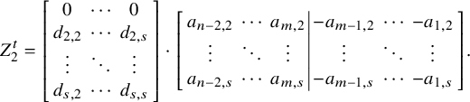 $$\begin{align*}Z_2^t= \left[\begin{array}{ccc} 0&\cdots &0\\ d_{2,2}&\cdots & d_{2,s}\\ \vdots &\ddots &\vdots\\ d_{s,2}&\cdots & d_{s,s} \end{array}\right]\cdot \left[\begin{array}{ccc|ccc} a_{n-2,2}&\cdots & a_{m,2} & -a_{m-1,2}&\cdots & -a_{1,2}\\ \vdots & \ddots & \vdots &\vdots &\ddots &\vdots\\ a_{n-2,s}&\cdots & a_{m,s} & -a_{m-1,s} & \cdots &-a_{1,s} \end{array} \right]. \end{align*}$$
Case 2: In general, we assume that
 $$\begin{align*}1\leq i_2,\dots, i_t\leq m-1 \quad \text{and} \quad m\leq i_{t+1},\dots, i_s\leq n-2. \end{align*}$$
Set $d_{p,q}=z_{n-1-i_p,q}'$
. By letting
$d_{p,q}=z_{n-1-i_p,q}'$
. By letting $i=i_p, j=n-1-i_q$
, we obtain
$i=i_p, j=n-1-i_q$
, we obtain
 $$\begin{align*}\begin{array}{l} d_{p,q}=-d_{q,p}, \quad \text{for}~ 2\leq p,q\leq t, ~\text{or}~ t+1\leq p,q\leq s,\\ d_{p,q}=d_{q,p}, \quad \text{for}~ 2\leq p\leq t, t+1\leq q\leq s, ~\text{or}~ t+1\leq p\leq s, 2\leq q\leq t. \end{array} \end{align*}$$
Thus, $z_{j,k}'=\pm (a_{n-1-j,k}d_{k,2}+\cdots +a_{n-1-j,s}d_{k,s})$
, where the sign
$z_{j,k}'=\pm (a_{n-1-j,k}d_{k,2}+\cdots +a_{n-1-j,s}d_{k,s})$
, where the sign $\pm $
is positive if
$\pm $
is positive if $1\leq j\leq m$
,
$1\leq j\leq m$
, $2\leq k\leq t$
, or
$2\leq k\leq t$
, or $m\leq j\leq n-2$
,
$m\leq j\leq n-2$
, $t+1\leq k\leq s$
, and negative otherwise. Therefore,
$t+1\leq k\leq s$
, and negative otherwise. Therefore, $Z_2^t$
can be expressed as
$Z_2^t$
can be expressed as
 $$\begin{align*}Z_2^t= \left[\begin{array}{ccc} 0&\cdots &0\\ d_{2,2}&\cdots & d_{2,s}\\ \vdots &\ddots &\vdots\\ d_{t,2}&\cdots & d_{t,s}\\ \hline -d_{t+1,2}&\cdots & -d_{t+1,s}\\ \vdots &\ddots &\vdots\\ -d_{s,2}&\cdots & -d_{s,s} \end{array}\right]\cdot \left[\begin{array}{ccc|ccc} a_{n-2,2}&\cdots & a_{m,2} & -a_{m-1,2}&\cdots & -a_{1,2}\\ \vdots &\ddots & \vdots &\vdots &\ddots &\vdots\\ a_{n-2,s}&\cdots & a_{m,s} & -a_{m-1,s} & \cdots &-a_{1,s} \end{array} \right]. \end{align*}$$
Set
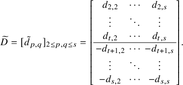 $$\begin{align*}\widetilde{D}=[\tilde{d}_{p,q}]_{2\leq p,q\leq s}=\left[\begin{array}{ccc} d_{2,2}&\cdots & d_{2,s}\\ \vdots &\ddots &\vdots\\ d_{t,2}&\cdots & d_{t,s}\\ \hline -d_{t+1,2}&\cdots & -d_{t+1,s}\\ \vdots &\ddots &\vdots\\ -d_{s,2}&\cdots & -d_{s,s} \end{array}\right]. \end{align*}$$
For $2\leq p,q\leq t$
, we have
$2\leq p,q\leq t$
, we have $\tilde {d}_{p,q}=d_{p,q}=-d_{q,p}=-\tilde {d}_{q,p}$
. Similarly, it is easy to see that
$\tilde {d}_{p,q}=d_{p,q}=-d_{q,p}=-\tilde {d}_{q,p}$
. Similarly, it is easy to see that $\tilde {d}_{p,q}=-\tilde {d}_{q,p}$
for all the other positions of
$\tilde {d}_{p,q}=-\tilde {d}_{q,p}$
for all the other positions of $p,q$
. Hence, the matrix
$p,q$
. Hence, the matrix $\widetilde {D}$
is skew-symmetric.
$\widetilde {D}$
is skew-symmetric.
Combining the above cases, for any $1\leq i_2,\dots , i_s\leq n-2$
, there exists a skew-symmetric matrix
$1\leq i_2,\dots , i_s\leq n-2$
, there exists a skew-symmetric matrix $\mathcal {D}$
of size
$\mathcal {D}$
of size $(s-1)\times (s-1)$
such that
$(s-1)\times (s-1)$
such that
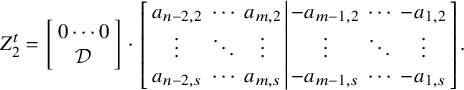 $$ \begin{align} Z_2^t= \left[\begin{array}{c}0\cdots 0\\ \mathcal{D}\end{array}\right]\cdot \left[\begin{array}{ccc|ccc} a_{n-2,2}&\cdots & a_{m,2} & -a_{m-1,2}&\cdots & -a_{1,2}\\ \vdots &\ddots & \vdots &\vdots &\ddots &\vdots\\ a_{n-2,s}&\cdots & a_{m,s} & -a_{m-1,s} & \cdots &-a_{1,s} \end{array} \right]. \end{align} $$
By abuse of notation, write $ D$
for
$ D$
for $ \mathcal {D}$
. Our next goal is to show that the second column of
$ \mathcal {D}$
. Our next goal is to show that the second column of $Z_1^t$
depends on the first column of
$Z_1^t$
depends on the first column of $Z_1^t$
and
$Z_1^t$
and $M_2$
. Recall that
$M_2$
. Recall that
 $$\begin{align*}C=\left[\begin{array}{cc} \mathbf{a_1}+z_{1,2}\mathbf{a_2}+\cdots +z_{1,s}\mathbf{a_s} & \pi \mathbf{a_1}+z_{2,2}\mathbf{a_2}+\cdots +z_{2,s}\mathbf{a_s} \end{array}\right] \end{align*}$$
and $B=J_2C^tJ_{n-2}$
. By using (4.2.1), the
$B=J_2C^tJ_{n-2}$
. By using (4.2.1), the $(n-1-i_k)$
-th columns (
$(n-1-i_k)$
-th columns ( $k=2,\dots , s$
) of the relation
$k=2,\dots , s$
) of the relation $B_1+\pi B_2=B_2(M_2Z_2^t)$
give
$B_1+\pi B_2=B_2(M_2Z_2^t)$
give
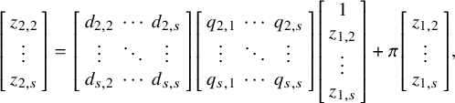 $$ \begin{align} \left[\begin{array}{c} z_{2,2}\\ \vdots\\ z_{2,s} \end{array}\right]=\left[\begin{array}{ccc} d_{2,2}&\cdots & d_{2,s}\\ \vdots &\ddots & \vdots\\ d_{s,2}&\cdots & d_{s,s} \end{array}\right] \left[\begin{array}{ccc} q_{2,1}&\cdots & q_{2,s}\\ \vdots &\ddots & \vdots\\ q_{s,1}&\cdots & q_{s,s} \end{array}\right] \left[\begin{array}{c} 1\\ z_{1,2}\\ \vdots\\ z_{1,s} \end{array}\right]+\pi \left[\begin{array}{c} z_{1,2}\\ \vdots\\ z_{1,s} \end{array}\right], \end{align} $$
where $q_{i,j}=\sum _{k=1}^{m-1}(a_{k,i}a_{n-1-k.j}-a_{n-1-k,i}a_{k,j})$
. It is easy to see that the rest columns in
$q_{i,j}=\sum _{k=1}^{m-1}(a_{k,i}a_{n-1-k.j}-a_{n-1-k,i}a_{k,j})$
. It is easy to see that the rest columns in $B_1+\pi B_2= B_2(M_2Z_2^t)$
are automatically satisfied when (4.2.2) holds.
$B_1+\pi B_2= B_2(M_2Z_2^t)$
are automatically satisfied when (4.2.2) holds.
Finally, consider $CM_1+(M_2Z_2^t)M_2=2\pi M_2$
. By using the relations (4.2.1) and (4.2.2), it is equivalent to
$CM_1+(M_2Z_2^t)M_2=2\pi M_2$
. By using the relations (4.2.1) and (4.2.2), it is equivalent to
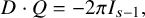 $$\begin{align*}D\cdot Q=-2\pi I_{s-1}, \end{align*}$$
where
 $$\begin{align*}D=\left[\begin{array}{ccc} d_{2,2}&\cdots & d_{2,s}\\ \vdots &\ddots &\vdots\\ d_{s,2}&\cdots & d_{s,s} \end{array}\right],\quad Q=\left[\begin{array}{ccc} q_{2,2}&\cdots & q_{2,s}\\ \vdots &\ddots &\vdots\\ q_{s,2}&\cdots & q_{s,s} \end{array}\right]. \end{align*}$$
There are two relations we still need to consider: $B_1M_2=\pi B_2M_2$
, and
$B_1M_2=\pi B_2M_2$
, and $(M_2Z_2^t)^2=2\pi (M_2Z_2^t)$
. We leave it to the reader to verify that these conditions are already satisfied when
$(M_2Z_2^t)^2=2\pi (M_2Z_2^t)$
. We leave it to the reader to verify that these conditions are already satisfied when $D\cdot Q=-2\pi I_{s-1}$
.
$D\cdot Q=-2\pi I_{s-1}$
.
From all the above, we deduce that an affine neighborhood around $(\mathcal {F}_0,\Lambda ')$
is given by
$(\mathcal {F}_0,\Lambda ')$
is given by $ _2\mathcal {U}_{r,s}\cong \mathrm {Spec \, } O_F[x,z_{1,2},\dots ,z_{1,s}, D, M_2]/I$
, where
$ _2\mathcal {U}_{r,s}\cong \mathrm {Spec \, } O_F[x,z_{1,2},\dots ,z_{1,s}, D, M_2]/I$
, where
 $$\begin{align*}I=(M_2'-[\mathbf{0}\mid I_{s-1}],\ D+D^t,\ D\cdot Q+2\pi I_{s-1}). \end{align*}$$
Set $\mathbb {A}_{O_F}^{s-1}=\mathrm {Spec \, } O_F[x,z_{1,2},\dots ,z_{1,s}]$
. For
$\mathbb {A}_{O_F}^{s-1}=\mathrm {Spec \, } O_F[x,z_{1,2},\dots ,z_{1,s}]$
. For $s\geq 2$
, we have
$s\geq 2$
, we have
 $$\begin{align*}_2{\mathcal U}_{r,s}\cong \mathbb{A}_{O_F}^{s-1}\times \mathrm{Spec \, } O_F [D,M_2]/I.\\[-41pt] \end{align*}$$
In particular, for the signature $(r,s)=(n-3,3)$
, we have
$(r,s)=(n-3,3)$
, we have
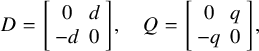 $$\begin{align*}D=\left[\begin{array}{cc} 0 & d\\ -d& 0 \end{array}\right],\quad Q=\left[\begin{array}{cc} 0 & q\\ -q& 0 \end{array}\right], \end{align*}$$
where we set $d=d_{2,3}=-d_{3,2}, q=q_{2,3}=-q_{3,2}$
. Recall that
$d=d_{2,3}=-d_{3,2}, q=q_{2,3}=-q_{3,2}$
. Recall that $q=\sum _{k=1}^{m-1}(a_{k,2}a_{n-1-k,3}-a_{n-1-k,2}a_{k,3})$
. The equation
$q=\sum _{k=1}^{m-1}(a_{k,2}a_{n-1-k,3}-a_{n-1-k,2}a_{k,3})$
. The equation $D\cdot Q=-2\pi I_{s-1}$
amounts to
$D\cdot Q=-2\pi I_{s-1}$
amounts to $d\cdot q-2\pi =0$
.
$d\cdot q-2\pi =0$
.
Corollary 4.9. When $(r,s)=(n-3,3)$
, there is an affine chart
$(r,s)=(n-3,3)$
, there is an affine chart $_2{\mathcal U}_{n-3,3}$
which is isomorphic to
$_2{\mathcal U}_{n-3,3}$
which is isomorphic to
 $$\begin{align*}V(I)=\mathrm{Spec \, } O_F[x,z_{1,2}, z_{1,3}, d, (a_{k,1})_{1\leq k\leq n-2}, (a_{k,2})_{1\leq k\leq n-2}, (a_{k,3})_{1\leq k\leq n-2}]/I, \end{align*}$$
where
 $$\begin{align*}I=(a_{i_2,1}, a_{i_3,1}, a_{i_2,2}-1, a_{i_3,2}, a_{i_2,3}, a_{i_3,3}-1, d\cdot \sum_{k=1}^{m-1}(a_{k,2}a_{n-1-k,3}-a_{n-1-k,2}a_{k,3})-2\pi) \end{align*}$$
for some $ 1 \leq i_2,i_3 \leq n-2$
.
$ 1 \leq i_2,i_3 \leq n-2$
.
Remark 4.10. As in Remark 4.4, for different choices of $M^{\prime }_2$
, we get different equations from
$M^{\prime }_2$
, we get different equations from $D\cdot Q = -2 \pi I_s$
and so different affine charts
$D\cdot Q = -2 \pi I_s$
and so different affine charts $_2\mathcal {U}_{r,s}$
which in general are not isomorphic. For instance, in Corollary 4.9, there are two different affine charts up to isomorphism when we choose different positions for
$_2\mathcal {U}_{r,s}$
which in general are not isomorphic. For instance, in Corollary 4.9, there are two different affine charts up to isomorphism when we choose different positions for $i_2, i_3$
(see §5.3 for details). In Proposition 5.7, we show that for any such a choice, the affine scheme
$i_2, i_3$
(see §5.3 for details). In Proposition 5.7, we show that for any such a choice, the affine scheme $V (I)$
has semi-stable reduction over
$V (I)$
has semi-stable reduction over $O_F$
.
$O_F$
.
5 Splitting models
$\mathrm {M}^{\mathrm {spl}}$

In this section, we will first show that the naive splitting model $\mathcal {M}$
is not flat over
$\mathcal {M}$
is not flat over $\mathrm {Spec \, } O_F$
for a general signature
$\mathrm {Spec \, } O_F$
for a general signature $(r,s)$
. Then we will define the closed subscheme
$(r,s)$
. Then we will define the closed subscheme $\mathrm {M}^{\mathrm {spl}} \subset \mathcal {M} $
. We show that
$\mathrm {M}^{\mathrm {spl}} \subset \mathcal {M} $
. We show that $\mathrm {M}^{\mathrm {spl}}$
is smooth for the signature
$\mathrm {M}^{\mathrm {spl}}$
is smooth for the signature $(r,s)=(n-1,1)$
and has semi-stable reduction for the signature
$(r,s)=(n-1,1)$
and has semi-stable reduction for the signature $(r,s)=(n-2,2)$
and
$(r,s)=(n-2,2)$
and $(r,s)=(n-3,3)$
.
$(r,s)=(n-3,3)$
.
5.1 Naive Splitting Models
$\mathcal {M}$

By using the explicit description of the two affine charts $_1{\mathcal U}_{r,s}$
,
$_1{\mathcal U}_{r,s}$
, $_2{\mathcal U}_{r,s}\subset \mathcal {M}$
, that we obtained in §4, we will show that
$_2{\mathcal U}_{r,s}\subset \mathcal {M}$
, that we obtained in §4, we will show that $\mathcal {M}$
is not flat over
$\mathcal {M}$
is not flat over $\mathrm {Spec \, } O_F$
.
$\mathrm {Spec \, } O_F$
.
Proposition 5.1. For any signature $(r,s)$
, the naive splitting model
$(r,s)$
, the naive splitting model $\mathcal {M}$
is not flat over
$\mathcal {M}$
is not flat over $\mathrm {Spec \, } O_F$
.
$\mathrm {Spec \, } O_F$
.
Proof. It is enough to show a) When s is odd, the generic fiber $_1{\mathcal U}_{r,s}\otimes _{O_F}F$
is empty and so the point
$_1{\mathcal U}_{r,s}\otimes _{O_F}F$
is empty and so the point $(\mathcal {F}_0, t\Lambda _m)$
does not lift to characteristic zero, and b) When s is even, the generic fiber
$(\mathcal {F}_0, t\Lambda _m)$
does not lift to characteristic zero, and b) When s is even, the generic fiber $_2{\mathcal U}_{r,s}\otimes _{O_F}F$
is empty and so the point
$_2{\mathcal U}_{r,s}\otimes _{O_F}F$
is empty and so the point $(\mathcal {F}_0, \Lambda ')$
does not lift to characteristic zero.
$(\mathcal {F}_0, \Lambda ')$
does not lift to characteristic zero.
Observe that for a skew-symmetric matrix P of size $s\times s$
, the determinant of P is equal to
$s\times s$
, the determinant of P is equal to $0$
if s is odd. Recall that we denote by
$0$
if s is odd. Recall that we denote by $_1{\mathcal U}_{r,s}$
the affine chart around the point
$_1{\mathcal U}_{r,s}$
the affine chart around the point $(\mathcal {F}_0, t\Lambda _m)\in \mathcal {M}$
. By Theorem 4.2, the affine chart
$(\mathcal {F}_0, t\Lambda _m)\in \mathcal {M}$
. By Theorem 4.2, the affine chart $_1{\mathcal U}_{r,s}$
is isomorphic to
$_1{\mathcal U}_{r,s}$
is isomorphic to $\mathrm {Spec \, } O_F[D,Y]/I$
, where
$\mathrm {Spec \, } O_F[D,Y]/I$
, where
 $$\begin{align*}I=(Y'-I_s, \ D+D^t, \ D\cdot Q+2\pi I_s), \end{align*}$$
for any signature $(r,s)$
. Here, D is a skew-symmetric matrix of size
$(r,s)$
. Here, D is a skew-symmetric matrix of size $s\times s$
. Thus, when s is odd, we have
$s\times s$
. Thus, when s is odd, we have $\det (D)=0$
. In this case, we can see that the generic fiber
$\det (D)=0$
. In this case, we can see that the generic fiber $_1{\mathcal U}_{r,s}\otimes _{O_F}F$
is empty since
$_1{\mathcal U}_{r,s}\otimes _{O_F}F$
is empty since
 $$\begin{align*}0=\det(D)\det(Q)=\det(D\cdot Q)=\det(-2\pi I_s)=(-2\pi)^s. \end{align*}$$
It follows that the point $(\mathcal {F}_0, t\Lambda _m)$
does not lift to characteristic zero when s is odd.
$(\mathcal {F}_0, t\Lambda _m)$
does not lift to characteristic zero when s is odd.
Recall that we denote by $_2{\mathcal U}_{r,s}$
the affine chart around the point
$_2{\mathcal U}_{r,s}$
the affine chart around the point $(\mathcal {F}_0, \Lambda ')\in \mathcal {M}$
. By Theorem 4.8, the affine chart
$(\mathcal {F}_0, \Lambda ')\in \mathcal {M}$
. By Theorem 4.8, the affine chart $_2{\mathcal U}_{r,s}$
is isomorphic to
$_2{\mathcal U}_{r,s}$
is isomorphic to $\mathbb {A}^{s-1}_{O_F}\times \mathrm {Spec \, } O_F[D,M_2]/I$
, where
$\mathbb {A}^{s-1}_{O_F}\times \mathrm {Spec \, } O_F[D,M_2]/I$
, where
 $$\begin{align*}I=(M_2'-[0\mid I_s], \ D+D^t, \ D\cdot Q+2\pi I_{s-1}). \end{align*}$$
When s is even, we see that the generic fiber $_2{\mathcal U}_{r,s}\otimes _{O_F}F$
is empty since D is of size
$_2{\mathcal U}_{r,s}\otimes _{O_F}F$
is empty since D is of size $(s-1)\times (s-1)$
and
$(s-1)\times (s-1)$
and $0=\det (D\cdot Q)=(-2\pi )^{s-1}$
. Therefore, the point
$0=\det (D\cdot Q)=(-2\pi )^{s-1}$
. Therefore, the point $(\mathcal {F}_0, \Lambda ')$
does not lift to characteristic zero when s is even.
$(\mathcal {F}_0, \Lambda ')$
does not lift to characteristic zero when s is even.
Recall that there is a forgetful morphism $\tau : \mathcal {M}\rightarrow \mathrm {M}^\wedge \otimes _O O_F$
. From [Reference Pappas and Rapoport18, Remark 5.3], [Reference Pappas, Rapoport and Smithling20, Remark 2.6.10], the authors show that the wedge local model
$\tau : \mathcal {M}\rightarrow \mathrm {M}^\wedge \otimes _O O_F$
. From [Reference Pappas and Rapoport18, Remark 5.3], [Reference Pappas, Rapoport and Smithling20, Remark 2.6.10], the authors show that the wedge local model $\mathrm {M}^\wedge $
is not topological flat for any signature when n is even. Consider the local model
$\mathrm {M}^\wedge $
is not topological flat for any signature when n is even. Consider the local model $\mathrm {M}^{\mathrm {loc}}$
to be the scheme-theoretic closure in
$\mathrm {M}^{\mathrm {loc}}$
to be the scheme-theoretic closure in $\mathrm {M}^\wedge $
of its generic fiber. We have a closed morphism
$\mathrm {M}^\wedge $
of its generic fiber. We have a closed morphism $\mathrm {M}^{\mathrm {loc}}\hookrightarrow \mathrm {M}^\wedge $
. Define the splitting model as the inverse image of
$\mathrm {M}^{\mathrm {loc}}\hookrightarrow \mathrm {M}^\wedge $
. Define the splitting model as the inverse image of $\mathrm {M}^{\mathrm {loc}}$
; that is,
$\mathrm {M}^{\mathrm {loc}}$
; that is,
 $$\begin{align*}\mathrm{M}^{\mathrm{spl}}:=\tau^{-1}(\mathrm{M}^{\mathrm{loc}})=\mathcal{M}\times_{\mathrm{M}^\wedge} \mathrm{M}^{\mathrm{loc}}. \end{align*}$$
The restriction of the forgetful morphism $\tau $
on
$\tau $
on $\mathrm {M}^{\mathrm {spl}}$
gives
$\mathrm {M}^{\mathrm {spl}}$
gives
 $$\begin{align*}\tau: \mathrm{M}^{\mathrm{spl}}\rightarrow \mathrm{M}^{\mathrm{loc}}. \end{align*}$$
5.2 The Case
$(r,s)=(n-2,2)$

By using the explicit description of $ _1\mathcal {U}_{n-2,2}$
in §4.1, we show the following.
$ _1\mathcal {U}_{n-2,2}$
in §4.1, we show the following.
Proposition 5.2. When $(r,s)=(n-2,2)$
,
$(r,s)=(n-2,2)$
, $_1{\mathcal U}_{n-2,2}$
has semi-stable reduction over
$_1{\mathcal U}_{n-2,2}$
has semi-stable reduction over $O_F$
. In particular,
$O_F$
. In particular, $_1{\mathcal U}_{n-2,2}$
is regular and has special fiber a reduced divisor with two smooth irreducible components intersecting transversely.
$_1{\mathcal U}_{n-2,2}$
is regular and has special fiber a reduced divisor with two smooth irreducible components intersecting transversely.
Proof. From Corollary 4.3, it is enough to show that the scheme $V(I) $
has semi-stable reduction over
$V(I) $
has semi-stable reduction over $O_F$
. It suffices to prove that
$O_F$
. It suffices to prove that $V(I) $
is regular and its special fiber is reduced with smooth irreducible components that have smooth intersections with correct dimensions (see [Reference de Jong13, §2.16]).
$V(I) $
is regular and its special fiber is reduced with smooth irreducible components that have smooth intersections with correct dimensions (see [Reference de Jong13, §2.16]).
First, we rename our variables as follows: $x_i := y_{i,1}$
and
$x_i := y_{i,1}$
and $y_i := y_{i,2}$
for
$y_i := y_{i,2}$
for $1 \leq i \leq n.$
Thus,
$1 \leq i \leq n.$
Thus, $V(I) = \mathrm {Spec \, } O_F[d,\underline x, \underline y]/ I$
, where
$V(I) = \mathrm {Spec \, } O_F[d,\underline x, \underline y]/ I$
, where
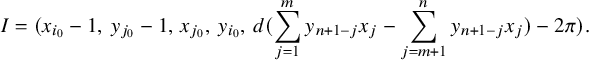 $$\begin{align*}I= ( x_{i_0}-1,\, y_{j_0} -1 ,\,x_{j_0},\,y_{i_0},\, d(\sum^m_{j=1}y_{n+1-j}x_{j} - \sum^n_{j=m+1}y_{n+1-j}x_{j}) -2 \pi). \end{align*}$$
By symmetry, as above, there two cases to consider: Case 1 when $1 \leq i_0,\,j_0 \leq m$
and Case 2 when
$1 \leq i_0,\,j_0 \leq m$
and Case 2 when $ 1 \leq i_0 \leq m$
and
$ 1 \leq i_0 \leq m$
and $ m+1 \leq j_0 \leq n $
. We consider these two cases separately in this proof.
$ m+1 \leq j_0 \leq n $
. We consider these two cases separately in this proof.
In Case 1, we can assume, for simplicity, that $i_0=1$
and
$i_0=1$
and $ j_0=2$
. Thus,
$ j_0=2$
. Thus, $V(I)$
is isomorphic to
$V(I)$
is isomorphic to $V(\mathcal {I}) = \mathrm {Spec \, } R/\mathcal {I}$
, where
$V(\mathcal {I}) = \mathrm {Spec \, } R/\mathcal {I}$
, where
 $$\begin{align*}R = O_F[d,(x_i)_{3\leq i \leq n}, (y_i)_{3\leq i \leq n}], \end{align*}$$
and
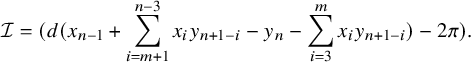 $$\begin{align*}\mathcal{I} = (d(x_{n-1} +\sum^{n-3}_{i=m+1}x_iy_{n+1-i}- y_n - \sum^m_{i=3}x_iy_{n+1-i}) -2\pi ). \end{align*}$$
Over the special fiber ( $\pi =0$
), we have
$\pi =0$
), we have $ V(\mathcal {I} _s) \cong \mathrm {Spec \, } \bar {R}/\mathcal {I}_s $
, where
$ V(\mathcal {I} _s) \cong \mathrm {Spec \, } \bar {R}/\mathcal {I}_s $
, where
 $$\begin{align*}\bar{R} = k[d,(x_i)_{3\leq i \leq n}, (y_i)_{3\leq i \leq n}], \quad \mathcal{I}_s= (d(x_{n-1} +\sum^{n-3}_{i=m+1}x_iy_{n+1-i}- y_n - \sum^m_{i=3}x_iy_{n+1-i}) ). \end{align*}$$
It has two smooth irreducible components $V(\mathcal {I}_i) = \mathrm {Spec \, } \bar {R}/\mathcal {I}_i$
, where
$V(\mathcal {I}_i) = \mathrm {Spec \, } \bar {R}/\mathcal {I}_i$
, where
 $$\begin{align*}\mathcal{I}_1 = (d), \quad \mathcal{I}_2 = (x_{n-1} +\sum^{n-3}_{i=m+1}x_iy_{n+1-i}- y_n - \sum^m_{i=3}x_iy_{n+1-i}), \end{align*}$$
that are isomorphic to $\mathbb {A}_k^{2n-4}$
. Their intersection is also smooth and of dimension
$\mathbb {A}_k^{2n-4}$
. Their intersection is also smooth and of dimension $2n-5$
. Next, we prove that
$2n-5$
. Next, we prove that $V(\mathcal {I} _s)$
is reduced by showing that
$V(\mathcal {I} _s)$
is reduced by showing that $\mathcal {I}_s =\mathcal {I}_1 \cap \mathcal {I}_2.$
Clearly,
$\mathcal {I}_s =\mathcal {I}_1 \cap \mathcal {I}_2.$
Clearly, $\mathcal {I} _s \subset \mathcal {I}_1 \cap \mathcal {I}_2$
. Let
$\mathcal {I} _s \subset \mathcal {I}_1 \cap \mathcal {I}_2$
. Let $g \in \mathcal {I}_1 \cap \mathcal {I}_2 .$
Thus,
$g \in \mathcal {I}_1 \cap \mathcal {I}_2 .$
Thus, $g \in \mathcal {I}_1$
and
$g \in \mathcal {I}_1$
and $g = f_1 d$
for
$g = f_1 d$
for $f_1 \in \bar {R}$
. Also,
$f_1 \in \bar {R}$
. Also, $g \in \mathcal {I}_2$
and so
$g \in \mathcal {I}_2$
and so $f_1 d \in \mathcal {I}_2$
.
$f_1 d \in \mathcal {I}_2$
. $\mathcal {I}_2$
is a prime ideal and
$\mathcal {I}_2$
is a prime ideal and $d \notin \mathcal {I}_2$
. Thus,
$d \notin \mathcal {I}_2$
. Thus, $f_1 \in \mathcal {I}_2$
and
$f_1 \in \mathcal {I}_2$
and
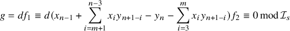 $$\begin{align*}g = df_1 \equiv d (x_{n-1} +\sum^{n-3}_{i=m+1}x_iy_{n+1-i}- y_n - \sum^m_{i=3}x_iy_{n+1-i}) f_2 \equiv 0 \, \text{mod} \, \mathcal{I}_s \end{align*}$$
for $f_2 \in \bar {R}$
. Thus,
$f_2 \in \bar {R}$
. Thus, $g \in \mathcal {I}_s$
and so
$g \in \mathcal {I}_s$
and so $\mathcal {I}_s = \mathcal {I}_1 \cap \mathcal {I}_2 .$
Lastly, we can easily see that the ideals
$\mathcal {I}_s = \mathcal {I}_1 \cap \mathcal {I}_2 .$
Lastly, we can easily see that the ideals $ \mathcal {I}_1,\mathcal {I}_2$
are principal over
$ \mathcal {I}_1,\mathcal {I}_2$
are principal over $V(\mathcal {I})$
. From the above, we deduce that
$V(\mathcal {I})$
. From the above, we deduce that $V(\mathcal {I}) $
is regular (see [Reference Hartl10, Remark 1.1.1]).
$V(\mathcal {I}) $
is regular (see [Reference Hartl10, Remark 1.1.1]).
In Case 2, we set $\Delta =\{1,\dots ,n-2\}/ \{m, m+1\}$
and let
$\Delta =\{1,\dots ,n-2\}/ \{m, m+1\}$
and let $i_0=m, j_0=m+1$
. Then
$i_0=m, j_0=m+1$
. Then $V(I)$
is isomorphic to
$V(I)$
is isomorphic to $V(\mathcal {J}) = \mathrm {Spec \, } R'/\mathcal {J}$
, where
$V(\mathcal {J}) = \mathrm {Spec \, } R'/\mathcal {J}$
, where $R' = O_F[d,(x_i)_{i \in \Delta }, (y_i)_{i \in \Delta }]$
and
$R' = O_F[d,(x_i)_{i \in \Delta }, (y_i)_{i \in \Delta }]$
and
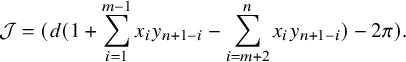 $$\begin{align*}\mathcal{J} = (d(1+ \sum^{m-1}_{i=1}x_iy_{n+1-i}- \sum^n_{i= m+2}x_iy_{n+1-i})-2\pi). \end{align*}$$
To see that $V(\mathcal {J}) $
has semi-stable reduction over
$V(\mathcal {J}) $
has semi-stable reduction over $O_F$
, one proceeds exactly as in Case 1. Over the special fiber (
$O_F$
, one proceeds exactly as in Case 1. Over the special fiber ( $\pi =0$
), we have
$\pi =0$
), we have $ V(\mathcal {J} _s) \cong \mathrm {Spec \, } \bar {R}'/\mathcal {J}_s $
where
$ V(\mathcal {J} _s) \cong \mathrm {Spec \, } \bar {R}'/\mathcal {J}_s $
where $ \bar {R} = k[d,(x_i)_{i \in \Delta }, (y_i)_{i \in \Delta }]$
and
$ \bar {R} = k[d,(x_i)_{i \in \Delta }, (y_i)_{i \in \Delta }]$
and
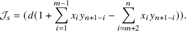 $$\begin{align*}\mathcal{J}_s = (d(1+ \sum^{m-1}_{i=1}x_iy_{n+1-i}- \sum^n_{i= m+2}x_iy_{n+1-i})). \end{align*}$$
It has two smooth irreducible components $V(\mathcal {J}_i) = \mathrm {Spec \, } R/\mathcal {J}_i$
, where
$V(\mathcal {J}_i) = \mathrm {Spec \, } R/\mathcal {J}_i$
, where
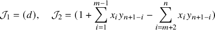 $$\begin{align*}\mathcal{J}_1 = (d), \quad \mathcal{J}_2 = (1+ \sum^{m-1}_{i=1}x_iy_{n+1-i}- \sum^n_{i= m+2}x_iy_{n+1-i}) \end{align*}$$
of dimension $2n-4$
. (Note that in this case, the second component
$2n-4$
. (Note that in this case, the second component $V(\mathcal {J}_2)$
is not isomorphic to the affine space
$V(\mathcal {J}_2)$
is not isomorphic to the affine space $\mathbb {A}_k^{2n-4}$
as in Case 1.) Their intersection is also smooth and of dimension
$\mathbb {A}_k^{2n-4}$
as in Case 1.) Their intersection is also smooth and of dimension $2n-5$
. By using similar arguments as Case 1, we can show that
$2n-5$
. By using similar arguments as Case 1, we can show that $V(\mathcal {J}_s)$
is reduced and
$V(\mathcal {J}_s)$
is reduced and $V(\mathcal {J})$
is regular.
$V(\mathcal {J})$
is regular.
Since $_1{\mathcal U}_{n-2,2}$
has semi-stable reduction, and is therefore flat over
$_1{\mathcal U}_{n-2,2}$
has semi-stable reduction, and is therefore flat over $O_F$
, we have
$O_F$
, we have $_1{\mathcal U}_{n-2,2}\subset \mathrm {M}^{\mathrm {spl}}$
. Our next goal is to prove that
$_1{\mathcal U}_{n-2,2}\subset \mathrm {M}^{\mathrm {spl}}$
. Our next goal is to prove that $\mathrm { M}^{\mathrm {spl}}$
has semi-stable reduction over
$\mathrm { M}^{\mathrm {spl}}$
has semi-stable reduction over $O_F$
for the signature
$O_F$
for the signature $(r,s)= (n-2,2)$
. From §4.1, it is enough to show that
$(r,s)= (n-2,2)$
. From §4.1, it is enough to show that $\mathcal {G}$
-translates of
$\mathcal {G}$
-translates of $_1{\mathcal U}_{n-2,2}$
cover
$_1{\mathcal U}_{n-2,2}$
cover $\mathrm {M}^{\mathrm {spl}}$
(see Theorem 5.4).
$\mathrm {M}^{\mathrm {spl}}$
(see Theorem 5.4).
Assume that s is even. Recall from §4.1 the ${\mathcal G}$
-equivariant morphism
${\mathcal G}$
-equivariant morphism $\tau : \mathrm {M}^{\mathrm {spl}} \rightarrow \mathrm {M}^{\mathrm {loc}}\otimes _{O} O_F$
which is given by
$\tau : \mathrm {M}^{\mathrm {spl}} \rightarrow \mathrm {M}^{\mathrm {loc}}\otimes _{O} O_F$
which is given by $(\mathcal {F}_0,\mathcal {F}_1) \mapsto \mathcal {F}_1$
. Let
$(\mathcal {F}_0,\mathcal {F}_1) \mapsto \mathcal {F}_1$
. Let $\tau _s : \mathrm {M}^{\mathrm {spl}}\otimes k \rightarrow \mathrm {M}^{\mathrm {loc}}\otimes k$
be the morphism over the special fiber. Let
$\tau _s : \mathrm {M}^{\mathrm {spl}}\otimes k \rightarrow \mathrm {M}^{\mathrm {loc}}\otimes k$
be the morphism over the special fiber. Let $(\mathcal {F}_0,\mathcal {F}_1)$
be point of the special fiber of
$(\mathcal {F}_0,\mathcal {F}_1)$
be point of the special fiber of $\mathrm {M}^{\mathrm {spl}}$
. Over the special fiber the condition (4) amounts to
$\mathrm {M}^{\mathrm {spl}}$
. Over the special fiber the condition (4) amounts to $t\mathcal {F}_0 = (0)$
and so
$t\mathcal {F}_0 = (0)$
and so $ (0) \subset \mathcal {F}_0 \subset t \Lambda _m \otimes k$
(see §3 for the definition of the naive splitting models). Hence, we consider the morphism
$ (0) \subset \mathcal {F}_0 \subset t \Lambda _m \otimes k$
(see §3 for the definition of the naive splitting models). Hence, we consider the morphism
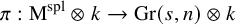 $$\begin{align*}\pi : \mathrm{M}^{\mathrm{spl}}\otimes k \rightarrow \mathrm{Gr}(s,n)\otimes k \end{align*}$$
given by $ (\mathcal {F}_0,\mathcal {F}_1) \mapsto \mathcal {F}_0.$
Here,
$ (\mathcal {F}_0,\mathcal {F}_1) \mapsto \mathcal {F}_0.$
Here, $\mathrm {Gr}(s,n)\otimes k$
is the finite-dimensional Grassmannian of s-dimensional subspaces of
$\mathrm {Gr}(s,n)\otimes k$
is the finite-dimensional Grassmannian of s-dimensional subspaces of $t \Lambda _m \otimes k.$
This has a section
$t \Lambda _m \otimes k.$
This has a section
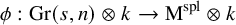 $$\begin{align*}\phi : \mathrm{Gr}(s,n)\otimes k \rightarrow \mathrm{M}^{\mathrm{spl}}\otimes k \end{align*}$$
given by $ \mathcal {F}_0 \mapsto (\mathcal {F}_0,\mathcal {F}_1)$
with
$ \mathcal {F}_0 \mapsto (\mathcal {F}_0,\mathcal {F}_1)$
with $\mathcal {F}_1 = t\Lambda _m \otimes k.$
The image of the section
$\mathcal {F}_1 = t\Lambda _m \otimes k.$
The image of the section $\phi $
is an irreducible component of
$\phi $
is an irreducible component of $ \mathrm {M}^{\mathrm { spl}}\otimes _{O_F} k$
which is the fiber
$ \mathrm {M}^{\mathrm { spl}}\otimes _{O_F} k$
which is the fiber $\tau ^{-1}_s (t\Lambda _m\otimes k)$
over the ‘worst point’ of
$\tau ^{-1}_s (t\Lambda _m\otimes k)$
over the ‘worst point’ of $\mathrm {M}^{\mathrm {loc}}\otimes k$
– that is, the unique closed
$\mathrm {M}^{\mathrm {loc}}\otimes k$
– that is, the unique closed ${\mathcal G}$
-orbit supported in the special fiber (see [Reference Pappas and Rapoport19, §5]). Hence,
${\mathcal G}$
-orbit supported in the special fiber (see [Reference Pappas and Rapoport19, §5]). Hence, $\tau ^{-1}_s(t\Lambda _m)$
is isomorphic to the Grassmannian
$\tau ^{-1}_s(t\Lambda _m)$
is isomorphic to the Grassmannian $ \mathrm {Gr}(s,n)\otimes k $
of dimension
$ \mathrm {Gr}(s,n)\otimes k $
of dimension $s(n-s)$
.
$s(n-s)$
.
We equip $t \Lambda _m \otimes k$
with the nondegenerate alternating form
$t \Lambda _m \otimes k$
with the nondegenerate alternating form $ \langle \, , \, \rangle '$
which is defined as
$ \langle \, , \, \rangle '$
which is defined as $\langle tv,tw \rangle ' := ( v,tw ) = v^tJ_n w$
. Note that this is well defined (see [Reference Richarz25, §5.2] for more details). Denote by
$\langle tv,tw \rangle ' := ( v,tw ) = v^tJ_n w$
. Note that this is well defined (see [Reference Richarz25, §5.2] for more details). Denote by $\mathcal {Q}(s,n)$
the closed subscheme of
$\mathcal {Q}(s,n)$
the closed subscheme of $\phi (\mathrm {Gr}(s,n)\otimes k) $
of dimension
$\phi (\mathrm {Gr}(s,n)\otimes k) $
of dimension $ s(2n-3s+1)/2$
which parametrizes all the isotropic s-subspaces
$ s(2n-3s+1)/2$
which parametrizes all the isotropic s-subspaces $\mathcal {F}_0$
in the n-space
$\mathcal {F}_0$
in the n-space $t\Lambda _m \otimes k$
.
$t\Lambda _m \otimes k$
.
Next, we give a couple of useful observations concerning the special fiber of the affine chart $_1{\mathcal U}_{r,s}$
(see §4.1 for the notation), which will be used in the proof of the following theorem.
$_1{\mathcal U}_{r,s}$
(see §4.1 for the notation), which will be used in the proof of the following theorem.
Remark 5.3. Recall from Theorem 4.2 that over the special fiber of $_1{\mathcal U}_{r,s}$
, we have
$_1{\mathcal U}_{r,s}$
, we have $D=-D^t$
,
$D=-D^t$
, $D\cdot Q=0$
and the minor relations from (4.1.1).
$D\cdot Q=0$
and the minor relations from (4.1.1).
a) Observe that if $D =0$
, then
$D =0$
, then $Z=0$
, which gives
$Z=0$
, which gives $A=0$
since
$A=0$
since $A = Y Z^t$
over the special fiber. If
$A = Y Z^t$
over the special fiber. If $A=0$
, then
$A=0$
, then $\mathcal {F}_1 = t \Lambda _m$
. Hence,
$\mathcal {F}_1 = t \Lambda _m$
. Hence, $_1{\mathcal U}_{r,s} \cap \tau ^{-1}(t\Lambda _m)$
is a smooth irreducible component of dimension
$_1{\mathcal U}_{r,s} \cap \tau ^{-1}(t\Lambda _m)$
is a smooth irreducible component of dimension $s(n-s)$
.
$s(n-s)$
.
b) Recall that
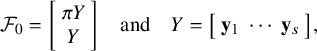 $$\begin{align*}\mathcal{F}_0= \left[\begin{array}{c} \pi Y \\ Y \end{array}\right] \quad \text{and} \quad Y = \left[\begin{array}{ccc} \mathbf{y}_1 \ \cdots \ \mathbf{y}_s \end{array}\right], \end{align*}$$
where $ \mathbf {y}_i$
are the columns of the matrix
$ \mathbf {y}_i$
are the columns of the matrix $Y.$
By direct calculations, we get that the entries
$Y.$
By direct calculations, we get that the entries $q_{i,j}$
of the matrix Q are given by
$q_{i,j}$
of the matrix Q are given by $q_{i,j} = \langle \mathbf {y}_i,\mathbf {y}_j \rangle '$
. Thus, over the special fiber, we have
$q_{i,j} = \langle \mathbf {y}_i,\mathbf {y}_j \rangle '$
. Thus, over the special fiber, we have $\langle \mathcal {F}_0,\mathcal {F}_0 \rangle ' = Q $
, and so from the rank of
$\langle \mathcal {F}_0,\mathcal {F}_0 \rangle ' = Q $
, and so from the rank of $ Q$
, we read how isotropic
$ Q$
, we read how isotropic $\mathcal {F}_0$
is with respect to
$\mathcal {F}_0$
is with respect to $\langle \,,\,\rangle '$
. When the rank of the matrix Q is zero, which actually occurs, we have
$\langle \,,\,\rangle '$
. When the rank of the matrix Q is zero, which actually occurs, we have $\langle \mathcal {F}_0,\mathcal {F}_0 \rangle ' = 0 $
.
$\langle \mathcal {F}_0,\mathcal {F}_0 \rangle ' = 0 $
.
c) From (a) and (b), we can easily see that $_1{\mathcal U}_{r,s}$
contains points
$_1{\mathcal U}_{r,s}$
contains points $(\mathcal {F}_0, \mathcal {F}_1)$
where
$(\mathcal {F}_0, \mathcal {F}_1)$
where $ \mathcal {F}_0 \in \mathcal {Q}(s, n)$
and
$ \mathcal {F}_0 \in \mathcal {Q}(s, n)$
and $\mathcal {F}_1 = t\Lambda _m$
.
$\mathcal {F}_1 = t\Lambda _m$
.
Theorem 5.4. When $(r,s)=(n-2,2)$
,
$(r,s)=(n-2,2)$
, $\mathcal {G}$
-translates of
$\mathcal {G}$
-translates of $_1{\mathcal U}_{n-2,2}$
cover
$_1{\mathcal U}_{n-2,2}$
cover $\mathrm {M}^{\mathrm {spl}}$
.
$\mathrm {M}^{\mathrm {spl}}$
.
Proof. From §5.1, we have the forgetful ${\mathcal G}$
-equivariant morphism
${\mathcal G}$
-equivariant morphism $\tau : \mathrm {M}^{\mathrm {spl}} \rightarrow \mathrm {M}^{\mathrm {loc}}\otimes _{O} O_F$
given by
$\tau : \mathrm {M}^{\mathrm {spl}} \rightarrow \mathrm {M}^{\mathrm {loc}}\otimes _{O} O_F$
given by $(\mathcal {F}_0,\mathcal {F}_1) \mapsto \mathcal {F}_1$
. As in [Reference Pappas15, §4] and [Reference Pappas and Rapoport18, §2.4.2, 5.5], the worst point of
$(\mathcal {F}_0,\mathcal {F}_1) \mapsto \mathcal {F}_1$
. As in [Reference Pappas15, §4] and [Reference Pappas and Rapoport18, §2.4.2, 5.5], the worst point of $\mathrm {M}^{\mathrm {loc}}\otimes _{O} O_F$
is given by the k-valued point
$\mathrm {M}^{\mathrm {loc}}\otimes _{O} O_F$
is given by the k-valued point $t\Lambda _m\otimes k$
. From the construction of splitting models and local models, in order to show that
$t\Lambda _m\otimes k$
. From the construction of splitting models and local models, in order to show that $\mathcal {G}$
-translates of
$\mathcal {G}$
-translates of $_1{\mathcal U}_{n-2,2}$
cover
$_1{\mathcal U}_{n-2,2}$
cover $\mathrm {M}^{\mathrm {spl}}$
, it is enough to prove that
$\mathrm {M}^{\mathrm {spl}}$
, it is enough to prove that $\mathcal {G}$
-translates of
$\mathcal {G}$
-translates of $_1{\mathcal U}_{n-2,2}$
cover
$_1{\mathcal U}_{n-2,2}$
cover $\tau ^{-1}(t\Lambda _m)$
.
$\tau ^{-1}(t\Lambda _m)$
.
Recall that $ \tau ^{-1}_s(t\Lambda _m\otimes k) \cong \mathrm {Gr}(2,n)\otimes k$
and
$ \tau ^{-1}_s(t\Lambda _m\otimes k) \cong \mathrm {Gr}(2,n)\otimes k$
and $\mathcal {G}_k$
acts via its action by reduction to
$\mathcal {G}_k$
acts via its action by reduction to $t\Lambda _m\otimes k/t^2\Lambda _m\otimes k$
. This action factors through the symplectic group
$t\Lambda _m\otimes k/t^2\Lambda _m\otimes k$
. This action factors through the symplectic group $Sp(n)_k$
of the symplectic form
$Sp(n)_k$
of the symplectic form $\langle \,,\,\rangle '$
on
$\langle \,,\,\rangle '$
on $ t \Lambda _m\otimes k $
and gives the map
$ t \Lambda _m\otimes k $
and gives the map $ \mathcal {G}_k \rightarrow Sp(n)_k$
. As in [Reference Pappas and Rapoport19, §4],
$ \mathcal {G}_k \rightarrow Sp(n)_k$
. As in [Reference Pappas and Rapoport19, §4], $\mathcal {G}_k$
has
$\mathcal {G}_k$
has $Sp(n)_k$
as its maximal reductive quotient. Therefore, the map
$Sp(n)_k$
as its maximal reductive quotient. Therefore, the map $\mathcal {G}_k \rightarrow Sp(n)_k$
is surjective.
$\mathcal {G}_k \rightarrow Sp(n)_k$
is surjective.
Next, the $Sp(n)_k$
-action on
$Sp(n)_k$
-action on $\mathrm {Gr}(2, n)$
has two orbits. More precisely, the orbits are
$\mathrm {Gr}(2, n)$
has two orbits. More precisely, the orbits are
 $$\begin{align*}Q(0) = \{ \mathcal{F}_0 \in \mathrm{Gr}(2, n) \mid \mathcal{F} _0~\text{contains no isotropic vectors}\} \end{align*}$$
and
 $$\begin{align*}Q(2) = \{ \mathcal{F}_0 \in \mathrm{Gr}(2, n) \mid \mathcal{F} _0~\text{is totally isotropic}\}. \end{align*}$$
Observe that $Q(2)$
is contained in the (Zariski) closure of
$Q(2)$
is contained in the (Zariski) closure of $Q(0)$
, and so
$Q(0)$
, and so $Q(2) = \mathcal {Q}(2,n)$
is the unique closed orbit (see, for example, [Reference Barbasch and Evens3, §3.1] and [Reference Arbarello, Cornalba, Griffiths and Harris1]). Thus,
$Q(2) = \mathcal {Q}(2,n)$
is the unique closed orbit (see, for example, [Reference Barbasch and Evens3, §3.1] and [Reference Arbarello, Cornalba, Griffiths and Harris1]). Thus, $\mathcal {Q}(2,n)$
is contained in the closure of each orbit
$\mathcal {Q}(2,n)$
is contained in the closure of each orbit $Q(i)$
,
$Q(i)$
, $i=0,2$
.
$i=0,2$
.
Lastly, from Remark 5.3, we have that $_1{\mathcal U}_{n-2,2}\otimes k$
contains points
$_1{\mathcal U}_{n-2,2}\otimes k$
contains points $(\mathcal {F}_0,t\Lambda _m)$
with
$(\mathcal {F}_0,t\Lambda _m)$
with $\mathcal {F}_0 \in \mathcal {Q}(2,n) $
and so
$\mathcal {F}_0 \in \mathcal {Q}(2,n) $
and so $_1{\mathcal U}_{n-2,2}$
contains points from all the orbits. Therefore, from all the above, we deduce that the
$_1{\mathcal U}_{n-2,2}$
contains points from all the orbits. Therefore, from all the above, we deduce that the $\mathcal {G}$
-translates of
$\mathcal {G}$
-translates of $_1{\mathcal U}_{n-2,2}$
cover
$_1{\mathcal U}_{n-2,2}$
cover $\tau ^{-1}(t\Lambda _m)$
.
$\tau ^{-1}(t\Lambda _m)$
.
Corollary 5.5. When $(r,s)=(n-2,2)$
, the scheme
$(r,s)=(n-2,2)$
, the scheme $\mathrm {M}^{\mathrm {spl}}$
has semi-stable reduction. In particular,
$\mathrm {M}^{\mathrm {spl}}$
has semi-stable reduction. In particular, $\mathrm {M}^{\mathrm {spl}}$
is regular and has special fiber a reduced divisor with two smooth irreducible components intersecting transversely.
$\mathrm {M}^{\mathrm {spl}}$
is regular and has special fiber a reduced divisor with two smooth irreducible components intersecting transversely.
Remark 5.6. Note that the construction of $\phi : \mathrm {Gr}(s,n)\otimes k\cong \tau ^{-1}_s(t\Lambda _m\otimes k)$
and the observations in Remark 5.3 are true for any even s. In fact, for any even s, if we could show that the affine chart
$\phi : \mathrm {Gr}(s,n)\otimes k\cong \tau ^{-1}_s(t\Lambda _m\otimes k)$
and the observations in Remark 5.3 are true for any even s. In fact, for any even s, if we could show that the affine chart $_1{\mathcal U}_{r,s}$
is flat, then
$_1{\mathcal U}_{r,s}$
is flat, then $_1{\mathcal U}_{r,s}\subset \mathrm {M}^{\mathrm {spl}}$
. By using a similar argument as above, we then could prove that
$_1{\mathcal U}_{r,s}\subset \mathrm {M}^{\mathrm {spl}}$
. By using a similar argument as above, we then could prove that ${\mathcal G}$
-translates of
${\mathcal G}$
-translates of $_1{\mathcal U}_{r,s}$
cover
$_1{\mathcal U}_{r,s}$
cover $\mathrm {M}^{\mathrm {spl}}$
.
$\mathrm {M}^{\mathrm {spl}}$
.
5.3 The Case
$(r,s)=(n-1,1)$
and
$(r,s)=(n-3,3)$


By using the explicit description of $_2{\mathcal U}_{n-3,3}$
in 4.2, we show
$_2{\mathcal U}_{n-3,3}$
in 4.2, we show
Proposition 5.7. When $(r,s)=(n-3,3)$
, the affine chart
$(r,s)=(n-3,3)$
, the affine chart $_2\mathcal {U}_{n-3,3}$
has semi-stable reduction over
$_2\mathcal {U}_{n-3,3}$
has semi-stable reduction over $O_F$
. In particular,
$O_F$
. In particular, $_2\mathcal {U}_{n-3,3}$
is regular and has special fiber a reduced divisor with two smooth irreducible components intersecting transversely.
$_2\mathcal {U}_{n-3,3}$
is regular and has special fiber a reduced divisor with two smooth irreducible components intersecting transversely.
Proof. Recall from §4.2.2 that the quadratic polynomial $\sum _{k=1}^{m-1}(a_{k,2}a_{n-1-k,3}-a_{n-1-k,2}a_{k,3})$
depends on the positions of
$\sum _{k=1}^{m-1}(a_{k,2}a_{n-1-k,3}-a_{n-1-k,2}a_{k,3})$
depends on the positions of $i_2, i_3$
. By symmetry, we only need to consider the case when
$i_2, i_3$
. By symmetry, we only need to consider the case when $1\leq i_2, i_3\leq m-1$
and the case when
$1\leq i_2, i_3\leq m-1$
and the case when $1\leq i_2\leq m-1, m\leq i_3\leq n-2$
.
$1\leq i_2\leq m-1, m\leq i_3\leq n-2$
.
We consider these two cases separately in this proof. In the first case, for simplicity, we can set $i_2=1, i_3=2$
. Thus,
$i_2=1, i_3=2$
. Thus, $_2\mathcal {U}_{n-3,3}$
is isomorphic to
$_2\mathcal {U}_{n-3,3}$
is isomorphic to $V(\mathcal {I})=\mathrm {Spec \, } R/\mathcal {I}$
, where
$V(\mathcal {I})=\mathrm {Spec \, } R/\mathcal {I}$
, where
 $$\begin{align*}R=O_F[x,d,z_{1,2},z_{1,3},(a_{i,1})_{3\leq i\leq n-2}, (a_{i,2})_{3\leq i\leq n-2}, (a_{i,3})_{3\leq i\leq n-2}], \end{align*}$$
and
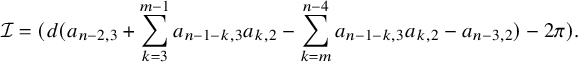 $$\begin{align*}\mathcal{I}=(d(a_{n-2,3}+\sum_{k=3}^{m-1}a_{n-1-k,3} a_{k,2}-\sum_{k=m}^{n-4}a_{n-1-k,3}a_{k,2}-a_{n-3,2})-2\pi). \end{align*}$$
It is easy to see that we have two irreducible components in the special fiber, where
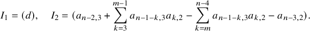 $$\begin{align*}I_1=(d),\quad I_2=(a_{n-2,3}+\sum_{k=3}^{m-1}a_{n-1-k,3} a_{k,2}-\sum_{k=m}^{n-4}a_{n-1-k,3}a_{k,2}-a_{n-3,2}). \end{align*}$$
Both irreducible components are isomorphic to $\mathbb {A}_k^{3(n-3)}$
, so they are smooth with the correct dimension. Their intersection is isomorphic to
$\mathbb {A}_k^{3(n-3)}$
, so they are smooth with the correct dimension. Their intersection is isomorphic to $\mathbb {A}_k^{3(n-3)-1}$
, which is also smooth. Since
$\mathbb {A}_k^{3(n-3)-1}$
, which is also smooth. Since $I_1, I_2$
are prime ideals, it is enough to prove that the special fiber
$I_1, I_2$
are prime ideals, it is enough to prove that the special fiber $V(\mathcal {I}_s)$
is reduced by showing
$V(\mathcal {I}_s)$
is reduced by showing $\mathcal {I}_s=I_1\cap I_2$
. By using similar arguments as in Proposition 5.2, we get that
$\mathcal {I}_s=I_1\cap I_2$
. By using similar arguments as in Proposition 5.2, we get that $V(\mathcal {I}_s)$
is reduced and
$V(\mathcal {I}_s)$
is reduced and $V(\mathcal {I})$
is regular.
$V(\mathcal {I})$
is regular.
In the second case, we can set $\Delta =\{1,\dots ,n-2\}/ \{m-1, m\}$
, and let
$\Delta =\{1,\dots ,n-2\}/ \{m-1, m\}$
, and let $i_2=m-1, i_3=m$
. Then
$i_2=m-1, i_3=m$
. Then $_2\mathcal {U}_{n-3,3}$
is isomorphic to
$_2\mathcal {U}_{n-3,3}$
is isomorphic to $V(\mathcal {J})=\mathrm {Spec \, } R'/\mathcal {J}$
, where
$V(\mathcal {J})=\mathrm {Spec \, } R'/\mathcal {J}$
, where
 $$\begin{align*}R'=O_F[x,d,z_{1,2},z_{1,3},(a_{i,1})_{i\in\Delta}, (a_{i,2})_{i\in\Delta}, (a_{i,3})_{i\in\Delta}], \end{align*}$$
and
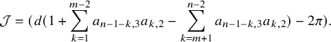 $$\begin{align*}\mathcal{J}=(d(1+\sum_{k=1}^{m-2}a_{n-1-k,3}a_{k,2}-\sum_{k=m+1}^{n-2}a_{n-1-k,3}a_{k,2})-2\pi). \end{align*}$$
Again, we have two irreducible components over the special fiber:
 $$\begin{align*}\mathcal{J}_1=(d),\quad \mathcal{J}_2=(1+\sum_{k=1}^{m-2}a_{n-1-k,3}a_{k,2}-\sum_{k=m+1}^{n-2}a_{n-1-k,3}a_{k,2}). \end{align*}$$
Both of them are smooth and of dimension $3(n-3)$
(Note that in this case, the second component
$3(n-3)$
(Note that in this case, the second component $V(\mathcal {J}_2)$
is not isomorphic to
$V(\mathcal {J}_2)$
is not isomorphic to $\mathbb {A}_k^{3(n-3)}$
). Their intersection is also smooth and of dimension
$\mathbb {A}_k^{3(n-3)}$
). Their intersection is also smooth and of dimension $3n-10$
. By using the same arguments as above, we can show that
$3n-10$
. By using the same arguments as above, we can show that $V(\mathcal {J}_s)$
is reduced and
$V(\mathcal {J}_s)$
is reduced and $V (\mathcal {J} )$
is regular. Thus,
$V (\mathcal {J} )$
is regular. Thus, $_2\mathcal {U}_{n-3,3}$
has semi-stable reduction over
$_2\mathcal {U}_{n-3,3}$
has semi-stable reduction over $O_F$
.
$O_F$
.
From Theorem 4.7 and Proposition 5.7, we have that $_2{\mathcal U}_{n-1,1}$
is smooth and
$_2{\mathcal U}_{n-1,1}$
is smooth and $_2{\mathcal U}_{n-3,3}$
has semi-stable reduction. Thus, both
$_2{\mathcal U}_{n-3,3}$
has semi-stable reduction. Thus, both $ _2{\mathcal U}_{n-1,1}$
and
$ _2{\mathcal U}_{n-1,1}$
and $_2{\mathcal U}_{n-3,3} $
are
$_2{\mathcal U}_{n-3,3} $
are $O_F$
-flat. As in §5.2, we deduce that these affine charts are open subschemes of the corresponding splitting model
$O_F$
-flat. As in §5.2, we deduce that these affine charts are open subschemes of the corresponding splitting model $\mathrm {M}^{\mathrm { spl}}$
. We will prove that
$\mathrm {M}^{\mathrm { spl}}$
. We will prove that $\mathrm {M}^{\mathrm {spl}}$
is smooth when
$\mathrm {M}^{\mathrm {spl}}$
is smooth when $(r,s)=(n-1,1)$
and
$(r,s)=(n-1,1)$
and $\mathrm {M}^{\mathrm {spl}}$
has semi-stable reduction when
$\mathrm {M}^{\mathrm {spl}}$
has semi-stable reduction when $(r,s)=(n-3,3)$
by showing that
$(r,s)=(n-3,3)$
by showing that ${\mathcal G}$
-translates of
${\mathcal G}$
-translates of $_2{\mathcal U}_{n-1,1}$
and
$_2{\mathcal U}_{n-1,1}$
and $_2{\mathcal U}_{n-3,3}$
cover
$_2{\mathcal U}_{n-3,3}$
cover $\mathrm {M}^{\mathrm {spl}}$
.
$\mathrm {M}^{\mathrm {spl}}$
.
Recall from §3 the ${\mathcal G}$
-equivariant morphism
${\mathcal G}$
-equivariant morphism $\tau : \mathrm {M}^{\mathrm {spl}}\rightarrow \mathrm {M}^{\mathrm {loc}} \otimes _{O}O_F$
which is given by
$\tau : \mathrm {M}^{\mathrm {spl}}\rightarrow \mathrm {M}^{\mathrm {loc}} \otimes _{O}O_F$
which is given by $(\mathcal {F}_0,\mathcal {F}_1)\mapsto \mathcal {F}_1$
and let
$(\mathcal {F}_0,\mathcal {F}_1)\mapsto \mathcal {F}_1$
and let $\tau _s: \mathrm {M}^{\mathrm {spl}}\otimes k\rightarrow \mathrm {M}^{\mathrm {loc}} \otimes k$
be the morphism over the special fiber. When s is odd, the unique closed
$\tau _s: \mathrm {M}^{\mathrm {spl}}\otimes k\rightarrow \mathrm {M}^{\mathrm {loc}} \otimes k$
be the morphism over the special fiber. When s is odd, the unique closed ${\mathcal G}$
-orbit of
${\mathcal G}$
-orbit of $\mathrm {M}^{\mathrm {loc}} \otimes k$
is the orbit of
$\mathrm {M}^{\mathrm {loc}} \otimes k$
is the orbit of $\Lambda '\otimes k$
(see §3). From the construction of the local model, it is enough to show that
$\Lambda '\otimes k$
(see §3). From the construction of the local model, it is enough to show that ${\mathcal G}_k$
-translates of
${\mathcal G}_k$
-translates of $_2\mathcal {U}_{n-1,1}\otimes k$
and
$_2\mathcal {U}_{n-1,1}\otimes k$
and $_2\mathcal {U}_{n-3,3}\otimes k$
cover
$_2\mathcal {U}_{n-3,3}\otimes k$
cover $\tau _s^{-1}(\Lambda '\otimes k)$
.
$\tau _s^{-1}(\Lambda '\otimes k)$
.
When $(r,s)=(n-1,1)$
, the inverse image
$(r,s)=(n-1,1)$
, the inverse image $\tau _s^{-1}(\Lambda '\otimes k)$
contains points
$\tau _s^{-1}(\Lambda '\otimes k)$
contains points $(\mathcal {F}_0,\Lambda '\otimes k)$
satisfying
$(\mathcal {F}_0,\Lambda '\otimes k)$
satisfying $t\Lambda '\subset \mathcal {F}_0$
. Observe that
$t\Lambda '\subset \mathcal {F}_0$
. Observe that $t\Lambda '=\text {span}_{k}\{-e_1\}$
and
$t\Lambda '=\text {span}_{k}\{-e_1\}$
and $\mathcal {F}_0$
has rank
$\mathcal {F}_0$
has rank $1$
. Thus,
$1$
. Thus, $\tau _s^{-1}(\Lambda '\otimes k)=(\text {span}_{k}\{-e_1\}, \Lambda '\otimes k)$
is just a unique point (Note that it is different from the case when s is even, see §5.2, where we have
$\tau _s^{-1}(\Lambda '\otimes k)=(\text {span}_{k}\{-e_1\}, \Lambda '\otimes k)$
is just a unique point (Note that it is different from the case when s is even, see §5.2, where we have $t\Lambda _m=0$
). From §4.2, we see that
$t\Lambda _m=0$
). From §4.2, we see that $_2\mathcal {U}_{n-1,1}\otimes k$
contains that point and so
$_2\mathcal {U}_{n-1,1}\otimes k$
contains that point and so ${\mathcal G}_k$
-translates of
${\mathcal G}_k$
-translates of $_2\mathcal {U}_{n-1,1}\otimes k$
cover
$_2\mathcal {U}_{n-1,1}\otimes k$
cover $\tau _s^{-1}(\Lambda '\otimes k)$
. Hence,
$\tau _s^{-1}(\Lambda '\otimes k)$
. Hence, ${\mathcal G}$
-translates of
${\mathcal G}$
-translates of $_2\mathcal {U}_{n-1,1}$
cover
$_2\mathcal {U}_{n-1,1}$
cover $\mathrm {M}^{\mathrm {spl}}$
.
$\mathrm {M}^{\mathrm {spl}}$
.
When s is odd and $\geq 3$
, we have
$\geq 3$
, we have
 $$\begin{align*}\tau_s^{-1}(\Lambda'\otimes k)=\{(\mathcal{F}_0,\Lambda')\mid \text{span}_{k}\{-e_1\}\subset \mathcal{F}_0\subset \Lambda'\otimes k,\quad t\mathcal{F}_0=(0)\}. \end{align*}$$
Set $\mathcal {F}_0=\text {span}_k\{e_1, v_2, \dots , v_s\}$
. Then
$\mathcal {F}_0=\text {span}_k\{e_1, v_2, \dots , v_s\}$
. Then $t\mathcal {F}_0=0$
and
$t\mathcal {F}_0=0$
and $\mathcal {F}_0\subset \Lambda '\otimes k$
imply that
$\mathcal {F}_0\subset \Lambda '\otimes k$
imply that $v_2, \dots , v_s$
are a linear combination of
$v_2, \dots , v_s$
are a linear combination of $\{-e_2,\dots , -e_m, \pi e_{m+1},\dots , \pi e_{n-1}\}$
. Thus, we consider the morphism
$\{-e_2,\dots , -e_m, \pi e_{m+1},\dots , \pi e_{n-1}\}$
. Thus, we consider the morphism
 $$\begin{align*}\pi: \tau_s^{-1}(\Lambda'\otimes k)\rightarrow \mathrm{Gr}(s-1,n-2)\otimes k \end{align*}$$
given by $(\mathcal {F}_0,\Lambda ')\mapsto \text {span}_k\{v_2, \cdots , v_s\}$
. Here,
$(\mathcal {F}_0,\Lambda ')\mapsto \text {span}_k\{v_2, \cdots , v_s\}$
. Here, $\mathrm {Gr}(s-1,n-2)\otimes k$
is the Grassmannian of
$\mathrm {Gr}(s-1,n-2)\otimes k$
is the Grassmannian of $(s-1)$
-dimensional subspaces of
$(s-1)$
-dimensional subspaces of
 $$\begin{align*}\Lambda'/\{-\pi^{-1}e_1, -e_1\}=\text{span}_k\{-e_2,\dots, -e_m, \pi e_{m+1},\dots, \pi e_{n-1}\}. \end{align*}$$
We also have a section
 $$\begin{align*}\phi: \mathrm{Gr}(s-1,n-2)\otimes k\rightarrow \mathrm{M}^{\mathrm{spl}}\otimes k, \end{align*}$$
given by $W\rightarrow (\text {span}_k(e_1, W),\Lambda ')$
. Similar to §5.2, it is easy to see that the image of the section
$W\rightarrow (\text {span}_k(e_1, W),\Lambda ')$
. Similar to §5.2, it is easy to see that the image of the section $\phi $
is
$\phi $
is $\tau _s^{-1}(\Lambda '\otimes k)$
. Hence,
$\tau _s^{-1}(\Lambda '\otimes k)$
. Hence, $\tau _s^{-1}(\Lambda '\otimes k)$
is isomorphic to
$\tau _s^{-1}(\Lambda '\otimes k)$
is isomorphic to $\mathrm {Gr}(s-1,n-2)\otimes k$
. As in §5.2, we can equip
$\mathrm {Gr}(s-1,n-2)\otimes k$
. As in §5.2, we can equip $\tau _s^{-1}(\Lambda '\otimes k)$
with a nondegenerate alternating form; that is,
$\tau _s^{-1}(\Lambda '\otimes k)$
with a nondegenerate alternating form; that is, $\langle tv,tw\rangle ':=(tv,w)=v^tJ_{n-2}w$
for
$\langle tv,tw\rangle ':=(tv,w)=v^tJ_{n-2}w$
for $tv, tw\in \tau _s^{-1}(\Lambda '\otimes k)$
. Denote by
$tv, tw\in \tau _s^{-1}(\Lambda '\otimes k)$
. Denote by $\mathcal {Q}(s-1,n-2)$
the closed subscheme of
$\mathcal {Q}(s-1,n-2)$
the closed subscheme of $\mathrm {Gr}(s-1,n-2)\otimes k$
which parametrizes all isotropic
$\mathrm {Gr}(s-1,n-2)\otimes k$
which parametrizes all isotropic $(s-1)$
-subspaces with respect to
$(s-1)$
-subspaces with respect to $\langle \ , \ \rangle '$
.
$\langle \ , \ \rangle '$
.
The following observations concern the special fiber of $_2{\mathcal U}_{r,s}$
when s is odd. We keep the same notation as in §4.2.
$_2{\mathcal U}_{r,s}$
when s is odd. We keep the same notation as in §4.2.
Remark 5.8. (1) Set $\mathbf {a}_i$
the i-th column of the matrix
$\mathbf {a}_i$
the i-th column of the matrix $M_2$
;
$M_2$
; $\mathbf {a}_i$
can be expressed as the element
$\mathbf {a}_i$
can be expressed as the element $tv\in \tau _s^{-1}(\Lambda '\otimes k)$
, where
$tv\in \tau _s^{-1}(\Lambda '\otimes k)$
, where $tv=[ 0~0~a_{1,i}~\cdots ~a_{n-2,i}\mid ~0~\cdots ~ 0]^t$
. Thus,
$tv=[ 0~0~a_{1,i}~\cdots ~a_{n-2,i}\mid ~0~\cdots ~ 0]^t$
. Thus,
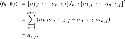 $$ \begin{align*} \langle \mathbf{a}_i,\mathbf{a}_j\rangle' &=[a_{1,i}~\cdots ~a_{n-2,i}]J_{n-2}[a_{1,j}~\cdots ~a_{n-2,j}]^t \\ &=\sum_{k=1}^{m-1}(a_{k,i}a_{n-1-k.j}-a_{n-1-k.i}a_{k,j})\\ &= q_{i,j}. \end{align*} $$
(2) For the special fiber $\mathrm {M}^{\mathrm {spl}}\otimes k$
, consider
$\mathrm {M}^{\mathrm {spl}}\otimes k$
, consider $(_2\mathcal {U}_{r,s}\otimes k) \cap \tau _s^{-1}(\Lambda '\otimes k)$
. We get
$(_2\mathcal {U}_{r,s}\otimes k) \cap \tau _s^{-1}(\Lambda '\otimes k)$
. We get $C=0$
since
$C=0$
since $A=0$
. The first column of C is
$A=0$
. The first column of C is $\mathbf {a}_1+z_{1,2}\mathbf {a}_2+\cdots +z_{1,s}\mathbf {a}_s$
. By setting
$\mathbf {a}_1+z_{1,2}\mathbf {a}_2+\cdots +z_{1,s}\mathbf {a}_s$
. By setting $i=i_2, \dots , i_s$
, this gives us
$i=i_2, \dots , i_s$
, this gives us $z_{1,2}=\cdots =z_{1,s}=0$
and so
$z_{1,2}=\cdots =z_{1,s}=0$
and so $\mathbf {a}_1=\mathbf {0}$
. Thus,
$\mathbf {a}_1=\mathbf {0}$
. Thus,
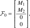 $$\begin{align*}\mathcal{F}_0=\left[\begin{array}{c} M_1\\ M_2\\ \hline 0\\ 0 \end{array}\right], \end{align*}$$
where
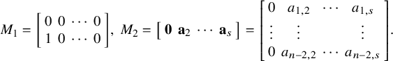 $$\begin{align*}M_1=\left[\begin{array}{cccc} 0& 0&\cdots & 0\\ 1& 0&\cdots &0 \end{array}\right],~ M_2=\left[\begin{array}{cccc} \mathbf{0} & \mathbf{a}_2 &\cdots &\mathbf{a}_s \end{array}\right]= \left[\begin{array}{cccc} 0 & a_{1,2}&\cdots & a_{1,s}\\ \vdots &\vdots &&\vdots\\ 0& a_{n-2,2}& \cdots & a_{n-2,s}\\ \end{array}\right]. \end{align*}$$
By definition, $Q=[q_{i,j}]=0$
is equivalent to
$Q=[q_{i,j}]=0$
is equivalent to $\langle \mathbf {a}_i,\mathbf {a}_j \rangle '=0$
for
$\langle \mathbf {a}_i,\mathbf {a}_j \rangle '=0$
for $2\leq i, j\leq s$
. Therefore,
$2\leq i, j\leq s$
. Therefore, $\pi (\mathcal {F}_0)$
is totally isotropic under
$\pi (\mathcal {F}_0)$
is totally isotropic under $\langle ~,~ \rangle '$
if and only if
$\langle ~,~ \rangle '$
if and only if $Q=0$
(which actually occurs). Thus,
$Q=0$
(which actually occurs). Thus,
 $$\begin{align*}\phi(\mathcal{Q}(s-1,n-2))\subset (_2\mathcal{U}_{r,s}\otimes k)\cap \tau_s^{-1}(\Lambda'\otimes k). \end{align*}$$
Theorem 5.9. When $(r,s)=(n-3,3)$
,
$(r,s)=(n-3,3)$
, ${\mathcal G}$
-translates of
${\mathcal G}$
-translates of $_2\mathcal {U}_{n-3,3}$
cover
$_2\mathcal {U}_{n-3,3}$
cover $\mathrm {M}^{\mathrm {spl}}$
.
$\mathrm {M}^{\mathrm {spl}}$
.
Proof. It is enough to prove that ${\mathcal G}$
-translates of
${\mathcal G}$
-translates of $_2\mathcal {U}_{n-3,3}$
cover
$_2\mathcal {U}_{n-3,3}$
cover $\tau ^{-1}(\Lambda ')$
. We use similar arguments as in the proof of Theorem 5.4. Since
$\tau ^{-1}(\Lambda ')$
. We use similar arguments as in the proof of Theorem 5.4. Since $\mathcal {G}_k$
acts on
$\mathcal {G}_k$
acts on $\tau _s^{-1}(\Lambda '\otimes k)\simeq \mathrm {Gr}(2,n-2)\otimes k$
, this action factors through the symplectic group
$\tau _s^{-1}(\Lambda '\otimes k)\simeq \mathrm {Gr}(2,n-2)\otimes k$
, this action factors through the symplectic group $Sp(n-2)_k$
of the symplectic form
$Sp(n-2)_k$
of the symplectic form $\langle \,,\,\rangle '$
on
$\langle \,,\,\rangle '$
on $ \Lambda '/ \{-\pi ^{-1}e_1, -e_1\} $
, and gives the surjective map
$ \Lambda '/ \{-\pi ^{-1}e_1, -e_1\} $
, and gives the surjective map $ \mathcal {G}_k \rightarrow Sp(n-2)_k$
, where
$ \mathcal {G}_k \rightarrow Sp(n-2)_k$
, where
 $$\begin{align*}Sp(n-2)_k=\{g\in SL(n-2)_k\mid g^tJ_{n-2}g=J_{n-2}\}. \end{align*}$$
By [Reference Barbasch and Evens3, §3], the $Sp(n-2)_k$
-action on
$Sp(n-2)_k$
-action on $\mathrm {Gr}(2,n-2)\otimes k$
has two orbits:
$\mathrm {Gr}(2,n-2)\otimes k$
has two orbits: $Q(0)$
and
$Q(0)$
and $Q(2)$
, where
$Q(2)$
, where
 $$\begin{align*}Q(i)=\{\mathcal{F}_0\in \mathrm{Gr}(2,n-2)\mid \dim(rad(\mathcal{F}_0))=i\}, \end{align*}$$
for $i=0, 2$
. Similar to the proof of Theorem 5.4, we have
$i=0, 2$
. Similar to the proof of Theorem 5.4, we have $Q(2)\subset \overline {Q(0)}$
. Thus,
$Q(2)\subset \overline {Q(0)}$
. Thus, $Q(2)$
is the unique closed orbit. Observe that
$Q(2)$
is the unique closed orbit. Observe that $Q(2)$
contains all totally isotropic subspaces
$Q(2)$
contains all totally isotropic subspaces $\pi (\mathcal {F}_0)$
, and so
$\pi (\mathcal {F}_0)$
, and so $Q(2)= \mathcal {Q}(2,n-2)$
.
$Q(2)= \mathcal {Q}(2,n-2)$
.
From Remark 5.8 (2), we have that $_2{\mathcal U}_{n-3,3}\otimes k$
contains points
$_2{\mathcal U}_{n-3,3}\otimes k$
contains points $(\mathcal {F}_0,\Lambda '\otimes k)$
with
$(\mathcal {F}_0,\Lambda '\otimes k)$
with $\pi (\mathcal {F}_0) \in \mathcal {Q}(2,n-2) $
. By identifying
$\pi (\mathcal {F}_0) \in \mathcal {Q}(2,n-2) $
. By identifying $\tau _s^{-1}(\Lambda '\otimes k)$
with
$\tau _s^{-1}(\Lambda '\otimes k)$
with $\mathrm {Gr}(2,n-2)\otimes k$
, we get that
$\mathrm {Gr}(2,n-2)\otimes k$
, we get that $_2{\mathcal U}_{n-3,3}$
contains points from all the orbits. Therefore, from all the above, we deduce that the
$_2{\mathcal U}_{n-3,3}$
contains points from all the orbits. Therefore, from all the above, we deduce that the $\mathcal {G}$
-translates of
$\mathcal {G}$
-translates of $_2{\mathcal U}_{n-3,3}$
cover
$_2{\mathcal U}_{n-3,3}$
cover $\tau ^{-1}(\Lambda ')$
.
$\tau ^{-1}(\Lambda ')$
.
From Propositions 4.7 and 5.7 and Theorem 5.9, we have the following:
Corollary 5.10.
-
a) When
$(r,s)=(n-1,1)$
,
$\mathrm {M}^{\mathrm {spl}}$
is a smooth scheme. -
b) When
$(r,s)=(n-3,3)$
,
$\mathrm {M}^{\mathrm {spl}}$
has semi-stable reduction over
$O_F$
. In particular,
$\mathrm {M}^{\mathrm {spl}}$
is regular and has special fiber a reduced divisor with two smooth irreducible components intersecting transversely.


Remark 5.11. For s odd and $\geq 5$
, note that we have
$\geq 5$
, note that we have
 $$\begin{align*}\pi: \tau_{s}^{-1}(\Lambda'\otimes k)\stackrel{\sim}{\rightarrow} \mathrm{Gr}(s-1,n-2)\otimes k, \end{align*}$$
and
 $$\begin{align*}\mathcal{Q}(s-1,n-2)\subset (_2{\mathcal U}_{r,s}\otimes k)\cap \tau^{-1}_s(\Lambda\otimes k). \end{align*}$$
If we can show that the affine chart $_2{\mathcal U}_{r,s}$
is flat, then we have
$_2{\mathcal U}_{r,s}$
is flat, then we have $_2{\mathcal U}_{r,s}\subset \mathrm {M}^{\mathrm {spl}}$
. By using a similar argument as the proof of Theorem 5.9, we could prove that
$_2{\mathcal U}_{r,s}\subset \mathrm {M}^{\mathrm {spl}}$
. By using a similar argument as the proof of Theorem 5.9, we could prove that ${\mathcal G}$
-translates of
${\mathcal G}$
-translates of $_2{\mathcal U}_{r,s}$
cover
$_2{\mathcal U}_{r,s}$
cover $\mathrm {M}^{\mathrm {spl}}$
.
$\mathrm {M}^{\mathrm {spl}}$
.
Remark 5.12. When $ (r,s) = (n-1,1)$
, the local model
$ (r,s) = (n-1,1)$
, the local model $ \mathrm {M}^{\mathrm {loc}} \subset \mathrm {M}^{\wedge }$
is smooth (see [Reference Pappas and Rapoport18, §5.3]). Consider the morphism
$ \mathrm {M}^{\mathrm {loc}} \subset \mathrm {M}^{\wedge }$
is smooth (see [Reference Pappas and Rapoport18, §5.3]). Consider the morphism $\tau : \mathrm {M}^{\mathrm {spl}} \longrightarrow \mathrm {M}^{\mathrm {loc}} \otimes _{O} O_F$
. The generic fiber of all of these is the same (see §3). In particular, from all the above discussion in this section, we can see that
$\tau : \mathrm {M}^{\mathrm {spl}} \longrightarrow \mathrm {M}^{\mathrm {loc}} \otimes _{O} O_F$
. The generic fiber of all of these is the same (see §3). In particular, from all the above discussion in this section, we can see that $ \mathrm {M}^{\mathrm {spl}} \cong \mathrm {M}^{\mathrm {loc}} \otimes _{O} O_{F}$
.
$ \mathrm {M}^{\mathrm {spl}} \cong \mathrm {M}^{\mathrm {loc}} \otimes _{O} O_{F}$
.
6 Application to Shimura varieties
In this section, we give the most immediate application of Corollaries 5.5 and 5.10 to unitary Shimura varieties. Indeed, by using work of Rapoport and Zink [Reference Rapoport and Zink24], we first construct p-adic integral models for the signatures $ (n-s,s)$
with
$ (n-s,s)$
with $ s\leq 3$
where the level subgroup at p is the special maximal parahoric subgroup
$ s\leq 3$
where the level subgroup at p is the special maximal parahoric subgroup $P_{\{m\}}$
defined in §2.2. These models have simple and explicit moduli descriptions and are étale locally around each point isomorphic to naive local models. Then by using the above corollaries and producing a linear modification, we obtain smooth integral models of the corresponding Shimura varieties when
$P_{\{m\}}$
defined in §2.2. These models have simple and explicit moduli descriptions and are étale locally around each point isomorphic to naive local models. Then by using the above corollaries and producing a linear modification, we obtain smooth integral models of the corresponding Shimura varieties when $s=1$
and semi-stable models when
$s=1$
and semi-stable models when $s=2$
or
$s=2$
or $s=3$
(i.e., they are regular and the irreducible components of the special fiber are smooth divisors crossing normally). (See Theorem 6.1.)
$s=3$
(i.e., they are regular and the irreducible components of the special fiber are smooth divisors crossing normally). (See Theorem 6.1.)
We start with an imaginary quadratic field K and we fix an embedding $\varepsilon : K\rightarrow \mathbb {C}$
. Let W be a n-dimensional K-vector space, equipped with a nondegenerate hermitian form
$\varepsilon : K\rightarrow \mathbb {C}$
. Let W be a n-dimensional K-vector space, equipped with a nondegenerate hermitian form $\phi $
. Consider the group
$\phi $
. Consider the group $G = \mathrm {GU}_n$
of unitary similitudes for
$G = \mathrm {GU}_n$
of unitary similitudes for $(W,\phi )$
of dimension
$(W,\phi )$
of dimension $n\geq 3$
over K. Assume that
$n\geq 3$
over K. Assume that $n=2m$
is even. We fix a conjugacy class of homomorphisms
$n=2m$
is even. We fix a conjugacy class of homomorphisms $h: \mathrm {Res}_{\mathbb {C}/\mathbb {R}}\mathbb {G}_{m,\mathbb {C}}\rightarrow \mathrm {GU}_n$
corresponding to a Shimura datum
$h: \mathrm {Res}_{\mathbb {C}/\mathbb {R}}\mathbb {G}_{m,\mathbb {C}}\rightarrow \mathrm {GU}_n$
corresponding to a Shimura datum $(G,X) = (\mathrm {GU}_n,X_h)$
of signature
$(G,X) = (\mathrm {GU}_n,X_h)$
of signature $(r,s)$
. The pair
$(r,s)$
. The pair $(G,X)$
gives rise to a Shimura variety
$(G,X)$
gives rise to a Shimura variety $\mathrm {Sh}(G,X)$
over the reflex field E. (See [Reference Pappas and Rapoport18, §1.1] and [Reference Pappas15, §3] for more details on the description of the unitary Shimura varieties.) Let p be an odd prime number which ramifies in K. Set
$\mathrm {Sh}(G,X)$
over the reflex field E. (See [Reference Pappas and Rapoport18, §1.1] and [Reference Pappas15, §3] for more details on the description of the unitary Shimura varieties.) Let p be an odd prime number which ramifies in K. Set $K_1=K\otimes _{\mathbb {Q}} \mathbb {Q}_p$
with a uniformizer
$K_1=K\otimes _{\mathbb {Q}} \mathbb {Q}_p$
with a uniformizer $\pi $
, and
$\pi $
, and $V=W\otimes _{\mathbb {Q}} \mathbb {Q}_p$
. We assume that the hermitian form
$V=W\otimes _{\mathbb {Q}} \mathbb {Q}_p$
. We assume that the hermitian form $\phi $
is split on V (i.e., there is a basis
$\phi $
is split on V (i.e., there is a basis $e_1, \dots , e_n$
such that
$e_1, \dots , e_n$
such that $\phi (e_i, e_{n+1-j})=\delta _{ij}$
for
$\phi (e_i, e_{n+1-j})=\delta _{ij}$
for $1\leq i, j\leq n$
). We denote by
$1\leq i, j\leq n$
). We denote by
 $$\begin{align*}\Lambda_i = \text{span}_{O_{K_1}} \{\pi^{-1}e_1, \dots, \pi^{-1}e_i, e_{i+1}, \dots, e_n\} \end{align*}$$
the standard lattices in V. We can complete this into a self dual lattice chain by setting $\Lambda _{i+kn}:=\pi ^{-k}\Lambda _i$
(see §2.1). Denote by
$\Lambda _{i+kn}:=\pi ^{-k}\Lambda _i$
(see §2.1). Denote by $P_{\{m\}}$
the stabilizer of
$P_{\{m\}}$
the stabilizer of $\Lambda _m$
in
$\Lambda _m$
in $G(\mathbb {Q}_p)$
. We let
$G(\mathbb {Q}_p)$
. We let $\mathcal {L}$
be the self-dual multichain consisting of lattices
$\mathcal {L}$
be the self-dual multichain consisting of lattices $\{\Lambda _j\}_{j\in n\mathbb {Z} \pm m}$
. Here,
$\{\Lambda _j\}_{j\in n\mathbb {Z} \pm m}$
. Here, $\mathcal {G} = \underline {\mathrm {Aut}}(\mathcal {L})$
is the (smooth) group scheme over
$\mathcal {G} = \underline {\mathrm {Aut}}(\mathcal {L})$
is the (smooth) group scheme over $\mathbb {Z}_p$
with
$\mathbb {Z}_p$
with $P_{\{m\}} = \mathcal {G}(\mathbb {Z}_p)$
the subgroup of
$P_{\{m\}} = \mathcal {G}(\mathbb {Z}_p)$
the subgroup of $G(\mathbb {Q}_p)$
fixing the lattice chain
$G(\mathbb {Q}_p)$
fixing the lattice chain $\mathcal {L}$
.
$\mathcal {L}$
.
Choose also a sufficiently small compact open subgroup $K^p$
of the prime-to-p finite adelic points
$K^p$
of the prime-to-p finite adelic points $G({\mathbb A}_{f}^p)$
of G and set
$G({\mathbb A}_{f}^p)$
of G and set $\mathbf {K}=K^pP_{\{m\}}$
. The Shimura variety
$\mathbf {K}=K^pP_{\{m\}}$
. The Shimura variety $\mathrm { Sh}_{\mathbf {K}}(G, X)$
with complex points
$\mathrm { Sh}_{\mathbf {K}}(G, X)$
with complex points
 $$\begin{align*}\mathrm{Sh}_{\mathbf{K}}(G, X)(\mathbb{C})=G(\mathbb{Q})\backslash X\times G({\mathbb A}_{f})/\mathbf{K} \end{align*}$$
is of PEL type and has a canonical model over the reflex field E. We set $\mathcal {O} = O_{E_v}$
, where v the unique prime ideal of E above
$\mathcal {O} = O_{E_v}$
, where v the unique prime ideal of E above $(p)$
.
$(p)$
.
We consider the moduli functor $\mathcal {A}^{\mathrm {naive}}_{\mathbf {K}}$
over
$\mathcal {A}^{\mathrm {naive}}_{\mathbf {K}}$
over $\mathrm {Spec \, } \mathcal {O} $
given in [Reference Rapoport and Zink24, Definition 6.9]:
$\mathrm {Spec \, } \mathcal {O} $
given in [Reference Rapoport and Zink24, Definition 6.9]:
A point of $\mathcal {A}^{\mathrm {naive}}_{\mathbf {K}}$
with values in the
$\mathcal {A}^{\mathrm {naive}}_{\mathbf {K}}$
with values in the $\mathcal {O} $
-scheme S is the isomorphism class of the following set of data
$\mathcal {O} $
-scheme S is the isomorphism class of the following set of data $(A,\iota ,\bar {\lambda }, \bar {\eta })$
:
$(A,\iota ,\bar {\lambda }, \bar {\eta })$
:
-
(1) An object
$(A,\iota )$
, where A is an abelian scheme with relative dimension n over S (terminology of [Reference Rapoport and Zink24]), compatibly endowed with an action of
${\mathcal O}$
:
$$\begin{align*}\iota: {\mathcal O} \rightarrow \text{End} \,A \otimes \mathbb{Z}_p.\end{align*}$$
-
(2) A
$\mathbb {Q}$
-homogeneous principal polarization
$\bar {\lambda }$
of the
$\mathcal {L}$
-set A. -
(3) A
$K^p$
-level structure which respects the bilinear forms on both sides up to a constant in
$$\begin{align*}\bar{\eta} : H_1 (A, {\mathbb A}_{f}^p) \simeq W \otimes {\mathbb A}_{f}^p \, \text{ mod} \, K^p \end{align*}$$
$({\mathbb A}_{f}^p)^{\times }$
(see loc. cit. for details).
The set A should satisfy the determinant condition (i) of loc. cit.


For the definitions of the terms employed here, we refer to loc.cit., 6.3–6.8 and [Reference Pappas15, §3]. The functor $\mathcal {A}^{\mathrm {naive}}_{\mathbf {K}}$
is representable by a quasi-projective scheme over
$\mathcal {A}^{\mathrm {naive}}_{\mathbf {K}}$
is representable by a quasi-projective scheme over $\mathcal {O}$
. Since the Hasse principle is satisfied for the unitary group, we can see as in loc. cit. that there is a natural isomorphism
$\mathcal {O}$
. Since the Hasse principle is satisfied for the unitary group, we can see as in loc. cit. that there is a natural isomorphism
 $$\begin{align*}\mathcal{A}^{\mathrm{naive}}_{\mathbf{K}} \otimes_{{\mathcal O}} E_v = \mathrm{Sh}_{\mathbf{K}}(G, X)\otimes_{E} E_v. \end{align*}$$
As is explained in [Reference Rapoport and Zink24] and [Reference Pappas15], the naive local model $\mathrm {M}^{\mathrm {naive}}$
is connected to the moduli scheme
$\mathrm {M}^{\mathrm {naive}}$
is connected to the moduli scheme $\mathcal {A}^{\mathrm {naive}}_{\mathbf {K}}$
via the local model diagram
$\mathcal {A}^{\mathrm {naive}}_{\mathbf {K}}$
via the local model diagram
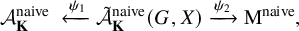 $$\begin{align*}\mathcal{A}^{\mathrm{naive}}_{\mathbf{K}} \ \xleftarrow{\psi_1} \tilde{\mathcal{A}}^{\mathrm{naive}}_{\mathbf{K}} (G,X) \xrightarrow{\psi_2} \mathrm{M}^{\mathrm{naive}}, \end{align*}$$
where the morphism $\psi _1$
is a
$\psi _1$
is a $\mathcal {G}$
-torsor and
$\mathcal {G}$
-torsor and $\psi _2$
is a smooth and
$\psi _2$
is a smooth and $\mathcal {G}$
-equivariant morphism. Therefore, there is a relatively representable smooth morphism
$\mathcal {G}$
-equivariant morphism. Therefore, there is a relatively representable smooth morphism
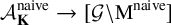 $$\begin{align*}\mathcal{A}^{\mathrm{naive}}_{\mathbf{K}} \to [\mathcal{G} \backslash \mathrm{M}^{\mathrm{naive}}] \end{align*}$$
where the target is the quotient algebraic stack.
Next, denote by $ \mathcal {A}^{\mathrm {flat}}_{\mathbf {K}} $
the flat closure of
$ \mathcal {A}^{\mathrm {flat}}_{\mathbf {K}} $
the flat closure of $\mathrm {Sh}_{\mathbf {K}}(G, X)\otimes _{E} E_v$
in
$\mathrm {Sh}_{\mathbf {K}}(G, X)\otimes _{E} E_v$
in $ \mathcal {A}^{\mathrm {naive}}_{\mathbf {K}}$
. Recall from §3 that the flat closure of
$ \mathcal {A}^{\mathrm {naive}}_{\mathbf {K}}$
. Recall from §3 that the flat closure of $ \mathrm {M}^{\mathrm {naive}} \otimes _{\mathcal {O}} E_v$
in
$ \mathrm {M}^{\mathrm {naive}} \otimes _{\mathcal {O}} E_v$
in $\mathrm {M}^{\mathrm {naive}}$
is by definition the local model
$\mathrm {M}^{\mathrm {naive}}$
is by definition the local model $\mathrm {M}^{\mathrm {loc}} $
. By the above, we can see, as in [Reference Pappas and Rapoport18], that there is a relatively representable smooth morphism of relative dimension
$\mathrm {M}^{\mathrm {loc}} $
. By the above, we can see, as in [Reference Pappas and Rapoport18], that there is a relatively representable smooth morphism of relative dimension $\mathrm {dim} (G)$
,
$\mathrm {dim} (G)$
,
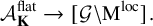 $$\begin{align*}\mathcal{A}^{\mathrm{flat}}_{\mathbf{K}} \to [\mathcal{G} \backslash \mathrm{M}^{\mathrm{loc}}].\end{align*}$$
This of course implies that $\mathcal {A}^{\mathrm {flat}}_{\mathbf {K}}$
is étale locally isomorphic to the local model
$\mathcal {A}^{\mathrm {flat}}_{\mathbf {K}}$
is étale locally isomorphic to the local model $\mathrm {M}^{\mathrm {loc}}$
.
$\mathrm {M}^{\mathrm {loc}}$
.
One can now consider a variation of the moduli of abelian schemes $\mathcal {A}_{\mathbf {K}}$
where we add in the moduli problem an additional subspace in the Hodge filtration
$\mathcal {A}_{\mathbf {K}}$
where we add in the moduli problem an additional subspace in the Hodge filtration $ \mathrm {Fil}^0 (A) \subset H_{dR}^1(A)$
of the universal abelian variety A (see [Reference Haines7, §6.3] for more details) with certain conditions to imitate the definition of the naive splitting model
$ \mathrm {Fil}^0 (A) \subset H_{dR}^1(A)$
of the universal abelian variety A (see [Reference Haines7, §6.3] for more details) with certain conditions to imitate the definition of the naive splitting model $\mathcal {M}$
. (See §3 for the definition of naive splitting models.) More precisely,
$\mathcal {M}$
. (See §3 for the definition of naive splitting models.) More precisely, $\mathcal {A}_{\mathbf {K}}$
associates to an
$\mathcal {A}_{\mathbf {K}}$
associates to an $O_{K_1}$
-scheme S the set of isomorphism classes of objects
$O_{K_1}$
-scheme S the set of isomorphism classes of objects $(A,\iota ,\bar {\lambda }, \bar {\eta },\mathscr {F}_0) $
. Here,
$(A,\iota ,\bar {\lambda }, \bar {\eta },\mathscr {F}_0) $
. Here, $(A,\iota ,\bar {\lambda }, \bar {\eta })$
is an object of
$(A,\iota ,\bar {\lambda }, \bar {\eta })$
is an object of $\mathcal {A}^{\mathrm {naive}}_{\mathbf {K}}(S).$
Set
$\mathcal {A}^{\mathrm {naive}}_{\mathbf {K}}(S).$
Set $\mathscr {F}_1 := \mathrm {Fil}^0 (A) $
. The final ingredient
$\mathscr {F}_1 := \mathrm {Fil}^0 (A) $
. The final ingredient $\mathscr {F}_0$
of an object of
$\mathscr {F}_0$
of an object of $\mathcal {A}_{\mathbf {K}}$
is the subspace
$\mathcal {A}_{\mathbf {K}}$
is the subspace $ \mathscr {F}_0 \subset \mathscr {F}_1 \subset H_{dR}^1(A) $
of rank s which satisfies the following conditions:
$ \mathscr {F}_0 \subset \mathscr {F}_1 \subset H_{dR}^1(A) $
of rank s which satisfies the following conditions:
 $$\begin{align*}(\iota(\pi)+\pi ) \mathscr{F}_1 \subset \mathscr{F}_0, \quad (\iota(\pi)-\pi )\mathscr{F}_0 = (0). \end{align*}$$
There is a forgetful projective morphism
 $$\begin{align*}\tau_1 : \mathcal{A}_{\mathbf{K}} \longrightarrow \mathcal{A}^{\mathrm{naive}}_{\mathbf{K}}\otimes_{\mathcal{O}} O_{K_1} \end{align*}$$
defined by $(A,\iota ,\bar {\lambda }, \bar {\eta },\mathscr {F}_0) \mapsto (A,\iota ,\bar {\lambda }, \bar {\eta }) $
. Moreover,
$(A,\iota ,\bar {\lambda }, \bar {\eta },\mathscr {F}_0) \mapsto (A,\iota ,\bar {\lambda }, \bar {\eta }) $
. Moreover, $\mathcal {A}_{\mathbf {K}}$
has the same étale local structure as
$\mathcal {A}_{\mathbf {K}}$
has the same étale local structure as $\mathcal {M}$
; it is a ‘linear modification’ of
$\mathcal {M}$
; it is a ‘linear modification’ of $\mathcal {A}^{\mathrm {naive}}_{\mathbf {K}}\otimes _{\mathcal {O}} O_{K_1}$
in the sense of [Reference Pappas15, §2] (see also [Reference Pappas and Rapoport17, §15]). As we showed in Proposition 5.1, the scheme
$\mathcal {A}^{\mathrm {naive}}_{\mathbf {K}}\otimes _{\mathcal {O}} O_{K_1}$
in the sense of [Reference Pappas15, §2] (see also [Reference Pappas and Rapoport17, §15]). As we showed in Proposition 5.1, the scheme $\mathcal {M}$
is never flat, and by the above, the same is true for
$\mathcal {M}$
is never flat, and by the above, the same is true for $\mathcal {A}_{\mathbf {K}}$
.
$\mathcal {A}_{\mathbf {K}}$
.
Theorem 6.1. Assume that $ (r,s) = (n-1,1)$
or
$ (r,s) = (n-1,1)$
or $(n-2,2)$
or
$(n-2,2)$
or $(n-3,3)$
. For every
$(n-3,3)$
. For every $K^p$
as above, there is a scheme
$K^p$
as above, there is a scheme $\mathcal {A}^{\mathrm {spl}}_{\mathbf {K}}$
, flat over
$\mathcal {A}^{\mathrm {spl}}_{\mathbf {K}}$
, flat over $\mathrm {Spec \, } (O_{K_1})$
, with
$\mathrm {Spec \, } (O_{K_1})$
, with
 $$\begin{align*}\mathcal{A}^{\mathrm{spl}}_{\mathbf{K}}\otimes_{O_{K_1}} K_1=\mathrm{Sh}_{\mathbf{K}}(G, X)\otimes_{E} K_1, \end{align*}$$
and which supports a local model diagram

such that
-
a)
$\pi ^{\mathrm {reg}}_{\mathbf {K}}$
is a
$\mathcal {G}$
-torsor for the parahoric group scheme
${\mathcal G}$
that corresponds to
$P_{\{m\}}$
. -
b)
$q^{\mathrm {reg}}_{\mathbf {K}}$
is smooth and
${\mathcal G}$
-equivariant. -
c) When
$(r,s) = (n-1,1)$
,
$\mathcal {A}^{\mathrm {spl}}_{\mathbf {K}}$
is a smooth scheme. -
c’) When
$(r,s) = (n-2,2)$
or
$(r,s) =(n-3,3)$
,
$\mathcal {A}^{\mathrm {spl}}_{\mathbf {K}}$
is regular and has special fiber which is a reduced divisor with normal crossings.


Proof. From the above, we have the local model diagram
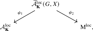
where the morphism $\psi _1$
is a
$\psi _1$
is a $\mathcal {G}$
-torsor and
$\mathcal {G}$
-torsor and $\psi _2$
is a smooth and
$\psi _2$
is a smooth and $\mathcal {G}$
-equivariant morphism. Set
$\mathcal {G}$
-equivariant morphism. Set
 $$\begin{align*}\widetilde{\mathcal{A}}^{\mathrm{spl}}_{\mathbf{K}}(G, X)=\widetilde{\mathcal{A}}^{\mathrm{loc}}_{\mathbf{K}}(G, X)\times_{\mathrm{M}^{\mathrm{loc}}}\mathrm{M}^{\mathrm{spl}}, \end{align*}$$
which carries a diagonal $\mathcal {G}$
-action. Since
$\mathcal {G}$
-action. Since $\tau : \mathrm {M}^{\mathrm {spl}} \rightarrow \mathrm {M}^{\mathrm {loc}}\otimes _{O} O_F$
is projective (see §5), we can see ([Reference Pappas15, §2]) that the quotient
$\tau : \mathrm {M}^{\mathrm {spl}} \rightarrow \mathrm {M}^{\mathrm {loc}}\otimes _{O} O_F$
is projective (see §5), we can see ([Reference Pappas15, §2]) that the quotient
 $$\begin{align*}\pi^{\mathrm{reg}}_K: \widetilde{\mathcal{A}}^{\mathrm{spl}}_{\mathbf{K}} \longrightarrow \mathcal{A}^{\mathrm{spl}}_{\mathbf{K}}:={\mathcal G}\backslash \widetilde{\mathcal{A} }^{\mathrm{spl}}_K(G, X) \end{align*}$$
is represented by a scheme and gives a ${\mathcal G}$
-torsor. (Recall that the morphism
${\mathcal G}$
-torsor. (Recall that the morphism $\tau $
induces an isomorphism on the generic fibers.) This is an example of a linear modification; see [Reference Pappas15, §2]. The projection gives a smooth
$\tau $
induces an isomorphism on the generic fibers.) This is an example of a linear modification; see [Reference Pappas15, §2]. The projection gives a smooth ${\mathcal G}$
-morphism
${\mathcal G}$
-morphism
 $$\begin{align*}q^{\mathrm{reg}}_{\mathbf{K}}: \widetilde{\mathcal{A}}^{\mathrm{spl}}_{\mathbf{K}} \longrightarrow \mathrm{M}^{\mathrm{spl}} \end{align*}$$
which completes the local model diagram. Property (c) (resp. (c’)) follows from Theorem 5.10 (resp. Corollaries 5.5 and 5.10) and properties (a) and (b) which imply that $ \mathcal {A}^{\mathrm {spl}}_{\mathbf {K}}$
and
$ \mathcal {A}^{\mathrm {spl}}_{\mathbf {K}}$
and $ \mathrm {M}^{\mathrm {spl}}$
are locally isomorphic for the étale topology.
$ \mathrm {M}^{\mathrm {spl}}$
are locally isomorphic for the étale topology.
Remarks 6.2. Similar results can be obtained for corresponding Rapoport-Zink formal schemes. (See [Reference He, Pappas and Rapoport12, §4] for an example of this parallel treatment.)
7 Moduli description of
$\mathrm {M}^{\mathrm {spl}}$

In this section, we show that by adding the ‘spin condition’ in the naive splitting model $\mathcal {M}$
, we get the splitting model
$\mathcal {M}$
, we get the splitting model $\mathrm {M}^{\mathrm {spl}}$
for signature
$\mathrm {M}^{\mathrm {spl}}$
for signature $s\leq 3$
.
$s\leq 3$
.
We use the notation of §2, §3, and we set $ W= \wedge ^{n}_F (V\otimes _{F_0}F).$
Recall that the symmetric form
$ W= \wedge ^{n}_F (V\otimes _{F_0}F).$
Recall that the symmetric form $( \, , \, )$
splits over V, and thus, there is a canonical decomposition
$( \, , \, )$
splits over V, and thus, there is a canonical decomposition
 $$\begin{align*}W = W_1 \oplus W_{-1} \end{align*}$$
of $W $
as an
$W $
as an $\mathrm {SO}_{2n} \left ((\, ,\,)\right )(F)$
-representation (see [Reference Rapoport, Smithling and Zhang23, §7], [Reference Smithling27, §2]). For a standard lattice
$\mathrm {SO}_{2n} \left ((\, ,\,)\right )(F)$
-representation (see [Reference Rapoport, Smithling and Zhang23, §7], [Reference Smithling27, §2]). For a standard lattice $\Lambda _i$
in V (see §2), we set
$\Lambda _i$
in V (see §2), we set $W(\Lambda _i)=\wedge ^n(\Lambda _i\otimes _{O_{F_0}}O_F )$
and
$W(\Lambda _i)=\wedge ^n(\Lambda _i\otimes _{O_{F_0}}O_F )$
and $W(\Lambda _i)_{\pm 1 } = W_{\pm 1} \cap W(\Lambda ).$
For an
$W(\Lambda _i)_{\pm 1 } = W_{\pm 1} \cap W(\Lambda ).$
For an $O_F$
-scheme S and
$O_F$
-scheme S and $\epsilon \in \{\pm 1\}$
, we set
$\epsilon \in \{\pm 1\}$
, we set
 $$\begin{align*}L_{i,\epsilon}(S)=\text{im}[ W(\Lambda_i)_{\epsilon}\otimes_{O_F} \mathcal{O}_S \longrightarrow W(\Lambda)\otimes_{O_F} \mathcal{O}_S ]. \end{align*}$$
We now formulate the spin condition:
(5) (Spin condition) the line bundle $\wedge ^n \mathcal {F}_1 \subset W(\Lambda _m)\otimes _{O_F} \mathcal {O}_S$
is contained in
$\wedge ^n \mathcal {F}_1 \subset W(\Lambda _m)\otimes _{O_F} \mathcal {O}_S$
is contained in $ L_{m,(-1)^s}(S)$
.
$ L_{m,(-1)^s}(S)$
.
The spin splitting model $\mathcal {M}^{\mathrm {spin}}$
is the closed subscheme of
$\mathcal {M}^{\mathrm {spin}}$
is the closed subscheme of $\mathcal {M}$
defined by imposing the spin condition. We have the following inclusions of closed subschemes
$\mathcal {M}$
defined by imposing the spin condition. We have the following inclusions of closed subschemes $\mathrm { M}^{\mathrm {spl}}\subset \mathcal {M}^{\mathrm {spin}}\subset \mathcal {M}$
which are all equalities between generic fibers (see [Reference Pappas and Rapoport18, §7] and [Reference Rapoport, Smithling and Zhang23, §9]). The restriction of
$\mathrm { M}^{\mathrm {spl}}\subset \mathcal {M}^{\mathrm {spin}}\subset \mathcal {M}$
which are all equalities between generic fibers (see [Reference Pappas and Rapoport18, §7] and [Reference Rapoport, Smithling and Zhang23, §9]). The restriction of $\tau $
on
$\tau $
on $\mathcal {M}^{\mathrm {spin}}$
gives us
$\mathcal {M}^{\mathrm {spin}}$
gives us
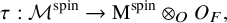 $$\begin{align*}\tau : \mathcal{M}^{\mathrm{spin}} \rightarrow \mathrm{M}^{\mathrm{spin}}\otimes_{O} O_F, \end{align*}$$
where $\mathrm {M}^{\mathrm {spin}}$
is the spin local model defined in [Reference Pappas and Rapoport18]. In particular,
$\mathrm {M}^{\mathrm {spin}}$
is the spin local model defined in [Reference Pappas and Rapoport18]. In particular, $\mathrm {M}^{\mathrm {spin}}$
is the closed subscheme of
$\mathrm {M}^{\mathrm {spin}}$
is the closed subscheme of $\mathrm {M}^{\wedge }$
that classifies points given by
$\mathrm {M}^{\wedge }$
that classifies points given by $\mathcal {F}_1$
which satisfy the spin condition. We want to mention that Smithling [Reference Smithling26, Theorem 1.3] proved that
$\mathcal {F}_1$
which satisfy the spin condition. We want to mention that Smithling [Reference Smithling26, Theorem 1.3] proved that $\mathrm {M}^{\mathrm {spin}}$
is topologically flat. Also, from [Reference Rapoport, Smithling and Zhang23, Remark 9.9], we get that the spin condition can be characterized as the following condition:
$\mathrm {M}^{\mathrm {spin}}$
is topologically flat. Also, from [Reference Rapoport, Smithling and Zhang23, Remark 9.9], we get that the spin condition can be characterized as the following condition:
(5’) The rank of $ (t+ \pi )$
on
$ (t+ \pi )$
on $\mathcal {F}_1$
has the same parity as s.Footnote
1
$\mathcal {F}_1$
has the same parity as s.Footnote
1
Remark 7.1. Recall from the proof of Proposition 5.1 that the point $(\mathcal {F}_0, t\Lambda _m)$
when s is odd and the point
$(\mathcal {F}_0, t\Lambda _m)$
when s is odd and the point $(\mathcal {F}_0, \Lambda ')$
when s is even does not lift to the generic fiber. However, we can easily see that these points do not satisfy the condition (5’) and so they are not in
$(\mathcal {F}_0, \Lambda ')$
when s is even does not lift to the generic fiber. However, we can easily see that these points do not satisfy the condition (5’) and so they are not in $\mathcal {M}^{\mathrm {spin}}$
.
$\mathcal {M}^{\mathrm {spin}}$
.
Proposition 7.2.
-
a) When s is even,
$_1{\mathcal U}_{r,s}\subset {\mathcal {M}}^{\mathrm {spin}}$
. -
b) When s is odd,
$_2{\mathcal U}_{r,s}\subset {\mathcal {M}}^{\mathrm {spin}}$
.


Proof. It is enough to consider the rank $((t+\pi )\mathcal {F}_1)$
over the special fiber (
$((t+\pi )\mathcal {F}_1)$
over the special fiber ( $\pi = 0$
) for the following two cases.
$\pi = 0$
) for the following two cases.
Case 1: Consider the affine chart $_1{\mathcal U}_{r,s}$
around
$_1{\mathcal U}_{r,s}$
around $(\mathcal {F}_0, \Lambda _m)$
. Recall from §4.1 that
$(\mathcal {F}_0, \Lambda _m)$
. Recall from §4.1 that
 $$\begin{align*}\mathcal{F}_1 = \left[\begin{array}{@{}c@{}} A\\ \hline I_n \end{array} \right], \quad \mathcal{F}_0 = \left[\begin{array}{@{}c@{}} X_1\\ \hline X_2 \end{array} \right]. \end{align*}$$
By $(t + \pi ) \mathcal {F}_1 \subset \mathcal {F}_0$
, we get
$(t + \pi ) \mathcal {F}_1 \subset \mathcal {F}_0$
, we get
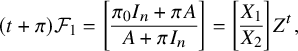 $$\begin{align*}(t+\pi)\mathcal{F}_1= \left[\begin{array}{@{}c@{}} \pi_0I_n + \pi A \\ \hline A + \pi I_n \end{array} \right] = \left[\begin{array}{@{}c@{}} X_1 \\ \hline X_2 \end{array} \right]Z^t, \end{align*}$$
where Z is of size $n\times s$
. Since rank
$n\times s$
. Since rank $(\mathcal {F}_0)=s$
, the rank of
$(\mathcal {F}_0)=s$
, the rank of $(t + \pi ) \mathcal {F}_1$
amounts to rank
$(t + \pi ) \mathcal {F}_1$
amounts to rank $(Z^t)$
. Note that
$(Z^t)$
. Note that $Z^t = D^t\cdot \widetilde {Y}^t$
, where D is of size
$Z^t = D^t\cdot \widetilde {Y}^t$
, where D is of size $s\times s$
and rank
$s\times s$
and rank $(\widetilde {Y})=s$
. Thus, rank
$(\widetilde {Y})=s$
. Thus, rank $(Z^t)=$
rank
$(Z^t)=$
rank $(D^t)$
. Since D is a skew-symmetric matrix, the rank of D is always an even number. Therefore the rank of
$(D^t)$
. Since D is a skew-symmetric matrix, the rank of D is always an even number. Therefore the rank of $(t+\pi )\mathcal {F}_1$
, where
$(t+\pi )\mathcal {F}_1$
, where $(\mathcal {F}_0, \mathcal {F}_1)\in \, _{1}{\mathcal U}_{r,s}$
, is always even.
$(\mathcal {F}_0, \mathcal {F}_1)\in \, _{1}{\mathcal U}_{r,s}$
, is always even.
Case 2: Consider the affine chart $_2{\mathcal U}_{r,s}$
around
$_2{\mathcal U}_{r,s}$
around $(\mathcal {F}_0, \Lambda ')$
. In this case, from §4.2, we have
$(\mathcal {F}_0, \Lambda ')$
. In this case, from §4.2, we have
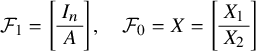 $$\begin{align*}\mathcal{F}_1=\left[\begin{array}{c} I_n\\ \hline A \end{array} \right],\quad \mathcal{F}_0=X=\left[\begin{array}{c} X_1\\ \hline X_2 \end{array} \right] \end{align*}$$
and
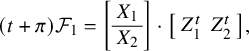 $$\begin{align*}(t+\pi)\mathcal{F}_1= \left[\begin{array}{c} X_1\\ \hline X_2 \end{array} \right]\cdot \left[\begin{array}{cc} Z_1^t & Z_2^t \end{array} \right], \end{align*}$$
where $Z_1$
is of size
$Z_1$
is of size $2\times s$
and
$2\times s$
and $Z_2$
is of size
$Z_2$
is of size $(n-2)\times s$
. Thus, the rank of
$(n-2)\times s$
. Thus, the rank of $(t + \pi ) \mathcal {F}_1$
amounts to rank
$(t + \pi ) \mathcal {F}_1$
amounts to rank $([Z_1^t\ Z_2^t])$
. Over the special fiber, we have
$([Z_1^t\ Z_2^t])$
. Over the special fiber, we have
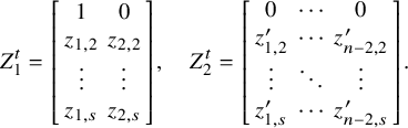 $$\begin{align*}Z_1^t=\left[\begin{array}{cc} 1& 0 \\ z_{1,2} & z_{2,2}\\ \vdots &\vdots\\ z_{1,s} & z_{2,s} \end{array} \right], \quad Z_2^t=\left[\begin{array}{ccc} 0&\cdots & 0 \\ z_{1,2}'&\cdots & z_{n-2,2}'\\ \vdots & \ddots & \vdots \\ z_{1,s}'&\cdots & z_{n-2,s}' \end{array} \right]. \end{align*}$$
We treat $Z_1^t, Z_2^t$
separately. By (4.2.1),
$Z_1^t, Z_2^t$
separately. By (4.2.1), $Z_2^t$
can be expressed as
$Z_2^t$
can be expressed as
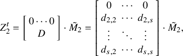 $$\begin{align*}Z_2^t=\left[\begin{array}{c}0\cdots 0\\ D\end{array}\right]\cdot \tilde{M}_2= \left[\begin{array}{ccc} 0&\cdots &0\\ d_{2,2}&\cdots & d_{2,s}\\ \vdots &\ddots &\vdots\\ d_{s,2}&\cdots & d_{s,s} \end{array}\right]\cdot \tilde{M}_2, \end{align*}$$
where D is a skew-symmetric matrix, and $\tilde {M}_2$
contains an
$\tilde {M}_2$
contains an $I_{s-1}$
-minor. Thus,
$I_{s-1}$
-minor. Thus, $Z_2^t$
is generated by the columns of
$Z_2^t$
is generated by the columns of $\left [\begin {array}{c}0\cdots 0\\ D\end {array}\right ]$
. For
$\left [\begin {array}{c}0\cdots 0\\ D\end {array}\right ]$
. For $Z_1^t$
, we claim that the second column is generated by
$Z_1^t$
, we claim that the second column is generated by $\left [\begin {array}{c}0\cdots 0\\ D\end {array}\right ]$
. From (4.2.2), we have
$\left [\begin {array}{c}0\cdots 0\\ D\end {array}\right ]$
. From (4.2.2), we have
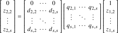 $$\begin{align*}\left[\begin{array}{c} 0\\ z_{2,2}\\ \vdots\\ z_{2,s} \end{array}\right]=\left[\begin{array}{ccc} 0&\cdots&0\\ d_{2,2}&\cdots & d_{2,s}\\ \vdots &\ddots & \vdots\\ d_{s,2}&\cdots & d_{s,s} \end{array}\right] \left[\begin{array}{ccc} q_{2,1}&\cdots & q_{2,s}\\ \vdots &\ddots & \vdots\\ q_{s,1}&\cdots & q_{s,s} \end{array}\right] \left[\begin{array}{c} 1\\ z_{1,2}\\ \vdots\\ z_{1,s} \end{array}\right] \end{align*}$$
in the special fiber. Recall that $D\cdot Q=0$
, where
$D\cdot Q=0$
, where
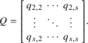 $$\begin{align*}Q=\left[\begin{array}{ccc} q_{2,2}&\cdots & q_{2,s}\\ \vdots &\ddots &\vdots\\ q_{s,2}&\cdots & q_{s,s} \end{array}\right]. \end{align*}$$
Then
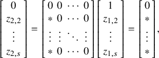 $$\begin{align*}\left[\begin{array}{c} 0\\ z_{2,2}\\ \vdots\\ z_{2,s} \end{array}\right]=\left[\begin{array}{cccc} 0&0&\cdots &0\\ *&0 &\cdots & 0\\ \vdots&\vdots &\ddots & \vdots\\ *& 0&\cdots & 0 \end{array}\right] \left[\begin{array}{c} 1\\ z_{1,2}\\ \vdots\\ z_{1,s} \end{array}\right]= \left[\begin{array}{c} 0\\ *\\ \vdots\\ * \end{array}\right], \end{align*}$$
which can be expressed as
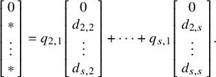 $$\begin{align*}\left[\begin{array}{c} 0\\ *\\ \vdots\\ * \end{array}\right]=q_{2,1}\left[\begin{array}{c} 0\\ d_{2,2}\\ \vdots\\ d_{s,2} \end{array}\right]+\cdots +q_{s,1} \left[\begin{array}{c} 0\\ d_{2,s}\\ \vdots\\ d_{s,s} \end{array}\right]. \end{align*}$$
Therefore, the second column is generated by $\left [\begin {array}{c}0\cdots 0\\ D\end {array}\right ]$
. From all the above, we deduce that the rank of
$\left [\begin {array}{c}0\cdots 0\\ D\end {array}\right ]$
. From all the above, we deduce that the rank of $[Z_1^t\ Z_2^t]$
amounts to the rank of
$[Z_1^t\ Z_2^t]$
amounts to the rank of
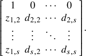 $$\begin{align*}\left[\begin{array}{cccc} 1& 0 &\cdots &0\\ z_{1,2} & d_{2,2}& \cdots & d_{2,s}\\ \vdots &\vdots& \ddots&\vdots\\ z_{1,s} & d_{s,2}&\cdots & d_{s,s} \end{array} \right]. \end{align*}$$
Since rank(D) is even, and the first column is linear independent to the rest of the columns, the rank of $(t+\pi )\mathcal {F}_1$
, where
$(t+\pi )\mathcal {F}_1$
, where $(\mathcal {F}_0, \mathcal {F}_1)\in _{2}{\mathcal U}_{r,s}$
, is always odd.
$(\mathcal {F}_0, \mathcal {F}_1)\in _{2}{\mathcal U}_{r,s}$
, is always odd.
Therefore, $_1{\mathcal U}_{r,s}\subset {\mathcal {M}}^{\mathrm {spin}}$
if and only if s is even and
$_1{\mathcal U}_{r,s}\subset {\mathcal {M}}^{\mathrm {spin}}$
if and only if s is even and $_2{\mathcal U}_{r,s}\subset {\mathcal {M}}^{\mathrm {spin}}$
if and only if s is odd.
$_2{\mathcal U}_{r,s}\subset {\mathcal {M}}^{\mathrm {spin}}$
if and only if s is odd.
In particular, when $s=2$
, we have
$s=2$
, we have $_{1}{\mathcal U}_{n-2,2}\subset \mathcal {M}^{\mathrm {spin}}$
, and when
$_{1}{\mathcal U}_{n-2,2}\subset \mathcal {M}^{\mathrm {spin}}$
, and when $s=3$
, we have
$s=3$
, we have $_{2}{\mathcal U}_{n-3,3}\subset \mathcal {M}^{\mathrm {spin}}$
. Moreover, since
$_{2}{\mathcal U}_{n-3,3}\subset \mathcal {M}^{\mathrm {spin}}$
. Moreover, since $\mathrm {M}^{\mathrm {spin}}$
is topologically flat, or in other words, the underlying topological spaces of
$\mathrm {M}^{\mathrm {spin}}$
is topologically flat, or in other words, the underlying topological spaces of $\mathrm {M}^{\mathrm {spin}}$
and
$\mathrm {M}^{\mathrm {spin}}$
and $\mathrm {M}^{\mathrm {loc}}$
coincide, we can repeat the
$\mathrm {M}^{\mathrm {loc}}$
coincide, we can repeat the $\mathcal {G}$
-translates argument as in Theorems 5.4 and 5.9 and obtain the following.
$\mathcal {G}$
-translates argument as in Theorems 5.4 and 5.9 and obtain the following.
Proposition 7.3.
-
a) When
$(r,s)=(n-2,2)$
,
${\mathcal G}$
-translates of
$_1\mathcal {U}_{n-2,2}$
cover
$\mathcal {M}^{\mathrm {spin}}$
. -
b) When
$(r,s)=(n-3,3)$
,
${\mathcal G}$
-translates of
$_2\mathcal {U}_{n-3,3}$
cover
$\mathcal {M}^{\mathrm {spin}}$
.


From Theorems 5.4, 5.9 and Proposition 7.3, we deduce the following.
Theorem 7.4. For the signatures $(n-s,s)$
with
$(n-s,s)$
with $s\leq 3$
, we have
$s\leq 3$
, we have $\mathcal {M}^{\mathrm {spin}}=\mathrm {M}^{\mathrm {spl}}$
.
$\mathcal {M}^{\mathrm {spin}}=\mathrm {M}^{\mathrm {spl}}$
.
Therefore, we obtain a moduli-theoretic description of $\mathrm {M}^{\mathrm {spl}}$
and by Theorem 6.1 for the corresponding integral model
$\mathrm {M}^{\mathrm {spl}}$
and by Theorem 6.1 for the corresponding integral model $\mathcal {A}^{\mathrm {spl}}_{\mathbf {K}}$
. In particular, the closed subscheme
$\mathcal {A}^{\mathrm {spl}}_{\mathbf {K}}$
. In particular, the closed subscheme $\mathcal {A}^{\mathrm {spl}}_{\mathbf {K}} \subset \mathcal {A}_{\mathbf {K}}$
(see §6 for the explicit definition of
$\mathcal {A}^{\mathrm {spl}}_{\mathbf {K}} \subset \mathcal {A}_{\mathbf {K}}$
(see §6 for the explicit definition of $\mathcal {A}_{\mathbf {K}}$
) is obtained by imposing the following additional condition on the moduli problem of
$\mathcal {A}_{\mathbf {K}}$
) is obtained by imposing the following additional condition on the moduli problem of $\mathcal {A}_{\mathbf {K}}$
:
$\mathcal {A}_{\mathbf {K}}$
:
Spin condition. The rank of $(\iota (\pi ) + \pi )$
on
$(\iota (\pi ) + \pi )$
on $\mathrm {Fil}^0(A)$
has the same parity as s.
$\mathrm {Fil}^0(A)$
has the same parity as s.
Remark 7.5. Recall the ${\mathcal G}$
-equivariant morphism
${\mathcal G}$
-equivariant morphism $\tau : \mathrm {M}^{\mathrm {spl}}\rightarrow \mathrm {M}^{\mathrm {loc}}\otimes _O O_F$
, which is given by
$\tau : \mathrm {M}^{\mathrm {spl}}\rightarrow \mathrm {M}^{\mathrm {loc}}\otimes _O O_F$
, which is given by $(\mathcal {F}_0, \mathcal {F}_1)\mapsto \mathcal {F}_1$
. By the above remark, we have
$(\mathcal {F}_0, \mathcal {F}_1)\mapsto \mathcal {F}_1$
. By the above remark, we have $\mathcal {M}^{\mathrm {spin}}=\mathrm {M}^{\mathrm {spl}}$
for the signatures
$\mathcal {M}^{\mathrm {spin}}=\mathrm {M}^{\mathrm {spl}}$
for the signatures $(n-s,s)$
with
$(n-s,s)$
with $s\leq 3$
. Define
$s\leq 3$
. Define $\tau _s: \mathrm {M}^{\mathrm {spl}}\otimes k\rightarrow \mathrm {M}^{\mathrm {loc}}\otimes k$
over the special fiber. For a point
$\tau _s: \mathrm {M}^{\mathrm {spl}}\otimes k\rightarrow \mathrm {M}^{\mathrm {loc}}\otimes k$
over the special fiber. For a point $ (\mathcal {F}_0, \mathcal {F}_1) \in \mathrm {M}^{\mathrm {spl}}\otimes k$
, we have
$ (\mathcal {F}_0, \mathcal {F}_1) \in \mathrm {M}^{\mathrm {spl}}\otimes k$
, we have $(0) \subset t \mathcal {F}_1\subset \mathcal {F}_0$
and
$(0) \subset t \mathcal {F}_1\subset \mathcal {F}_0$
and $t\mathcal {F}_0 = (0)$
which gives
$t\mathcal {F}_0 = (0)$
which gives $(0)\subset \mathcal {F}_0 \subset t\Lambda _m \otimes k$
. Also, we have
$(0)\subset \mathcal {F}_0 \subset t\Lambda _m \otimes k$
. Also, we have
 $$\begin{align*}\begin{array}{ll} \mathcal{F}_1 \subset \mathcal{F}_0^{\bot}, & t\Lambda_m\otimes k \subset \mathcal{F}_0^{\bot},\\ \mathcal{F}_1 \subset t^{-1}(\mathcal{F}_0), & t\Lambda_m\otimes k \subset t^{-1}(\mathcal{F}_0). \end{array} \end{align*}$$
The spaces $t^{-1}(\mathcal {F}_0) , \,\mathcal {F}_0^{\bot }$
have rank
$t^{-1}(\mathcal {F}_0) , \,\mathcal {F}_0^{\bot }$
have rank $n + s$
,
$n + s$
, $2n-s$
, respectively, and we indicate with
$2n-s$
, respectively, and we indicate with $ \bot $
the orthogonal complement with respect to
$ \bot $
the orthogonal complement with respect to $(\,,\,)$
. From above, we obtain that
$(\,,\,)$
. From above, we obtain that
 $$ \begin{align} \mathcal{F}_1\subset \mathcal{F}_1+t\Lambda_m\otimes k \subset \mathcal{F}_0^{\bot}\cap t^{-1}(\mathcal{F}_0)\subset t^{-1}(\mathcal{F}_0). \end{align} $$
A) When the signature $(r,s)=(n-2,2)$
, we have a morphism
$(r,s)=(n-2,2)$
, we have a morphism $\pi : \mathrm {M}^{\mathrm {spl}}\otimes k\rightarrow \mathrm {Gr}(2,n)\otimes k$
given by
$\pi : \mathrm {M}^{\mathrm {spl}}\otimes k\rightarrow \mathrm {Gr}(2,n)\otimes k$
given by $(\mathcal {F}_0, \mathcal {F}_1)\mapsto \mathcal {F}_0$
. Let
$(\mathcal {F}_0, \mathcal {F}_1)\mapsto \mathcal {F}_0$
. Let $M_1=\tau _s^{-1}(t\Lambda _m\otimes k)$
, and
$M_1=\tau _s^{-1}(t\Lambda _m\otimes k)$
, and $M_2=\pi ^{-1}(\mathcal {Q}(2,n))$
. Recall that
$M_2=\pi ^{-1}(\mathcal {Q}(2,n))$
. Recall that $M_1$
is isomorphic to the Grassmannian
$M_1$
is isomorphic to the Grassmannian $\mathrm {Gr}(2,n)\otimes k$
of dimension
$\mathrm {Gr}(2,n)\otimes k$
of dimension $2n-4$
. The spin condition translates to: rank(
$2n-4$
. The spin condition translates to: rank( $t\mathcal {F}_1)=$
even. Since
$t\mathcal {F}_1)=$
even. Since $0\subset t\mathcal {F}_1\subset \mathcal {F}_0$
, we get rank
$0\subset t\mathcal {F}_1\subset \mathcal {F}_0$
, we get rank $(t\mathcal {F}_1)=0$
or
$(t\mathcal {F}_1)=0$
or $2$
, (i.e.,
$2$
, (i.e., $t\mathcal {F}_1=0$
or
$t\mathcal {F}_1=0$
or $t\mathcal {F}_1=\mathcal {F}_0$
).
$t\mathcal {F}_1=\mathcal {F}_0$
).
Furthermore, from $t\mathcal {F}_1=0$
, we get
$t\mathcal {F}_1=0$
, we get $\mathcal {F}_1\subset t\Lambda _m\otimes k$
which implies
$\mathcal {F}_1\subset t\Lambda _m\otimes k$
which implies $\mathcal {F}_1=t\Lambda _m\otimes k$
, so
$\mathcal {F}_1=t\Lambda _m\otimes k$
, so $(\mathcal {F}_0, \mathcal {F}_1)\in M_1$
. However, if
$(\mathcal {F}_0, \mathcal {F}_1)\in M_1$
. However, if $t\mathcal {F}_1=\mathcal {F}_0$
, we have rank
$t\mathcal {F}_1=\mathcal {F}_0$
, we have rank $(t(\mathcal {F}_1+t\Lambda _m\otimes k))=$
rank
$(t(\mathcal {F}_1+t\Lambda _m\otimes k))=$
rank $(t\mathcal {F}_1)=2$
. Thus, rank
$(t\mathcal {F}_1)=2$
. Thus, rank $(\mathcal {F}_1+t\Lambda _m\otimes k)\geq n+2$
. By rank
$(\mathcal {F}_1+t\Lambda _m\otimes k)\geq n+2$
. By rank $(t^{-1}(\mathcal {F}_0))=n+2$
and (7.0.1), we get
$(t^{-1}(\mathcal {F}_0))=n+2$
and (7.0.1), we get $\mathcal {F}_1+t\Lambda _m\otimes k = \mathcal {F}_0^{\bot }\cap t^{-1}(\mathcal {F}_0)= t^{-1}(\mathcal {F}_0)$
, which implies
$\mathcal {F}_1+t\Lambda _m\otimes k = \mathcal {F}_0^{\bot }\cap t^{-1}(\mathcal {F}_0)= t^{-1}(\mathcal {F}_0)$
, which implies $ t^{-1}(\mathcal {F}_0) \subset \mathcal {F}_0^{\bot }$
. As in [Reference Zachos28, §2.1], observe that
$ t^{-1}(\mathcal {F}_0) \subset \mathcal {F}_0^{\bot }$
. As in [Reference Zachos28, §2.1], observe that $ \mathcal {F}_0 \in \mathcal {Q}(2,n)$
(i.e.,
$ \mathcal {F}_0 \in \mathcal {Q}(2,n)$
(i.e., $ \langle \mathcal {F}_0,\mathcal {F}_0 \rangle ' = 0$
) is equivalent to
$ \langle \mathcal {F}_0,\mathcal {F}_0 \rangle ' = 0$
) is equivalent to $\text {rank} \, (t^{-1}(\mathcal {F}_0) \cap \mathcal {F}^{\bot }_0) = n+2 $
(i.e.,
$\text {rank} \, (t^{-1}(\mathcal {F}_0) \cap \mathcal {F}^{\bot }_0) = n+2 $
(i.e., $ t^{-1}(\mathcal {F}_0) \subset \mathcal {F}_0^{\bot })$
. So
$ t^{-1}(\mathcal {F}_0) \subset \mathcal {F}_0^{\bot })$
. So $(\mathcal {F}_0, \mathcal {F}_1)\in M_2$
.
$(\mathcal {F}_0, \mathcal {F}_1)\in M_2$
.
Therefore, $\mathrm {M}^{\mathrm {spl}}\otimes k = M_1 \cup M_2$
. Moreover, from the above, we can easily see that
$\mathrm {M}^{\mathrm {spl}}\otimes k = M_1 \cup M_2$
. Moreover, from the above, we can easily see that $\tau ': M_2\setminus M_1\simeq \mathrm {M}^{\mathrm {loc}} \setminus \{t\Lambda _m\otimes k\}$
, so that
$\tau ': M_2\setminus M_1\simeq \mathrm {M}^{\mathrm {loc}} \setminus \{t\Lambda _m\otimes k\}$
, so that $M_2$
maps birationally to the special fiber of
$M_2$
maps birationally to the special fiber of $\mathrm {M}^{\mathrm {loc}}$
.
$\mathrm {M}^{\mathrm {loc}}$
.
Lastly, the fiber $\pi ^{-1}(\{\mathcal {F}_0\}) $
with
$\pi ^{-1}(\{\mathcal {F}_0\}) $
with $\mathcal {F}_0 \in \mathcal {Q}(2,n) $
contains all
$\mathcal {F}_0 \in \mathcal {Q}(2,n) $
contains all $(\mathcal {F}_0, \mathcal {F}_1) $
with
$(\mathcal {F}_0, \mathcal {F}_1) $
with $\mathcal {F}_1$
satisfying
$\mathcal {F}_1$
satisfying $\mathcal {F}_0 \subset (t^{-1}(\mathcal {F}_0))^{\bot } \subset \mathcal {F}_1 \subset t^{-1}(\mathcal {F}_0).$
These
$\mathcal {F}_0 \subset (t^{-1}(\mathcal {F}_0))^{\bot } \subset \mathcal {F}_1 \subset t^{-1}(\mathcal {F}_0).$
These $ \{\mathcal {F}_1\}$
correspond to isotropic, with respect to
$ \{\mathcal {F}_1\}$
correspond to isotropic, with respect to $( \,,\,)$
, subspaces in the four-dimensional space
$( \,,\,)$
, subspaces in the four-dimensional space $t^{-1}(\mathcal {F}_0)/ (t^{-1}(\mathcal {F}_0))^{\bot }$
, and they are parameterized by the orthogonal Grassmannian
$t^{-1}(\mathcal {F}_0)/ (t^{-1}(\mathcal {F}_0))^{\bot }$
, and they are parameterized by the orthogonal Grassmannian $ \mathrm {OGr}(2,4)$
. Therefore,
$ \mathrm {OGr}(2,4)$
. Therefore, $M_2$
is a
$M_2$
is a $\mathrm {OGr}(2,4)$
-bundle over
$\mathrm {OGr}(2,4)$
-bundle over $ \mathcal {Q}(2,n)$
with dimension
$ \mathcal {Q}(2,n)$
with dimension $2n-4$
, and
$2n-4$
, and $M_1, M_2$
intersect transversally over the smooth scheme
$M_1, M_2$
intersect transversally over the smooth scheme $\mathcal {Q}(2,n)$
of rank
$\mathcal {Q}(2,n)$
of rank $2n-5$
.
$2n-5$
.
B) When the signature $(r,s)=(n-3,3)$
, the unique closed
$(r,s)=(n-3,3)$
, the unique closed $\mathcal {G}$
-orbit in
$\mathcal {G}$
-orbit in $\mathrm {M}^{\mathrm {loc}}\otimes k$
is not the point
$\mathrm {M}^{\mathrm {loc}}\otimes k$
is not the point $t\Lambda _m\otimes k$
but the orbit of
$t\Lambda _m\otimes k$
but the orbit of $\Lambda '\otimes k$
which we denote by
$\Lambda '\otimes k$
which we denote by $O_{wt}$
. Let
$O_{wt}$
. Let
 $$\begin{align*}M_1=\tau_s^{-1}(O_{wt})=\{(\mathcal{F}_0, \mathcal{F}_1)\in \mathrm{M}^{\mathrm{spl}}\otimes k\mid \mathcal{F}_1=g\cdot \Lambda' ~\text{for some}~ g\in{\mathcal G}\} \end{align*}$$
and
 $$\begin{align*}M_2=\{(\mathcal{F}_0, \mathcal{F}_1)\in \mathrm{M}^{\mathrm{spl}}\otimes k\mid \mathcal{F}_0 ~\text{is totally isotropic under}~ \langle \ ,\ \rangle'\}. \end{align*}$$
The spin condition translates to rank $(t\mathcal {F}_1)=$
odd. By
$(t\mathcal {F}_1)=$
odd. By $0\subset t\mathcal {F}_1\subset \mathcal {F}_0$
, we get rank
$0\subset t\mathcal {F}_1\subset \mathcal {F}_0$
, we get rank $(t\mathcal {F}_1)=1$
or
$(t\mathcal {F}_1)=1$
or $3$
.
$3$
.
If rank $(t\mathcal {F}_1)=3$
, we have
$(t\mathcal {F}_1)=3$
, we have $t\mathcal {F}_1=\mathcal {F}_0$
which implies rank
$t\mathcal {F}_1=\mathcal {F}_0$
which implies rank $(\mathcal {F}_1+t\Lambda _m\otimes k)\geq n+3$
. By (7.0.1), we get
$(\mathcal {F}_1+t\Lambda _m\otimes k)\geq n+3$
. By (7.0.1), we get $\mathcal {F}_0^{\bot }\cap t^{-1}(\mathcal {F}_0)= t^{-1}(\mathcal {F}_0)$
. Thus,
$\mathcal {F}_0^{\bot }\cap t^{-1}(\mathcal {F}_0)= t^{-1}(\mathcal {F}_0)$
. Thus, $\mathcal {F}_0$
is totally isotropic under
$\mathcal {F}_0$
is totally isotropic under $\langle \ ,\ \rangle '$
. Next, assume that rank
$\langle \ ,\ \rangle '$
. Next, assume that rank $(t\mathcal {F}_1)=1$
, or in other words, consider
$(t\mathcal {F}_1)=1$
, or in other words, consider
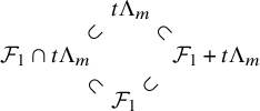
where the quotients arising from all slanted inclusions are finitely generated projective k-modules of rank 1. We can easily see that this holds for $ \mathcal {F}_1 = \Lambda '\otimes k$
. Since
$ \mathcal {F}_1 = \Lambda '\otimes k$
. Since $ t \Lambda _m$
is fixed by the action of
$ t \Lambda _m$
is fixed by the action of $ {\mathcal G}$
and the
$ {\mathcal G}$
and the $ {\mathcal G}$
-orbit
$ {\mathcal G}$
-orbit $ O_{wt}$
is closed, we can deduce that rank
$ O_{wt}$
is closed, we can deduce that rank $(t\mathcal {F}_1)=1$
if and only if
$(t\mathcal {F}_1)=1$
if and only if $\mathcal {F}_1 \in O_{wt}$
. Therefore, as in (A), we get
$\mathcal {F}_1 \in O_{wt}$
. Therefore, as in (A), we get $\mathrm {M}^{\mathrm {spl}}\otimes k = M_1 \cup M_2$
, where
$\mathrm {M}^{\mathrm {spl}}\otimes k = M_1 \cup M_2$
, where $M_2$
maps birationally to the special fiber of
$M_2$
maps birationally to the special fiber of $\mathrm {M}^{\mathrm {loc}}$
.
$\mathrm {M}^{\mathrm {loc}}$
.
Acknowledgements
We thank G. Pappas for several useful comments on a preliminary version of this article. We also thank the referees for their useful suggestions.
Competing interest
The authors have no competing interests to declare.
Financial support
The first author was supported by CRC 1442 Geometry: Deformations and Rigidity and the Excellence Cluster of the Universität Münster.


 Open access