


Introduction
Let $\mathfrak {g}$
be a simple finite-dimensional complex Lie algebra and
$\mathfrak {g}$
be a simple finite-dimensional complex Lie algebra and $\mathfrak {g}\otimes \mathbb {C}[t,t^{-1}]$
the loop algebra of
$\mathfrak {g}\otimes \mathbb {C}[t,t^{-1}]$
the loop algebra of $\mathfrak {g}$
with commutation relations
$\mathfrak {g}$
with commutation relations $[x\otimes f, y\otimes g]=[x,y]\otimes fg$
, for
$[x\otimes f, y\otimes g]=[x,y]\otimes fg$
, for $x,y\in \mathfrak {g}$
and
$x,y\in \mathfrak {g}$
and $f,g\in \mathbb {C}[t,t^{-1}]$
. In the construction of the loop algebra, we may replace the Laurent polynomial algebra
$f,g\in \mathbb {C}[t,t^{-1}]$
. In the construction of the loop algebra, we may replace the Laurent polynomial algebra $\mathbb {C}[t,t^{-1}]$
by any other commutative associative complex algebra R. In particular, if R is the algebra of regular functions over an affine scheme of finite type X, we obtain the Lie algebra of all regular maps from X to
$\mathbb {C}[t,t^{-1}]$
by any other commutative associative complex algebra R. In particular, if R is the algebra of regular functions over an affine scheme of finite type X, we obtain the Lie algebra of all regular maps from X to $\mathfrak {g}$
. If R is the ring of meromorphic functions on a Riemann surface with a fixed number of poles, we obtain a current Krichever-Novikov algebra. These algebras where introduced by Krichever and Novikov in their study of string theory in Minkowski space [Reference Krichever and Novikov16], [Reference Krichever and Novikov17] and extensively studied by many authors (cf. [Reference Schlichenmaier19] and references therein). In particular, the case of the ring of rational functions on the Riemann sphere regular everywhere except a finite number of points is relevant to the study of tensor module structures for affine Lie algebras ([Reference Kazhdan and Lusztig12], [Reference Kazhdan and Lusztig13]). The corresponding Lie algebras generalizing the untwisted affine Kac-Moody Lie algebras are called N-point algebras.
$\mathfrak {g}$
. If R is the ring of meromorphic functions on a Riemann surface with a fixed number of poles, we obtain a current Krichever-Novikov algebra. These algebras where introduced by Krichever and Novikov in their study of string theory in Minkowski space [Reference Krichever and Novikov16], [Reference Krichever and Novikov17] and extensively studied by many authors (cf. [Reference Schlichenmaier19] and references therein). In particular, the case of the ring of rational functions on the Riemann sphere regular everywhere except a finite number of points is relevant to the study of tensor module structures for affine Lie algebras ([Reference Kazhdan and Lusztig12], [Reference Kazhdan and Lusztig13]). The corresponding Lie algebras generalizing the untwisted affine Kac-Moody Lie algebras are called N-point algebras.
Denote by $\hat {{\mathcal {G}}}$
the universal central extension of
$\hat {{\mathcal {G}}}$
the universal central extension of ${\mathcal {G}}=\mathfrak {g}\otimes R$
. In [Reference Bremner3], Bremner described the center C of the universal central extension
${\mathcal {G}}=\mathfrak {g}\otimes R$
. In [Reference Bremner3], Bremner described the center C of the universal central extension $\hat {\mathcal {G}}$
of N-point algebras and determined its dimension. Also, in the case of the ring of regular functions on an elliptic curve with two points removed, the universal cocycle
$\hat {\mathcal {G}}$
of N-point algebras and determined its dimension. Also, in the case of the ring of regular functions on an elliptic curve with two points removed, the universal cocycle $\hat {\mathcal {G}}\times \hat {\mathcal {G}}\to C$
was computed.
$\hat {\mathcal {G}}\times \hat {\mathcal {G}}\to C$
was computed.
Following these results, Cox and Jurisich [Reference Cox and Jurisich6] described the universal central extension of the $3$
-point current algebra when
$3$
-point current algebra when $\mathfrak {g}=\mathfrak {sl}(2,\mathbb {C})$
and, furthermore, constructed their explicit realizations by differential operators. In [Reference Bremner4], Bremner constructed the universal central extension of the
$\mathfrak {g}=\mathfrak {sl}(2,\mathbb {C})$
and, furthermore, constructed their explicit realizations by differential operators. In [Reference Bremner4], Bremner constructed the universal central extension of the $4$
-point current algebra.
$4$
-point current algebra.
Date, Jimbo, Kashiwara and Miwa considered the universal central extension of $\mathfrak {g}\otimes \mathbb {C}[t,t^{-1},u]$
with
$\mathfrak {g}\otimes \mathbb {C}[t,t^{-1},u]$
with $u^2=(t^2-b^2)(t^2-c^2)$
,
$u^2=(t^2-b^2)(t^2-c^2)$
, $b\in \mathbb {C}\setminus \{-c,c\}$
in their study of Landau-Lifshitz equation [Reference Date, Jimbo, Kashiwara and Miwa10] (the so-called DJKM algebra). This is an example of a Krichever-Novikov algebra with genus different from zero.
$b\in \mathbb {C}\setminus \{-c,c\}$
in their study of Landau-Lifshitz equation [Reference Date, Jimbo, Kashiwara and Miwa10] (the so-called DJKM algebra). This is an example of a Krichever-Novikov algebra with genus different from zero.
The universal central extension of the DJKM algebras was described in [Reference Cox and Futorny7]. A realization of these algebras in terms of partial differential operators was constructed in [Reference Cox and Jurisich6] for $\mathfrak {g}=\mathfrak {sl}(2,\mathbb {C})$
and in [Reference Cox, Futorny and Martins8] for a general
$\mathfrak {g}=\mathfrak {sl}(2,\mathbb {C})$
and in [Reference Cox, Futorny and Martins8] for a general $\mathfrak {g}$
. A study of the universal central extension of the DJKM algebras led to the discovery of new families of orthogonal polynomials in [Reference Cox, Futorny and Tirao9], which belong to the families of associated ultraspherical polynomials. These non-classical orthogonal polynomials satisfy differential equations of fourth order. Orthogonal polynomials play an important role in mathematics and physics, particularly in the description of wave phenomena and vibrating systems [Reference Othmani, Zhang, Lü, Wang and Kamali18], the theory of random matrix ensembles [Reference König15] and other areas. It is curious to have such a connection between the universal central extensions of Krichever-Novikov algebras and associated ultraspherical polynomials. It would be interesting to know in general which orthogonal polynomials correspond to the universal central extensions of Krichever-Novikov algebras aiming to find new families of such polynomials satisfying higher-order differential equations.
$\mathfrak {g}$
. A study of the universal central extension of the DJKM algebras led to the discovery of new families of orthogonal polynomials in [Reference Cox, Futorny and Tirao9], which belong to the families of associated ultraspherical polynomials. These non-classical orthogonal polynomials satisfy differential equations of fourth order. Orthogonal polynomials play an important role in mathematics and physics, particularly in the description of wave phenomena and vibrating systems [Reference Othmani, Zhang, Lü, Wang and Kamali18], the theory of random matrix ensembles [Reference König15] and other areas. It is curious to have such a connection between the universal central extensions of Krichever-Novikov algebras and associated ultraspherical polynomials. It would be interesting to know in general which orthogonal polynomials correspond to the universal central extensions of Krichever-Novikov algebras aiming to find new families of such polynomials satisfying higher-order differential equations.
Building upon the previous research on the universal central extension of the DJKM algebras, we extend the study to the superelliptic case. The equation of a superelliptic curve is $u^m=p(t)$
, where
$u^m=p(t)$
, where $p(t)$
is a polynomial in t. The DJKM algebras correspond to the case
$p(t)$
is a polynomial in t. The DJKM algebras correspond to the case $m=2$
and
$m=2$
and $deg \, p(t)=4$
. We generalize the results of [Reference Cox, Futorny and Tirao9] for arbitrary superelliptic curve with
$deg \, p(t)=4$
. We generalize the results of [Reference Cox, Futorny and Tirao9] for arbitrary superelliptic curve with $m>2$
and
$m>2$
and $deg \, p(t)=4$
. Our analysis reveals the existence of two new families of orthogonal polynomials for each particular
$deg \, p(t)=4$
. Our analysis reveals the existence of two new families of orthogonal polynomials for each particular $m>2$
, which are the solutions of fourth-order differential equations as in the case the DJKM algebras. This is somewhat surprising as one may expect the order of differential equations to grow with m. One constructed family is identified as a family of associated ultraspherical polynomials. The other family is similar but has different initial conditions. As a result, it required an independent proof of the orthogonality.
$m>2$
, which are the solutions of fourth-order differential equations as in the case the DJKM algebras. This is somewhat surprising as one may expect the order of differential equations to grow with m. One constructed family is identified as a family of associated ultraspherical polynomials. The other family is similar but has different initial conditions. As a result, it required an independent proof of the orthogonality.
As a byproduct, we show that certain superelliptic integrals are solutions of elliptic PDEs of fourth-order (cf. Corollaries 2.2 and 2.4). This is of interest on its own since the PDEs we consider are not completely integrable and do not fall into any other class of PDEs with explicit solutions. In the cases when such explicit solutions are known, they are of importance in different areas of mathematics [Reference Ablowitz and Clarkson1] and theoretical physics [Reference Kamchatnov11].
1 Superelliptic affine Lie algebras
Let R be a ring of the form $\mathbb {C}[t,t^{-1}, u]$
, where
$\mathbb {C}[t,t^{-1}, u]$
, where $u^m\in \mathbb {C}[t]$
and
$u^m\in \mathbb {C}[t]$
and $m\geq 2$
. Thus, R has a basis consisting of
$m\geq 2$
. Thus, R has a basis consisting of $t^i$
,
$t^i$
, $t^iu$
,
$t^iu$
, $t^iu^2\dots ,t^iu^{m-1}$
for
$t^iu^2\dots ,t^iu^{m-1}$
for $i\in \mathbb {Z}$
. We will assume that
$i\in \mathbb {Z}$
. We will assume that $P(t)=\sum ^{D}_{i=0}a_it^i$
, where
$P(t)=\sum ^{D}_{i=0}a_it^i$
, where $a_D=1$
and
$a_D=1$
and $a_0,a_1$
are not both 0 and that
$a_0,a_1$
are not both 0 and that $P(t)$
has no multiple roots. The equation
$P(t)$
has no multiple roots. The equation $u^m=P(t)$
defines a superelliptic curve. Set
$u^m=P(t)$
defines a superelliptic curve. Set $R^i$
for
$R^i$
for $\mathbb {C}[t,t^{-1}]u^i$
. Then
$\mathbb {C}[t,t^{-1}]u^i$
. Then $R=R^0\oplus R^1\oplus \cdots \oplus R^{m-1}$
is a
$R=R^0\oplus R^1\oplus \cdots \oplus R^{m-1}$
is a $\mathbb {Z}/m\mathbb {Z}$
-grading.
$\mathbb {Z}/m\mathbb {Z}$
-grading.
Let $\mathfrak {g}$
be a simple finite-dimensional complex Lie algebra. The Lie algebra
$\mathfrak {g}$
be a simple finite-dimensional complex Lie algebra. The Lie algebra ${\mathcal {G}}=\mathfrak {g} \otimes R$
is an example of superelliptic loop algebras. The
${\mathcal {G}}=\mathfrak {g} \otimes R$
is an example of superelliptic loop algebras. The $\mathbb {Z}/m\mathbb {Z}$
-grading induces the structure of a
$\mathbb {Z}/m\mathbb {Z}$
-grading induces the structure of a $\mathbb {Z}/m\mathbb {Z}$
-graded Lie algebra on
$\mathbb {Z}/m\mathbb {Z}$
-graded Lie algebra on ${\mathcal {G}}$
by setting
${\mathcal {G}}$
by setting ${\mathcal {G}}^i=\mathfrak {g}\otimes R^i$
(
${\mathcal {G}}^i=\mathfrak {g}\otimes R^i$
( $i=0,1,2,\dots , m-1$
).
$i=0,1,2,\dots , m-1$
).
Let $\hat {\mathcal {G}}={\mathcal {G}}\oplus C$
be the universal central extension of
$\hat {\mathcal {G}}={\mathcal {G}}\oplus C$
be the universal central extension of ${\mathcal {G}}$
, where C is the center of
${\mathcal {G}}$
, where C is the center of $\hat {\mathcal {G}}$
. By [Reference Kassel14], the center C is linearly isomorphic to
$\hat {\mathcal {G}}$
. By [Reference Kassel14], the center C is linearly isomorphic to $\Omega _R^1/dR$
, the space of Kähler differentials of R modulo the exact differentials. Our goal is to determine a basis for
$\Omega _R^1/dR$
, the space of Kähler differentials of R modulo the exact differentials. Our goal is to determine a basis for $\Omega _R^1/dR$
.
$\Omega _R^1/dR$
.
Let $F=R\otimes R$
be the left R-module with action
$F=R\otimes R$
be the left R-module with action $f(g\otimes h)=fg\otimes h$
for
$f(g\otimes h)=fg\otimes h$
for $f, g, h\in R$
. Let K be the submodule generated by the elements
$f, g, h\in R$
. Let K be the submodule generated by the elements $1\otimes fg-f\otimes g-g\otimes f$
. Then
$1\otimes fg-f\otimes g-g\otimes f$
. Then $\Omega _R^1=F/K$
is the module of Kähler differentials. We denote the element
$\Omega _R^1=F/K$
is the module of Kähler differentials. We denote the element $f\otimes g+K$
of
$f\otimes g+K$
of $\Omega _R^1$
by
$\Omega _R^1$
by $fdg$
. We define a map
$fdg$
. We define a map $d:R\rightarrow \Omega _R^1$
by
$d:R\rightarrow \Omega _R^1$
by $d(f)=df=1\otimes f+K$
, and we denote the coset of
$d(f)=df=1\otimes f+K$
, and we denote the coset of $fdg$
modulo
$fdg$
modulo $dR$
by
$dR$
by $\overline {fdg}$
. We have
$\overline {fdg}$
. We have
 $$ \begin{align} [x\otimes f, y\otimes g]=[xy]\otimes fg+(x,y)\overline{fdg},&& [x\otimes f,\omega]=0,&& [\omega, \omega']=0, \end{align} $$
where $x,y\in \mathfrak {g}$
,
$x,y\in \mathfrak {g}$
, $f,g\in R$
and
$f,g\in R$
and $\omega , \omega ' \in \Omega _R^1/dR$
; here,
$\omega , \omega ' \in \Omega _R^1/dR$
; here, $(x,y)$
denotes the Killing form on
$(x,y)$
denotes the Killing form on $\mathfrak {g}$
.
$\mathfrak {g}$
.
The elements $t^iu^k\otimes t^ju^l$
, with
$t^iu^k\otimes t^ju^l$
, with $i,j\in \mathbb {Z}$
and
$i,j\in \mathbb {Z}$
and $k,l\in \{0,1,\dots , m-1\}$
form a basis of
$k,l\in \{0,1,\dots , m-1\}$
form a basis of $R\otimes R$
. The following result is fundamental to the description of the universal central extension for
$R\otimes R$
. The following result is fundamental to the description of the universal central extension for $R=\mathbb {C}[t,t^{-1},u|\,\, u^m=P(t)]$
.
$R=\mathbb {C}[t,t^{-1},u|\,\, u^m=P(t)]$
.
Theorem 1.1 ([Reference Albino dos Santos2], Theorem 2.4).
The following elements form a basis of $\Omega _R^1/dR$
:
$\Omega _R^1/dR$
:
 $$ \begin{align*}\overline{t^{-1}dt}, \, \overline{t^{-1}u^ldt}, \, \dots, \, \overline{t^{-D}u^ldt},\end{align*} $$
where $l\in \{1,2,\dots ,m-1\}$
and we omit
$l\in \{1,2,\dots ,m-1\}$
and we omit $\overline {t^{-D}u^ldt}$
if
$\overline {t^{-D}u^ldt}$
if $a_0=0$
.
$a_0=0$
.
We have the following relation between the basis elements:
Proposition 1.2 ([Reference Cox and Futorny7], Lemma 2.0.2).
If $u^m=P(t)$
and
$u^m=P(t)$
and $R=[t,t^{-1},u|\,\, u^m=P(t)\,\, ]$
, then in
$R=[t,t^{-1},u|\,\, u^m=P(t)\,\, ]$
, then in $\Omega _R^1/dR$
, one has
$\Omega _R^1/dR$
, one has
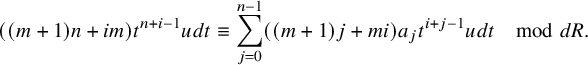 $$ \begin{align} ((m+1)n+im)t^{n+i-1}udt\equiv\sum_{j=0}^{n-1}((m+1)j+mi)a_jt^{i+j-1}udt\quad \mod{dR}. \end{align} $$
This allows to describe the universal central extension of the superelliptic algebra.
Let us define the sequence of polynomials in $D+3$
parameters
$D+3$
parameters $P_{m,n,l}(a_{0},a_{1},\dots ,a_{D-1}):=P_{n}$
for
$P_{m,n,l}(a_{0},a_{1},\dots ,a_{D-1}):=P_{n}$
for $n\geq -D$
,
$n\geq -D$
, $m, l\in \mathbb {Z}_+$
and
$m, l\in \mathbb {Z}_+$
and $a_{0},a_{1},\dots ,a_{D-1}\in \mathbb {C}$
as follows:
$a_{0},a_{1},\dots ,a_{D-1}\in \mathbb {C}$
as follows:
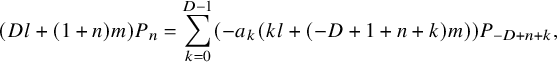 $$ \begin{align} (Dl+(1+n)m)P_n=\sum_{k=0}^{D-1}\left(-a_k\left(kl+(-D+1+n+k)m\right) \right) P_{-D+n+k}, \end{align} $$
with initial condition
 $$ \begin{align} P_{-D}=t^{-D}u^ldt, \, P_{-D+1}=t^{-D+1}u^ldt, \, \dots, \, P_{-1}=t^{-1}u^ldt. \end{align} $$
Then $P_n= t^{n}u^ldt$
for all
$P_n= t^{n}u^ldt$
for all $n\geq 0$
.
$n\geq 0$
.
If $a_0\neq 0$
, we define the sequence of polynomials in
$a_0\neq 0$
, we define the sequence of polynomials in $D+3$
parameters
$D+3$
parameters $Q_{m,n,l}(a_{0},a_{1},\dots ,a_{D-1}):=Q_{n}$
for
$Q_{m,n,l}(a_{0},a_{1},\dots ,a_{D-1}):=Q_{n}$
for $n\leq -D-1$
,
$n\leq -D-1$
, $m, l\in \mathbb {Z}_+$
and
$m, l\in \mathbb {Z}_+$
and $a_{0},a_{1},\dots ,a_{D-1}\in \mathbb {C}$
as follows:
$a_{0},a_{1},\dots ,a_{D-1}\in \mathbb {C}$
as follows:
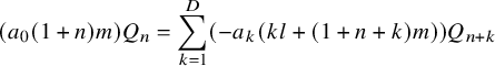 $$ \begin{align} (a_0(1+n)m)Q_n=\sum_{k=1}^{D}\left(-a_k\left(kl+(1+n+k)m\right) \right) Q_{n+k} \end{align} $$
with initial conditions
 $$ \begin{align} Q_{-D}=t^{-D}u^ldt, \, Q_{-D+1}=t^{-D+1}u^ldt, \, \dots, \, Q_{-1}=t^{-1}u^ldt. \end{align} $$
Then $Q_n=t^{n}u^ldt$
for
$Q_n=t^{n}u^ldt$
for $n\leq -D-1$
.
$n\leq -D-1$
.
If $a_0=0$
, we define the sequence of polynomials in
$a_0=0$
, we define the sequence of polynomials in $D+3$
parameters
$D+3$
parameters $R_{m,n,l}(a_{0},a_{1},\dots ,a_{D-1}):=R_{n}$
for
$R_{m,n,l}(a_{0},a_{1},\dots ,a_{D-1}):=R_{n}$
for $n\leq -D-1$
,
$n\leq -D-1$
, $m, l\in \mathbb {Z}_+$
and
$m, l\in \mathbb {Z}_+$
and $a_{0},a_{1},\dots ,a_{D-1}\in \mathbb {C}$
as follows:
$a_{0},a_{1},\dots ,a_{D-1}\in \mathbb {C}$
as follows:
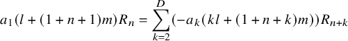 $$ \begin{align} a_1(l+(1+n+1)m)R_n=\sum_{k=2}^{D}\left(-a_k\left(kl+(1+n+k)m\right) \right) R_{n+k} \end{align} $$
with initial condition
 $$ \begin{align} R_{-D+1}=t^{-D+1}u^ldt, \, R_{-D+2}=t^{-D+2}u^ldt, \, \dots, \, R_{-1}=t^{-1}u^ldt. \end{align} $$
We see that $R_n=t^{n}u^ldt$
,
$R_n=t^{n}u^ldt$
, $n\leq -D-1$
.
$n\leq -D-1$
.
Set
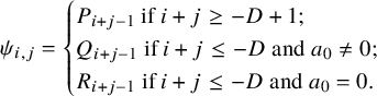 $$ \begin{align} \psi_{i,j}= \begin{cases} P_{i+j-1} \textrm{ if } i+j\geq -D+1;\\ Q_{i+j-1} \textrm{ if } i+j\leq -D \textrm{ and } a_0\neq0;\\ R_{i+j-1} \textrm{ if } i+j\leq -D\textrm{ and } a_0=0. \end{cases} \end{align} $$
Then $ t^{i}u^ld(t^j) = j \psi _{i,j}$
[[Reference Albino dos Santos2], Proposition 3.4].
$ t^{i}u^ld(t^j) = j \psi _{i,j}$
[[Reference Albino dos Santos2], Proposition 3.4].
We have the following description of the Lie algebra structure on $\hat {\mathcal {G}}$
. Set
$\hat {\mathcal {G}}$
. Set
 $$ \begin{align} \omega_0=\overline{t^{-1}dt} \textrm{ and } \omega_{ij}=\overline{t^{i}u^jdt} \textrm{ for } j\neq 0. \end{align} $$
Theorem 1.3 ([Reference Albino dos Santos2], Theorem 3.5).
The superelliptic affine Lie algebra $\hat {\mathcal {G}}$
has a
$\hat {\mathcal {G}}$
has a $\mathbb {Z}/m\mathbb {Z}$
-grading in which
$\mathbb {Z}/m\mathbb {Z}$
-grading in which
 $$ \begin{align*} \hat{\mathcal{G}}^0=\mathfrak{g}\otimes\mathbb{C}[t,t^{-1}]\oplus \mathbb{C}\omega_0,&& \hat{\mathcal{G}}^l=\mathfrak{g}\otimes\mathbb{C}[t,t^{-1}]u^l\bigoplus_{n=1}^D \mathbb{C}\omega_{-n,l}. \end{align*} $$
The subalgebra $\hat {\mathcal {G}}^0$
is an untwisted affine Kac-Moody Lie algebra with commutation relations
$\hat {\mathcal {G}}^0$
is an untwisted affine Kac-Moody Lie algebra with commutation relations
 $$ \begin{align*} [x\otimes t^i,y\otimes t^j]=[x,y]\otimes t^{i+j}\oplus \delta_{i+j,0}(x,y)j\omega_0. \end{align*} $$
The commutation relations in $\mathcal {\hat {G}}$
are
$\mathcal {\hat {G}}$
are
 $$ \begin{align*} [x\otimes t^iu^{l_1},y\otimes t^ju^{l_2}]=[x,y]\otimes (t^{i+j}u^{l_1+l_2})+(x,y)\left(\frac{jl_1-il_2}{l_1+l_2}\right) \omega_{i+j-1,l_1+l_2}, \end{align*} $$
if $l_1+l_2\leq m-1$
. When
$l_1+l_2\leq m-1$
. When $l_1+l_2>m-1$
,
$l_1+l_2>m-1$
,
 $$ \begin{align*} {}[x\otimes t^iu^{l_1},y\otimes t^ju^{l_2}]=[x,y]\otimes \left(\sum_{k=0}^D a_kt^{i+j+k}u^{l_1+l_2-m}\right)+(x,y)\left(\frac{jl_1-il_2}{l_1+l_2}\right) \omega_{i+j-1,l_1+l_2}. \end{align*} $$
The subspace $\mathcal {\hat {G}}^l$
is a
$\mathcal {\hat {G}}^l$
is a $\mathcal {\hat {G}}^0$
-module with
$\mathcal {\hat {G}}^0$
-module with
 $$ \begin{align} [x\otimes t^iu^n,y\otimes t^j]=&[x,y]\otimes (t^{i+j}u^{n+1})+(x,y)j\psi_{i,j}. \end{align} $$
In this paper, we will consider the superelliptic affine Lie algebras with the polynomial relation
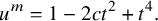 $$ \begin{align*}u^m=1-2 c t^2+t^4.\end{align*} $$
In this case, letting $k=i+3$
, the recursion relation (1.2) becomes
$k=i+3$
, the recursion relation (1.2) becomes
 $$ \begin{align*} (4+m+k m) \overline{t^k \text{udt}}=-(k-3) m \overline{t^{-4+k} \text{udt}}+2 c (2+(k-1) m) \overline{t^{-2+k} \text{udt}}. \end{align*} $$
Consider a family $P_k:=P_k(c)$
of polynomials in c satisfying the recursion relation
$P_k:=P_k(c)$
of polynomials in c satisfying the recursion relation
 $$ \begin{align} (k m+m+4) P_k(c)=2 c ((k-1) m+2) P_{k-2}(c)-(k-3) m P_{k-4}(c) \end{align} $$
for $k\geq 0$
. Set
$k\geq 0$
. Set
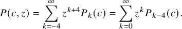 $$ \begin{align*} P(c,z)=\sum _{k=-4}^{\infty } z^{k+4} P_k(c)=\sum _{k=0}^{\infty } z^{k} P_{k-4}(c). \end{align*} $$
After a straightforward rearrangement of terms, we have
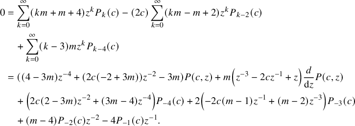 $$ \begin{align*} 0&=\sum _{k=0}^{\infty } (k m+m+4) z^k P_k(c)-(2 c) \sum _{k=0}^{\infty } (k m-m+2) z^k P_{k-2}(c) \\& \quad +\sum _{k=0}^{\infty } (k-3) m z^k P_{k-4}(c)\\&= ((4 - 3 m)z^{-4} + (2 c (-2 + 3 m)) z^{-2} - 3 m) P(c,z) + m \left(z^{-3}-2cz^{-1}+z \right)\frac{d}{\textrm{d}z} P(c,z) \\& \quad + \left(2 c (2-3 m) z^{-2}+(3 m-4)z^{-4}\right)P_{-4}(c) + 2 \left(-2 c (m-1) z^{-1}+(m-2)z^{-3}\right)P_{-3}(c) \\& \quad + (m-4) P_{-2}(c)z^{-2}-4 P_{-1}(c) z^{-1}. \end{align*} $$
Hence, $P(c, z)$
satisfies the differential equation
$P(c, z)$
satisfies the differential equation
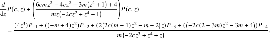 $$ \begin{align} &\frac{d}{\textrm{d}z}P(c,z)+\left(\frac{6 c m z^2-4 c z^2-3 m \left(z^4+1\right)+4}{m z \left(-2 c z^2+z^4+1\right)}\right)P(c,z) \nonumber \\& \quad =\frac{(4 z^3) P_{-1} + ((-m+4)z^2) P_{-2}+ (2\left(2 c (m-1) z^2-m+2\right)z) P_{-3} +({ \left(-2 c (2-3 m) z^2-3 m+4\right)})P_{-4}}{m \left(-2 c z^3+z^4+z\right)}. \end{align} $$
It has an integrating factor
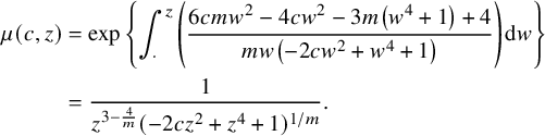 $$ \begin{align*} \mu(c,z)&=\exp{\left\{\int_{\cdot}^z \left(\frac{6 c m w^2-4 c w^2-3 m \left(w^4+1\right)+4}{m w \left(-2 c w^2+w^4+1\right)}\right) \textrm{d}w\right\}} \\ &= \frac{1}{z^{3-\frac{4}{m}}(-2 c z^2+z^4+1)^{1/m}}. \end{align*} $$
Now, we consider different cases depending on the initial conditions.
1.1 Superelliptic case 1
Assume that $P_{-3}=P_{-2}=P_{-1}=0$
and
$P_{-3}=P_{-2}=P_{-1}=0$
and $P_{-4}=1$
, and denote the generating function in this case by
$P_{-4}=1$
, and denote the generating function in this case by $ P_{-4}(c,z)$
. Then
$ P_{-4}(c,z)$
. Then
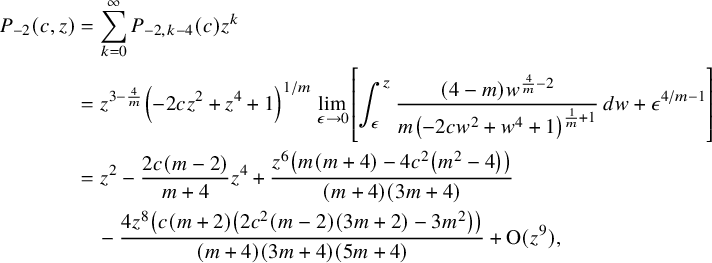
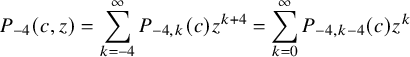 $$ \begin{align*} P_{-4}(c,z)=\sum _{k=-4}^{\infty } P_{-4,k}(c)z^{k+4} =\sum _{k=0}^{\infty }P_{-4,k-4}(c) z^{k} \end{align*} $$
can be written in terms of a superelliptic integral
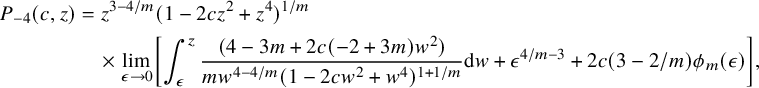 $$ \begin{align} P_{-4}(c,z)&=z^{3-4/m} (1-2 c z^2+z^4)^{1/m}\nonumber\\&\quad \times\lim_{\epsilon\to 0}\left[\int_{\epsilon}^{z} \frac{(4-3 m+2 c(-2+3 m) w^2)}{mw^{4-4/m} (1-2 c w^2+w^4)^{1+1/m}} \textrm{d}w+\epsilon^{4/m-3}+2c(3-2/m)\phi_m(\epsilon)\right], \end{align} $$
where
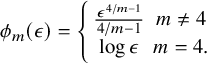 $$\begin{align*}\phi_m(\epsilon)= \left\{ \begin{array}{cc} \frac{\epsilon^{4/m-1}}{4/m-1} & m\neq 4\\ \log{\epsilon} & m=4. \end{array} \right. \end{align*}$$
Remark 1.15. The correction term inside of the limit $\epsilon \to 0$
in the formula (1.14) is necessary to ensure finiteness of the limit.
$\epsilon \to 0$
in the formula (1.14) is necessary to ensure finiteness of the limit.
1.2 Superelliptic case 2
Suppose now that $P_{-3}=P_{-4}=P_{-1}=0$
and
$P_{-3}=P_{-4}=P_{-1}=0$
and $P_{-2}=1$
. Then we arrive to the generating function
$P_{-2}=1$
. Then we arrive to the generating function
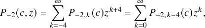 $$ \begin{align*} P_{-2}(c,z)=\sum _{k=-4}^{\infty } P_{-2,k}(c)z^{k+4} =\sum _{k=0}^{\infty }P_{-2,k-4}(c) z^{k}, \end{align*} $$
which is defined in terms of a superelliptic integral
 $$ \begin{align*} P_{-2}(c,z)=z^{3-4/m} (1-2 c z^2+z^4)^{1/m}\lim_{\epsilon\to 0}\left[\int_{\epsilon}^{z} \frac{(4 - m) }{m w^{2-4/m} (1-2 c w^2+w^4)^{1+1/m}} \textrm{d}w+\epsilon^{4/m-1}\right]. \end{align*} $$
1.3 Gegenbauer case 3
If we take $P_{-1}(c) = 1$
, and
$P_{-1}(c) = 1$
, and $P_{-2}(c) = P_{-3}(c) = P_{-4}(c) = 0$
and set
$P_{-2}(c) = P_{-3}(c) = P_{-4}(c) = 0$
and set $P_{-1}(c,z)=\sum _{n\geq 0}P_{-1,n-4}z^n$
, then
$P_{-1}(c,z)=\sum _{n\geq 0}P_{-1,n-4}z^n$
, then
 $$ \begin{align*} P_{-1}(c,z)=\frac{\left(4 z^{3-\frac{4}{m}} \left(-2 c z^2+z^4+1\right)^{1/m}\right)}{m} \sum_{n=0}^{\infty} \frac{z^{\frac{4}{m}+2n} Q_n^{\left(1+\frac{1}{m}\right)}(c)}{\frac{4}{m}+2 n}, \end{align*} $$
where $Q_n^{\left (1+\frac {1}{m}\right )}(c)$
is the n-th Gegenbauer polynomial.
$Q_n^{\left (1+\frac {1}{m}\right )}(c)$
is the n-th Gegenbauer polynomial.
1.4 Gegenbauer case 4
If we take $P_{-3}(c) = 1$
, and
$P_{-3}(c) = 1$
, and $P_{-1}(c) = P_{-2}(c) = P_{-4}(c) = 0$
and set
$P_{-1}(c) = P_{-2}(c) = P_{-4}(c) = 0$
and set $P_{-3}(c,z)=\sum _{n\geq 0}P_{-1,n-4}z^n$
, then
$P_{-3}(c,z)=\sum _{n\geq 0}P_{-1,n-4}z^n$
, then
 $$ \begin{align*} P_{-3}(c,z)=\frac{\left(z^{3-\frac{4}{m}} \left(-2 c z^2+z^4+1\right)^{1/m}\right)}{2} \sum _{n=0}^{\infty } z^{\frac{4}{m}+2 n} Q_n^{\left(1+\frac{1}{m}\right)}(c) \left(\frac{m-2}{z^2 (m (n-1)+2)}-\frac{2 c (m-1)}{m n+2}\right). \end{align*} $$
We will see in the last section that the family of polynomials described in the superelliptic case 1 is an example of associated ultraspherical polynomials.
2 Orthogonal polynomials in superelliptic cases
2.1 Superelliptic type 1
Let us reindex the polynomials $P_{-4,n}$
as follows:
$P_{-4,n}$
as follows:
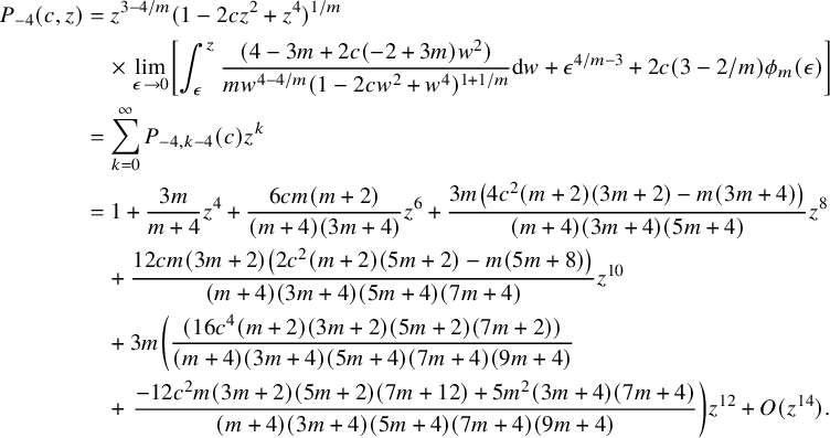 $$ \begin{align*} P_{-4}(c,z)&=z^{3-4/m} (1-2 c z^2+z^4)^{1/m}\\& \quad \times\lim_{\epsilon\to 0}\left[\int_{\epsilon}^{z} \frac{(4-3 m+2 c(-2+3 m) w^2)}{mw^{4-4/m} (1-2 c w^2+w^4)^{1+1/m}} \textrm{d}w+\epsilon^{4/m-3}+2c(3-2/m)\phi_m(\epsilon)\right]\\&= \sum _{k=0}^{\infty }P_{-4,k-4}(c) z^{k}\\&= 1+\frac{3 m }{m+4}z^4+\frac{6 c m (m+2) }{(m+4) (3 m+4)}z^6 +\frac{3 m \left(4 c^2 (m+2) (3 m+2)-m (3 m+4)\right)}{(m+4) (3 m+4) (5 m+4)}z^8\\& \quad +\frac{12 c m (3 m+2) \left(2 c^2 (m+2) (5 m+2)-m (5 m+8)\right)}{(m+4) (3 m+4) (5 m+4) (7 m+4)}z^{10}\\& \quad +3 m\left(\frac{ (16 c^4 (m+2) (3 m+2) (5 m+2) (7 m+2))}{(m+4) (3 m+4) (5 m+4) (7 m+4) (9 m+4)}\right. \\& \quad +\left.\frac{-12 c^2 m (3 m+2) (5 m+2) (7 m+12)+5 m^2 (3 m+4) (7 m+4)}{(m+4) (3 m+4) (5 m+4) (7 m+4) (9 m+4)}\right)z^{12} + O(z^{14}). \end{align*} $$
The first nonzero polynomials are
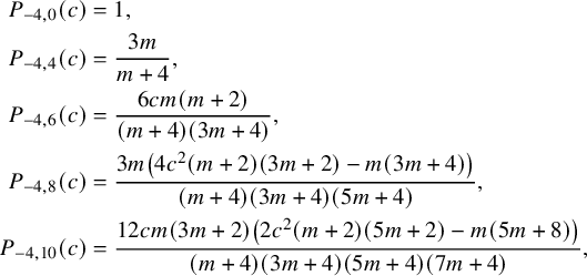 $$ \begin{align*} P_{-4,0}(c) &= 1,\\P_{-4,4}(c)&=\frac{3 m }{m+4}, \\P_{-4,6}(c)&=\frac{6 c m (m+2) }{(m+4) (3 m+4)}, \\P_{-4,8}(c)&=\frac{3 m \left(4 c^2 (m+2) (3 m+2)-m (3 m+4)\right)}{(m+4) (3 m+4) (5 m+4)}, \\P_{-4,10}(c)&=\frac{12 c m (3 m+2) \left(2 c^2 (m+2) (5 m+2)-m (5 m+8)\right)}{(m+4) (3 m+4) (5 m+4) (7 m+4)}, \end{align*} $$
and $P_n(c)=P_{-4,n}(c)$
satisfies the recursion
$P_n(c)=P_{-4,n}(c)$
satisfies the recursion
 $$ \begin{align} 0=(2 c ((k-1) m+2)) P_{k+2}(c)-(k m+m+4) P_{k+4}(c)-((k-3) m) P_k(c). \end{align} $$
Our main result is the following theorem which generalizes [[Reference Cox, Futorny and Tirao9], Theorem 3.1.1].
Theorem 2.1. The polynomials $P_n=P_{-4,n}$
satisfy the following fourth-order linear differential equation:
$P_n=P_{-4,n}$
satisfy the following fourth-order linear differential equation:
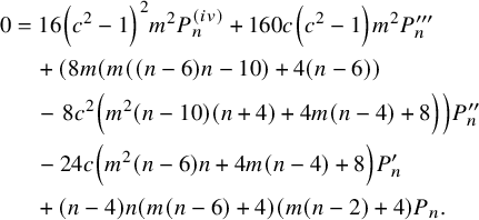 $$ \begin{align} 0&=16 \left(c^2-1\right)^2 m^2 P^ {(iv)}_n +160 c \left(c^2-1\right) m^2 P^{\prime\prime\prime}_n \nonumber\\& \quad +\left(8 m (m ((n-6) n-10)+4 (n-6))\right.\nonumber\\& \quad -\left.8 c^2 \left(m^2 (n-10) (n+4)+4 m (n-4)+8\right)\right) P^{\prime\prime}_n \nonumber\\& \quad -24 c \left(m^2 (n-6) n+4 m (n-4)+8\right) P^{\prime}_n \nonumber\\& \quad +(n-4) n (m (n-6)+4) (m (n-2)+4) P_n. \end{align} $$
Proof. See Appendix.
Denote $v:=\ln z$
and, consequently,
$v:=\ln z$
and, consequently, $\frac {\partial }{\partial v}=z\frac {\partial }{\partial z}$
.
$\frac {\partial }{\partial v}=z\frac {\partial }{\partial z}$
.
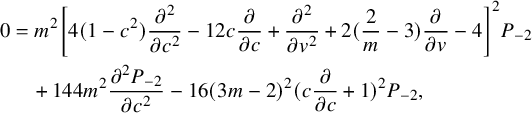
Corollary 2.2. The generating function $P_{-4}=P_{-4}(c,z)$
satisfies the following linear PDE of fourth order:
$P_{-4}=P_{-4}(c,z)$
satisfies the following linear PDE of fourth order:
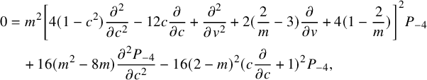 $$ \begin{align} 0&= m^2\left[4(1-c^2)\frac{\partial^2 }{\partial c^2}-12 c\frac{\partial }{\partial c}+\frac{\partial^2 }{\partial v^2} +2 (\frac{2}{m}-3)\frac{\partial }{\partial v}+4(1-\frac{2}{m})\right]^2 P_{-4}\notag\\&\quad +16(m^2-8m)\frac{\partial^2 P_{-4}}{\partial c^2}-16(2-m)^2(c\frac{\partial }{\partial c}+1)^2P_{-4}, \end{align} $$
with $(c,z)\in (-1,1)\times (0,1)$
and with the following boundary conditions:
$(c,z)\in (-1,1)\times (0,1)$
and with the following boundary conditions:
 $$ \begin{align} P_{-4}(c,0)=1, \frac{\partial P_{-4}}{\partial z}(c,0)=\frac{\partial^2 P_{-4}}{\partial z^2}(c,0)=\frac{\partial^3 P_{-4}}{\partial z^3}(c,0)=0. \end{align} $$
Proof. It follows from (1.14) that $P_{-4}$
is an analytic function represented by the series
$P_{-4}$
is an analytic function represented by the series $P_{-4}(c,z)=\sum \limits _{n=0}^{\infty } P_{-4,n}(c)z^n$
(in some ball of small radius). Hence, by Theorem 2.1 and some elementary algebraic calculations,
$P_{-4}(c,z)=\sum \limits _{n=0}^{\infty } P_{-4,n}(c)z^n$
(in some ball of small radius). Hence, by Theorem 2.1 and some elementary algebraic calculations, $P_{-4}$
satisfies the linear PDE (2.3) in the ball. By the uniqueness of analytic continuation, it satisfies the PDE (2.3) in the domain
$P_{-4}$
satisfies the linear PDE (2.3) in the ball. By the uniqueness of analytic continuation, it satisfies the PDE (2.3) in the domain $(-1,1)\times (0,1)$
. The boundary conditions (2.4) immediately follow from the definition of
$(-1,1)\times (0,1)$
. The boundary conditions (2.4) immediately follow from the definition of $P_{-4}$
.
$P_{-4}$
.
Remark 2.5. Boundary conditions for $P_{-4}$
on other parts of the boundary of the domain
$P_{-4}$
on other parts of the boundary of the domain $[-1,1]\times [0,1]$
can be explicitly calculated using formula (1.14).
$[-1,1]\times [0,1]$
can be explicitly calculated using formula (1.14).
2.2 Superelliptic type 2
Now we consider the second family of polynomials $P_{-2,n}$
. We have
$P_{-2,n}$
. We have
 $$ \begin{align*} P_{-2}(c,z)&=\sum _{k=0}^{\infty }P_{-2,k-4}(c) z^{k} \\&=z^{3-\frac{4}{m}} \left(-2 c z^2+z^4+1\right)^{1/m} \lim_{\epsilon\to 0}\left[\int_{\epsilon}^{z} \frac{(4-m) w^{\frac{4}{m}-2}}{m \left(-2 c w^2+w^4+1\right)^{\frac{1}{m}+1}} \, dw +\epsilon^{4/m-1}\right] \\&=z^2-\frac{2 c (m-2)}{m+4}z^4+\frac{z^6 \left(m (m+4)-4 c^2 \left(m^2-4\right)\right)}{(m+4) (3 m+4)}\\& \quad -\frac{4 z^8 \left(c (m+2) \left(2 c^2 (m-2) (3 m+2)-3 m^2\right)\right)}{(m+4) (3 m+4) (5 m+4)}+\textrm{O}(z^9), \end{align*} $$
and the polynomials $P_{-2,n}(c)$
satisfy the following recursion:
$P_{-2,n}(c)$
satisfy the following recursion:
 $$ \begin{align} 0=2 c (km-m+2) P_{-2,k+2}(c)-(k m+m+4) P_{-2,k+4}(c)-(km-3m) P_{-2,k}(c). \end{align} $$
In particular, the first nonzero polynomials of the sequence are
 $$ \begin{align*} P_{-2,2}(c)&=1, \\P_{-2,4}(c)&=-\frac{2 c (m-2)}{m+4}, \\P_{-2,6}(c)&=\frac{m (m+4)-4 c^2 \left(m^2-4\right)}{(m+4) (3 m+4)}, \\P_{-2,8}(c)&=-\frac{4 c (m+2) \left(2 c^2 (m-2) (3 m+2)-3 m^2\right)}{(m+4) (3 m+4) (5 m+4)}. \end{align*} $$
Theorem 2.3. The polynomials $P_n=P_{-2,n}(c)$
satisfy the following fourth-order linear differential equation:
$P_n=P_{-2,n}(c)$
satisfy the following fourth-order linear differential equation:
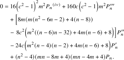 $$ \begin{align} 0&=16 \left(c^2-1\right)^2 m^2 P_n{}^{(iv)}+160 c \left(c^2-1\right) m^2 P^{\prime\prime\prime}_n\nonumber\\& \quad +\Big[8 m (m (n^2-6n-2)+4 (n-8))\nonumber\\& \quad -\left.8 c^2 \left(m^2 ((n-6) n-32)+4 m (n-6)+8\right)\right] P^{\prime\prime}_n\nonumber\\& \quad -24 c \left(m^2 (n-4) (n-2)+4 m (n-6)+8\right) P^{\prime}_n\nonumber\\& \quad +(n^2-4) (m n-8m+4) (m n-4m+4) P_n. \end{align} $$
Corollary 2.4. Generating function $P_{-2}=P_{-2}(c,z)$
satisfies the following linear PDE of fourth order:
$P_{-2}=P_{-2}(c,z)$
satisfies the following linear PDE of fourth order:
 $$ \begin{align} 0&=m^2\left[4(1-c^2)\frac{\partial^2 }{\partial c^2}-12 c\frac{\partial }{\partial c}+\frac{\partial^2 }{\partial v^2} +2 (\frac{2}{m}-3)\frac{\partial }{\partial v}-4\right]^2 P_{-2}\notag\\&\quad +144 m^2\frac{\partial^2 P_{-2}}{\partial c^2}-16(3m-2)^2(c\frac{\partial }{\partial c}+1)^2 P_{-2}, \end{align} $$
(where $v=\ln z$
,
$v=\ln z$
, $\frac {\partial }{\partial v}=z\frac {\partial }{\partial z}$
) with
$\frac {\partial }{\partial v}=z\frac {\partial }{\partial z}$
) with $(c,z)\in (-1,1)\times (0,1)$
and with the following boundary conditions:
$(c,z)\in (-1,1)\times (0,1)$
and with the following boundary conditions:
 $$ \begin{align} \frac{\partial^2 P_{-2}}{\partial z^2}(c,0)=1, P_{-2}(c,0)=\frac{\partial P_{-2}}{\partial z}(c,0)=\frac{\partial^3 P_{-2}}{\partial z^3}(c,0)=0. \end{align} $$
Proof. The proof is analogous to the proof of Corollary 2.2.
3 Uniqueness of solutions
Let us check now if the differential equations (2.2) and (2.7) have other polynomial solutions. The argument below was suggested by A. Shyndyapin.
Clearly, if $\{P_n\}$
is a family of polynomials satisfying (2.2) (respectively, (2.7)), then for any choice of nonzero scalars
$\{P_n\}$
is a family of polynomials satisfying (2.2) (respectively, (2.7)), then for any choice of nonzero scalars $\lambda _n\in \mathbb {C}$
, the family
$\lambda _n\in \mathbb {C}$
, the family $\{\lambda _n P_n\}$
also satisfies (2.2) (respectively, (2.7)). We will call such families of polynomials equivalent. Also, we will ignore the families of polynomials obtained by zeroing some members of the family.
$\{\lambda _n P_n\}$
also satisfies (2.2) (respectively, (2.7)). We will call such families of polynomials equivalent. Also, we will ignore the families of polynomials obtained by zeroing some members of the family.
Consider first the equation (2.2) and assume that
 $$ \begin{align*}Q_n=\sum\limits_{i=0}^{r(n)} \alpha_i(n) c^i\end{align*} $$
is its polynomial solution. We will simply write r for $r(n)$
and
$r(n)$
and $\alpha _i$
for
$\alpha _i$
for $\alpha _i(n)$
. After the substitution in (2.2), we obtain
$\alpha _i(n)$
. After the substitution in (2.2), we obtain
 $$ \begin{align*} \sum _{i=0}^r &((2 i-n+4) (2 i+n) (m (2 i-n+6)-4) (m (2 i+n-2)+4))\alpha_ic^{i}\\ &+(-8 (i-1) i m \left(m \left(4 i^2-(n-6) n-6\right)-4 (n-6)\right))\alpha_ic^{i-2}\\ &+(16 (i-3) (i-2) (i-1) i m^2)\alpha_ic^{i-4}=0, \end{align*} $$
which is equivalent to the following system of linear equations:
 $$ \begin{align} &[(2 i-n+4) (2 i+n) (m (2 i-n+6)-4) (m (2 i+n-2)+4)]\alpha_i\nonumber\\& \quad +[-8 (i+1) (i+2) m (m (4 i (i+4)-(n-6) n+10)-4 (n-6))]\alpha_{i+2}\\& \quad +[16 (i+1) (i+2) (i+3) (i+4) m^2]]\alpha_{i+4}=0,\,\,\,\,\, i=0,1, \ldots, r. \nonumber \end{align} $$
Here $\alpha _s$
is assumed to be zero if
$\alpha _s$
is assumed to be zero if $s>r$
. The coefficient matrix of the system is upper triangular with
$s>r$
. The coefficient matrix of the system is upper triangular with
 $$ \begin{align*}(2 i-n+4) (2 i+n) (m (2 i-n+6)-4) (m (2 i+n-2)+4), \,\, i=0, \ldots, r\end{align*} $$
on the diagonal. Hence, for each n, the solution of the system is unique and trivial if $(2 i-n+4) (m (2 i-n+6)-4)\neq 0$
for all
$(2 i-n+4) (m (2 i-n+6)-4)\neq 0$
for all $i=0,1, \ldots , r$
. Suppose
$i=0,1, \ldots , r$
. Suppose $(2 i-n+4) (m (2 i-n+6)-4)= 0$
. First consider the case
$(2 i-n+4) (m (2 i-n+6)-4)= 0$
. First consider the case $m>4$
. Then we must have
$m>4$
. Then we must have $2i-n+4=0$
. From (3.1), we get that
$2i-n+4=0$
. From (3.1), we get that $Q_{2k+1}=0$
for all
$Q_{2k+1}=0$
for all $k>0$
, and
$k>0$
, and $Q_{2k}$
is defined uniquely up to a scalar for each
$Q_{2k}$
is defined uniquely up to a scalar for each $k>1$
. The degree of
$k>1$
. The degree of $Q_{2k}$
is
$Q_{2k}$
is $\geq k-2$
. Now, if
$\geq k-2$
. Now, if $m=4$
, then either
$m=4$
, then either $i=\frac {n}{2}-2$
or
$i=\frac {n}{2}-2$
or $i=\frac {n+1}{2}-3$
. Therefore,
$i=\frac {n+1}{2}-3$
. Therefore, $Q_{2k}$
is defined uniquely up to a scalar as a polynomial of degree
$Q_{2k}$
is defined uniquely up to a scalar as a polynomial of degree $\geq k-2$
,
$\geq k-2$
, $Q_1=Q_3=0$
and
$Q_1=Q_3=0$
and $Q_{2k+1}$
is defined uniquely up to a scalar as a polynomial of degree
$Q_{2k+1}$
is defined uniquely up to a scalar as a polynomial of degree $\geq k-2$
for each
$\geq k-2$
for each $k\geq 2$
.
$k\geq 2$
.
Consider now the equation (2.7). Arguing as above, we come a linear system on the coefficients of the polynomial solution $Q_n$
. The matrix of this system is again upper triangular with diagonal entries
$Q_n$
. The matrix of this system is again upper triangular with diagonal entries
 $$ \begin{align*}\left(4 (i+1)^2-n^2\right) (m (2 i-n+8)-4) (m (2 i+n-4)+4),\,\, i=0, \ldots, r.\end{align*} $$
Assume that $\left (4 (i+1)^2-n^2\right ) (m (2 i-n+8)-4) (m (2 i+n-4)+4)=0$
. If
$\left (4 (i+1)^2-n^2\right ) (m (2 i-n+8)-4) (m (2 i+n-4)+4)=0$
. If $m>4$
, then
$m>4$
, then $Q_{2k+1}=0$
for all
$Q_{2k+1}=0$
for all $k> 0$
, and
$k> 0$
, and $Q_{2k}$
is defined uniquely up to a scalar for each
$Q_{2k}$
is defined uniquely up to a scalar for each $k> 1$
, while
$k> 1$
, while $Q_2=0$
. The degree of
$Q_2=0$
. The degree of $Q_{2k}$
is
$Q_{2k}$
is $\geq k-2$
. Suppose now that
$\geq k-2$
. Suppose now that $m=4$
and
$m=4$
and $n>1$
. Then either
$n>1$
. Then either $i=\frac {n}{2}-1$
or
$i=\frac {n}{2}-1$
or $i=\frac {n+1}{2}-3$
. Therefore,
$i=\frac {n+1}{2}-3$
. Therefore, $Q_{2k}$
is defined uniquely up to a scalar as a polynomial of degree
$Q_{2k}$
is defined uniquely up to a scalar as a polynomial of degree $\geq k-2$
,
$\geq k-2$
, $Q_3=Q_5=0$
, and
$Q_3=Q_5=0$
, and $Q_{2k+1}$
is defined uniquely up to a scalar as a polynomial of degree
$Q_{2k+1}$
is defined uniquely up to a scalar as a polynomial of degree $\geq k-2$
for each
$\geq k-2$
for each $k\geq 3$
. When
$k\geq 3$
. When $m=4$
,
$m=4$
, $n=1$
and
$n=1$
and $i=1$
, we also get
$i=1$
, we also get $0$
. Hence,
$0$
. Hence, $Q_1$
is defined uniquely up to a scalar.
$Q_1$
is defined uniquely up to a scalar.
We proved the following theorem.

4 Associated ultraspherical polynomials
After shifting the indices back by $4$
, we obtain that both families of the polynomials
$4$
, we obtain that both families of the polynomials $P_{-4,n}(c)$
and
$P_{-4,n}(c)$
and $P_{-2,n}(c)$
satisfy the recurrence relation
$P_{-2,n}(c)$
satisfy the recurrence relation
 $$ \begin{align} (k m+m+4) P_k(c)=2 c (km-m+2)P_{k-2}(c)-(k-3) m P_{k-4}(c), \end{align} $$
where $P_k(c)\in \{P_{-4,k-4}(c), P_{-2,k-4}(c)\}$
. Note that all odd polynomials are zero. Set
$P_k(c)\in \{P_{-4,k-4}(c), P_{-2,k-4}(c)\}$
. Note that all odd polynomials are zero. Set $k=2(n+1)$
and
$k=2(n+1)$
and $q_s=q_s(c):=P_{2s}(c)$
. Then we have
$q_s=q_s(c):=P_{2s}(c)$
. Then we have
 $$ \begin{align} 2 c (2 m n+m+2) q_n=(2m n+3m+4) q_{n+1}+m (2 n-1) q_{n-1}. \end{align} $$
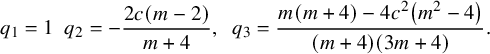
For example, we have: $q_{0} =1, q_1=\frac {6 c m (m+2) }{(m+4) (3 m+4)}$
,
$q_{0} =1, q_1=\frac {6 c m (m+2) }{(m+4) (3 m+4)}$
,
 $$ \begin{align*} q_2=\frac{3 m (3 m+2) \left(4 c^2 (m+2) -2m \right)}{(m+4) (3 m+4) (5 m+4)}, \,\,\, q_3=\frac{12cm (3 m+2)(5 m+2) \left(2 c^2 (m+2) -6m \right)}{(m+4) (3 m+4) (5 m+4) (7 m+4)}.\end{align*} $$
We will show that $\{q_n\}$
is a special case of the associated ultraspherical polynomials.
$\{q_n\}$
is a special case of the associated ultraspherical polynomials.
Let c and $\nu $
be two complex numbers. Let
$\nu $
be two complex numbers. Let $C_n^{(\nu )}(x;c)$
denote the family of associated ultraspherical polynomials with initial conditions
$C_n^{(\nu )}(x;c)$
denote the family of associated ultraspherical polynomials with initial conditions $C_{-1}^{(\nu )}(x;c)=0$
and
$C_{-1}^{(\nu )}(x;c)=0$
and $C_{0}^{(\nu )}(x;c)=1$
(cf. [Reference Bustoz and Ismail5], p. 729). Then they satisfy the following difference equation:
$C_{0}^{(\nu )}(x;c)=1$
(cf. [Reference Bustoz and Ismail5], p. 729). Then they satisfy the following difference equation:
 $$ \begin{align} 2x(n+\nu+c)C_{n}^{(\nu)}(x;c)=(n+c+1)C_{n+1}^{(\nu)}(x;c)+(2\nu+n+c-1)C_{n-1}^{(\nu)}(x;c). \end{align} $$
Choosing $c=\frac {1}{2}+\frac {2}{m}$
and
$c=\frac {1}{2}+\frac {2}{m}$
and $\nu =-\frac {1}{m}$
, this equation becomes the recurrence relation (4.2). Hence, we conclude that polynomials
$\nu =-\frac {1}{m}$
, this equation becomes the recurrence relation (4.2). Hence, we conclude that polynomials $P_{-4,n}$
is a special case of associated ultraspherical polynomials. We immediately have the following:
$P_{-4,n}$
is a special case of associated ultraspherical polynomials. We immediately have the following:
Corollary 4.1. Polynomials $P_{-4,n}$
are non-classical orthogonal polynomials.
$P_{-4,n}$
are non-classical orthogonal polynomials.
5 Orthogonality of $P_{-2,n}$

Polynomials $P_{-2,n}$
satisfy the same recurrence relation as polynomials
$P_{-2,n}$
satisfy the same recurrence relation as polynomials $P_{-4,n}$
but have different initial conditions. Hence, we do not know immediately whether they are associated ultraspherical polynomials and whether they are orthogonal. We will give an independent proof of the orthogonality of these polynomials. Set
$P_{-4,n}$
but have different initial conditions. Hence, we do not know immediately whether they are associated ultraspherical polynomials and whether they are orthogonal. We will give an independent proof of the orthogonality of these polynomials. Set $q_s(c)=P_{-2,2s}(c)$
. In particular, we have
$q_s(c)=P_{-2,2s}(c)$
. In particular, we have
 $$ \begin{align*} q_{1}=1\,\,\, q_{2}=-\frac{2 c (m-2)}{m+4}, \,\,\, q_{3}= \frac{m (m+4)-4 c^2 \left(m^2-4\right)}{(m+4) (3 m+4)}. \end{align*} $$
Now we set $ \overline {q}_n:=q_{n+1}$
,
$ \overline {q}_n:=q_{n+1}$
, $n\geq -1$
. Then polynomials
$n\geq -1$
. Then polynomials $\overline {q}_{n}$
have degree n, and (4.2) becomes
$\overline {q}_{n}$
have degree n, and (4.2) becomes
 $$ \begin{align} 2 (2m n+3m+2)c \overline{q}_{n}=(2 m n+m) \overline{q}_{n-1}+(2m n+5m+4) \overline{q}_{n+1}. \end{align} $$
We recall the following result.
Theorem 5.1 ([Reference Cox, Futorny and Tirao9], Theorem 5.0.4).
Let $\{p_n, n \geq 0\}$
be a sequence of polynomials, where
$\{p_n, n \geq 0\}$
be a sequence of polynomials, where $p_n$
has degree n for any n, satisfying the following recursion
$p_n$
has degree n for any n, satisfying the following recursion
 $$ \begin{align} \chi p_n = a_{n+1}p_{n+1}+b_np_n+c_{n-1}p_{n-1}, && n=0,1,2,\dots \end{align} $$
for some complex numbers $a_{n+1}$
,
$a_{n+1}$
, $b_n$
,
$b_n$
, $c_{n-1}$
,
$c_{n-1}$
, $n=0, 1, 2, \dots $
and
$n=0, 1, 2, \dots $
and $p_{-1}=0$
. Then
$p_{-1}=0$
. Then $\{p_n, n\geq 0\}$
is a sequence of orthogonal polynomials with respect to some (unique) weight measure if and only if
$\{p_n, n\geq 0\}$
is a sequence of orthogonal polynomials with respect to some (unique) weight measure if and only if $b_n\in \mathbb {R}$
and
$b_n\in \mathbb {R}$
and $c_n=\overline {a}_n+1\neq 0$
for all
$c_n=\overline {a}_n+1\neq 0$
for all $n\geq 0.$
We apply the theorem in the case when
 $$ \begin{align*}a_{n+1}=\frac{(2m n+5m+4) }{2 (2m n+3m+2)}, \,\,\, b_{n}=0, \,\,\, c_{n-1}=\frac{(2 m n+m)}{2 (2m n+3m+2)}.\end{align*} $$
Theorem 5.2. The polynomials $P_{-2,n}(c)$
are orthogonal with respect to some weight function.
$P_{-2,n}(c)$
are orthogonal with respect to some weight function.
Proof. It is sufficient to check that there exists a family of orthonormal polynomials $f_n$
and constants
$f_n$
and constants $\lambda _n$
such that
$\lambda _n$
such that $q_n=\lambda _n f_n$
for all n.
$q_n=\lambda _n f_n$
for all n.
We have the following recursion for $f_n$
:
$f_n$
:
 $$ \begin{align*} f_n=\frac{(2 m n+m)\lambda_{n-1}}{2 (2m n+3m+2)c \lambda_{n} } f_{n-1}+\frac{(2m n+5m+4) \lambda_{n+1}}{2 (2m n+3m+2)c \lambda_{n} }f_{n+1}, \end{align*} $$
for $n\geq 1$
.
$n\geq 1$
.
Set
 $$ \begin{align*} A_{n+1} = \frac{(2m n+5m+4) \lambda_{n+1}}{2 (2m n+3m+2) \lambda_{n} }& & C_{n-1}=\frac{(2 m n+m)\lambda_{n-1}}{2 (2m n+3m+2) \lambda_{n} }. \end{align*} $$
Then $A_{n}=C_{n-1}$
if and only if
$A_{n}=C_{n-1}$
if and only if
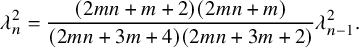 $$ \begin{align*} \lambda_n^2=\frac{(2m n+m+2) (2 m n+m)}{(2m n+3m+4)(2m n+3m+2) }\lambda_{n-1}^2. \end{align*} $$
Taking $\lambda _0 = 1$
, we can find a family of constants
$\lambda _0 = 1$
, we can find a family of constants $\lambda _n$
satisfying this relation.
$\lambda _n$
satisfying this relation.
Appendix
Proof of Theorem 2.1.
The proof generalizes the proof of Theorem 3.1.1 in [Reference Cox, Futorny and Tirao9] in the case $m=2$
. We start off with the generating function
$m=2$
. We start off with the generating function
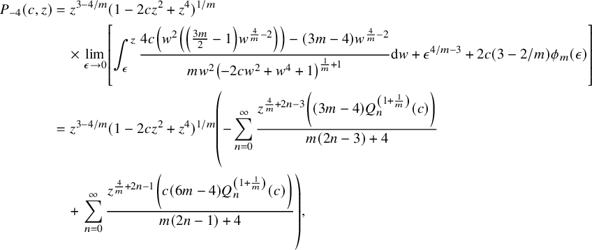 $$ \begin{align*} P_{-4}(c,z)&=z^{3-4/m} (1-2 c z^2+z^4)^{1/m}\\&\quad \times\lim_{\epsilon\to 0}\left[\int_{\epsilon}^{z}\frac{4 c \left(w^2 \left(\left(\frac{3 m}{2}-1\right) w^{\frac{4}{m}-2}\right)\right)-(3 m-4) w^{\frac{4}{m}-2}}{m w^2 \left(-2 c w^2+w^4+1\right)^{\frac{1}{m}+1}} \textrm{d}w+\epsilon^{4/m-3}+2c(3-2/m)\phi_m(\epsilon)\right] \\&=z^{3-4/m} (1-2 c z^2+z^4)^{1/m} \left(-\sum _{n=0}^{\infty } \frac{z^{\frac{4}{m}+2 n-3} \left((3 m-4) Q_n^{\left(1+\frac{1}{m}\right)}(c)\right)}{m (2 n-3)+4}\right.\\& \quad +\left. \sum _{n=0}^{\infty } \frac{z^{\frac{4}{m}+2 n-1} \left(c (6 m-4) Q_n^{\left(1+\frac{1}{m}\right)}(c)\right)}{m (2 n-1)+4}\right), \end{align*} $$
where $Q_n^\lambda (c)$
is the nth-Gegenbauer polynomial. The polynomials
$Q_n^\lambda (c)$
is the nth-Gegenbauer polynomial. The polynomials $Q_n^\lambda (c)$
satisfy the second-order linear differential equation
$Q_n^\lambda (c)$
satisfy the second-order linear differential equation
 $$ \begin{align*} \left(1-c^2\right) y"-c (2 \lambda +1) y'+n y (2 \lambda +n)=0, \end{align*} $$
where the derivatives are with respect to c. Thus, for $\lambda = 1+\frac {1}{m}$
, we get
$\lambda = 1+\frac {1}{m}$
, we get
 $$ \begin{align} \left(1-c^2\right) (Q_n^{\left(1+\frac{1}{m}\right)})"(c)-c \left(\frac{2}{m}+3\right) (Q_n^{\left(1+\frac{1}{m}\right)})'(c)+n \left(\frac{2}{m}+n+2\right) Q_n^{\left(1+\frac{1}{m}\right)}(c)=0. \end{align} $$
Rewriting the expansion formula for $P_{-4}(c,z)$
, we get
$P_{-4}(c,z)$
, we get
 $$ \begin{align} z^{-3+4/m} (1-2 c z^2+z^4)^{-1/m}P_{-4}(c,z)&= \sum _{n=0}^{\infty } \frac{z^{\frac{4}{m}+2 n-1} \left(c (6 m-4) Q_n^{\left(1+\frac{1}{m}\right)}(c)\right)}{m (2 n-1)+4} \nonumber\\& \quad - \sum _{n=0}^{\infty } \frac{z^{\frac{4}{m}+2 n-3} \left((3 m-4) Q_n^{\left(1+\frac{1}{m}\right)}(c)\right)}{m (2 n-3)+4}. \end{align} $$
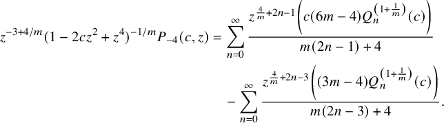
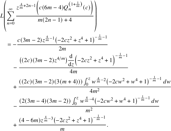
Now we apply the differential operator $L:=(1-c^2)\frac {d^2}{dc^2}-(c(3+\frac {2}{m}))\frac {d}{dc}$
to the right-hand side and use the identity (formula 4.7.27 in [Reference Szegö20])
$L:=(1-c^2)\frac {d^2}{dc^2}-(c(3+\frac {2}{m}))\frac {d}{dc}$
to the right-hand side and use the identity (formula 4.7.27 in [Reference Szegö20])
Then we get
 $$ \begin{align*} L \left(c(-\frac{4}{m}+6) Q_n^{\left(1+\frac{1}{m}\right)}(c)\right)&=\left( (1-c^2)\frac{d^2}{dc^2}-(c(3+2/m))\frac{d}{dc} \right)\left(c(-4/m+6) Q_n^{\left(1+\frac{1}{m}\right)}(c)\right)\\&=-\frac{2 (3 m-2)}{m} \left(2 m (n+1) Q_{n+1}^{\left(1+\frac{1}{m}\right)}(c)\right. \\& \quad +\left. c (n-1) (m n+m+2) Q_n^{\left(1+\frac{1}{m}\right)}(c)\right). \end{align*} $$
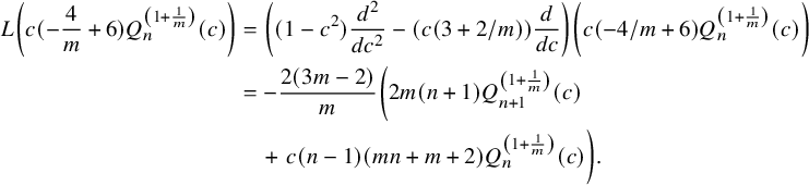
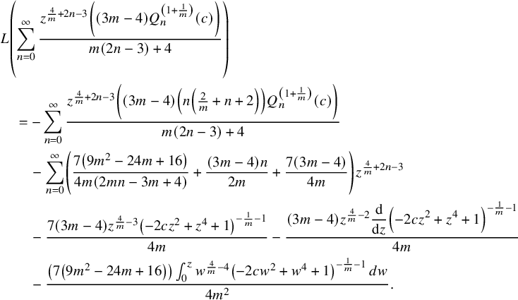
From here, we deduce
 $$ \begin{align*} &L \left(\sum _{n=0}^{\infty } \frac{z^{\frac{4}{m}+2 n-1} \left(c (6 m-4) Q_n^{\left(1+\frac{1}{m}\right)}(c)\right)}{m (2 n-1)+4}\right)\\&\quad =\sum _{n=0}^{\infty } -\frac{z^{\frac{4}{m}+2 n-1} \left((2 (3 m-2)) \left(2 m (n+1) c_{n+1}^{\left(1+\frac{1}{m}\right)}(c)+c (n-1) (m n+m+2) Q_n^{\left(1+\frac{1}{m}\right)}(c)\right)\right)}{m (m (2 n-1)+4)}\\&\quad =\sum _{n=0}^{\infty } -\frac{z^{\frac{4}{m}+2 n-1} \left((2 c (3 m-2) (n-1) (m n+m+2)) Q_n^{\left(1+\frac{1}{m}\right)}(c)\right)}{m (m (2 n-1)+4)}\\&\qquad +\sum _{n=0}^{\infty } -\frac{z^{\frac{4}{m}+2 n-1} \left((4 (3 m-2) (n+1)) c_{n+1}^{\left(1+\frac{1}{m}\right)}(c)\right)}{m (2 n-1)+4}. \end{align*} $$
Since
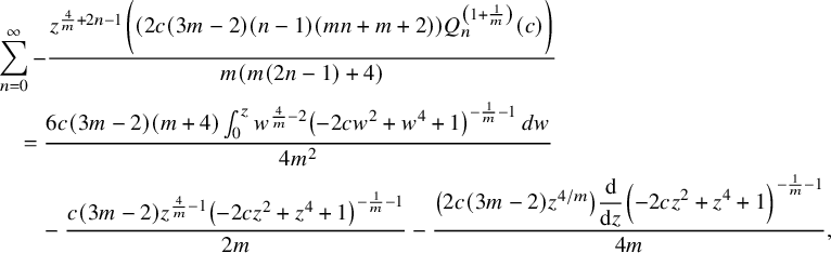
and
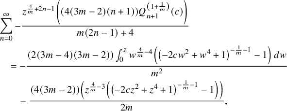 $$ \begin{align*} &\sum _{n=0}^{\infty } -\frac{z^{\frac{4}{m}+2 n-1} \left((4 (3 m-2) (n+1)) Q_{n+1}^{\left(1+\frac{1}{m}\right)}(c)\right)}{m (2 n-1)+4}\\&\quad =-\frac{(2 (3 m-4) (3 m-2)) \int_{0}^z w^{\frac{4}{m}-4} \left(\left(-2 c w^2+w^4+1\right)^{-\frac{1}{m}-1}-1\right) \, dw}{m^2}\\&\qquad -\frac{(4 (3 m-2)) \left(z^{\frac{4}{m}-3} \left(\left(-2 c z^2+z^4+1\right)^{-\frac{1}{m}-1}-1\right)\right)}{2 m}, \end{align*} $$
we get
In addition, we have
Applying the operator L to the left-hand side of (5.4), we get
 $$ \begin{align*} &L \left(z^{\frac{4}{m}-3} \left(-2 c z^2+z^4+1\right)^{-1/m} P_{-4}(c,z)\right)\\&=\frac{z^{\frac{4}{m}-1} \left(-2 c z^2+z^4+1\right)^{-\frac{1}{m}-2} \left(4 c^2 (2 m+1) z^2-2 c (3 m+2) \left(z^4+1\right)+4 (m+1) z^2\right) P_{-4}(c,z)}{m^2}\\&\quad +\frac{z^{\frac{4}{m}-3} \left(-2 c z^2+z^4+1\right)^{-\frac{1}{m}-1} \left(6 c^2 m z^2-c (3 m+2) \left(z^4+1\right)+4 z^2\right) P^{\prime}_{-4}(c,z)}{m}\\&\quad -\left(c^2-1\right) z^{\frac{4}{m}-3} \left(-2 c z^2+z^4+1\right)^{-1/m} P^{\prime\prime}_{n-4}(c,z). \end{align*} $$
Hence, we obtain
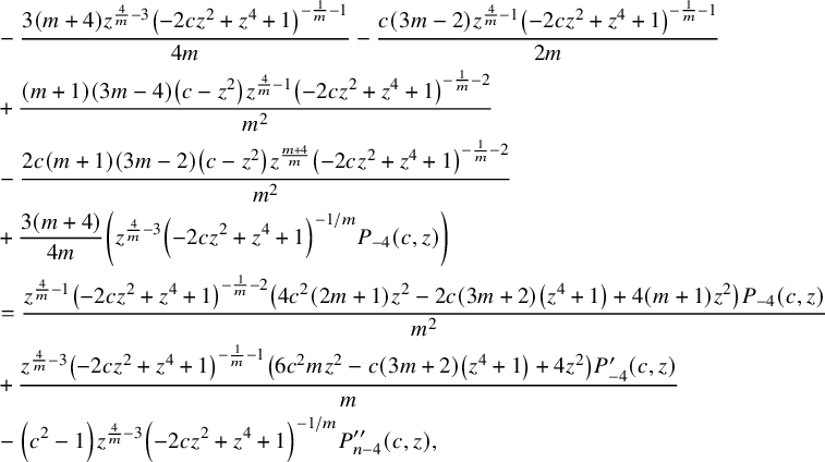 $$ \begin{align*} &-\frac{3 (m+4) z^{\frac{4}{m}-3} \left(-2 c z^2+z^4+1\right)^{-\frac{1}{m}-1}}{4 m}-\frac{c (3 m-2) z^{\frac{4}{m}-1} \left(-2 c z^2+z^4+1\right)^{-\frac{1}{m}-1}}{2 m}\\&+\frac{(m+1) (3 m-4) \left(c-z^2\right) z^{\frac{4}{m}-1} \left(-2 c z^2+z^4+1\right)^{-\frac{1}{m}-2}}{m^2}\\&-\frac{2 c (m+1) (3 m-2) \left(c-z^2\right) z^{\frac{m+4}{m}} \left(-2 c z^2+z^4+1\right)^{-\frac{1}{m}-2}}{m^2}\\&+\frac{3 (m+4)}{4 m}\left(z^{\frac{4}{m}-3}\left(-2 c z^2+z^4+1\right)^{-1/m}P_{-4}(c,z)\right)\\&=\frac{z^{\frac{4}{m}-1} \left(-2 c z^2+z^4+1\right)^{-\frac{1}{m}-2} \left(4 c^2 (2 m+1) z^2-2 c (3 m+2) \left(z^4+1\right)+4 (m+1) z^2\right) P_{-4}(c,z)}{m^2}\\&+\frac{z^{\frac{4}{m}-3} \left(-2 c z^2+z^4+1\right)^{-\frac{1}{m}-1} \left(6 c^2 m z^2-c (3 m+2) \left(z^4+1\right)+4 z^2\right) P^{\prime}_{-4}(c,z)}{m}\\&-\left(c^2-1\right) z^{\frac{4}{m}-3} \left(-2 c z^2+z^4+1\right)^{-1/m} P^{\prime\prime}_{n-4}(c,z), \end{align*} $$
which gives us
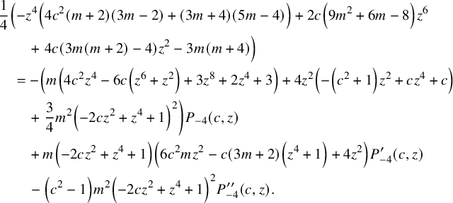 $$ \begin{align*} &\frac{1}{4} \left(-z^4 \left(4 c^2 (m+2) (3 m-2)+(3 m+4) (5 m-4)\right)+2 c \left(9 m^2+6 m-8\right) z^6\right. \\& \qquad + \left. 4 c (3 m (m+2)-4) z^2-3 m (m+4)\right)\\& \quad =-\left(m \left(4 c^2 z^4-6 c \left(z^6+z^2\right)+3 z^8+2 z^4+3\right)+4 z^2 \left(-\left(c^2+1\right) z^2+c z^4+c\right)\right.\\& \qquad + \left. \frac{3}{4} m^2 \left(-2 c z^2+z^4+1\right)^2\right) P_{-4}(c,z)\\& \qquad +m \left(-2 c z^2+z^4+1\right) \left(6 c^2 m z^2-c (3 m+2) \left(z^4+1\right)+4 z^2\right) P^{\prime}_{-4}(c,z)\\& \qquad -\left(c^2-1\right) m^2 \left(-2 c z^2+z^4+1\right)^2 P^{\prime\prime}_{-4}(c,z). \end{align*} $$
Expanding this out and writing $P_{-4,k}(c)$
as
$P_{-4,k}(c)$
as $P_k$
, we will have the following equality:
$P_k$
, we will have the following equality:
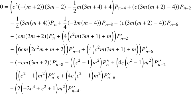 $$ \begin{align} 0&=\left(c^2 (-(m+2)) (3 m-2)-\frac{1}{2} m (3 m+4)+4\right) P_{n-4} +(c (3 m (m+2)-4)) P_{n-2} \nonumber\\&\quad -\frac{1}{4} (3 m (m+4)) P_n +\frac{1}{4} (-3 m (m+4)) P_{n-8} +(c (3 m (m+2)-4)) P_{n-6} \nonumber\\&\quad -(c m (3 m+2)) P^{\prime}_n +\left(4 \left(c^2 m (3 m+1)+m\right)\right) P^{\prime}_{n-2} \nonumber\\&\quad -\left(6 c m \left(2 c^2 m+m+2\right)\right) P^{\prime}_{n-4} +\left(4 \left(c^2 m (3 m+1)+m\right)\right) P^{\prime}_{n-6} \nonumber\\&\quad +(-c m (3 m+2)) P^{\prime}_{n-8} -\left(\left(c^2-1\right) m^2\right) P^{\prime\prime}_n +\left(4 c \left(c^2-1\right) m^2\right) P^{\prime\prime}_{n-2} \nonumber\\&\quad -\left(\left(c^2-1\right) m^2\right) P^{\prime\prime}_{n-8} +\left(4 c \left(c^2-1\right) m^2\right) P^{\prime\prime}_{n-6} \nonumber\\&\quad +\left(2 \left(-2 c^4+c^2+1\right) m^2\right) P^{\prime\prime}_{n-4}. \end{align} $$
We now differentiate twice with respect to c the recursion 2.1:
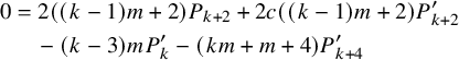 $$ \begin{align} 0&=2 ((k-1) m+2) P_{k+2} +2 c ((k-1) m+2) P^{\prime}_{k+2} \nonumber\\& \quad -(k-3) m P^{\prime}_k -(k m+m+4) P^{\prime}_{k+4} \end{align} $$
 $$ \begin{align} 0&=(4 (k-1) m+8) P^{\prime}_{k+2} +2 c ((k-1) m+2) P^{\prime\prime}_{k+2} \nonumber\\&\quad -(k m+m+4) P^{\prime\prime}_{k+4} -(k-3) m P^{\prime\prime}_k. \end{align} $$
Substituting $k=n-8$
in the last equation, we obtain
$k=n-8$
in the last equation, we obtain
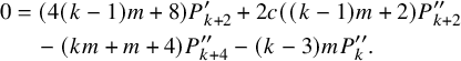
 $$ \begin{align} 0&=4 (m (n-9)+2) P^{\prime}_{n-6} -m (n-11) P^{\prime\prime}_{n-8} \nonumber\\& \quad +2 c (m (n-9)+2) P^{\prime\prime}_{n-6} -(m (n-7)+4) P^{\prime\prime}_{n-4}. \end{align} $$
Multiplying (5.6) by $-11+n$
and adding it to the above equation multiplied by
$-11+n$
and adding it to the above equation multiplied by $(1-c^2) m$
gives us
$(1-c^2) m$
gives us
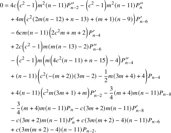 $$ \begin{align} 0&=4 c \left(c^2-1\right) m^2 (n-11) P^{\prime\prime}_{n-2} -\left(c^2-1\right) m^2 (n-11) P^{\prime\prime}_n \nonumber\\&\quad +4 m \left(c^2 (2 m (n-12)+n-13)+(m+1) (n-9)\right) P^{\prime}_{n-6} \nonumber\\&\quad -6 c m (n-11) \left(2 c^2 m+m+2\right) P^{\prime}_{n-4} \nonumber\\&\quad +2 c \left(c^2-1\right) m (m (n-13)-2) P^{\prime\prime}_{n-6} \nonumber\\&\quad -\left(c^2-1\right) m \left(m \left(4 c^2 (n-11)+n-15\right)-4\right) P^{\prime\prime}_{n-4} \nonumber\\&\quad +(n-11) \left(c^2 (-(m+2)) (3 m-2)-\frac{1}{2} m (3 m+4)+4\right) P_{n-4} \nonumber\\&\quad +4 (n-11) \left(c^2 m (3 m+1)+m\right) P^{\prime}_{n-2} -\frac{3}{4} (m+4) m (n-11) P_{n-8} \nonumber\\&\quad -\frac{3}{4} (m+4) m (n-11) P_n -c (3 m+2) m (n-11) P^{\prime}_{n-8} \nonumber\\&\quad -c (3 m+2) m (n-11) P^{\prime}_n +c (3 m (m+2)-4) (n-11) P_{n-6} \nonumber\\&\quad +c (3 m (m+2)-4) (n-11) P_{n-2}. \end{align} $$
Now substitute $k=n-8$
in (5.7) to get
$k=n-8$
in (5.7) to get
 $$ \begin{align} 0&=2 (m (n-9)+2) P_{n-6} -m (n-11) P^{\prime}_{n-8} +2 c (m (n-9)+2) P^{\prime}_{n-6} \nonumber\\&\quad -(m (n-7)+4) P^{\prime}_{n-4}. \end{align} $$
Multiplying this equation by $-c (2+3 m)$
and adding it to the previous equation, we obtain
$-c (2+3 m)$
and adding it to the previous equation, we obtain
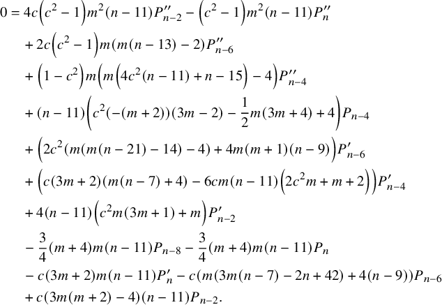 $$ \begin{align*} 0&=4 c \left(c^2-1\right) m^2 (n-11) P^{\prime\prime}_{n-2} -\left(c^2-1\right) m^2 (n-11) P^{\prime\prime}_n \\&\quad +2 c \left(c^2-1\right) m (m (n-13)-2) P^{\prime\prime}_{n-6} \\&\quad +\left(1-c^2\right) m \left(m \left(4 c^2 (n-11)+n-15\right)-4\right) P^{\prime\prime}_{n-4} \\&\quad +(n-11) \left(c^2 (-(m+2)) (3 m-2)-\frac{1}{2} m (3 m+4)+4\right) P_{n-4} \\&\quad +\left(2 c^2 (m (m (n-21)-14)-4)+4 m (m+1) (n-9)\right) P^{\prime}_{n-6} \\&\quad +\left(c (3 m+2) (m (n-7)+4)-6 c m (n-11) \left(2 c^2 m+m+2\right)\right) P^{\prime}_{n-4} \\&\quad +4 (n-11) \left(c^2 m (3 m+1)+m\right) P^{\prime}_{n-2} \\&\quad -\frac{3}{4} (m+4) m (n-11) P_{n-8} -\frac{3}{4} (m+4) m (n-11) P_n \\&\quad -c (3 m+2) m (n-11) P^{\prime}_n -c (m (3 m (n-7)-2 n+42)+4 (n-9)) P_{n-6} \\&\quad +c (3 m (m+2)-4) (n-11) P_{n-2}. \end{align*} $$
Finally, substitute $k=n-8$
in (2.1), multiply it by
$k=n-8$
in (2.1), multiply it by $-3 (4+m)$
and add to the previous equation multiplied by
$-3 (4+m)$
and add to the previous equation multiplied by $4$
:
$4$
:
 $$ \begin{align*} 0&=-2 c (m (m (9 n-69)+8 n-18)+8 (n-6)) P_{n-6} \\&\quad +\left(-4 c^2 (m+2) (3 m-2) (n-11)+16 (m+n-8)+m (4 n-3 m (n-15))\right) P_{n-4} \\&\quad +4 c (3 m (m+2)-4) (n-11) P_{n-2} -3 m (m+4) (n-11) P_n \\&\quad +\left(8 c^2 (m (m (n-21)-14)-4)+16 m (m+1) (n-9)\right) P^{\prime}_{n-6} \\&\quad +4 \left(c (3 m+2) (m (n-7)+4)-6 c m (n-11) \left(2 c^2 m+m+2\right)\right) P^{\prime}_{n-4} \\&\quad +16 (n-11) \left(c^2 m (3 m+1)+m\right) P^{\prime}_{n-2} -4 c m (3 m+2) (n-11) P^{\prime}_n \\&\quad +8 c \left(c^2-1\right) m (m (n-13)-2) P^{\prime\prime}_{n-6} \\&\quad +4 \left(1-c^2\right) m \left(m \left(4 c^2 (n-11)+n-15\right)-4\right) P^{\prime\prime}_{n-4} \\&\quad +16 c \left(c^2-1\right) m^2 (n-11) P^{\prime\prime}_{n-2} -4 \left(c^2-1\right) m^2 (n-11) P^{\prime\prime}_n. \end{align*} $$
We obtained the equation without terms with index $n-8$
.
$n-8$
.
The next step is to eliminate $P_{n-6}$
. After setting
$P_{n-6}$
. After setting $k=n-6$
in (5.8), (5.7) and in the recursion, we obtain the following equations:
$k=n-6$
in (5.8), (5.7) and in the recursion, we obtain the following equations:
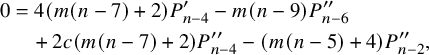 $$ \begin{align} 0&=4 (m (n-7)+2) P^{\prime}_{n-4} -m (n-9) P^{\prime\prime}_{n-6} \nonumber\\&\quad +2 c (m (n-7)+2) P^{\prime\prime}_{n-4} -(m (n-5)+4) P^{\prime\prime}_{n-2}, \end{align} $$
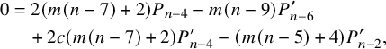 $$ \begin{align} 0&=2 (m (n-7)+2) P_{n-4} -m (n-9) P^{\prime}_{n-6} \nonumber\\&\quad +2 c (m (n-7)+2) P^{\prime}_{n-4} -(m (n-5)+4) P^{\prime}_{n-2}, \end{align} $$
 $$ \begin{align*} \kern65pt 0=-m (n-9) P_{n-6} +2 c (m (n-7)+2) P_{n-4} -(m (n-5)+4) P_{n-2}. \end{align*} $$
Proceeding as in the previous case and using these three equations, we can eliminate all terms with index $n-6$
:
$n-6$
:
 $$ \begin{align*} 0&=\left(-64 c^3 (m+1) (2 m+1) (m (n-4)+2)-4 c m (m (m (n (3 n-104)+629)\right.\\&\quad + 2 (n-54) n+714)-24 n+184)\Big) P^{\prime}_{n-4} \\&\quad -4 \left(c^2-1\right) m^3 (n-11) (n-9) P^{\prime\prime}_n \\&\quad +\left(m (n-9) \left(m^2 (29 n-179)+36 m (n-4)+16 (n-4)\right)\right.\\&\quad -\left. 16 c^2 (m+1) (2 m+1) (n-4) (m (n-6)+4)\right) P_{n-4} \\&\quad +m \left((m (n-5)+4) \left(8 c^2 \left(-m (n-21)+\frac{4}{m}+14\right)-16 (m+1) (n-9)\right)\right.\\&\quad+ 16 (n-11) (n-9) \left(c^2 m (3 m+1)+m\right)\bigg) P^{\prime}_{n-2} \\&\quad -4 \left(c^2-1\right) m \left(16 c^2 (m+1) (2 m+1)+m (n-9) (m (n-15)-4)\right) P^{\prime\prime}_{n-4} \\&\quad +8 c \left(c^2-1\right) m (m (m ((n-22) n+133)-2 n+42)+8) P^{\prime\prime}_{n-2} \\&\quad -3 (m+4) m^2 (n-11) (n-9) P_n -4 c (3 m+2) m^2 (n-11) (n-9) P^{\prime}_n \\&\quad +(4 c m (3 m (m+2)-4) (n-11) (n-9)\\&\quad +2 c (m (n-5)+4) (m (m (9 n-69)+8 n-18)+8 (n-6))) P_{n-2}. \end{align*} $$
The next step is to eliminate terms with index $n-4$
. Substituting
$n-4$
. Substituting $k=n-6$
in (5.8), (5.7) and in the recursion, we obtain the following equations:
$k=n-6$
in (5.8), (5.7) and in the recursion, we obtain the following equations:
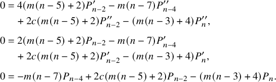 $$ \begin{align*} 0&=4 (m (n-5)+2) P^{\prime}_{n-2} -m (n-7) P^{\prime\prime}_{n-4} \\&\quad +2 c (m (n-5)+2) P^{\prime\prime}_{n-2} -(m (n-3)+4) P^{\prime\prime}_n,\\[4pt]0&=2 (m (n-5)+2) P_{n-2} -m (n-7) P^{\prime}_{n-4} \\&\quad +2 c (m (n-5)+2) P^{\prime}_{n-2} -(m (n-3)+4) P^{\prime}_n,\\[4pt]0&=-m (n-7) P_{n-4} +2 c (m (n-5)+2) P_{n-2} -(m (n-3)+4) P_n. \end{align*} $$
Using these equations, we can eliminate terms with index $n-4$
:
$n-4$
:
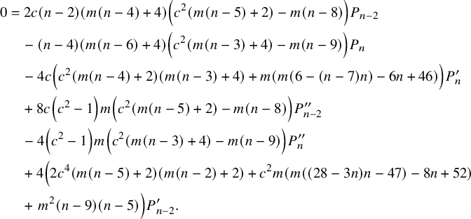 $$ \begin{align} 0&=2 c (n-2) (m (n-4)+4) \left(c^2 (m (n-5)+2)-m (n-8)\right) P_{n-2} \nonumber\\&\quad -(n-4) (m (n-6)+4) \left(c^2 (m (n-3)+4)-m (n-9)\right) P_n \nonumber\\&\quad -4 c \left(c^2 (m (n-4)+2) (m (n-3)+4)+m (m (6-(n-7) n)-6 n+46)\right) P^{\prime}_n \nonumber\\&\quad +8 c \left(c^2-1\right) m \left(c^2 (m (n-5)+2)-m (n-8)\right) P^{\prime\prime}_{n-2} \nonumber\\&\quad -4 \left(c^2-1\right) m \left(c^2 (m (n-3)+4)-m (n-9)\right) P^{\prime\prime}_n \nonumber\\&\quad +4 \left(2 c^4 (m (n-5)+2) (m (n-2)+2)+c^2 m (m ((28-3 n) n-47)-8 n+52)\right.\nonumber\\&\quad +\left. m^2 (n-9) (n-5)\right) P^{\prime}_{n-2}. \end{align} $$
Finally, we will eliminate all terms with index $n-2$
. Substituting
$n-2$
. Substituting $k=n-2$
in (5.8), (5.7) and in the recursion, we obtain
$k=n-2$
in (5.8), (5.7) and in the recursion, we obtain
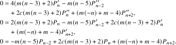 $$ \begin{align*} 0&=4 (m (n-3)+2) P^{\prime}_n -m (n-5) P^{\prime\prime}_{n-2} \\& \quad +2 c (m (n-3)+2) P^{\prime\prime}_n +(m (-n)+m-4) P^{\prime\prime}_{n+2}, \\0&=2 (m (n-3)+2) P_n -m (n-5) P^{\prime}_{n-2} +2 c (m (n-3)+2) P^{\prime}_n \\& \quad +(m (-n)+m-4) P^{\prime}_{n+2}, \\0&=-m (n-5) P_{n-2} +2 c (m (n-3)+2) P_n +(m (-n)+m-4) P_{n+2}. \end{align*} $$
These equations substitution $n\rightarrow n-2$
lead to the following equation:
$n\rightarrow n-2$
lead to the following equation:
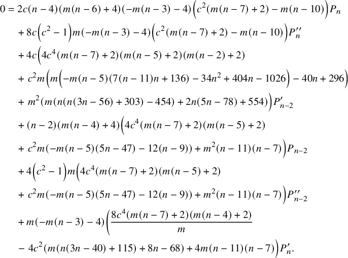 $$ \begin{align} 0&=2 c (n-4) (m (n-6)+4) (-m (n-3)-4) \left(c^2 (m (n-7)+2)-m (n-10)\right) P_n \nonumber \\&\quad +8 c \left(c^2-1\right) m (-m (n-3)-4) \left(c^2 (m (n-7)+2)-m (n-10)\right) P^{\prime\prime}_n \nonumber \\&\quad +4 c \left(4 c^4 (m (n-7)+2) (m (n-5)+2) (m (n-2)+2)\right.\nonumber\\&\quad +\left.c^2 m \left(m \left(-m (n-5) (7 (n-11) n+136)-34 n^2+404 n-1026\right)-40 n+296\right)\right.\nonumber\\&\quad +\left.m^2 (m (n (n (3 n-56)+303)-454)+2 n (5 n-78)+554)\right) P^{\prime}_{n-2} \nonumber \\&\quad +(n-2) (m (n-4)+4) \left(4 c^4 (m (n-7)+2) (m (n-5)+2)\right.\nonumber\\&\quad +\left.c^2 m (-m (n-5) (5 n-47)-12 (n-9))+m^2 (n-11) (n-7)\right) P_{n-2} \nonumber \\&\quad +4 \left(c^2-1\right) m \left(4 c^4 (m (n-7)+2) (m (n-5)+2)\right.\nonumber\\&\quad +\left.c^2 m (-m (n-5) (5 n-47)-12 (n-9))+m^2 (n-11) (n-7)\right) P^{\prime\prime}_{n-2} \nonumber \\&\quad +m (-m (n-3)-4) \left(\frac{8 c^4 (m (n-7)+2) (m (n-4)+2)}{m}\right.\nonumber\\&\quad -\left.4 c^2 (m (n (3 n-40)+115)+8 n-68)+4 m (n-11) (n-7)\right) P^{\prime}_n. \end{align} $$
Combining this with (5.14), we obtain
 $$ \begin{align} 0&=2 c (n-2) (m (n-4)+4) \left(c^2 (m (n-5)+2)-m (n-8)\right) P_{n-2} \nonumber\\&\quad -(n-4) (m (n-6)+4) \left(c^2 (m (n-3)+4)-m (n-9)\right) P_n \nonumber\\&\quad -4 c \left(c^2 (m (n-4)+2) (m (n-3)+4)+m (m (6-(n-7) n)-6 n+46)\right) P^{\prime}_n \nonumber\\&\quad +8 c \left(c^2-1\right) m \left(c^2 (m (n-5)+2)-m (n-8)\right) P^{\prime\prime}_{n-2} \nonumber\\&\quad -4 \left(c^2-1\right) m \left(c^2 (m (n-3)+4)-m (n-9)\right) P^{\prime\prime}_n \nonumber\\&\quad +4 \left(2 c^4 (m (n-5)+2) (m (n-2)+2)+c^2 m (m ((28-3 n) n-47)-8 n+52)\right.\nonumber\\&\quad +\left. m^2 (n-9) (n-5)\right) P^{\prime}_{n-2}. \end{align} $$
Now we use (5.16) and (5.15) to simplify the coefficient by $P^{\prime \prime }_{n-2}$
. Combining them, multiplying (5.16) by
$P^{\prime \prime }_{n-2}$
. Combining them, multiplying (5.16) by $-2 c (mn-7m+2)$
and adding it to (5.15) gives
$-2 c (mn-7m+2)$
and adding it to (5.15) gives
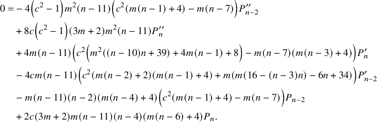 $$ \begin{align*} 0=&-4 \left(c^2-1\right) m^2 (n-11) \left(c^2 (m (n-1)+4)-m (n-7)\right) P^{\prime\prime}_{n-2} \\&+8 c \left(c^2-1\right) (3 m+2) m^2 (n-11) P^{\prime\prime}_n \\&+4 m (n-11) \left(c^2 \left(m^2 ((n-10) n+39)+4 m (n-1)+8\right)-m (n-7) (m (n-3)+4)\right) P^{\prime}_n \\&-4 c m (n-11) \left(c^2 (m (n-2)+2) (m (n-1)+4)+m (m (16-(n-3) n)-6 n+34)\right) P^{\prime}_{n-2} \\&-m (n-11) (n-2) (m (n-4)+4) \left(c^2 (m (n-1)+4)-m (n-7)\right) P_{n-2} \\&+2 c (3 m+2) m (n-11) (n-4) (m (n-6)+4) P_n. \end{align*} $$
From now on, we assume that $n> 11$
. Then the equation simplifies to
$n> 11$
. Then the equation simplifies to
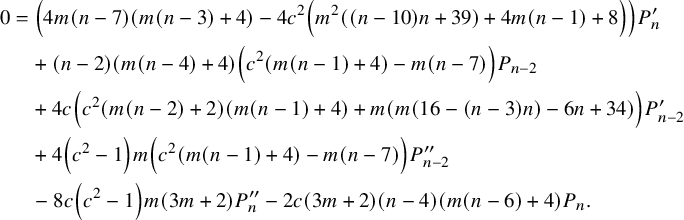 $$ \begin{align} 0&=\left(4 m (n-7) (m (n-3)+4)-4 c^2 \left(m^2 ((n-10) n+39)+4 m (n-1)+8\right)\right) P^{\prime}_n \nonumber\\&\quad +(n-2) (m (n-4)+4) \left(c^2 (m (n-1)+4)-m (n-7)\right) P_{n-2} \nonumber\\&\quad +4 c \left(c^2 (m (n-2)+2) (m (n-1)+4)+m (m (16-(n-3) n)-6 n+34)\right) P^{\prime}_{n-2} \nonumber\\&\quad +4 \left(c^2-1\right) m \left(c^2 (m (n-1)+4)-m (n-7)\right) P^{\prime\prime}_{n-2} \nonumber\\&\quad -8 c \left(c^2-1\right) m (3 m+2) P^{\prime\prime}_n -2 c (3 m+2) (n-4) (m (n-6)+4) P_n. \end{align} $$
Multiplying it by $-2 c (m n-5m+2)$
and adding it to (5.14) multiplied by
$-2 c (m n-5m+2)$
and adding it to (5.14) multiplied by $4+mn-m $
, we get
$4+mn-m $
, we get
 $$ \begin{align} 0&=\left(4 c^2 \left(m^2 ((n-6) n+23)+4 m (n+1)+8\right)-4 m (n-5) (m (n-1)+4)\right) P^{\prime}_{n-2} \nonumber\\&\quad +(n-4) (m (n-6)+4) \left(c^2 m (n-7)-m n+m-4\right) P_n \nonumber\\&\quad -4 c \left(m \left(c^2 (n-7) (m (n-6)+2)-m ((n-13) n+24)-2 n+38\right)+8\right) P^{\prime}_n \nonumber\\&\quad +8 c \left(c^2-1\right) m (3 m+2) P^{\prime\prime}_{n-2} \nonumber\\&\quad +4 \left(c^2-1\right) m \left(c^2 m (n-7)-m n+m-4\right) P^{\prime\prime}_n \nonumber\\&\quad +2 c (3 m+2) (n-2) (m (n-4)+4) P_{n-2}. \end{align} $$
Multiplying this equation by $c (-m n+m-4)$
and adding it to (5.17) multiplied by
$c (-m n+m-4)$
and adding it to (5.17) multiplied by $6 m+4$
, we get
$6 m+4$
, we get
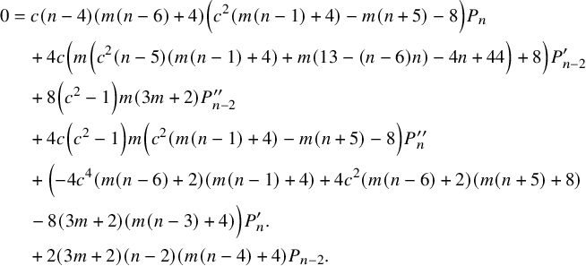 $$ \begin{align} 0&=c (n-4) (m (n-6)+4) \left(c^2 (m (n-1)+4)-m (n+5)-8\right) P_n \nonumber\\&\quad +4 c \left(m \left(c^2 (n-5) (m (n-1)+4)+m (13-(n-6) n)-4 n+44\right)+8\right) P^{\prime}_{n-2} \nonumber\\&\quad +8 \left(c^2-1\right) m (3 m+2) P^{\prime\prime}_{n-2} \nonumber\\&\quad +4 c \left(c^2-1\right) m \left(c^2 (m (n-1)+4)-m (n+5)-8\right) P^{\prime\prime}_n \nonumber\\&\quad +\left(-4 c^4 (m (n-6)+2) (m (n-1)+4)+4 c^2 (m (n-6)+2) (m (n+5)+8)\right.\nonumber\\&\quad - 8 (3 m+2) (m (n-3)+4)\Big) P^{\prime}_n .\nonumber\\&\quad +2 (3 m+2) (n-2) (m (n-4)+4) P_{n-2}. \end{align} $$
Multiplying it by $-c$
and adding to (5.18), we obtain the following equation:
$-c$
and adding to (5.18), we obtain the following equation:
 $$ \begin{align} 0&=4 \left(c^2-1\right) m P^{\prime\prime}_n +(n-4) (m (n-6)+4) P_n \nonumber \\&\quad +4 m (n-5) P^{\prime}_{n-2} -4 c (m (n-6)+2) P^{\prime}_n. \end{align} $$
Differentiate the last equation with respect to c to get
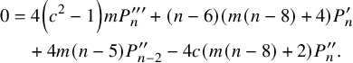 $$ \begin{align} 0&=4 \left(c^2-1\right) m P^{\prime\prime\prime}_n +(n-6) (m (n-8)+4) P^{\prime}_n \nonumber \\&\quad +4 m (n-5) P^{\prime\prime}_{n-2} -4 c (m (n-8)+2) P^{\prime\prime}_n. \end{align} $$
Multiplying it by $-2 \left (c^2-1\right ) (3 m+2)$
and adding to (5.19) multiplied by
$-2 \left (c^2-1\right ) (3 m+2)$
and adding to (5.19) multiplied by $n-5$
gives us the following equation:
$n-5$
gives us the following equation:
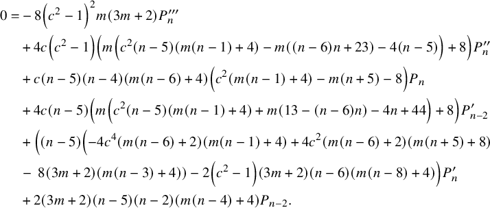 $$ \begin{align*} 0=&-8 \left(c^2-1\right)^2 m (3 m+2) P^{\prime\prime\prime}_n \\&+4 c \left(c^2-1\right) \left(m \left(c^2 (n-5) (m (n-1)+4)-m ((n-6) n+23)-4 (n-5)\right)+8\right) P^{\prime\prime}_n \\&+c (n-5) (n-4) (m (n-6)+4) \left(c^2 (m (n-1)+4)-m (n+5)-8\right) P_n \\&+4 c (n-5) \left(m \left(c^2 (n-5) (m (n-1)+4)+m (13-(n-6) n)-4 n+44\right)+8\right) P^{\prime}_{n-2} \\&+\left((n-5) \left(-4 c^4 (m (n-6)+2) (m (n-1)+4)+4 c^2 (m (n-6)+2) (m (n+5)+8)\right.\right.\\& -\left.\left. 8 (3 m+2) (m (n-3)+4)\right)-2 \left(c^2-1\right) (3 m+2) (n-6) (m (n-8)+4)\right) P^{\prime}_n \\&+2 (3 m+2) (n-5) (n-2) (m (n-4)+4) P_{n-2}. \end{align*} $$
Multiplying now (5.20) by $c \left (m \left (c^2 (n-5) (m (n-1)+4)+m (13-(n-6) n)-4 n+44\right )+8\right )$
and adding it to the equation above multiplied by
$c \left (m \left (c^2 (n-5) (m (n-1)+4)+m (13-(n-6) n)-4 n+44\right )+8\right )$
and adding it to the equation above multiplied by $-m$
gives the following equation:
$-m$
gives the following equation:
 $$ \begin{align*} 0&=-24 c \left(c^2-1\right) m^2 P^{\prime\prime}_n -4 \left(c^2-1\right)^2 m^2 P^{\prime\prime\prime}_n \\&\quad +\left(c^2 (m (3 n (m (n-6)+4)-40)+16)\right.\\& \quad + m (-3 m ((n-6) n+4)-12 n+56)\Big) P^{\prime}_n \\&\quad +m (n-5) (n-2) (m (n-4)+4) P_{n-2} \\&\quad -c (n-4) (m (n-6)+4) (m (n-2)+2) P_n. \end{align*} $$
If we differentiate this equation, multiply by $-4$
and add to (5.20) multiplied by
$-4$
and add to (5.20) multiplied by $(n-2) (m n-4m+4)$
, we will come to the desired linear differential equation of order
$(n-2) (m n-4m+4)$
, we will come to the desired linear differential equation of order $4$
. This proves the theorem.
$4$
. This proves the theorem.
Competing interest
The authors have no competing interests to declare.
Funding statement
Felipe Albino dos Santos aknowledges the support from Universidade Presbiteriana Mackenzie. Vyacheslav Futorny was supported by China NSF grant (No.12350710178). Mikhail Neklyudov, who is a member of the CNPq-Brazil (grant 443594/2023-6) and CAPES MATH AMSUD grant teams, acknowledges the collaborative support of these projects. He also acknowledges support from Universidade Federal do Amazonas and Coordenação de Aperfeiçoamento de Pessoal de Nível Superior (CAPES).
Data availability statement
All the data are available in the manuscript.
Ethical standards
The research meets all ethical guidelines, including adherence to the legal requirements of the study country.
Author contributions
F.A.S., M.N. and V.F. designed the study, wrote the first draft, revised the manuscript and approved the final version of the manuscript.


 Open access