

1. Introduction
In diploid species the genotype of each individual consists of two copies of each (autosomal) chromosome, one inherited from each parent. The genetic material originating from the same parental source is called a haplotype. The haplotype information is essential in numerous genetic studies, e.g. in linkage analysis of pedigree data as well as in association analysis of population-based data. Unfortunately, haplotypes can usually be only partially observed from the unphased genotype data, because common laboratory techniques can identify only the two copies of alleles at each locus, but cannot specify which multilocus combinations of alleles reside on the same chromosome, i.e. which alleles belong to the same haplotype. The corresponding missing data problem – to resolve the genotype data of each individual into two haplotypes – is known as the haplotyping problem.
In the future, practical molecular technologies providing haplotype information may be available to a large community of researchers, but currently this seems not yet to be the case. Experimental procedures are often costly (Douglas et al., Reference Douglas, Boehnke, Gillanders, Trent and Gruber2001), or may have limitations on the number of loci and/or number of samples that can be analysed in practice (Zhang et al., Reference Zhang, Zhu, Shendure, Porreca, Aach, Mitra and Church2006a). Deduction and inheritance rules between subsequent generations can reduce ambiguity substantially for multiallelic (informative) markers in pedigree-based haplotyping algorithms (see Wijsman, Reference Wijsman1987). However, statistical estimation of haplotype patterns from pedigree data (e.g. Sobel & Lange, Reference Sobel and Lange1996; Abecasis et al., Reference Abecasis, Cherny, Cookson and Cardon2002; Qian & Beckmann, Reference Qian and Beckmann2002; Fishelson et al., Reference Fishelson, Dovgolevsky and Geiger2005; Albers et al., Reference Albers, Heskes and Kappen2007) as well as from population-based data (e.g. Clark, Reference Clark1990; Long et al., Reference Long, Williams and Urbanek1995; Niu et al., Reference Niu, Qin, Xu and Liu2002; Stephens & Scheet, Reference Stephens and Scheet2005; Gasbarra & Sillanpää, Reference Gasbarra and Sillanpää2006; Zhang et al., Reference Zhang, Niu and Liu2006b) is usually required before subsequent genetic analyses can be conducted. In some cases, however, the unobserved haplotypes are handled as nuisance parameters in the main linkage or association analysis (e.g. Uimari & Sillanpää, Reference Uimari and Sillanpää2001). Because of the extensive application of the haplotype information in genetic studies, possible reductions of haplotyping costs are of great importance. The International HapMap Project (International HapMap Consortium, 2003, 2005, 2007) aims at indexing the detailed haplotype variation in several human populations. One possible application of the HapMap data is in identifying tag single nucleotide polymorphisms (SNPs), polymorphic positions on the human genome that carry a considerable amount of information on their neighbouring sites. By typing only such tag SNPs, instead of all available SNPs in the region of interest, the number of genotypings and thus the overall cost of association studies could be reduced.
In this article, we consider DNA pooling as a complementary way to reduce the number of genotypings. The idea is to pool equal amounts of DNA from several individuals and to analyse the allele constitution of the whole pool in one genotyping. The achieved quantitative information about the alleles has been found to be quite precise (Norton et al., Reference Norton, Williams, Williams, Spurlock, Kirov, Morris, Hoogendoorn, Owen and O'Donovan2002; Sham et al., Reference Sham, Bader, Craig, O'Donovan and Owen2002), and thus pooling techniques can substantially reduce the cost of studies that involve only single locus allele frequencies of populations. DNA pooling has been suggested as a strategy for whole genome association studies (Sham et al., Reference Sham, Bader, Craig, O'Donovan and Owen2002; Butcher et al., Reference Butcher, Meaburn, Liu, Fernandez, Hill, Al-Chalabi, Plomin, Schalkwyk and Craig2004; Tamiya et al., Reference Tamiya, Shinya, Imanishi, Ikuta, Makino, Okamoto, Furugaki, Matsumoto, Mano, Ando, Nozaki, Yukawa, Nakashige, Yamaguchi, Ishibashi, Yonekura, Nakami, Takayama, Endo, Saruwatari, Yagura, Yoshikawa, Fujimoto, Oka, Chiku, Linsen, Giphart, Kulski, Fukazawa, Hashimoto, Kimura, Hoshina, Suzuki, Hotta, Mochida, Minezaki, Komai, Shiozawa, Taniguchi, Yamanaka, Kamatani, Gojobori, Bahram and Inoko2005; Yang et al., Reference Yang, Pan, Lin and Fann2006), genetic map construction (Gasbarra & Sillanpää, Reference Gasbarra and Sillanpää2006), family-based association testing (Risch & Teng, Reference Risch and Teng1998; Lee, Reference Lee2005; Zou & Zhao, Reference Zou and Zhao2005), estimation of linkage disequilibrium (Pfeiffer et al., Reference Pfeiffer, Rutter, Gail, Struewing and Gastwirth2002; Ito et al., Reference Ito, Chiku, Inoue, Tomita, Morisaki, Morisaki and Kamatani2003), linkage disequilibrium mapping (Johnson, Reference Johnson2005, Reference Johnson2007) and quantitative trait locus mapping based on family data (Wang et al., Reference Wang, Koehler and Dekkers2007). The dimension of the corresponding haplotyping problem increases as material from several individuals is pooled together. Unlike the thoroughly studied haplotyping problem at the individual level (1 individual per pool) (Niu, Reference Niu2004), the corresponding problem on larger pools has not yet been conducted by various methods. Common to the first approaches (Ito et al., Reference Ito, Chiku, Inoue, Tomita, Morisaki, Morisaki and Kamatani2003; Wang et al., Reference Wang, Kidd and Zhao2003; Yang et al., Reference Yang, Zhang, Hoh, Matsuda, Xu, Lathrop and Ott2003) was that they assumed the multinomial sampling model for the haplotypes and relied on the maximum likelihood estimation as the method of inference. Recently, this approach was complemented by several algorithmic enhancements and a perfect phylogeny model for haplotypes (Kirkpatrick et al., Reference Kirkpatrick, Armendariz, Karp and Halperin2007). The recent comparisons (Marchini et al., Reference Marchini, Cutler, Patterson, Stephens, Eskin, Halperin, Lin, Qin, Munro, Abecasis and Donnelly2006) between several available haplotyping methods at the individual level suggest that the PHASE algorithm (v.2.1) (Stephens & Scheet, Reference Stephens and Scheet2005) performs best, in particular better than the multinomial sampling model. This motivates us to study whether this good performance can be transferred also to the case of larger pools.
In this article, we present modifications for the PHASE algorithm to make it applicable also for pools of DNA from several individuals. Then we compare its performance on pooled data both with the maximum likelihood estimates under the multinomial sampling model and with a deterministic greedy algorithm. The fundamental questions studied are how large pools can be used so that not too much haplotype information is lost, and whether the increase in the number of analysed haplotypes can compensate for the reduction of haplotyping accuracy on the pooled data. Our findings are in line with the earlier studies (Ito et al., Reference Ito, Chiku, Inoue, Tomita, Morisaki, Morisaki and Kamatani2003; Yang et al., Reference Yang, Zhang, Hoh, Matsuda, Xu, Lathrop and Ott2003; Kirkpatrick et al., Reference Kirkpatrick, Armendariz, Karp and Halperin2007) in that the pool size should be relatively small, only 2–5 individuals, in order to achieve reliable estimates. However, the accuracy of the modification of PHASE seems to be better than those of the other two tested methods in simulated data as well as in the majority of the real data sets that we have extracted from the HapMap database.
2. Methods
Suppose that we are studying a population at L loci and that we have access to samples of genetic material from n individuals (2n haplotypes). We define O distinct pools of samples by combining the genetic material of n i individuals into the pool i=1, …, O, where n 1+…+n O=n. As explained in the Introduction section, we assume that given the pool sizes we can find the allele frequencies for each pool and at each locus by laboratory methods. (See the Discussion section for comments on genotyping errors.) We will denote by ![]() ={(H (1), …, H (O)}) the set of poolwise haplotype configurations that are consistent with the poolwise allele frequency data. Here H (i) is a 2n i×L matrix whose entry (j, l) is the allele of haplotype j of pool i at locus l. (To make the elements of
={(H (1), …, H (O)}) the set of poolwise haplotype configurations that are consistent with the poolwise allele frequency data. Here H (i) is a 2n i×L matrix whose entry (j, l) is the allele of haplotype j of pool i at locus l. (To make the elements of ![]() unambiguous, assume that the alleles are labelled with positive integers and that the rows of configuration matrices H (i) are ordered in the increasing alphabetical order, for instance.)
unambiguous, assume that the alleles are labelled with positive integers and that the rows of configuration matrices H (i) are ordered in the increasing alphabetical order, for instance.)
In order to define a probability distribution on ![]() conditional on the observed pooled data, we modify the PHASE algorithm (Stephens & Scheet, Reference Stephens and Scheet2005) by extending the basic units within which the haplotype configurations are considered from single individuals (pool size 1) also to larger pools. In the spirit of the original PHASE algorithm, the probability model on
conditional on the observed pooled data, we modify the PHASE algorithm (Stephens & Scheet, Reference Stephens and Scheet2005) by extending the basic units within which the haplotype configurations are considered from single individuals (pool size 1) also to larger pools. In the spirit of the original PHASE algorithm, the probability model on ![]() is defined implicitly as an empirical distribution of a certain Markov chain. Given a current state (H (1), …, H (O)) of the Markov chain, the next state is reached by (i) randomly pairing 2n i haplotypes to form n i pairs of haplotypes within each pool i and (ii) applying the transition kernel of PHASE (R times) to these paired haplotypes.
is defined implicitly as an empirical distribution of a certain Markov chain. Given a current state (H (1), …, H (O)) of the Markov chain, the next state is reached by (i) randomly pairing 2n i haplotypes to form n i pairs of haplotypes within each pool i and (ii) applying the transition kernel of PHASE (R times) to these paired haplotypes.
Since we define the probability model implicitly as an empirical distribution of a certain Markov chain, it will remain an abstract concept whose relevance to the problem may not be immediately evident. Indeed, this implicit model can be best justified by the accuracy of the results it yields. As our method owes all its biological relevance to the original PHASE algorithm, we shall next briefly describe the ideas on which PHASE is based.
(i) PHASE
The PHASE algorithm (Stephens et al., Reference Stephens, Smith and Donnelly2001; Stephens & Donnelly, Reference Stephens and Donnelly2003; Stephens & Scheet, Reference Stephens and Scheet2005) is designed for estimating the haplotypes of a population sample of diploid individuals given their genotype data. The earlier versions of the algorithm focused only on the mutation process, whereas the current version (PHASE v.2.1) includes explicit modelling of the recombination process as well. Throughout this article, ‘PHASE’ refers to the version 2.1 with the recombination model.
Assume that we have unordered genotype data G j on individuals j=1, …, J, and our goal is to estimate the probability distribution of each pair of haplotypes H j conditionally on (G j)j⩽J. The idea behind PHASE is to apply two genetically motivated conditional distributions to the computational technique known as Markov chain Monte Carlo (MCMC). The first of these distributions,
specifies the probability that the jth individual has haplotypes {h, h′} given his genotype G j, the haplotypes of the other individuals H −j and the recombination parameters ρ. The other distribution is used as a likelihood function for the recombination parameters ρ given the haplotypes of the sample
The PHASE algorithm conducts a prespecified number of iterations through the space of possible haplotype configurations of individuals, and possible values of recombination parameters (recombination rates of each marker interval), where the main steps during a single iteration are
1. For each j in turn update H j by sampling from eqn (1).
2. Update ρ according to the Metropolis–Hastings rule using eqn (2).
Details of the algorithm and the conditional distributions are given by Stephens & Scheet (Reference Stephens and Scheet2005) and the references therein.
The algorithm produces a sequence of haplotype configurations which is then treated as a sample from the underlying probability model on haplotypes. Thus, for example, the most probable haplotype configuration for individual j is estimated to be the configuration H j that has appeared most frequently during the iterations. Similarly, it is straightforward to estimate the population haplotype distribution and the uncertainty related to it by just considering the combined haplotype configuration H on each iteration as a sample from the underlying population haplotype distribution. The motivation for these interpretations comes from the theory of MCMC methods (Robert & Casella, Reference Robert and Casella1999), which confirms that under certain conditions these kinds of algorithms converge to the target probability distribution. Furthermore, the theory suggests that the sequence of visited states can be used to estimate the properties of the underlying distribution. Strictly speaking, such conditions have not been proved for PHASE (see the discussion on Stephens & Scheet, Reference Stephens and Scheet2005), but in practice the algorithm has been found to work well and in recent extensive comparisons it has turned out to be the most accurate computational haplotyping method for population samples among several tested programmes (Marchini et al., Reference Marchini, Cutler, Patterson, Stephens, Eskin, Halperin, Lin, Qin, Munro, Abecasis and Donnelly2006). We note, however, that after the study of Marchini et al. (Reference Marchini, Cutler, Patterson, Stephens, Eskin, Halperin, Lin, Qin, Munro, Abecasis and Donnelly2006), novel approaches for the problem have been developed, and for example, a hierarchical Bayesian model with a coalescent prior has been reported to yield better accuracy than PHASE especially on data sets with missing data (Zhang et al., Reference Zhang, Niu and Liu2006b).
The success of PHASE is probably due to its realistic conditional probability distributions. The model that PHASE implements for eqn (1) assumes that the unobserved haplotypes H j={h, h′} will most likely look similar to the observed haplotypes H −j, and that in case they are not perfectly similar to any haplotypes in H −j, the differences are likely to be such that the mutation and recombination processes applied on haplotypes in H −j may have produced h and h′.
Our contribution is to extend the PHASE algorithm to pooled data by introducing a novel step into the algorithm, where the haplotypes within the pool are shuffled randomly (every Rth iteration) to form pairs on which the original PHASE algorithm can be run. This step allows mixing of the basic units (genotypes) on which PHASE conducts the haplotyping and thus yields a possibility to explore all combinations of the haplotype configurations within the pools. More formally, we add a Gibbs' update step to the algorithm where the genotype configuration ![]() for pool i is sampled from a distribution
for pool i is sampled from a distribution
that corresponds to shuffling (by a uniformly distributed permutation) the rows of the haplotype matrix H (i) and setting G j(i) to equal the combination of rows 2j−1 and 2j of the shuffled matrix. This Gibbs' update is carried out after every Rth iteration of the original PHASE algorithm, where R is a fixed parameter.
Next we describe three other methods that can be used for haplotyping pooled marker data.
(ii) Greedy algorithm
We devised a simple deterministic greedy algorithm to resolve the pooled data to haplotypes. A similar idea has also been used by Kirkpatrick et al. (Reference Kirkpatrick, Armendariz, Karp and Halperin2007). The algorithm proceeds by repeating the following scheme until all alleles are assigned to haplotypes.
1. Combine allele frequencies over pools and determine the next candidate haplotype h by choosing at each locus the (globally) most frequent allele.
2. For all pools i, pick out as many copies of h out of pool i as possible and decrease the remaining allele frequencies of pool i accordingly.
3. If no copies of h were found at step 2, choose the next candidate h by choosing at each locus the (locally) most frequent allele from the pool that contains the largest number of unresolved haplotypes and return to step 2.
This algorithm may produce sensible results if there is a haplotype whose relative frequency is over 50% in the population. Such a haplotype necessarily carries the major allele at each locus and is thus the first candidate identified by the greedy algorithm. However, the probability of the existence of a single highly frequent haplotype decreases as the number of loci increases.
We do not suggest the use of the greedy algorithm in the actual analyses of pooled data because of its unrobustness, but the algorithm turned out to be appropriate for evaluating the complexity of the data sets that were used in our examples. Indeed, if we found that the greedy method already yielded good results, we added some complexity to the data sets either by increasing the number of loci or by expanding the intervals between the SNPs.
(iii) LDPooled: maximum likelihood under the multinomial sampling model
The multinomial sampling model is the basic statistical model for frequency data and can also be applied to the haplotyping problem. The model is defined by relative frequency parameters Θ=(θk)k⩽K, where K is the total number of possible haplotypes that can occur in some pool given the poolwise allele frequencies. The multinomial model assigns a probability
to the observed data D, where the sum is over all consistent configurations H (i) for pool i and m i(k) is the number of haplotype k in configuration H (i).
Several earlier works on the haplotyping problem of pooled data have considered the multinomial model (Ito et al., Reference Ito, Chiku, Inoue, Tomita, Morisaki, Morisaki and Kamatani2003; Wang et al., Reference Wang, Kidd and Zhao2003; Yang et al., Reference Yang, Zhang, Hoh, Matsuda, Xu, Lathrop and Ott2003). In all these studies the inference of haplotype frequencies is based on maximizing (numerically, using the expectation-maximization (EM) algorithm) the quantity (3), considered as a likelihood function of Θ with fixed observed data D. In particular this approach has been implemented in the program LDPooled (Ito et al., Reference Ito, Chiku, Inoue, Tomita, Morisaki, Morisaki and Kamatani2003).
One disadvantage of the simple multinomial model on the haplotyping problem is that it does not take into account the similarities/dissimilarities of the structures of different haplotypes. As the haplotypes have evolved from common ancestors through recombinations and mutations, it seems more probable that a population contains haplotypes that are similar to each other rather than haplotypes that do not have parts in common. This aspect is completely ignored by the multinomial model, whereas it is at the heart of the conditional distribution (2.1) that PHASE utilizes.
(iv) HaploPool
Recently, Kirkpatrick et al. (Reference Kirkpatrick, Armendariz, Karp and Halperin2007) introduced the program HaploPool that complements the maximum-likelihood estimation of haplotype frequencies by several pre- and post-processing steps. First, HaploPool divides the considered region into several small subsets of SNPs whose likely haplotypes it tries to identify before estimating their frequencies with the EM algorithm. For each set of SNPs the list of likely haplotypes is formed by a perfect phylogeny model (which assumes that the haplotypes have evolved without recombination, and without recurrent or reverse mutations) augmented with a greedy algorithm. HaploPool's greedy algorithm is more sophisticated than the one presented above as it, at each step, finds the candidate haplotype that actually will reduce the number of unresolved haplotypes most. Finally, the information on the frequencies of partial haplotypes is combined by using weighted least-square estimation based on the constraints imposed by the structure of partial haplotypes on several overlapping sets of SNPs.
Kirkpatrick et al. (Reference Kirkpatrick, Armendariz, Karp and Halperin2007) reported that HaploPool performed better than LDPooled on some data sets from the HapMap project, and that the accuracy of population frequency estimates can be enhanced for a fixed number of pools (i.e. genotyping events) by analysing two-individual pools with HaploPool instead of analysing the same number of single-individual pools with PHASE. HaploPool can also handle missing data. Because of the recent publication of HaploPool, the comparisons between the modified version of PHASE and HaploPool are not considered in this article.
3. Examples
Next we study empirically the questions posed in the Introduction section. The main emphasis is given to the real data examples extracted from the HapMap database. First, however, we will analyse some simulated data, because only in that case do we have the complete knowledge of the underlying true distribution to which the results can be compared.
(a) Total variation distance
In order to compare two distributions by a single numerical quantity, we use the total variation distance Δ, which for the two (haplotype) distributions (p k)k⩽K and (q k)k⩽K is defined as
We have used this quantity also to monitor the convergence properties of the algorithms by comparing the distance from one fixed distribution with the results of separate runs that were started from different initial states.
(i) Simulated data
We simulated explicitly a large pedigree using the pedigree model of Gasbarra et al. (Reference Gasbarra, Sillanpää and Arjas2005) and created a gene flow on that pedigree by sampling the outcomes of every meiosis independently. In particular, our simulation procedure avoids using the continuous time coalescent theory on which PHASE is based (Stephens & Scheet, Reference Stephens and Scheet2005).
The simulated pedigree extended over 500 generations, contained 100 000 individuals at the youngest generation and was embedded in a population whose size had increased linearly from 100 000 to 2 000 000 individuals during those 500 generations. The reproductive behavior in the considered population was defined by setting the numbers of males and females to be equal in each generation and choosing monogamy parameter β=5×10⁻⁸ and generation-dependent male dominance parameter αt=βN t, where N t is the number of females in generation t. For details on the effects of the parameters, see Gasbarra et al. (Reference Gasbarra, Sillanpää and Arjas2005).
The founder individuals of the pedigree were assumed to represent two populations (in proportions of 35% and 65%) whose allele frequencies were sampled from Dirichlet distributions. Genetic data were simulated by sampling the alleles for the founders from the corresponding allele frequencies assuming Hardy–Weinberg and linkage equilibrium. The younger generations then inherited their alleles from their parents according to the Mendelian laws and the recombination process. The recombination fractions between adjacent markers were 1·5×10−4 per meiosis. Note that even though the linkage equilibrium was assumed at the founder level, the genetic drift on the fixed pedigree structure had time to create linkage disequilibrium during the considered 500 generations. The number of segregating alleles was two at each locus and no mutations were considered. Thus the haplotype frequency distribution of the youngest generation was completely shaped by the recombination process.
In order to concentrate purely on the performance of the statistical models, we let the number of loci be 6. This guaranteed that all loci could be analysed simultaneously by LDPooled and that no partition-ligation procedure was needed for PHASE. We sampled 90 individuals (180 haplotypes) from the youngest generation of the simulated pedigree and divided these individuals into 30 pools, whence each pool contained six haplotypes. We analysed the pooled data by various methods, always comparing the results with the true haplotype frequencies of the sample. Thus, in order to simplify the comparisons, we ignored the sampling error caused by the fact that usually the population frequencies are estimated by using only a subsample of the whole population.
In addition to the complete PHASE algorithm, we also applied PHASE to the data without the recombination model (denoted as PHASE-M, to emphasize that only the mutation model was used). In both cases we started the algorithm from 30 different initial states in order to monitor the convergence properties of the Markov chains. For a maximum-likelihood estimation under the multinomial model, the program LDPooled was utilized. There again 30 runs were executed and each run reported the maximum-likelihood configuration that was found when the EM algorithm was started 1000 times from random initial values of haplotype frequencies. We also applied the greedy algorithm to the data, and finally finished the comparisons by creating 30 random haplotype configurations on the pools. By ‘random’, we mean that the haplotypes were sampled within each pool by assuming independence between the loci.
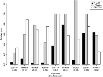
Table 1 lists the 18 existing haplotypes together with the estimates, by PHASE, LDPooled and GREEDY. The nature of our target distribution as an empirical distribution of a certain Markov chain makes it also straightforward to quantify the uncertainty in the estimates, and the 95%-probability intervals of the results given by PHASE are shown. The relative errors of the estimates (i.e. |e h−t h|/t h, where e h and t h are the estimated and true relative frequencies, respectively) are reported in Fig. 1 for the nine haplotypes whose true frequency was over 2%. In Table 1 and Fig. 1, the results of PHASE are from the run with the highest PAC-B likelihood (see the Appendix for details).
Relative errors of frequency estimates of nine most common haplotypes in the simulated example.
Frequency estimates on the simulated data set. The best estimate for each haplotype is shown in boldface
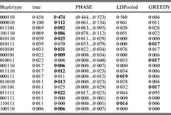
Ito et al. (Reference Ito, Chiku, Inoue, Tomita, Morisaki, Morisaki and Kamatani2003) reported that on their examples LDPooled gave rather accurate estimates of the major haplotypes (frequency at least 10% at population). In our example, it seems that PHASE can yield accurate results for such major haplotypes but for LDPooled and the greedy algorithm the relative errors, even for those major haplotypes, rise to about 80% (Fig. 1).
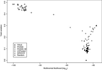
Table 2 lists the statistics of the variation distance between the estimates and the true distribution over 30 different runs. It seems that the convergence of the PHASE is not complete as there are some variations between the runs started from different initial states, but it is very much better than without the recombination model (PHASE-M). It can also be seen that in terms of the total variation distance, PHASE clearly outperforms the other methods. LDPooled is perfectly consistent in its maximum-likelihood estimate (all 30 runs are at the same distance from the truth), but this distribution seems to be relatively far from the true distribution, compared with the estimates given by PHASE. We have also studied the relation between the multinomial likelihood of the pooled data and the total variation distance to the true distribution more thoroughly in Fig. 2. There it can be seen that LDPooled gives haplotype frequency estimates whose multinomial likelihoods are the highest and in that sense LDPooled works exactly as expected. However, in terms of both total variation distances and multinomial likelihoods, the estimates of PHASE seem to be closer to the true distribution. In conclusion, it seems that the properties of the simulated process (meiosis on a fixed pedigree) are better captured by the model of PHASE than the multinomial likelihood.
Relation between multinomial likelihood and the total variation distance to the true haplotype distribution in the simulated example.
Distances to the true distribution on the simulated data set
(ii) HapMap data
The International HapMap Project (International HapMap Consortium, 2003, 2005, 2007) aims to catalogue the major (SNP) haplotype variation within and between several human populations. Currently, over 3·1 million SNPs from the human genome have been genotyped on 270 individuals originating from four geographically different populations. A valuable feature of the project is that it releases all the gathered information to the public domain. In the following examples we concentrate on one of the HapMap populations, Utah residents with ancestry from northern and western Europe (CEU population). For this population the database contains the estimated haplotype information on 30 trios (mother, father and their child) whose 60 parents are utilized in our analyses. The original procedure of the HapMap project was to use the genotypes of the children to estimate the haplotypes of the parents and if some ambiguities still remained, to apply PHASE (v.2.1) on the data. Because we are interested in estimating haplotype frequencies from population samples we do not utilize the data on the children of trios. Naturally, this makes our estimates less accurate than those of the HapMap database. In the following, we consider the results of the HapMap project as the ‘correct’ ones with which the accuracy of the results achieved on pooled samples are then compared. Indeed, the HapMap project has estimated that switch errors – where the phase of the adjacent marker loci is incorrectly inferred – occur extraordinarily rarely in CEU data sets: one error in every 8×10⁶ base pairs (International HapMap Consortium, 2005). There are ten so-called ENCODE regions in the HapMap database from which the HapMap project has extracted detailed information on common DNA variation. Each of these regions is about 500 kilobases (kb) long and they are spread over seven different chromosomes of the human genome.
In the following examples we consider three data sets collected from the ENCODE regions. E100 is extracted by including for each ENCODE region the first ten such markers that the physical distance between the adjacent markers becomes at least 100 base pairs. The other sets, E5k and E25k, are otherwise similar but the constraints imposed on the distances between the neighbouring markers are set to 5 and 25 kb, respectively. Table 3 contains more details of the marker spacing in these data sets.
Marker spacing (in base pairs) in HapMap data sets

(a) Effect of pool size on the accuracy of estimates
The most important question concerning the proposed method is the relationship between the accuracy of the haplotype frequency estimates and the pool size. It is clear that the accuracy decreases as the pool size increases, but how fast this happens depends on the particular data set.
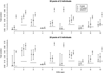
For the data sets E100 and E5k, we performed analyses with five different pool sizes: 2, 3, 4, 5 and 10 individuals per pool. Thus the corresponding number of pools in these settings was 30, 20, 15, 12 and 6, respectively. Each pool configuration was analysed 100 times, starting each time from a random initial state. The upper panels of Figs 3 & 4 show the distribution of the total variation distance of the estimates to the true distribution (HapMap database) and can be used to monitor the convergence of the algorithm. In the lower panels we have chosen one particular run out of each set of 100 replicates to represent our final estimate. This choice is made using the PAC-B likelihood criterion as explained in the Appendix. In order to validate the utilization of PAC-B likelihood, Fig. 5 shows that larger PAC-B likelihood values seem to imply more accurate estimates (smaller distance to the true distribution). The lower panels of Figs 3 and 4 also contain the levels of accuracy that are achieved when PHASE is applied to the same data but with pools of size 1 (black horizontal lines). We can see that pools of size 2 manage to give the same accuracy as pools of size 1 in almost all the cases and that with the data set E100 even the pools of size 5 give estimates that are very close to those from the pools of size 1.
Total variation distances from the estimated haplotype distributions on E100 to the true ones. The horizontal axis contains ten different genomic regions and for each the analyses are carried out for five different pool sizes (2, 3, 4, 5 and 10). For each region and each pool size, the upper panel shows the results of 100 separate runs. For the lower panel, a single run with the highest PAC-B likelihood has been chosen to represent the final estimate. The horizontal lines in the lower panel depict the results given by PHASE when run on single-individual pools. Pooling schemes are given in the form ‘Number of pools×Number of individuals per pool’.

Total variation distances from the estimated haplotype distributions on E5k to the true ones. The horizontal axis contains ten different genomic regions and for each the analyses are carried out for five different pool sizes (2, 3, 4, 5 and 10). For each region and each pool size, the upper panel shows the results of 100 separate runs. For the lower panel, a single run with the highest PAC-B likelihood has been chosen to represent the final estimate. The horizontal lines in the lower panel depict the results given by PHASE when run on single-individual pools. Pooling schemes are given in the form ‘Number of pools×Number of individuals per pool’.
Relation between PAC-B likelihood and total variation distance between true and estimated distributions. The results are shown for ten regions of E100 data sets for two pooling schemes: five individuals per pool (two upper lines) and ten individuals per pool (two lower lines). Each picture describes the results of 100 separate runs.

From the results with larger pool sizes (3, 4, 5 or 10) on the data set E5k, it is clear that in order to achieve reliable results, several runs are needed together with some monitoring of their likelihood values. The possible sources of the failure to convergence to a single haplotype distribution are considered in the Discussion section.
(b) Effect of pool size when the number of pools is fixed
In this example we show that analysing pooled data with PHASE can be effective when the goal is to have the most credible estimates of the population haplotype frequencies when only a fixed number of genotyping events can be carried out. At the same time, we also study the variability of the estimates when the compositions of pools are changed, i.e. when the group of individuals that are pooled together is varied.
As seen in the previous example, increasing the size of the pools decreases the accuracy of the estimates. On the other hand, small pools result in a small total number of analysed haplotypes, whence one is more likely to miss some properties of the whole population already due to a small sample size.
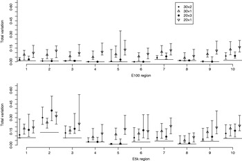
Fig. 6 illustrates the results for the cases where the number of pools is either 30 or 20, and where either all available samples are used (pool sizes of 2 and 3 individuals, respectively) or only a single individual is assigned to each pool. Each point in Fig. 6 denotes the median of the total variation distances of 20 pool compositions of the corresponding pooling scheme, and the interval around the median extends from the minimum to the maximum of those 20 total variation distances. For pooled data the PHASE algorithm was run 10 times on each of the 20 pool compositions, and the one with the highest PAC-B likelihood was considered as the final result.
In almost all the cases, pooling 2 or 3 individuals yields results that are closer to the frequencies in the HapMap database than analysing the same number of individuals (30 or 20, respectively) separately using the original PHASE algorithm. Thus, in those cases, the reduction in haplotyping accuracy caused by pooling several individuals is well compensated by the ability to analyse larger samples from the underlying population. Currently, the HapMap database includes only 60 (unrelated) individuals from CEU population and thus we have not made comparisons in situations where also the pooled samples would be just a subset of the whole population.
Total variation distances between the estimated haplotype distributions and the true ones. On the horizontal axis, there are ten different genomic regions and for each there are four different pooling schemes. For each region and each pooling scheme, 20 different pool contents were analysed and their results lie within the vertical intervals. Points represent medians of 20 analyses. The upper panel concerns the data set E100 and the lower panel the data set E5k. Pooling schemes are given in the form ‘Number of pools×Number of individuals per pool’.
(c) Performance comparisons between the methods
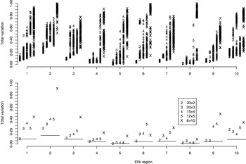
We were not able to run LDPooled on the data sets with ten markers, when there were more than 2 individuals per pool. Thus we decreased the number of markers to 7 and studied the accuracy of PHASE, LDPooled and the greedy algorithm on the data set E25k. For each ENCODE region and pool sizes of 2 and 3 individuals, 20 different pool configurations were analysed and the results are shown in Fig. 7. For both PHASE and LDPooled, each pool configuration was analysed 10 times, starting each time from a different initial haplotype configuration, and the estimate with the highest likelihood (PAC-B likelihood for PHASE and multinomial likelihood for LDPooled) was recorded. The results show that in the majority of the cases, PHASE has smaller median distance to the HapMap database than LDPooled, and both of them clearly outperform the greedy algorithm. The running time on a single region was on average 0·5 (pool size 2) and 36·6 (pool size 3) seconds for LDPooled, and for PHASE the corresponding analyses took about 25 min, independently of the pool size.
Total variation distances between the estimated haplotype distributions and the true ones on the data set E25k. On the horizontal axis, there are ten different genomic regions and for each combination of region, method and pooling scheme, 20 different pool contents were analysed. The results lie between the vertical intervals and points represent medians of 20 analyses. Pooling schemes are given in the form ‘Number of pools×Number of individuals per pool’.
4. Discussion
The haplotyping problem – to estimate the two multilocus allelic combinations of each sampled individual from their unphased genotype data – has been studied extensively in the literature (Niu, Reference Niu2004), because haplotype information is valuable in many genetic analyses. On the other hand, current technology allows us to pool DNA from several individuals and estimate reliably the allele frequencies of the whole pool at one genotyping, thus reducing the overall genotyping costs (Sham et al., Reference Sham, Bader, Craig, O'Donovan and Owen2002). One disadvantage of the pooling techniques is that an increase in the pool size results in a decrease in the haplotype information. In this article, we have studied to what extent it is possible to reveal the haplotype configurations from the pooled allelic information of several diploid individuals.
Several earlier studies have relied on the numerical maximization of the likelihood function that arises from the multinomial sampling model of the haplotypes (Ito et al., Reference Ito, Chiku, Inoue, Tomita, Morisaki, Morisaki and Kamatani2003; Wang et al., Reference Wang, Kidd and Zhao2003; Yang et al., Reference Yang, Zhang, Hoh, Matsuda, Xu, Lathrop and Ott2003). Recently, that approach was also improved by several pre- and post-processing steps of the SNP data (Kirkpatrick et al., Reference Kirkpatrick, Armendariz, Karp and Halperin2007). Here, we extended the current state-of-the-art method for population-based haplotyping of individual data, the PHASE algorithm (Stephens & Scheet, Reference Stephens and Scheet2005), to the setting of pooled data, and compared the results with the maximum-likelihood estimates given by LDPooled (Ito et al., Reference Ito, Chiku, Inoue, Tomita, Morisaki, Morisaki and Kamatani2003) and with a deterministic greedy algorithm.
There are two appealing properties of PHASE that encouraged us to apply it to the pooled data. The first is of course the top performance of PHASE in the extensive comparisons carried out among several haplotyping methods (Marchini et al., Reference Marchini, Cutler, Patterson, Stephens, Eskin, Halperin, Lin, Qin, Munro, Abecasis and Donnelly2006). The second is the simplicity in the modifications that are needed in order to extend the algorithm to pooled data. The PHASE algorithm conducts a series of iterations through the space of possible haplotype configurations of the individuals given their genotype data. Hence, it is straightforward to introduce an additional step between consecutive iterations that randomly pairs the current haplotypes within each pool and thus permits the algorithm to explore the whole space of the possible haplotypes given the pooled data. The original PHASE algorithm can be seen as a version of the extended algorithm where the pool size equals 1. As PHASE estimates also the recombination fractions for each marker interval, the same could also be done when the algorithm is applied to the pooled data.
Computationally, the PHASE algorithm is based on the ideas from the theory of MCMC computing. Nevertheless, PHASE (v.2.1) lacks a rigorous theoretical basis since it has not been proved that there exists an underlying haplotype distribution towards which the algorithm converges (Niu et al., Reference Niu, Qin, Xu and Liu2002; Stephens & Scheet, Reference Stephens and Scheet2005). However, to our knowledge, no such problems in practice have been reported in the literature. This being said, we found out that in more complex pooled data cases, our modification of the algorithm failed to converge to a single distribution within the given number of iterations. A possible explanation for this could be multimodality of the (assumed-to-exist) target distribution together with the extremely local updates performed by Gibbs sampler. Indeed, since the algorithm updates only a single pair of haplotypes at a time, it may not move from a local mode of the distribution once it reaches there. The same should be true with the original PHASE algorithm, but since the number of possible haplotype combinations increases dramatically as the pool size grows, it may be that these problems are not likely to emerge on single-individual pools. A possible solution might be updating more haplotypes simultaneously at each MCMC step (e.g. updating a whole pool at a time). Unfortunately, this would be computationally more demanding. Another possible explanation for the observed convergence problems could be insufficient number of iterations carried out in our examples. However, we consider the multimodality of the vast state space of consistent haplotype configurations as the most likely source of these problems, because it seemed that the posterior distributions of the runs did not vary much anymore after those 100 PHASE cycles (see the Appendix) that were reported in our results. This was noticed when some of the runs were extended some hundreds of PHASE cycles longer (results not shown).
To overcome the convergence issues, we discovered that the PAC-B likelihood value reported by PHASE can very effectively rank different distributions, since a high likelihood value seems to indicate lower distance to the correct result (see Fig. 5). This led us to run many small runs rather than a single long one in our examples. Thus we consider the proposed procedure not as a proper MCMC method but more like a search algorithm through a set of modes of the distribution that are ranked according to their accordance with a reasonable genetic model (PAC-B likelihood).
In our examples we found out that in order to have accurate results the pool size needs to be quite small, 2–5 individuals per pool, depending on the data set. This is in line with the earlier studies where at most 3 (Kirkpatrick et al., Reference Kirkpatrick, Armendariz, Karp and Halperin2007) or 4 individuals per pool are reported to yield optimal efficiency (Ito et al., Reference Ito, Chiku, Inoue, Tomita, Morisaki, Morisaki and Kamatani2003; Yang et al., Reference Yang, Zhang, Hoh, Matsuda, Xu, Lathrop and Ott2003). There are a few immediate ways to increase the pool size by influencing the information content of the pools. Firstly, one might try to minimize the variability within each pool, whence the pool size could be increased as the number of possible combinations of haplotypes in each pool would decrease. Here observed information on covariates or prior information on the known family or population structure could be utilized by pooling closely related individuals. Another way to increase the pool sizes would be to include in the model some prior information on the population haplotype distribution that has been gathered from some previous studies or a public database like the HapMap project. This might effectively decrease the number of likely haplotype combinations within the pools, and thus also improve the efficiency and the convergence of the algorithm. A shortcut for implementing this idea in the modified version of PHASE would be to add some pseudo-individuals to the data. These artificial genotypes would be homozygous for some haplotypes that are known to exist in the population. As a result the algorithm would not spend time updating these homozygous pseudo-individuals, whereas the Gibbs update step of the unknown pooled haplotypes would be altered by putting more weight on the artificially added haplotypes.
The proposed modification of PHASE to pooled data is very flexible with respect to the compositions of pools. Indeed, there are no technical constraints limiting the pool sizes, as for the fixed number of haplotypes the running time per iteration and memory requirements remain the same independently of the number of haplotypes per pool. This is opposite to the strong growth of memory requirements as a function of pool size in the EM algorithm implemented in LDPooled. One must keep in mind, however, that in order to get accurate results with PHASE, larger pools require more and/or longer runs than small ones.
Both PHASE and LDPooled can analyse pools of different sizes at the same run. For more difficult data sets it may be useful to utilize the pooling techniques only to a part of the data and genotype the remaining individuals separately. We compared for example the following pooling schemes on HapMap data: 30×2, 10×1+10×2+10×3 and 20×1+10×4. Each scheme considers 30 pools and 120 haplotypes but the pool sizes vary from 1 to 4 (individuals per pool). The estimates of the different schemes were so similar to each other that in this article we have reported only the basic versions with the constant pool size (here 30×2).
In our examples we concentrated our efforts on producing comprehensive results by studying several different regions from the human genome and by assessing the effects of the pool assignment of the individuals by repeating each analysis several times with varying pool composition. On the other hand, our examples did not consider more than ten markers at a time. The reason for this is that for computational reasons the current approach to haplotype estimation on larger sets of markers with PHASE (or with the multinomial model) proceeds through the partition-ligation steps (Niu et al., Reference Niu, Qin, Xu and Liu2002). There only small regions (tens of markers) are analysed at a time and only afterwards these regions are combined to cover the whole haplotypes. Thus the essential part of the kind of haplotyping algorithms we have studied here is in estimating the haplotype patterns in small segments.
The simple greedy algorithm was presented for testing the complexity of the data sets. In the HapMap data sets the greedy method performed clearly much worse than PHASE and LDPooled. For the data set E25k, this can be seen in Fig. 7 and the same pattern was also present for the data sets El00 and E5k (results not shown). In the simulated data set, we used the greedy algorithm to guide our choice of the distance between markers. For very close markers the greedy method seemed to yield similar results to PHASE but for the data set reported in Table 1 and Fig. 1, this was no longer the case. While testing the method we also experimented using the haplotype frequencies given by the greedy algorithm as starting values for PHASE. However, this led to the mixing problems of the MCMC chain. A potential reason for these problems is that the greedy method has maximized the number of certain haplotypes given the allele frequencies in the pools. This may prevent the Gibbs updates of the PHASE algorithm to move away from the greedy configuration, because these updates sample only two haplotypes at a time conditional on the other haplotypes.
The comparisons of accuracy between PHASE and LDPooled did not yield a completely consistent conclusion. On the simulated data set PHASE performed much better but from the HapMap data a few regions were found on which LDPooled was the superior method (e.g. E25k – region 6–30 pools and E25k – region 7–20 pools). However, in most of the cases reported in Fig. 7, PHASE had an advantage over LDPooled. Because of insufficient memory, LDPooled was not able to analyse HapMap data sets with ten markers for pool sizes larger than 2. For pool size 2, PHASE and LDPooled gave similar accuracy on E100, and PHASE had a slight advantage on E5k (results not shown). On the other hand, when memory was not a problem, LDPooled was faster than the procedure involving PHASE. We also note that Kirkpatrick et al. (Reference Kirkpatrick, Armendariz, Karp and Halperin2007) have reported that their program HaploPool outperforms LDPooled both in accuracy and in speed. Comparisons between PHASE and HaploPool will remain a question for further study.
From Figs 6 and 7, we can conclude that an assignment of the individuals to the pools has a stronger effect on the accuracy of the results when the distance between the SNPs is larger. For E100 the pool composition has a negligible role in the accuracy (except in region 5), whereas for E5k and especially for E25k, different pooled combinations of individuals result in very different accuracy of the estimates. In these examples, the PHASE algorithm was run only 10 times for each data set and, as is apparent from Fig. 5, the results might be improved if 100 or even more repetitions per pool composition were conducted. On the other hand, as Fig. 6 shows, the same kind of variability of the accuracy is also present in the case where only a subset of the subjects is analysed individually. Thus pooling can be advantageous also in cases where one has to compromise between the number of genotypings (i.e. pools) and the number of analysed samples, as is the case with the example of Fig. 6.
There are two sources of errors related to the haplotyping problem on pooled data which we have partially ignored in this study. Firstly, there is sampling error occurring because only a subset of the whole population is usually utilized in the studies. Secondly, there are certain sources of genotyping errors in the pooling techniques which may affect the accuracy of the estimated allele frequencies of pools. The question of sampling error was considered in the examples of Fig. 6 for single-individual pools, but the relatively small number of individuals (60) in the HapMap database made us refrain from studying the issue for larger pools. Since we study relatively small pools (2–5 individuals), the proportion of each allele in a pool has only a few possible values that are clearly distinct from each other. As several pooling technologies generally give the allele frequencies within the accuracy of 5% or less (Sham et al., Reference Sham, Bader, Craig, O'Donovan and Owen2002), we are not expecting the accuracy of the techniques to be a considerable problem in this setting. Kirkpatrick et al. (Reference Kirkpatrick, Armendariz, Karp and Halperin2007) studied the effect of perturbation of the allele frequencies of pools by Gaussian noise and found that their program HaploPool (pool size 2) was advantageous over single-individual genotyping as long as the standard deviation of the noise was less than 0·05. Also in the setting of Quade et al. (Reference Quade, Elston and Goddard2005) the genotyping error did not have a serious effect on the accuracy of the haplotype frequency estimates, although one must keep in mind that their study considered only the case of two SNPs.
In conclusion, our results show that pooling may be efficient on data sets like E100, where even pools of size 5 (individuals per pool) seem to give almost equal accuracy of the population haplotype frequencies as ordinary single-individual analysis (Figs 3 and 6). Obvious challenges for our approach still remain concerning the convergence issues encountered in more complex data sets. We hope that our idea of using PHASE on pooled data encourages more research on these issues and that some further modifications of the algorithm can bring robustness to the method. Important topics for future work also include incorporating external information of population haplotype distribution into the model, considering the settings where the exact sizes of the pools are unknown (e.g. in forensic genetics), and modelling genotyping errors, especially for larger pools. Furthermore, the extendibility of other promising haplotyping methods to the pooled DNA data as well as comparisons between the method presented here and HaploPool software of Kirkpatrick et al. (Reference Kirkpatrick, Armendariz, Karp and Halperin2007) are important issues requiring some further study.
We are grateful to Matthew Stephens for providing the source codes of PHASE and to Toshikazu Ito for the program LDPooled and also to two anonymous reviewers whose comments helped us to improve the manuscript. This work was supported by research grant numbers 114786, 122883 and 202324 from the Academy of Finland and the ComBi Graduate School.
Appendix: Implementation and parameters
As described in the Methods section, our modified version of PHASE (v.2.1) for pooled data proceeds by (i) forming for each pool i randomly n i pairs of haplotypes from the 2n i haplotypes present in the pool and (ii) applying the transition kernel of PHASE (R times) to these paired haplotypes. In the following, we shall call the part (ii) a PHASE cycle.
Once a new PHASE cycle is commenced, we must also transfer the final recombination parameters ρ from the previous cycle to the new one. This can be done by implementing a function which reads in the parameters written by the function OutputRho(). Note that PHASE includes a switch (−i2) which allows us to input the genotype data in such a way that the given haplotypes are preserved between the PHASE cycles.
There are also parameters σp and σl that control the sizes of the updates of recombination parameters. These could also be transferred between the adjacent PHASE cycles, but we found it better to let the PHASE algorithm tune these parameters at the beginning of each PHASE cycle. This can be done by introducing some burn-in iterations into each PHASE cycle.
The results reported in this article have been produced by setting R=10 and using two burn-in iterations at the beginning at each PHASE cycle. We also tried the values R=5 and R=25 but the differences were very small (with some advantage for R=10). The number of PHASE cycles conducted in the simulated data example was 1500, whereas for the HapMap data sets the corresponding figure was 100. For each run the first 50 PHASE cycles were discarded as a burn-in part. On the HapMap data, the executed time by a single analysis (100 PHASE cycles with R=10 and 2 burn-in iterations on a single ENCODE region) was about 2·5 min (Pentium 4, 2·80 GHz). We note, however, that in order to get reliable results, several runs must be conducted (100 and 10 repetitions were used in our HapMap examples) and their consistency should be evaluated. In order to monitor the convergence properties of the chain, the original PHASE algorithm reports two quantities: the pseudo-likelihood of Stephens & Donnelly (Reference Stephens and Donnelly2003) and the PAC-B likelihood (Li & Stephens, Reference Li and Stephens2003). These can be thought of as providing a measure of the goodness of fit of the estimated haplotypes to the underlying model. We utilized these quantities because the runs with larger pool sizes (>3) were not converging to a single distribution (within the given time) and thus it did not seem reasonable to average the results over different runs. Instead, we ranked the runs according to their average values of PAC-B likelihoods and chose the run with the highest PAC-B likelihood to serve as our final estimate of the haplotype distribution. PAC-B likelihood was used because it was found to perform better in this task than the pseudo-likelihood. Its name abbreviates ‘product of approximative conditionals’ and version B has been modified from version A using empirical results to correct the bias that was observed in version A (Li & Stephens, Reference Li and Stephens2003). The same function is also used by PHASE to provide the likelihood of recombination parameters given the haplotypes (eqn 2 in this article).
Our philosophy was to keep the modifications to the PHASE code as small as possible: only inputting ρ at the beginning of each PHASE cycle and outputting ρ and the current haplotypes at the end of the cycle. In addition to these changes to the PHASE code one also needs helper programs that (i) shuffle the haplotypes within pools after each PHASE cycle and (ii) combine the results of the different PHASE cycles.


