


Introduction
Efficiency estimation is a popular way of assessing farm performance and numerous applications exist within the agricultural economics literature. Building on a microeconomic model of the farm, efficiency analysis is based on the estimation of an efficient isoquant or production possibility frontier. Irrespective of approach, the efficient frontier is estimated empirically based on available data. Following this, the position of each farm relative to the efficient frontier is assessed and possible deviations are considered inefficiency (Coelli et al., Reference Coelli, Rao, O'Donnell and Battese2005). Previous literature has not only been interested in the level of inefficiency but also in the impact of characteristics of the farm and farmer and/or the policy environment in which the farm exists. Common applications include an interest in personal characteristics of the farmer (Galanopoulos et al., Reference Galanopoulos, Aggelopoulos, Kamenidou and Mattas2006; Puig-Junoy and Argiles, Reference Puig-Junoy and Argiles2004), financial management (Davidova and Latruffe, Reference Davidova and Latruffe2007), management control (Manevska-Tasevska and Hansson, Reference Manevska-Tasevska and Hansson2011; Trip et al., Reference Trip, Thijssen, Renkema and Huirne2002), management routines and practices (Labajova et al., Reference Labajova, Hansson, Asmild, Göransson, Lagerkvist and Neil2016; Rougoor et al., Reference Rougoor, Trip, Huirne and Renkema1998), and agricultural subsidies (Latruffe and Nauges, Reference Latruffe and Nauges2013). The literature has also suggested existence of rational inefficiency, meaning that firms deliberately position themselves seemingly inefficiently in production possibility space because they get something out of this that is not observable in a standard production economic framework (Asmild, Bogetoft, and Hougaard, Reference Asmild, Bogetoft and Hougaard2013; Bogetoft and Hougaard, Reference Bogetoft and Hougaard2003; Hansson, Manevska-Tasevska, and Asmild, Reference Hansson, Manevska-Tasevska and Asmild2020).
Empirical efficiency estimations of agricultural production require access to data on production features at farm level based on which production inputs and outputs can be quantified. In applications based on farms in various European Union member states, efficiency studies are normally based on data obtained from the nationally available farm economic surveys where accounting data from a sample of national farmers are available. Examples include work by Hansson et al. (Reference Hansson, Manevska-Tasevska and Asmild2020) and Manevska-Tasevska, Hansson, and Labajova (Reference Manevska-Tasevska, Hansson and Labajova2017) for Sweden; Henningsen et al. (Reference Henningsen, Czekaj, Forkman, Lund and Nielsen2018) for Denmark; and Latruffe and Nauges (Reference Latruffe and Nauges2013) for France. This type of data usually originates from the Farm Accounting Data Network (FADN) as in Latruffe and Nauges (Reference Latruffe and Nauges2013) or originates from other data sources, which countries collect to feed into the FADN. One example is the Farm Economic Surveys (FES) in Sweden as in Hansson et al. (Reference Hansson, Manevska-Tasevska and Asmild2020) and in Manevska-Tasevska et al. (Reference Manevska-Tasevska, Hansson and Labajova2017), which function as the national background data for the FADN variable construction.
These types of accounting datasets generally give access to detailed accounts in the balance sheet and income statement of participating farmers, or to economic variables constructed from accounting data, and to some additionally collected data such as number of hectares operated by the farm and hours worked at the farm. They are convenient for research in the sense that they are easily accessible to researchers, provide information that is representative of various farming systems using standardized methods, and is well-known to many researchers.
However, while offering many benefits for researchers, accounting-based datasets are also associated with inherent drawbacks for the construction of production economic datasets needed for efficiency analyses. This is due to the fact that most of the variables in the datasets are expressed in monetary terms. This means that in practice, most production inputs and outputs in efficiency analyses are in fact only approximated using measures of production costs and production revenues in various categories. In some regions and datasets, there exist price indices that can be used to approximate quantities; however, the accuracy of this for individual observations cannot be guaranteed. Considering how accounting-based datasets are compiled, quantities of production inputs and outputs cannot be properly disentangled from prices. This means that researchers may compare farms that use larger quantities acquired for low prices (larger quantities of output sold for low prices) with farms that use smaller quantities acquired for higher prices (smaller quantities of output sold for high prices) and consider them similar in terms of input use (output production) even though they may use (produce) different quantities. Considering the fact that higher prices normally can be taken to signal higher quality, this becomes even more intriguing because the information cannot be used to distinguish between observations with high-quality inputs and outputs from those with low-quality inputs and outputs, although they are, as signaled by the quality differences, likely to operate under separate technologies. In particular, it is common in agriculture that farmers are paid according to the quality of their produce, for instance, the fat and protein content of their milk, or according to the quality of their grain. Still from the accounting data, the possible quality differences highlighted by differences in prices cannot be disentangled. Exceptions to the quantity dilemma are production factors of the type of agricultural land and labor, which are normally expressed in hectares and hours, respectively. However, these variables are not accompanied by information about prices paid for those production factors or with information about their opportunity costs.
Being by large based on monetary measures of production inputs and outputs, which are composed of quantities and prices, efficiency studies based on accounting data in practice inevitably assess a mix between what could be considered technical efficiency (relating to the correspondence of quantities used and produced) and allocative efficiency (relating to the correspondence of prices paid and received). Both the technical component and the allocative component are intervened in the final measure, making it unclear what is actually being measured. This introduces conceptual uncertainties about what has actually been measured. Moreover, the use of monetary variables where quantities and prices are mixed may affect the size of the estimated efficiency scores, as well as the rankings of farms according to the scores, hence introducing a bias to the final efficiency assessment. As a consequence, conclusions may be unclear or even misleading, and this can complicate policy advice based on efficiency analyses. However, based on previous research, it is not clear to which extent efficiency results may be affected by the use of data that mixes quantities and prices to proxy production economic data.
The purpose of this study is therefore to investigate empirically the role of data type in efficiency estimation. We do this by evaluating and illustrating the extent to which conclusions in terms of distributions of farms from the most to the least efficient are affected by estimation of efficiency based on quantities of production inputs and outputs or on costs and revenues. We base the analysis on a farm-level data set from the 2015 Ethiopia Rural Socioeconomic Survey (ERSS) (World Bank, Reference World Bank2016), which by construction contains information about production inputs and outputs in quantities as well as production input and output prices. This allows us to estimate and compare efficiency scores based on i) quantities and ii) mostly expenses and revenues (i.e. a variable specification similar to that allowed by the FADN and FES datasets in Europe). In doing so, we provide empirical insights into the possible bias introduced by not having access to production quantities and prices as is the case in most efficiency studies based on European data.
It should be emphasized that the dataset used in this study represents a farming system that is very different from that of most European countries. It should therefore be acknowledged that conclusions about the magnitude of the possible problem are dependent on the dataset we use; other datasets may indicate a smaller or larger problem. Having said that, our study makes a novel contribution to the literature by being the first to acknowledge and provide empirical evidence about the potential bias in efficiency estimation introduced by basing efficiency studies by large on cost and revenue data instead of on quantity-based data and prices. In doing so, we provide a useful basis for discussing the usefulness of using price information to calculate production factors and outputs when such data is available and of extending current accounting-based datasets to include also price information, which would allow for calculating input and output quantities. We also provide a basis for a more careful discussion about what type of efficiency measures are actually obtained from variables that are largely based on costs and revenues and thus contain elements of both quantities and prices.
Background – exploring the problems with efficiency assessment based on accounting data
The conceptualization of firm efficiency has long historical roots and goes back to work by Farrell (Reference Farrell1957). After Aigner et al. (Reference Aigner, Lovell and Schmidt1977) and Meeusen and van den Broeck (Reference Meeusen and van den Broeck1977) provided the basis for an econometric framework to estimate efficiency, and Charnes et al. (Reference Charnes, Cooper and Rhodes1978) provided a nonparametric approach based on mathematical linear programing, there have been numerous applications across scientific fields and examples include Bokusheva et al (Reference Bokusheva, Hockmann and Kumbhakar2012) Mardani et al (Reference Mardani, Zavadskas, Streimikiene, Jusoh and Khoshnoudi2017) and Nauges et al (Reference Nauges, O'Donnell and Quiggin2011).
The efficiency concept starts from a microeconomic model of the firm where it is assumed that the firm uses production factors (x) to produce outputs (y), given technology T (e.g. Coelli et al., Reference Coelli, Rao, O'Donnell and Battese2005). Production factors can be obtained at price (w) and outputs sold at price (p). The efficient use of production factors and production output can be determined from the production possibility set. Deviations from the efficient use of production factors at a given level of production output are considered inefficiency. The literature has suggested many reasons for inefficiency as introduced above.
Three types of efficiency are generally distinguished: Technical efficiency (TE) considers the potential inefficiency in a firm’s use of production factors given a certain level of production output (input case) or in a firm’s production output given a certain level of production factors (output case). Allocative efficiency (AE) considers the potential inefficiency in a firm’s combination of production factors given factor prices (input case) or in a firm’s combination of production outputs given the product output prices (output case). A combination of TE and AE measures the economic (or overall) efficiency (EE) from the input or output perspective. The literature has suggested more advanced efficiency models, including dynamic efficiency (Nemoto and Goto, Reference Nemoto and Goto2003; Tsionas, Reference Tsionas2006), however, it is out of the scope of this paper to review these in detail; our focus is on demonstrating the possible impact caused on efficiency scores by the type of data aggregation used.
Empirical assessment of TE, AE, and EE requires access to information about firm’s use of production factors and production of outputs in quantities, as well as information about prices per unit of production factors and production outputs. Because this is not available for all production factors and production outputs in most accounting-derived datasets upon which efficiency studies are based, production factors and production outputs are proxied by information about costs and revenues obtained by firms. In effect, this means that production factors in many cases are considered in terms of (x * w) and production outputs in terms of (y * p). In effect, this means measuring how well firms can transform a set of costs acquired by the use of various production factors into a set of revenues obtained from selling a set of production outputs. This implies that it is not possible to distinguish between inefficiency in use of production factors from inefficiency in combination of production factors (or combinations of production outputs). As a result, it is not possible to distinguish technical and allocative inefficiencies from the overall economic efficiency. Furthermore, firms with different strategic approaches are considered similar, although it would be more feasible to consider them as operating under different technologies. In fact, it is not possible to distinguish between a firm that uses smaller amounts of production factors, but acquired them at a higher price from a firm that uses larger amounts of its production factors, but acquired them at a lower price. Likewise, it is not possible to distinguish between a firm that produces (and sells) a small amount of production output, but at a higher price per unit from a firm that produces (and sells) a larger amount of production output but at a lower price per unit. As a result, efficiency results and rankings of firms according to inefficiency are possibly biased.
It should be noted that in competitive markets with perfect information flows prices will be the same for all firms. In such markets, the cost function can be derived from the production function and the production function can be derived back again from the cost function, using the duality between production and cost functions. The potential bias in efficiency estimation that we are pointing to in this paper would not exist in such markets. Notably, the possible bias that we are pointing to is dependent on the degree to which firms can affect prices through various choices. In cases where prices are homogeneous, the possible bias in technical input and output efficiency would be less severe; all firms encounter the same prices and differences in expenses and revenues should indeed represent differences in the amount of production factors used and the amount of output produced. However, in many cases, input and output prices can be affected through possible various strategic choices such as type of employee categories and use of various contracts to fix output prices in advance. Prices may also differ due to differences in negotiation skills, for instance between men and women. Furthermore, prices may also vary between different regions in the same country. However, based on common production economic data, such heterogeneity between farms cannot be revealed and considered in efficiency studies.
Method and data
Data
To investigate the role of data in efficiency estimation, this study uses a farm-level dataset from the 2015 ERSS obtained from all regions in Ethiopia (World Bank, Reference World Bank2016). This data compiles a set of information on farm household socioeconomic characteristics, crop and livestock production, agricultural input use, community-level output and input prices, employment, farm, and non-farm income. Specifically, through this dataset, we were able to separate quantities of production factors and outputs and prices. In particular, we used production variables including main crop harvest, land, labor, fertilizer use, average wage rate, and output prices to estimate the input-oriented technical efficiency level. Our analysis considered the village-level prices as a farm gate price given the case that rural farmers in Ethiopia usually sell main crops in the nearby village markets.
Summary statistics of outputs, production factors, and prices are provided in Table 1. Production factors were specified as land, labor, and fertilizer use. The output variable was represented by a total harvest index, which was constructed by summing the quantity of major crops weighted by the prices. The considered crops were Barley, Maize, Millet, Sorghum, Wheat, and Teff (Eragrostis tef). The corresponding mean value of the total harvest index is 14.65 with a standard deviation of 241.42.
Table 1. Summary statistics for the key variables
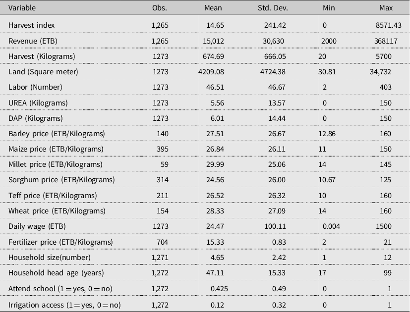
The average household landholding is around 4209 square meters (≈0.42 hectares), while labor use represented by the number of days in a year is 46.51 days/harvest season. A similar figure was reported in other studies (e.g., Tirkaso and Hess, Reference Tirkaso and Hess2018). The use of chemical fertilizer is relatively small. For instance, each household uses an average of 5.56 and 6.01 kg of UREA and DAP, respectively, on their farm during the planting season. The price level for each crop’s outputs and inputs are also presented. Therefore, after consideration of missing values and outliers, we retained a total of 1273 farm households in our analysis.
Measurement errors in surveys present a recurring challenge, resulting in significant bias in econometric and statistical analyses. For example, data provided by farmers, including agricultural income, input costs, and other production-related expenses, often suffer from inaccuracies due to underreporting or overreporting. To address these potential pitfalls, the enumerators of the ERSS underwent six training sessions before conducting the survey (World Bank, Reference World Bank2016). Furthermore, competent field supervisors were assigned to oversee the survey at the field level, ensuring the precision of the collected data. This comprehensive approach helps to minimize potential measurement errors during the survey.
Analytical strategy
Most empirical works in production economics use the duality theorem to derive the cost function from the corresponding production function, establishing a mathematical link by applying the duality theorem. While this approach could provide a strong theoretical foundation for the analysis, there are certain limitations to its applicability in our context. For example, it may not be suitable in cases of imperfect markets, where information flow and regulatory constraints are dominant. Agricultural markets in developing countries including Ethiopia are mostly prone to market imperfections, where asymmetry of information, imperfect competition, externalities, and related phenomena are common (e.g., Hoddinott, Headey, and Dereje, Reference Hoddinott, Headey and Dereje2015; Osborne, Reference Osborne2005; Tirkaso and Hailu, Reference Tirkaso and Hailu2022). This indicates that the duality approach may not be sufficient to explain the complexities of agricultural markets in developing countries and other imperfect market conditions.
We approached the study objective by investigating how using data that are aggregated from quantities and prices into costs and revenues affects the distribution of farms from the most efficient to the least efficient. Thus, we ask if using costs and revenues instead of quantities to construct measures of production factors leads to differences in conclusions with respect to which specific observations are considered the more efficient and not – i.e. the ranking from the most inefficient to the least inefficient observation. To this end, we estimated efficiency scores under two scenarios: i) a quantity-based scenario (QBS), with production factors and outputs measured in quantities, and ii) a cost-revenue-based scenario (CRBS) where production factors and outputs are proxied using information about costs and revenues. All data used for the efficiency estimations are based on information about quantities and prices, so the estimations under the two scenarios can indeed be related and compared; based on the available information the data for the QBS scenario is based on quantities and information for the CRBS scenario is based on quantities multiplied with prices.
We further estimated each farms’ efficiency score by classifying the sample into whole sample, nontraditional farms (those who use chemical fertilizers such as UREA and DAPFootnote 1 ), and traditional farm categories (those farmers who do not use any of the chemical fertilizers). This provides an insight into how efficiency estimated under the two scenarios is distributed across different farm groups.
We use the nonparametric Data Envelopment Analysis (DEA) (Charnes et al., Reference Charnes, Cooper and Rhodes1978) to estimate efficiency scores of individual observations and use this to evaluate how type of data affects conclusions about the efficiency of each observation. Our specific empirical strategy follows the conventional radial Debreu-Farrell measure of efficiency loss (Debreu, Reference Debreu1951; Farrell, Reference Farrell1957), which assumed that for each data point k (k = 1,….,K), vector x k = (x k1 ,…,x kN ) ϵ R N represents N inputs, vector y k = (y k1 ,…,y kM ) ϵ R M indicates M outputs. We also assumed that under the technology representation, T, the data set (y, x) is producible by inputs:
 $$T = \{ (x,y):y\;{\rm{are}}\;{\rm{producible}}\;{\rm{by}}\;x\} $$
Further, the technology set is fully characterized by its input requirement set as follows:
 $$L(y) \equiv \{ x:(x,y)\varepsilon T\} $$
Equation (2) indicates all the available inputs and outputs are feasible. The magnitude of efficiency score is given by the difference between the distances of the upper boundary of the production possibility set and the lower boundary of the input requirement. Thus, we followed the input-oriented radial efficiency measurement approach that represents how much input quantities be proportionally decreased without changing the output quantity set, L(y). Consequently, empirically estimable radial Debreu – Farrell input-based measure of technical efficiency can be obtained by solving the linear programing problem for each data point k (k = 1,…, K) as follows:
 $${RM_{k}^{i}}(\,{y_{k}}, {x_{k}}, {y}, {x|CRS})=max\left\{{N^{-1}}{\sum\limits_{N=1}^{N}}{\lambda_{n}}:({\lambda_{1}}{x_{k1}},\ldots,{\lambda_{N}}{y_{kN}})\,\epsilon\, L(y), {\lambda_{n}}\geq 0, n=1, \ldots , N\right\}$$
where y is K × M matrix of available data on outputs and x is K × N matrix of available data on inputs. Based on equation (3), the radial measure expands all M outputs y k = (y k1 ,…, y kM ) (N inputs x k = (x k1 ,…,x kN )) proportionally until the frontier is reached for each data point (y k , x k ). The assumption regarding global technology is crucial in DEA estimation as the efficiency scores are sensitive to the underlying assumption. We first followed a constant return to scale technology (CRS) assumption and later econometrically tested whether the underlying assumption is appropriate or not. In the case where the CRS is not feasible, we rely on the variable return to scale technology (VRS) assumption.
Results
We present DEA estimates based on different sample classifications, i.e., the whole sample, nontraditional, and traditional farms.Footnote 2 We group those farmers using chemical fertilizers such as nitrogen and phosphorus as nontraditional farms, while the others are considered traditional. This classification allows us to examine the technical efficiency within each group. However, it should be noted that the technical efficiency scores cannot be directly compared across the groups, since the magnitude of the estimated scores is always impacted by the sample size; thus the individual efficiency scores within each group should only be interpreted in relation to the particular efficient frontier in focus. We presented estimates based on both CRS and VRS technology assumptions. In the case of CRS, we assumed for the production technology, this is equivalent to switching from output to input-oriented efficiency, while for variable VRS assumption, this one-to-one correspondence does not hold (Badunenko and Tauchmann, Reference Badunenko and Tauchmann2018).
Variable return to scale (VRS)
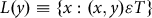
In the QBS, where we base the efficiency estimates on quantities of production factors and produced products (summarized into an index to allow for single output variable), our estimate for the whole sample shows an average technical efficiency score of 68.4% (Table 2). However, using the CRBS and basing the efficiency estimates on costs and revenues as proxy variables for quantities, provides an efficiency score of 72.2%. Similarly, the DEA estimates for nontraditional farmers show variation in the efficiency score with an average efficiency score of 68.9% under the QBS; whereas the average efficiency score amounts to 73.5% under the CRBS when price information is not considered and efficiency is instead based on expenses and revenues. There is also a difference in the average efficiency scores of traditional farmers when comparing scores based on quantities (the QBS) on the one hand and revenues and expenses on the other hand (the CRBS) (67.8% and 71.1%, respectively).
Table 2. Summary of DEA estimates by farm category under VRS
Note: CRBS refers to TE scores estimated from expenses and revenues; QBS refers to TE scores estimated from quantities of production factors and output as calculated using available price information.
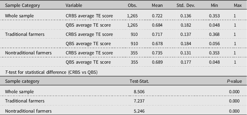
It can also be noted that the average efficiency score for nontraditional farmers is higher than that of the traditional farmers. This could be linked to the fact that nontraditional farmers utilize chemical fertilizers and other chemical compounds to increase farm yield, while the traditional farmers mainly use natural fertilizers such as manure and compost on their farms. We further examined whether there is statistically significant difference in the estimated technical efficiency score under the QBS and CRBS specifications. This was confirmed for all groups (p-values <0.000). The distributions of efficiency scores for each sample group are presented in Figure 1. The plots for CRBS and QBS under each sample category show variation with a right-skewed half-normal distribution.
Figure 1. TE distributions for CRBS and QBS under variable return to scale assumption.
Constant return to scale (CRS)
In the case of CRS assumption, the DEA estimate shows a considerably lower technical efficiency score (Table 3). For instance, under the QBS, the average whole-sample technical efficiency score is 66.2% when based on quantities of production factors and output; using expenses and revenues, under the CRBS, the average technical efficiency score amounts to 65.8%. The corresponding average figures for the nontraditional farmers are 56% and 61.8%, respectively. For the case of traditional farms, the corresponding efficiency score is 46.5% and 45.9%, respectively. We also tested whether there is a statistical difference in the estimated technical efficiency score between CRBS and QBS specifications. The difference was not significant for the whole sample and for the traditional farms, but for the nontraditional farmers, the difference was significant at general levels of significance.
Table 3. Summary of DEA estimates by farm category under CRS
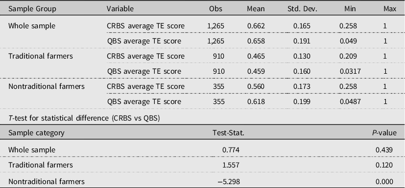
Note: CRBM refers to TE scores estimated from expenses and revenues; PBM refers to TE scores estimated from quantities of production factors and output as calculated using available price information.
The distributions of technical efficiency scores under CRS assumption are illustrated in Figure 2. Accordingly, each sample category shows a variation, but dispersedly distributed for the whole and nontraditional farms. The distribution for the traditional farms shows a normal distribution for both CRBS and QBS specifications.
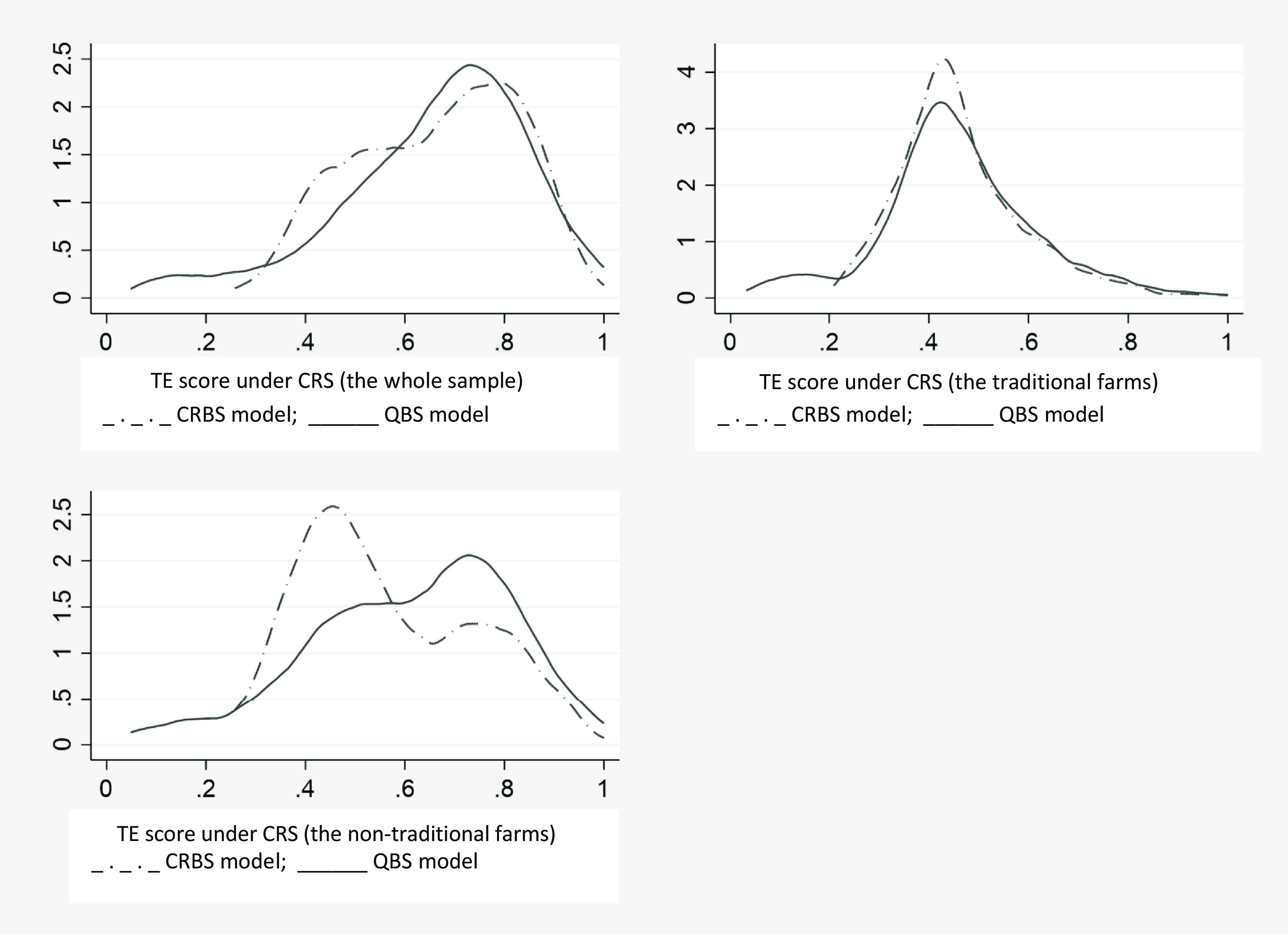
Figure 2. TE distributions for CRBS and QBS under constant return to scale assumption.
Statistical inference on VRS vs CRS assumption
Conclusions are sensitive to assumption about VRS or CRS technology; thus statistical inference on the assumptions are crucial for the continued analysis. We started the statistical inference by examining the appropriate bootstrapping technique to determine the return to scale. This allows to evade sample selection bias as the individual efficiency score is calculated with respect to the estimated frontier line rather than the actual frontier (Kneip et al, Reference Kneip, Simar and Wilson2008; Simar and Wilson, Reference Simar and Wilson1998, Reference Simar and Wilson2002). Therefore, smoothed homogenous bootstrapping technique can be used if the calculated technical efficiency scores are independent of the mix of inputs. If not, the heterogeneous bootstrapping technique should be applied. The null hypothesis is that the radial Debreu-Farrell input-based measures of technical efficiency scores are independent. Rejecting the null hypothesis favors the use of homogenous bootstrap in measuring the technical efficiency score under each technology assumption. Conversely, failing to reject the null hypothesis favors the use of the heterogeneous bootstrapping technique.
The corresponding bootstrap tests for CRS and VRS models are presented in Table 3. We run 999 bootstrap replications while computing the test statistics for each model. In all cases, the null hypothesis is rejected at 1% significance level implying the technical efficiency scores are not independent of the mix of inputs under the specified technology assumption (Table 4). Hence, rejecting the null hypothesis favors applicability of homogenous bootstrapping technique in the remaining parts of the analysis.
Once the proper bootstrapping technique is identified, selecting the correct technology assumption is crucial in DEA analysis as the corresponding efficiency score is highly sensitive to the assumption. This is observed in our estimate that there is a considerable variation in the average farmers’ technical efficiency score under VRS and CRS assumptions in both the CRBS and QBS-based estimates (Tables 2 and 3). In order to select a theoretically consistent efficiency score, a nonparametric test for the appropriate return to scale needs to be done by comparing the distributions in relation to the optimal scale points, i.e., where the CRS and VRS frontiers coincided (e.g., see Simar and Wilson, Reference Simar and Wilson2002). Accordingly, the null hypothesis that technology is globally CRS versus the alternative hypothesis that technology is globally VRS is tested. The corresponding test results reject the null hypothesis (p-value <0.000) backing the VRS technology assumption in all models. Table 5 presents returns to scale test statistics for each model.
Table 4. Tests for independence
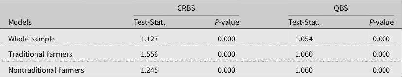
Note: CRBM refers to TE scores estimated from expenses and revenues; PBM refers to TE scores estimated from quantities of production factors and output as calculated using available price information.
Table 5. Tests for return to scale
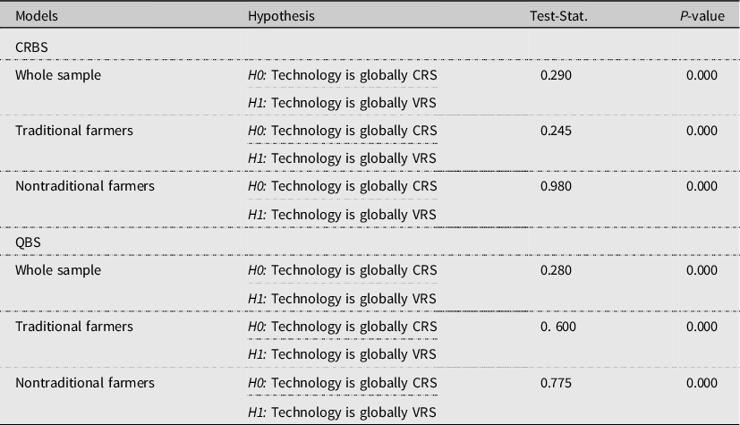
Note: CRBS refers to TE scores estimated from expenses and revenues; QBS refers to TE scores estimated from quantities of production factors and output as calculated using available price information.
Statistical inference on rankings of observations according to efficiency scores
We further tested whether there is equality in quantity and revenue and cost-based TE scores in terms of rankings of observations according to efficiency scores. Following the testing procedure by Wilcoxon (Reference Wilcoxon1945) and Wilson (Reference Wilson2003), we used the Wilcoxon signed-rank test to examine the probable equality of efficiency score from quantity and price-based models. Accordingly, the null hypothesis of equality in CRBS and QBS-based TE score is rejected (p-value <0.01) in all models (Table 6). This suggests that using aggregated data based on costs and revenues in DEA analysis can thus affect the distribution of farms from the most to the least efficient ones.
Table 6. Wilcoxon signed-rank test for quantity versus price-based TE scores
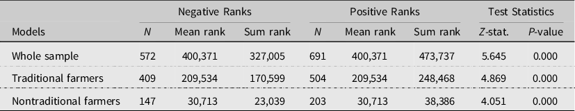
Note: CRBM refers to TE scores estimated from expenses and revenues; PBM refers to TE scores estimated from quantities of production factors and output as calculated using available price information.
Conclusions
This study investigated the role of data type in efficiency estimation and evaluated the extent to which conclusions in terms of the distribution of farms from the most efficient to the least efficient are affected if the efficiency estimation is based on quantities of inputs and outputs or on approximations of quantities using costs and revenues. By using farm-level data from Ethiopia, we found that relying on quantities of production inputs and outputs or on costs and revenues data provides different efficiency scores and significantly affects the ranking of farms in terms of efficiency. Our study introduces novel insights to the literature by being the first to highlight the possible problems with using cost and revenue data to proxy production factors and outputs in efficiency studies.
Our estimates for the whole sample based on quantities of production factors and outputs yield an average technical efficiency score of 68.4%. However, disregarding the prices and instead basing the efficiency estimates directly on expenses and revenues as proxy variables for quantities, provides an efficiency score of 72.2%. Estimates for nontraditional farmers specifically show variation in the efficiency level with an average efficiency score of 68.9% under the QBS; whereas the average efficiency score amount to 73.5% when expenses and revenues are used to proxy production factors and outputs. For traditional farms, the average efficiency scores amount to 71.7% under QBS and 67.8% when basing the efficiency scores on expenses and revenues. Statistical tests of differences in distribution from the most to the least efficient farms confirm that distributions differ in all three considered groups.
Taken together, our findings point to that relying on aggregated data could affect the distribution of farms’ efficiency scores. This has implications for subsequent analysis of, e.g., patterns of inefficiency and determinants of inefficiency, and thereby for advice and policy recommendations based on efficiency studies. This also has implications for future research in similar settings and based on similar types of data as in this study; such analysis should use price information to calculate quantities of production factors and outputs instead of using costs and revenues to proxy those quantities. While the dataset used in this study represents farming systems in Ethiopia, which are very different from those of most European countries, findings can also have implications for efficiency studies based on accounting data, which is the case for much efficiency studies based on European farming systems. For efficiency research based on accounting data, it is important to be aware of the possible bias introduced to the efficiency analysis by basing it on cost and revenue data instead of on price and quantity data. Both the possible mix between economic and technical efficiency that arises from using cost and revenue data and the possible impact of policy recommendations due to possible biased efficiency scores should be addressed. Conclusions about the direction and magnitude of the possible bias are dependent on the dataset we use; other datasets may indicate a smaller or larger magnitude. Future research will have an important role in continuing this line of research by collecting data on prices and quantities also for other types of case study farming systems; especially those where efficiency studies are generally based on accounting data. It would also be interesting in future research to pay explicit attention to what type of markets data are taken from; in particular, the extent to which markets are likely to not be competitive and to compare results across datasets representing different types of markets. In all those ways, future research would provide an important basis for discussing a possible extension of accounting-based data sources for farm-level analysis to include also price information.
Data availability statement
All the data used for this study is openly available for public use and can be accessed from the World Bank Living Standards Measurement Study (LSMS) data catalog at https://microdata.worldbank.org/index.php/catalog/lsms/?page=1&ps=15&repo=lsms The authors also indicated the data source in the reference list as: “World Bank, W. B. (2016). Ethiopia - Living Standards Measurement Study (LSMS). The World Bank Group. Available at https://microdata.worldbank.org/index.php/catalog/2783#metadata-data_access”
Financial support
This research received no specific grant from any funding agency, commercial or not-for-profit sectors.
Competing interests
Wondmagegn Tafesse Tirkaso and Helena Hansson declare none.
Appendix
Table A1. Summary of output-oriented DEA estimates by farmer category under CRS
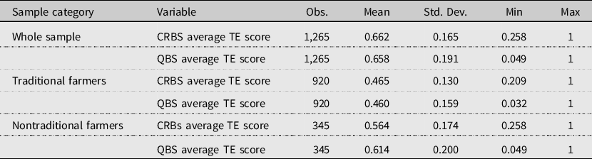
Table A2. Summary of output-oriented DEA estimates by farmer category under VRS
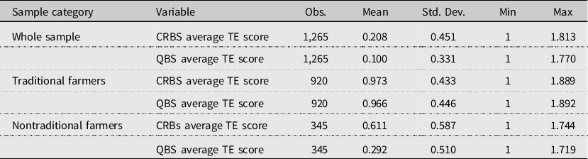
Table A3. Stochastic frontier estimates by farmer category
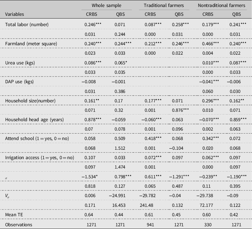
Note: Continuous variables are in logarithm. ∗∗∗ p < 0.01, ∗∗ p < 0.05, ∗ p < 0.1. The traditional farmers do not use modern fertilizers (Urea and Dap).


 Open access