


Introduction
A cow-calf producer’s calving date decision is driven by several economically relevant production outcomes. Calving date affects feed costs, calf weaning weights and marketing dates, labor availability, and, potentially, calf health. In the U.S. Southern Plains, calving typically occurs from February through April (Selk, Reference Selk2013). However, it is not uncommon that calves are born outside of this window. Earlier calving dates (January and February) allow producers to utilize labor prior to other production activities, such as cropping and haying. The tradeoffs from earlier calving include higher feed requirements, as cows’ peak nutritional demands occur when grass is either unavailable for grazing or at its lowest nutritional value (Lalman and Richards, Reference Lalman and Richards2017). Thus, early calving requires feeding of hay and protein sources, which are higher cost than grazed forages. There is also the potential for adverse weather events to negatively impact newborn calves’ health by freezing extremities (usually ears and tails but sometimes feet) and to cause hypothermia. These concerns are partially offset by higher weaning weights and early marketing dates outside of the seasonally low-price months of October and November.
Calving later (March and April) aligns cow nutritional demands with forage availability and quality. Native grasses are rapidly growing and highly nutritious in April and May, the period of greatest nutritional needs of March-April-calving cows who are in early lactation (Harty and Olson, 2020). Later born calves are less likely to experience cold weather; therefore, less likely to suffer injury or death from winter storms. However, March-April-born calves are typically marketed during seasonal low prices in October and November.
Our purpose here is to evaluate economic returns associated with alternative calving dates in the U.S. Southern Plains. Employing recent estimates of calf weaning weights from Westbrook (Reference Westbrook2019) and a series of surveys of producers, feedlot operators, and veterinarians, we model expected profits as a function of calving date. Our surveys elicited subjective producer probability estimates of frost morbidity and mortality for various calving dates as well as feedlot operators’ subjective estimates of price discounts for frost injured calves. Producers also indicated marketing dates for their current calving dates. Veterinarians contributed estimated cost differences in veterinary care due to cold weather morbidity and mortality. The profit calculation included differences in feed costs, weaning weights and marketing by calving date, and subjective estimates of calf morbidity and mortality by calving date.
Literature review
Calving season and length of calving season are known to influence profitability. Boyer et al. (Reference Boyer, Burdine, Rhinehart and Martinez2020a) show that a reduction in calving window by replacing late-calving cows improved returns when 10 or 20% of late-calving cows were replaced annually. Boyer et al. (Reference Boyer, Griffith and Pohler2020b) show that a decrease in calving window from 90 to 60 days increased per head beef cow returns by $18 ($19) for spring (fall) calving cows. Further, fall-calving cows were reported to be $38–54 per head more profitable than spring calvers. Ramsey et al. (Reference Ramsey, Doye, Ward, McGrann, Falconer and Bevers2005) found that longer calving seasons were associated with higher beef cow costs of production and lower pounds weaned per cow exposed. Payne et al. (Reference Payne, Dunn, McCuistion, Lukefahr and Delaney2009) found that fall calving was higher returning than spring calving. Stockton et al. (Reference Stockton, Adams, Wilson, Klopfenstein, Clark and Carriker2007) reported lower production costs and higher returns for June calvers in comparison to March-calvers in the Nebraska Sandhills.
Freezing temperatures are potentially detrimental to the health of younger calves. A cow in poor body condition can increase the likelihood and severity of calf cold stress (Smith Thomas, Reference Smith2018). If newborn calves do not nurse within four hours, they can experience adverse effects that are heightened in colder weather (Hall, Reference Hall2001; Smith Thomas Reference Smith2018). Olson et al. (Reference Olson, Papasian and Ritter1980) found that cold stress in calves does not substantially affect the quantity of colostrum absorbed, but the rate of absorption is greatly decreased. Newborn calves require antibodies in colostrum to protect against diseases. If they do not get sufficient and timely colostrum, the possibility of morbidity increases (Olson et al., Reference Olson, Papasian and Ritter1980). Cold-stressed calves can be more susceptible to diseases and lung problems (Jaja et al., Reference Jaja, Mushonga, Green and Muchenje2016; Olson et al., Reference Olson, Papasian and Ritter1980). A calf exposed to winter weather can also experience some challenges associated with growth (Young, Reference Young1981). When calves are kept healthy while nursing, they are healthier during later stages of the production chain (New, et al., Reference New, Ward and Zook2020). Therefore, profit varies with calving date, due to calf weaning weight and the possibility of cold weather driven morbidity.
Typically, producers calve in either the fall or spring season. In Oklahoma, spring calving is historically February through April (Selk, Reference Selk2013). An early window, January or February, carries the risk of low temperatures when calves are younger and vulnerable. Historically, Oklahoma experiences between 140 and 160 nights of freezing temperatures each year (Yu Media Group, 2020). Oklahomans can experience freezing temperatures as early as October and as late as April, with January being the coldest month (Yu Media Group, 2020). Calves born in January and February can experience snow and rain in addition to freezing temperatures (Oklahoma Climatological Survey, 2021).
Beyond the potential health of the calf, calving date also affects the alignment of the cow’s nutritional needs at different stages in her production cycle versus available forage (Funston et al., Reference Funston, Grings, Roberts and Tibbitts2016). Spring-born calves are customarily weaned in late summer or early fall (Raper and Biermacher, Reference Raper and Biermacher2016). However, calves born in January or February can be weaned and sold in mid or late summer. Oklahoma native grasses, such as little bluestem, are grazed into September (Tober and Jensen, Reference Tober and Jensen2013). By selling calves early, some producers do not take full advantage of their forage resources. Also, cow-calf producers may have to supplement cows toward the end of gestation when the nutritional needs of the cow are high, and the availability and quality of the native range is low. A 1,000-pound cow in the last third of pregnancy needs 21 pounds of dry matter intake (DMI) each day (Lalman and Richards, Reference Lalman and Richards2017). However, a 1,000-pound cow in the first 90 days postpartum needs 26–27 pounds of DMI per day (Lalman and Richards, Reference Lalman and Richards2017). These DMI values assume an unstressed cow, meaning one not experiencing heat or cold stress. A cold-stressed cow requires additional nutrients to maintain body condition. Therefore, there are economic benefits to aligning calving date with peak forage production, including reducing feed costs. On the other hand, cow-calf producers could have an advantage when selling weaned calves at seasonal high prices. For producers who sold calves in Oklahoma City over the last five years, July and December have resulted in the highest revenues (USDA Livestock & Grain Market News 2019).
The desire to sell a heavier calf by a set date may result in producers calving earlier, when the risk of bad winter weather is still high. The probability of adverse health outcomes, which can result in issues for the cow-calf producer, is considered against the monetary upside of selling heavier calves. Laudert (Reference Laudert2011) reported calves exhibiting illness received major discounts at the sale barn. Williams et al. (Reference Williams, Raper, DeVuyst, Peel and McKinney2012) quantified these discounts at $32.79 per cwt, and Mallory et al. (Reference Mallory, DeVuyst, Raper, Peel and Mourer2016) quantified them at $27.06 per cwt. The average discount for unhealthy calves based on these two studies was $29.93 per cwt. Calves with visible injuries, like frost bitten extremities, were deemed “unhealthy.” Health had the greatest influence on prices (Mallory et al., Reference Mallory, DeVuyst, Raper, Peel and Mourer2016; Williams et al., Reference Williams, Raper, DeVuyst, Peel and McKinney2012).
The impact of calving date on health and final weight is economically important to the cow-calf producer. Such problems affect the profitability of the animal for other segments of the industry as well. For example, Fulton et al. (Reference Fulton, Cook, Step, Confer, Saliki, Payton, Burge, Welsh and Blood2002) found that calves entering the feed yard healthy are more likely to have higher average daily gains than calves that enter the feed yard unhealthy (Fulton et al., Reference Fulton, Cook, Step, Confer, Saliki, Payton, Burge, Welsh and Blood2002). McNeill (Reference McNeill2001) found that sick calves gained 0.32 lb. per head per day less than healthy calves. Furthermore, the net return was almost $90 per head less for sick calves than calves that never required medical care while in the feed yard (McNeill, Reference McNeill2001). Calves that require medical care also have less desirable carcass grades (Fulton et al., Reference Fulton, Cook, Step, Confer, Saliki, Payton, Burge, Welsh and Blood2002; McNeill, Reference McNeill2001). Additionally, sick calves perform poorly at the feedlot in terms of mortality, morbidity, and rate of gain (Fulton et al., Reference Fulton, Cook, Step, Confer, Saliki, Payton, Burge, Welsh and Blood2002).
Model and survey
Three surveys were created using Qualtrics (2022), an online survey design tool, with Oklahoma beef cattle producer, veterinarian, and feedlot operator participants. The data were collected to inform the economic model and to add context to modeled results. This research was approved by Oklahoma State IRB number IRB-20-330. Data were collected from July 27, 2020 to September 30, 2020. Snowball sampling was used to obtain survey respondents. The launch of the surveys was announced in an OSU press release posted on all OSU Division of Agricultural and Natural Resources websites. This press release was also picked up by several local newspapers and other agriculture related online publications. Participation information for the surveys was featured in various OSU agricultural newsletters and email blasts. Additionally, Facebook and Twitter posts were made on OSU accounts.Footnote 1 The veterinarian survey was sent to large animal accredited veterinarians in Oklahoma through a list provided by the Oklahoma State University College of Veterinary Medicine. The feedlot survey was sent to a list of feedlots provided by the American Angus Association (American Angus Association 2020).
Each survey included a screening question to ensure respondents were completing the correct survey. If an individual indicated they were not part of the target group, they were unable to continue. For example, individuals who accessed the veterinarian survey were asked if they were a veterinarian before continuing the survey. Demographic questions such as gender, age, household income, and education were included in all surveys. Any individual who expressed they were under 18 years old were not allowed to continue past the demographics section of the survey. A test of proportions following Acock (Reference Acock2018) was completed in Stata (2021) to determine if there were statistically significant differences between the producer demographics and the U.S. Census of Agriculture (USDA-NASS 2017b). Additional calculations, such as mean responses, were calculated for all surveys. Each survey offered the opportunity for the respondent to provide additional comments at the end.
In the producer survey, researchers asked the number of years on their present farm or ranch or operating any farm or ranch, the number of years the producer owned cattle, and the number of head of cattle the producer owned. Response options were designed to match the U.S. Census of Agriculture for ease of comparison (USDA-NASS 2017a, 2017b). Respondents who did not calve heifers or cows within their operation, or who did not calve primarily in Oklahoma were prevented from continuing the survey. Producers were then asked when their calving season was and why they chose it. The survey included a series of questions related to frozen ears, tails, and legs. Questions included visual identification of frozen extremities on their own cattle, perception of frozen extremities, perception of discounts at the sale barn, and expectation of health problems in the future. Final questions included precautionary actions taken by respondents if their calves were born in colder months and cold exposure was an issue.
The veterinarian survey included questions such as where the veterinarian completed their degree, and their practice mix between small and large animal clients. It was assumed all veterinarians have an advanced degree, so they were not asked their education level. Veterinarians were asked the percentage of their business dedicated to cattle in terms of total patients or clients and the number of cattle they worked with annually. If the veterinarian indicated they did not practice on cattle, they did not continue the survey. Veterinarians that worked with cattle were asked the percentage of calves they saw with frozen ears, tails, or legs. Questions regarding the average cost of a farm visit to examine and assess the veterinary needs of an animal, and the average cost of treating a cold exposed calf including medication, treatment, or procedure was included.
Respondents of the feedlot survey were asked the capacity of their feedlot in terms of number of cattle and how many years they had been in the business. They were also asked a series of questions related to frozen ears, tails, and legs. Questions included whether frozen extremities could be seen in their feedlot, if frozen extremities were a problem, and if cattle with frozen extremities performed poorly in the feedlot. Economic considerations included: if the feedlot paid less for calves with frozen extremities, and if they avoided purchasing calves with frost damage. If discounts for cold exposure were routine, the feedlot operator provided the amount, and why a discount was given.
Cow calf producers are assumed to maximize expected profit per cow exposed by choosing calving date D, computed as in (1).
 $$\eqalign{ & \mathop {\max }\limits_D \;E[\pi |D] = \sum\limits_{i = 2}^{10} {[SteerWgh{t_i}|D \times (SteerPric{e_D}(SteerWgh{t_i}|D) - AvgDiscount|D)/2} + \cr & + HeiferWgh{t_i}|D \times (HeiferPric{e_D}(HeiferWgh{t_i}|D) - AvgDiscount|D)/2 \times (1 - retention\% ) + \cr & HeiferCullRevenue + CullCowRevenue - BullCost - FeedCos{t_i}|D - VetCost|D] \times PercentAg{e_i} \cr}$$
 $$ \textit{where} \ D\ \epsilon \left\{Jan.15,Feb.15,\textit{March}15, \textit{April}15\right\} $$
Expected annual profits are summed over cow age i from two to ten and weighted by an age distribution model taken from Bir et al. (Reference Bir, DeVuyst, Rolf and Lalman2018). Mature cows were assumed to weigh 1350 pounds at age six, growing by 4% per year until reaching mature weight (Bir et al., Reference Bir, DeVuyst, Rolf and Lalman2018).
Steer and heifer weaning weights,Footnote 2 SteerWght i and HeiferWght i , are taken from an estimation by Westbrook (Reference Westbrook2019) and vary with cow age i and calving date D. Prices for both steers and heifers, SteerPrice and HeiferPrice, are functions of weaning weights and sale dates and found using historical prices. The percentage of heifers retained was found using the age distribution model. Using results of the survey (below), expected frost damage discounts, AvgDiscount|D, vary with calving date and were subtracted from the sale price. Expected cull heifer (HeiferCullRevenue) and expected cull cow revenue (CulllCowRevenue) were calculated using the herd age distribution model and historical prices. Bull costs, feed costs, and veterinary costs are discussed below.
Expected profits were computed using GAMS (2020) for each calving date. Calving dates were taken from the producer survey. We analyzed economic returns from calving dates of January 15 to April 30 in four-week increments. A weaning weight model adapted from Westbrook (Reference Westbrook2019) was used to simulate weaning weights for steers and heifers for cows aged 2–10 years:
 $$\eqalign{ & CalfWeanWght = - 190.41 + 21.3 \times DamAge - 1.69 \times DamAg{e^2} - 16.87 \times Heifer \cr & + 98.18 \times Ln(CowWeight) + 32.6 \times ForageYield - 17.76 \times ForageYiel{d^2} \cr & + 1.92 \times AgeAtWeaning. \cr}$$
where CalfWeanWght is the weaning weight of a calf, DamAge is the dam’s age in years, Heifer = 1 for heifer calves and zero otherwise, CowWeight is the weight of the cow (cwt), and ForageYield is the amount of native forage produced each year (taken from Westbrook, Reference Westbrook2019). A calf’s age at weaning is given by AgeAtWeaning.
A mature cow weighing 1,300 pounds and a calf crop comprised of 50% steers and 50% heifers were assumed (Bir et al., Reference Bir, DeVuyst, Rolf and Lalman2018). LMIC (2020), and data were used to determine prices for feeder steers and heifers. Using Raper (Reference Raper2020b), we assumed weaning ages were 9.04 months for January-born calves, 7.80 months for February-born calves, 7.70 months for March-born calves, and 7.50 months for April-born calves. Weaning age was then used to determine sale date assuming no preconditioning. Weaning percentage per cow exposed was 89.8% (Raper, Reference Raper2020a). Calf revenue was determined based on the weight of the calf and the sale price for each year, cow age, sex of the calf, calving date, and weaning percentage. Expected discounts for frost exposure were included based on producer and feedlot operator surveys. A heifer retention rate of 20% was assumed (Bir et al., Reference Bir, DeVuyst, Rolf and Lalman2018). Cull heifer revenue was approximated using LMIC data (2020). Cull heifers were assumed to be sold as feeder heifersFootnote 3 weighing 845 pounds (Bir et al., Reference Bir, DeVuyst, Rolf and Lalman2018).
A herd distribution from Bir et al. (Reference Bir, DeVuyst, Rolf and Lalman2018) and a cull rate at each age from DeVuyst et al., (Reference DeVuyst, Munson, Brorsen, Lalman, Hannah, Swanson and Ringwall2021) were used with the weaning weight equation to create a distribution of weaning weights and cull cow weights. Cull cow price was taken from LMIC (2020). Cull cow revenue was determined given cow weight, cull price, cull rate, and herd percentage for each year, cow age, and calving date. The Producer Price Index (U.S. Bureau of Labor Statistics, 2021) was used to convert historical prices to 2020 values. Total revenue was equal to the sum of calf revenue, cull cow revenue, and cull heifer revenue.
Expected feed costs of a cow-calf operation at calving date are given as
 $$\eqalign{FeedCos{t_i}|Date =\, & E\boldsymbol( {Cube{s_i}\; \times \;CubePric{e_t} + Ha{y_{it}}\; \times \;1.20\; \times \;HayPric{e_t}} \cr & {+ {{Forag{e_{it}}} \over {ForageYield}}\; \times {1 \over {0.25}}\; \times \;Rental\;Rate} \boldsymbol)}$$
where the feed cost is the cost of feed for cow-age i in year t with respect to calving date, Cubes it expresses the quantity of cubes for pair i in year t, CubePrice t is the price of cubes in year t, and Hay it is the quantity of hay required given pair i and year t assuming 20% hay loss (DeVuyst et al., Reference DeVuyst, Munson, Brorsen, Lalman, Hannah, Swanson and Ringwall2021), HayPrice t expresses the price of hay in year t, Forage it is the quantity of forage (pounds) required for pair i in year t, ForageYield is forage yield (pounds per acre), 25% is the assumed forage utilization rate (DeVuyst et al., Reference DeVuyst, Munson, Brorsen, Lalman, Hannah, Swanson and Ringwall2021), and RentalRate expresses the cost of renting land.
USDA data were used for the price of hay (USDA-NASS 2020a), wheat (USDA-NASS 2020b), cottonseed (USDA-AMS, 2021), and corn (USDA-NASS 2020c). USDA data were also used for forage yield in Payne County (USDA-NASS 2020d), and rental rate assuming cash rent on pastureland (USDA-NASS 2021). Molasses pricesFootnote 4 were taken from USDA-ERS (2020). A 20% protein cube was assumed with 65% wheat midds, 30% cottonseed, and 3% molasses (Bir et al., Reference Bir, DeVuyst, Rolf and Lalman2018).
Rations were developed using CowCulator (Lalman et al., Reference Lalman, Gross and Beck2020), generating annual forage, hay, and cube requirements. Rations varied for January-, February-, March-, and April- calving herds. It was assumed grazing was not available in December, January, and February, so hay was the only source of forage in the rations in those months. The 1.20 hay loss factor assumed a round bale with a rack (Angus Beef Bulletin 2012). Forage cost was determined by the number of acres required based on year, age of the cow, and calving date multiplied by the rental rate. Feed cost was determined given cube cost, hay cost, and forage cost for each year, cow age, and calving date. Annual veterinary expense was assumed at $25 per cow, and an annual bull cost of $50 per cow (Munson et al., Reference Munson, DeVuyst, Brorsen and Lalman2022). Fixed costs were ignored as they do not change with the calving date.
The percentage of frost-damage calves reported by producers was calculated using producer responses. Answer choices “0–10” and “11–20” for each month were analyzed. We assumed most producers were indicating on the lower side of both bounds based on the distribution of answers. Therefore, the data used in the analysis were skewed leftFootnote 5 to 2.5% and 12.5%. The average cost for a veterinary call was approximately $70, and $5.70 for medication per the veterinarian survey. Almost half (48%) of producers do not seek veterinary assistance with frost-related issues. We assumed producers not seeking frost-related veterinary care were those experiencing 2.5% calf crop frost exposure; and those needing veterinary assistance (52%) were experiencing 12.5% calf crop frost exposure. Therefore, the veterinary costs were multiplied by the probability that a producer saw frost damage in their cattle as indicated in the producer survey with respect to each calving month. The cost of a veterinary call and medication costs were added together. The probabilities of producers who saw frost damage in their cattle were weighted by calving month based on answer choices indicated in the producer survey. Veterinary costs were multiplied by the frequency of frost injured calves for each month assuming again that producers who selected “11–20” were the ones requesting veterinary assistance. An expected veterinary cost per cow for each of the four calving months was then determined.
Researchers calculated expected damages for each calving month using the producer’s anticipated discount rate and the feedlot operators’ anticipated discount rate. Expected cow-calf producer damages and expected feedlot damages were both determined based on their respective perceived risk of a sale barn discount, the amount of the discount, percent of frost damage seen, and the percent of producers who saw frost damage for each calving month. The annualized returns per head to the producers using both the feedlot operators’ and producers’ anticipated discount rates were calculated and compared.
We also assessed the sensitivity of our results to changes in the frequency of frost damage and protein cost. We compare the qualitative conclusions between the baseline model evaluation and those from the sensitivity analysis.
Results
Survey results
Of the 205 respondents who accessed the producer survey, 175 completed every question. Ninety-seven percent of producers said most of their bred cows and heifers were located primarily in Oklahoma during their calving seasonFootnote 6 (n = 205). Seven hundred twenty-one veterinarians were contacted via the list provided by the Oklahoma State University College of Veterinary Medicine. Of those, 20 individuals were unreachable or indicated they were not large animal veterinarians. Ninety-eight people accessed the veterinarian survey and 68 completed every question.Footnote 7 The feedlot list from the American Angus Association provided 21 contacts. Six feedlots could not be contacted. Seven feedlot operators accessed the feedlot survey with six completing it. Responses to surveys are summarized in Table 1. Size of operations results are summarized in Table 2.
Table 1. Cattle producers, large animal veterinarians, and feedlot operators, reported demographics

* USDA-NASS, 2017.
Table 2. Size of operation for cattle producers, large animal veterinarians, and feedlot operators. Percentage of total respondents

Respondents to the producer survey were primarily from Payne, Noble, and Kay counties in Oklahoma (8, 8, 5%, respectively n = 205). A high number of Payne County respondents was expected as Oklahoma State University is in Payne County. Of the veterinarians who completed the survey, 83% received their veterinarian degree from Oklahoma State University. This was also expected, as the contact list was obtained from the Oklahoma State University College of Veterinary Medicine and restricted to those actively practicing in Oklahoma.
Producers report calving mostly in March (81%), April (59%), and February (55%) (n = 185, multiple selections allowed). January-calving producers (23%) stated it was driven by marketing strategy (58%), grazing management strategy (45%), and experience (28%). Producers who calved in February, March, and April ranked grazing management strategy first (58, 57, 56%, respectively), marketing strategy second (55, 54, 44%, respectively), and convenience third (29, 29, 33%, respectively).
Thirty-eight percent of veterinarians said they defined their practice as large animal, while 49% selected mixed practice (n = 84). Only 13% indicated their practice was small animalFootnote 8 . Forty-six percent indicated cattle made up of less than half of their practice in terms of total patients or clients and 43% answered cattle made up more than half of their practice in terms of total patients or clients.
When asked about producers’ experience with cold exposure, 97% selected they saw “0-10%” of their calf crop with frozen ears, tail, and legs. Of the 174 producers who were asked what they did if they saw cold exposure in their calves, 15% reported they retained ownership until the calf reached a heavier weight, and 1% obtained a certificate from their veterinarian ensuring future buyers their calves were healthy. Seventy-four percent said they did not see problems with cold exposure. Of the veterinarians who worked with cattle (n = 67), 73% saw frozen ears, tails, and legs on 0–2% of the calves they worked with and 21% saw frozen ears, tails, and legs on 3–5% of calves. Ten percent of the veterinarians who worked with 501–1,000 cattle saw frost exposure in 0%-2% of calves. Nine percent of the veterinarians who worked with 101–250, 5,001–10,000, and 10,001–25,000 cattle saw frost exposure in 0–2% of calves. One percent of the veterinarians who worked with 501–1,000 cattle saw frost exposure in 12–20% of calves.
Producers (n = 186) and feedlot operators (n = 6) were ambivalent on whether frozen ears, tails, and legs are an economic problem. On a 1–5 scale with “1” equating to disagreeing that frozen appendages are a problem they experience and “5” equating to strong agreement, producers had a mean score of 2.6, while feedlot operators had a mean score of 3.2. However, producers view the possibility of discounts at the sale barn as a greater danger than feedlot operators do. Regarding discounts at the sale barn due to frost exposure, producers had a mean of 3.6. For the statement, would they pay less for cattle with frost exposure, feedlot operators had a mean score of 2.8. Producers and feedlot operators had similar opinions about whether frost exposure would lead to potential health problems in the future; producers had a mean of 3.1, while feedlot operators had a mean of 3.0. For expectation that cattle with frost exposure would perform poorly in the feedlot compared to their counterparts, feedlot operators had a mean score of 2.7. For the statement they avoided purchasing calves with freeze damage, feedlot operators had a mean of 2.8.
Twenty-five percent of all producers (n = 186) expect to receive no discount at the sale barn for frozen ears, tails, and legs, 19% expect to receive a $0.01–$1.00/cwt discount, and 18% expect to receive a $1.01–$5.00/cwt discount. Feedlot operators’ opinions (n = 6) varied on the discount producers can expect to receive for cold exposure. Feedlot owners acknowledged their reasons for discounting as: decreased performance, poor gains or lower feed conversion, and mobility problems (20% for each).
Economic model results
Total revenue was highest for the calving week of January 15 and lowest for the calving week of April 30 (Table 3). This result is driven by weaning age and weight. Survey respondents reported weaning/selling calves at 276 days, on average, with January calving. That is more than 30 days older than the other four calving dates, resulting in heavier calves and higher calf revenue. Note, the weaning weight model (equation 2) shows calves gaining 1.92 pounds per day while nursing. So, January-born calves weigh 67 pounds more than the February-born calves. The revenues from the other four calving dates are within $20 per head of each other, driven by the combination of weaning weight and market prices.
Table 3. Economic results ($/head) by calving date
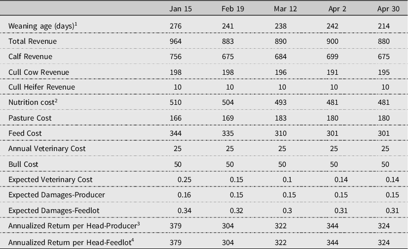
1 Average weaning age from survey results.
2 Nutrition costs are derived from rations calculated using Cowculator (Lalman et al., Reference Lalman, Gross and Beck2020).
3 Utilizes cow-calf producer estimates of frost damage frequency and market discounts.
4 Utilizes cow-calf producer estimates of frost damage frequency and feedlot operator estimates of market discounts.
Calf revenue must then be compared to production costs. Feed costs are the largest component of production expense. Early- calving cows, as expected, have higher feed costs. Since nutritional demands do not line up with grass production, January and February-calving cows are fed hay and supplements during higher demand. This leads to higher feed costs compared to other calving dates. As a result, January calvers cost almost $30 per head more to feed than April calvers.
As one of the goals of the survey and analysis is to consider the impact of freezing temperatures on calf health, veterinary costs, and revenues, approximations of these impacts were included in the budgets. Few of the respondents expressed concern with frost-related impacts. Between the five calving dates, the expected costs and losses from frost damages range from $0.25 to $0.41 per head based on cow-calf producer survey responses. Thus, these damages have no significant impact on calf returns. The impact on sale price was also negligible with no significant differences between sellers (cow-calf operators) and buyers (feedlot operators).
Annualized returns per head using the producers’ and feedlot operators’ anticipated discount rates were both highest for January-calving herds and lowest for the calving week of mid-February (Table 3). There was a $65 difference in annualized return per head between the two dates. The driving factor was calf age at weaning and sale.
The USDA Animal and Plant Health Inspection Service (APHIS) performed a survey in 2017 about cow-calf management practices in the United States and found similar results to this producer survey. In their survey, Oklahoma was included in the west region. They found 31.9% of the producers in their survey calved in January, 48.6% calved in February, 64.6% calved in March, and 59.1% calved in April (USDA-APHIS, 2020). Researchers also found March to be the most popular calving month, with April and February at second and third, respectively. The calving percentage for the west region was 80.2% for heifers, and 92.6% for cows (USDA-APHIS, 2020). The heifer calving percentage found by APHIS (2017) was significantly lower than the percentage researchers used in this analysis (89.8%). However, the cow calving percentage used was similar.
Conclusions
In the USDA-APHIS (2020) survey, the most common reasoning behind calving date was tradition. The second most common answer was weather, and the third most common answer was grazing management strategy. In this producer survey, tradition was the third most common answer for January producers, and the fifth most common answer for February, March, and April producers. However, grazing management strategy was the second most common answer for January producers, and the most common answer for February, March, and April producers. In this producer survey, marketing strategy was the most common answer for January producers and the second most common answer for February, March, and April producers. Marketing strategy was the fourth most common answer in the USDA-APHIS (2020) survey. The categorization of the USDA-APHIS survey at the regional level, not at the individual state level, could drive the differences in results. Additionally, using the snowball survey collection method, researchers found some statistical differences between the results found and the U.S. Census of Agriculture.
The model computed annualized returns per head for five calving dates (in four-week intervals), using producer and feedlot operator perceptions of frost discounts. Feed costs varied by calving date. The age, and thus, weight of calves varied by calving date based on producer survey responses. January-calving producers held calves longer, resulting in heavier sale weights and higher revenues. These higher revenues more than offset higher feed costs for the January-calving herds. As was noted, producers did not report significant costs associated with frost damage from early calving. In net, January-calving herds had the highest annualized net returns, a result driven by heavier weaning weights.
Early-April-calving herds had the second highest returns. Calf age at weaning, and thus weight, was the second highest, but only one day older than February-born calves. However, feed costs were tied for the lowest. The resulting net return per head was $35 lower than January-calving herds and $20 higher than late- April-calving herds. Mid-February-calving herds were budgeted to have the lowest net returns. Feed cost was the second highest, and revenue was the second lowest. So, net returns were $75 lower than January and $40 per head lower than early April.
However, survey results show March and April were the most common calving months. This may be due to weather, feed costs, and labor demand concerns. If calves were weaned at a consistent age of 205 days, January lost its advantage and became the least profitable. In this case, the April-calving dates were the most profitable.
One potential weakness with our analysis is conception rate. Heifers and cows bred in July and August might have lower conception rates due to lower bull fertility in hotter months (see, e.g., Morrell, Reference Morrell2020). Cows calving in April rebreed in July–August when bull fertility is reduced. So, our results are potentially biased. Since little is published on beef cow conception rates by calendar month in the US Southern Plains, we are unable to directly model potentially lower conception rates differences. So, we calculate the percentage difference in conception rates to make producers indifferent between an early-April calving date and a mid-February calving date. If conception rates are 3.5% lower for April calvers than for February calvers, returns are equal.
Data availability statement
Data is available upon request.
Author contribution
A.U., C.B., and E.D.; Methodology, A.U., C.B., and E.D.; formal analysis, A.U., C.B., and E.D.; data curation, A.U., C.B., and E.D.; writing—original draft, A.U., C.B., and E.D., writing—review and editing, C.B., and E.D.; supervision, C.B., and E.D.; funding acquisition, C.B., and E.D.
Financial support
This research was supported by the USDA-NIFA Hatch Multistate Project NC-1177. Partial funding provided by the Rainbolt Chair of Agricultural Finance, Oklahoma State University.
Competing interests
The authors do not declare any competing interests.


 Open access