


Introduction
Sustained productivity growth in US agriculture is crucial to ensure competitiveness in the world market. US farm output has grown remarkably since the 1950s – by more than two-fold and this historic rise was mainly driven by productivity growth (USDA ERS, 2021). Efforts to develop and disseminate new technologies can be traced back to public research and development (R&D) activities conducted in universities and government institutions. To ensure long-term farm productivity growth, continued investments in public agricultural R&D are needed. The economic gains from R&D-driven productivity growth are well researched (Alston et al., Reference Alston, Andersen, James and Pardey2011; Andersen and Song, Reference Andersen and Song2013; Fuglie, Reference Fuglie2017; Jin and Huffman, Reference Jin and Huffman2016; Plastina and Fulginiti, 2011; Wang et al., Reference Wang, Plastina, Fulginiti and Ball2017). In a recent meta-analysis of 492 studies, Rao et al. (Reference Rao, Hurley and Pardey2019) estimated that the median internal rate of return from agricultural R&D is around 34.0% per year for developed countries. Similarly, the meta-analysis of Alston et al. (Reference Alston, Pardey and Rao2022) found that past investments in international agricultural research for developing regions indicate benefit-cost ratios at around 10:1.
However, there has been a slowdown in investments in the US public agricultural R&D systems (Fuglie et al., Reference Fuglie, Clancy, Heisey and Macdonald2017; Nelson and Fuglie, Reference Nelson and Fuglie2022). The stagnation of public funding for US agricultural scientific research is alarming when contrasted with the growth in R&D investments in middle-income countries, particularly in China which has surpassed US research spending in recent years (Clancy, Fuglie, and Heisey, Reference Clancy, Fuglie and Heisey2016; Pardey et al., Reference Pardey, Alston, Chan-Kang, Hurley, Andrade, Dehmer, Rao, Kalaitzandonakes, Carayannis, Grigoroudis and Rozakis2018). Less R&D spending at home and greater investments abroad could erode the competitiveness of US farm exports in the coming decades.
In addition to the economic benefits, agricultural productivity growth from R&D investments can also offer GHG mitigation co-benefits. Several studies which use global models of the agricultural sector – models which explicitly incorporate drivers of agricultural demand and supply, farm input use, and agricultural trade – have shown that greater agricultural productivity could dampen future agricultural land expansion and farm greenhouse gas (GHG) emissions. Valin et al. (Reference Valin, Havlík, Mosnier, Herrero, Schmid and Obersteiner2013) examined the global GHG emissions impacts of productivity growth in several crop and livestock sectors as well as other land-based sectors. The authors focused on methane emissions from paddy rice and livestock, emissions from fertilizer use, as well as land-use change emissions. They found that under business as usual, world agricultural GHG emissions are expected to increase by around 30% between 2000 and 2050, from 3.5 to 4.6 gigatons (Gt) carbon dioxide-equivalent per year (CO2-eq/year). The authors also found that greater productivity through higher yield growth and yield convergence across crops and livestock sectors could reduce global farm GHG emissions by roughly 10% relative to the 2050 baseline. Jones and Sands (Reference Jones and Sands2013) estimated that without total factor productivity growth in crop and livestock production, global farm GHG emissions would rise by 47% between 2004 and 2034. WRI (2019) used a global agricultural model to calculate future changes in agricultural production, land use, and greenhouse gas emissions between 2010 and 2050. The authors estimated several scenarios using different assumptions regarding future diets, food waste mitigation, productivity growth, and emission reduction in agriculture. Under business as usual, the authors estimated that GHG emissions from global agricultural production and land-use change are expected to increase by around 25% between 2010 and 2050, from 12 to 15 Gt CO2-eq/year. If productivity remains flat over this period, future emissions are projected to rise to 33 Gt CO2-eq/year, primarily due to increased emissions from land-use change.
This study formally links the literature on R&D-driven productivity growth to previous work on the GHG mitigation benefits from increased productivity growth. By connecting agricultural productivity directly to R&D spending, it is possible to calculate the economic costs and benefits of productivity-based GHG mitigation strategies. Specifically, this study examines the economic and GHG mitigation benefits from increased public agricultural R&D investments in the US over 2025–2035. This study focuses on US agriculture and directly calculates the implied growth in agricultural productivity from US R&D spending using statistically estimated parameters from a historical analysis of the gains from US public R&D spending (Baldos et al., Reference Baldos, Viens, Hertel and Fuglie2018). It also uses technological spillover estimates from the literature (Fuglie, Reference Fuglie2017). These productivity changes are then used in a global economic model of agriculture to see how future increases in US R&D investments change the trajectories of agricultural production, land use, and GHG emissions at the global level and in the US. A farm input reduction scenario is also estimated to show how policies directly mitigating land use and GHG emissions in US agriculture affect production and price outcomes.
The results show that over the period 2017 to 2050, greater public R&D investments in US agriculture could significantly boost crop and livestock production, limit agricultural land expansion and GHG emissions, and reduce food prices globally. However, the reduction in US farm input use and associated GHG emissions from R&D is dampened by increased price competitiveness of US agricultural commodities in the world market and resulting expansion in US production. Reducing farm input use alone can drastically reduce US agricultural GHG emissions, but at the cost of lower farm output and higher commodity prices. Substantial reductions in US GHG emissions and greater agricultural production can only be achieved when both R&D investment and farm input constraint policies are implemented.
Models and methods
Modeling R&D investments and knowledge stock accumulation
The empirical literature on the linkages between the flow of R&D spending, the stock of accumulated knowledge capital, and subsequent productivity growth is well established (Alston et al., Reference Alston, Andersen, James and Pardey2011; Griliches, Reference Griliches1979; Heisey, Wang, and Fuglie, Reference Heisey, Wang and Fuglie2011; Huffman, Reference Huffman2009). The framework involves two main stages. In the first stage, knowledge capital stocks are constructed from the stream of R&D spending using R&D lag weights. Knowledge capital consists of the technological and human capital needed to develop and propagate high-yielding crop varieties as well as modern farm management techniques and machineries. Initially, the R&D spending contributes little to knowledge capital accumulation, but its effect builds over time as technology arising from that research matures and is eventually disseminated to farmers. Eventually, the effects peak when technology is fully disseminated, and then wane due to technology obsolescence. In the second stage, after converting the R&D spending flows to knowledge capital stocks, the growth in stocks is then linked to growth in agricultural total factor productivity (TFP) growth via elasticities which describe the percent rise in TFP given a 1 percent rise in knowledge capital stock. TFP growth is a measure of productivity which accounts for growth in total output given growth in overall input use, including land, labor, capital, and intermediate inputs such as fertilizer.
The functional form and length of the R&D lag weights have been extensively examined by Alston et al. (Reference Alston, James, Andersen and Pardey2010). The authors estimated the productivity returns in R&D investments and extension spending using US state-level data. The authors calculated knowledge stocks using the 50-year gamma distribution which is their base case. The authors argued that imposing shorter lag length could result in overstating the impacts of R&D spending. They also explored different lag lengths (20 and 35 years) and compared the results with the trapezoidal distribution – the recommended distribution based on the previous studies. The authors then estimated returns to R&D and extension by estimating the elasticity of multifactor productivity to knowledge stocks using both linear and log model specifications. The authors found that the elasticities estimated under the gamma distribution are less sensitive to longer lag lengths. It also results in smaller errors when predicting changes in multifactor productivity under the log model specification.
Baldos et al. (Reference Baldos, Viens, Hertel and Fuglie2018) examined the historical gains in national US R&D spending using Bayesian econometrics. The authors compiled annual public agricultural R&D expenditures (in billion 2005 USD) from spending data by USDA intramural research agencies in particular the Agricultural Research Service and the Economic Research Service, State Agricultural Experiment Stations, and Schools of Veterinary Medicine. Following Alston et al. (Reference Alston, James, Andersen and Pardey2010), the authors used the gamma structure with a 50-year lag span when calibrating the R&D lag weights. However, unlike previous studies, the authors estimated the parameters of the gamma distribution under different model specifications of the impact of R&D stocks to TFP. The results of the study suggest that the estimated parameters governing the gamma distribution are around δ = 0.74 and λ = 0.86 with the estimated TFP R&D stock elasticity at around α = 0.34 (i.e. a 0.34 percent rise in TFP given a 1 percent rise in knowledge capital stock).
This study borrows heavily from the data and parameter estimates from Baldos et al. (Reference Baldos, Viens, Hertel and Fuglie2018). Equation 1.a shows the R&D lag weight (β RD, i ) in year i gamma distribution given lag length L = 50 and gamma distribution parameters δ and λ for each time period. Equation 1.b requires that the sum of the lag weights is equal to 1. Once computed, R&D knowledge stocks (RD US, i ) are computed by multiplying the R&D lag weight (β RD, i ) and R&D spending (XD US, i ) in year i (Equation 2). Equation 3 defines the year-on-year percent changes in TFP (Δ%TFP US, i ) which are calculated from the annual percent changes in R&D stocks (Δ%RD US, i ) using the TFP R&D stock elasticity (α US )
 $$ \beta _{RD,i}=\left(i+1\right)^{{\delta \over 1-\delta }}\left(\lambda \right)^{i}/\sum _{i=0}^{L}\left(i+1\right)^{{\delta \over 1-\delta }}\lambda ^{i} $$
 $$ \sum _{i=0}^{L}\beta _{RD,i}=1 $$
 $$ RD_{US,i}=\sum _{i=0}^{L}\beta _{RD,i}XD_{US,i} $$
 $$ \Delta \% TFP_{US,i}=\alpha _{US}\Delta \% RD_{US,i} $$
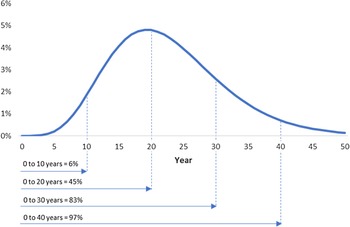
Figure 1 shows the distribution of R&D knowledge stocks from R&D investments given the parameters of the lag weights adopted in this study. Note that the R&D lag weights are used to capture the temporal dynamics of technological development, adoption, and obsolescence from public agricultural R&D spending. After a decade from the initial expenditure (Year 0 to Year 10), only 6% of the R&D spending is converted into knowledge capital. After 20 years (Year 0 to Year 20), roughly 45% of the R&D spending in the initial period is transformed to knowledge capital. This suggests that, although some types of R&D such as highly applied research may have near-term benefits, in the near term, R&D spending generally provides minimal gains and that the gains from these investments should be evaluated for several decades.

Figure 1. Distribution of R&D knowledge stock from R&D investments over a 50-year period.
R&D investments in the US also result in technical improvements which are transmitted to the rest of the world. To explore the impact of technological spillovers to the rest of the world from US R&D investments, the methods and parameters from Fuglie (Reference Fuglie2017) are used. The author reviewed the literature on the estimated R&D stock TFP elasticities as well as R&D spillover elasticities for key regions. The author also calculated the international R&D stocks – which generate R&D spillovers – from the R&D spending in the developed world. Since the full data used by Fuglie (Reference Fuglie2017) is not publicly available, side calculations are necessary to calculate the international R&D stocks from the available US data. Shares of R&D stocks for US (θ US, 2011 = 0.335) and other key regions in the developed world (1 − θ US, 2011) from Fuglie (Reference Fuglie2017) are combined with the estimated US R&D knowledge capital stocks (RD US, 2011) in this study to calculate total international R&D stocks (RD INTL, 2011) in year 2011 (Equation 4). This study assumes that future contributions of R&D stocks from non-US regions are fixed (i.e. international R&D stocks are mainly driven by R&D stocks from the US) (Equation 5). Regions which historically benefited from R&D spillovers include Western Europe, Oceania + South Asia, Developed Asia and Latin America. Actual agricultural TFP data for these regions (j) for year 2011 are taken from USDA ERS (2021) and are projected to 2050 using the year-on-year change in international R&D stocks (Δ%RD INTL, i ) and R&D spillover TFP elasticities (α j ) from Fuglie (Reference Fuglie2017) (Equation 6). These regional elasticities are based on country and regional estimates in the literature. Specifically, the TFP R&D elasticities are 0.24, 0.12, and 0.36 for Western Europe, Oceania + South Africa, and Latin America, respectively. Due to lack of regional data, the average elasticity for the Develop Regions (0.21) is applied to Developed Asia.
 $$ RD_{INTL,2011}=RD_{US,2011}{1-\theta _{US,2011} \over \theta _{US,2011}} $$
 $$ RD_{INTL,i}=RD_{US,i}+RD_{INTL,2011} $$
 $$ \Delta \% TFP_{j,i}=\alpha _{j}\Delta \% RD_{INTL,i} $$
Projecting global agriculture using the SIMPLE Model
To quantify economic and environmental impacts from increased US R&D spending, the SIMPLE model is used (a Simplified International Model of agricultural Prices, Land use, and the Environment) (Appendix 1). As the name suggests, SIMPLE focuses on the key drivers and economic responses which govern long-run developments in the farm and food system (U.L.C. Baldos and Hertel, Reference Baldos and Hertel2013). In the model, per capita food demands are driven by exogenous per capita income growth and respond to endogenous changes in food prices with these responses varying by income level. Consumers in wealthy regions are less responsive to price and income changes than those residing in low-income regions. Aggregated food commodities in SIMPLE include crops, livestock products, and processed foods. Consumption patterns evolve to reflect observed shifts in dietary preferences – moving away from crops towards livestock and processed foods as incomes rise.
Regional production systems in SIMPLE are modeled using a constant elasticity of substitution production framework. Crops are produced by combining land and an aggregate noncropland input, with the latter input representing all other factors of production used by the crop sector, including fertilizer, labor, and machinery, among other farm inputs. Crop outputs are demanded in four uses, namely: direct food consumption, feed use in the livestock sectors, raw input use in the processed food industries, as well as feedstocks in the biofuel sector in each region. The capacity for input substitution between land and noncropland inputs makes it possible to endogenously increase crop yields. Livestock and processed food sectors use crop and non-crop inputs. Crop outputs are traded within regions and in the international market. The standard model assumes that livestock and processed foods are traded only within a region, but in this study the model is modified to incorporate international trade for these commodities. Specifically, local and global markets for these commodities are defined using value of consumer purchases and producer supply from GTAP V.10 (Aguiar et al., Reference Aguiar, Chepeliev, Corong, McDougall and van der Mensbrugghe2019). Demand and supply equations for livestock and processed foods in the local and global market are added to the model as well as additional local and global market clearing equations (see Appendix 1). This allows consumers and producers of these products to purchase in the local and global markets. The evolution of the global farm system is also driven by exogenous productivity trend effects owing to endogenous productivity responses to past and future investments in agricultural R&D.
Appendix 1 shows the mathematical description of SIMPLE. In the model, exogenous productivity growth from greater R&D spending is modeled using the input neutral productivity parameter in the crop sector and in the livestock sector (ao (Crops,g), ao (Lvstck,g)). Greater productivity growth has the direct effect of reducing the derived demand for inputs in these sectors (see derived demand equations in Appendix 1) which leads to lower input use. However, greater productivity growth also has the direct effect on boosting the per unit revenue for these commodities (p S(Crops,g) + ao (Crops,g), p S(Lvstck,g) + ao (Lvstck,g)) which encourages greater production (see zero profit equations in Appendix 1).
In this study, the SIMPLE model is also modified to report changes in agricultural GHG emissions, specifically emissions from crop and livestock production as well as land-use change emissions due to cropland expansion. Country-level data on GHG emissions from agricultural production are based on the GTAP v.10 standard database (Aguiar et al., Reference Aguiar, Chepeliev, Corong, McDougall and van der Mensbrugghe2019) which reports CO2 emissions from fossil fuel combustion using detailed energy volume data from the International Energy Agency (IEA, 2016) and combustion factors from the Revised, 1996 IPCC Guidelines for National Greenhouse Gas Inventories (IPCC/OECD/IEA, 1997). These emissions are aggregated to the SIMPLE regions and are linked to changes in non-feed inputs and non-land inputs. GHG emissions from methane, nitrous oxide, and fluorinated gases are based on the non-CO2 GTAP database (Chepeliev, Reference Chepeliev2020) which use FAO data (2020) for agricultural emissions for both inputs and outputs. These input and output emissions are linked to changes in crop and livestock outputs and inputs in SIMPLE. Land-use change emissions from converting natural land into cropland rely on the global carbon stocks calculated by West et al. (Reference West, Gibbs, Monfreda, Wagner, Barford, Carpenter and Foley2010). These carbon stocks are constructed using spatially explicit datasets on potential vegetation and soil carbon and are linked to regional changes in cropland area.
Experimental design for future projections
Projections for the period 2017 to 2050 using the SIMPLE model require future growth rates in population, income, biofuel demand, and total factor productivity in the crops, livestock, and processed food sectors. In this study, sources of these future growth rates are as follows (Table 1). The population and income growth rates are based on the Shared Socio-economic Pathways (SSP) Database v.2 (Gidden et al., Reference Gidden, Riahi, Smith, Fujimori, Luderer, Kriegler and Takahashi2019; Riahi et al., Reference Riahi, van Vuuren, Kriegler, Edmonds, O’Neill, Fujimori and Tavoni2017; Rogelj et al., Reference Rogelj, Popp, Calvin, Luderer, Emmerling, Gernaat, Fujimori, Strefler, Hasegawa, Marangoni, Krey, Kriegler, Riahi, van Vuuren, Doelman, Drouet, Edmonds, Fricko, Harmsen, Havlík, Humpenöder, Stehfest and Tavoni2018). The SSPs are a range of pathways, developed for use in climate modeling, that describe alternative trends in global socio-economic development. In this study, SSP2 is used, a “middle of the road” scenario in which historical patterns of development continue, income growth proceeds unevenly, and global population growth is moderate (Riahi et al., Reference Riahi, van Vuuren, Kriegler, Edmonds, O’Neill, Fujimori and Tavoni2017). In addition to population and income, future food demand will also be affected by crop feedstock demand for biofuel production. Projections of regional biofuel consumption are based on the “Current policies” scenario published in the World Energy Outlook (IEA, 2019), which serves as a business-as-usual-scenario. In this study, regional TFP growth rates for the crops and livestock sectors are based on adjusted historical estimates from Fuglie (Reference Fuglie and Fuglie2012) and projections from Ludena et al. (Reference Ludena, Hertel, Preckel, Foster and Nin2007), respectively. Lacking detailed TFP projections for the processed food sector, historical rates from Griffith et al. (Reference Griffith, Redding and Reenen2004) are used, assuming that these rates apply in the future and across all regions. These growth rates are used to generate the “S1 Baseline” which is the business-as-usual-scenario. The baseline scenario also assumes real US R&D spending increases by 1.9% per year, the average annual growth rate from 1971 to 2010 (Baldos et al., Reference Baldos, Viens, Hertel and Fuglie2018).
Table 1. Summary of scenarios

1 Shared Socio-economic Pathways (SSP) Database v.2 (Gidden et al., Reference Gidden, Riahi, Smith, Fujimori, Luderer, Kriegler and Takahashi2019; Riahi et al., Reference Riahi, van Vuuren, Kriegler, Edmonds, O’Neill, Fujimori and Tavoni2017; Rogelj et al., Reference Rogelj, Popp, Calvin, Luderer, Emmerling, Gernaat, Fujimori, Strefler, Hasegawa, Marangoni, Krey, Kriegler, Riahi, van Vuuren, Doelman, Drouet, Edmonds, Fricko, Harmsen, Havlík, Humpenöder, Stehfest and Tavoni2018).
2 World Energy Outlook (IEA, 2019).
3 Crop, livestock, and processed food TFP growth taken from Fuglie (Reference Fuglie and Fuglie2012), Ludena et al. (Reference Ludena, Hertel, Preckel, Foster and Nin2007), and Griffith et al. (2004), respectively.
4 The upper and lower bound values of the estimated US R&D stock TFP elasticities (0.27 and 0.43, respectively) are taken from Baldos et al (Reference Baldos, Viens, Hertel and Fuglie2018). The extreme values and mean estimates are used to rescale the R&D spillover elasticities from Fuglie (Reference Fuglie2017).
Alternative scenarios are simulated to show the implications of input restrictions and greater US R&D spending over the future baseline. “S2 – Restricted Input Use” assumes a 10% reduction in US cropland and non-land inputs supply using cropland and non-land input supply shifters in the model (s L(g) and s NL(g), respectively in Appendix 1). It represents a hypothetical policy which directly curbs GHG emissions in the US crop sector via lower input use.Footnote 1 In “S3 – Greater US R&D spending,” real US R&D spending increases by 7% per year over the baseline rate between 2025 and 2035, nearly doubling over the 10-year period. Given the structure of the R&D lag weights, the most of the investments over this period will be converted to R&D stocks and to productivity growth by 2050. “S4 – No R&D Spillovers” builds on S3 and shows the impacts of ignoring international R&D spillovers from US R&D investments. “S5 Combined Policy” shows the outcomes when both input restrictions and increased US R&D policies are pursued to reduce US agricultural GHG mitigation. Finally, the last two scenarios consider the uncertainty in the transmission of R&D spending to agricultural productivity growth. The upper and lower bound values of the estimated US R&D stock TFP elasticities (0.27 and 0.43, respectively) from Baldos et al. (Reference Baldos, Viens, Hertel and Fuglie2018) are used. Also, the R&D spillover elasticities from Fuglie (Reference Fuglie2017) are adjusted based on scalars calculated using the mean and extreme values of US R&D stock TFP elasticities.
Results and discussion
Productivity impacts and gross economic gains from increased US R&D spending
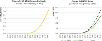
Increasing US R&D spending over the period 2025 to 2035 is expected to boost US R&D knowledge stocks and raise long-run US agricultural productivity growth. Figure 2 shows the annual changes in the knowledge stocks and agricultural TFP growth for the US by taking the differences between “S1 – Baseline” and “S3 – Greater US R&D spending” scenarios. Though R&D spending increases by 7% per year from 2025 to 2035 in scenario S3, notable changes in the knowledge stocks only occur after 2035 and beyond. The change in US knowledge stocks in 2035 is just around 0.07 billion USD, increasing to 3.23 billion by 2050. The changes in US agricultural TFP depend on the changes in US R&D knowledge stocks and the mean, upper and lower values of the R&D stock TFP elasticities. In 2040, the mean, upper, and lower US agricultural TFP growth rates are around 3.0%, 3.9%, and 2.3%, respectively. These rates increase to 17.6% 23.6% and 13.4% in 2050, respectively. Given the distribution of R&D knowledge stocks in Figure 1, most of the gains from greater US R&D investments over the period 2025 to 2035 are likely to be realized after 2050.

Figure 2. Annual changes in US knowledge stocks and agricultural TFP growth.
Despite the lagged effect of R&D spending on productivity growth, greater R&D spending over this period is expected to provide economic gains. Table 2 shows the gross economic benefits under scenario “S3 – Greater US R&D spending” relative to the baseline (S1), evaluated over the period 2017 to 2050. It reports the net present cost and net present benefits of a 7% per year increase in US R&D spending over 2025 to 2035 assuming a discount rate of 3%. The net present cost of scenario S3 is around 85.8 billion USD. The net present benefits are calculated by boosting value of agricultural output in 2017, taken from USDA ERS (2021), using the predicted increase in US agricultural TFP shown in Figure 2. The mean value of the net present benefit is around 173.8 billion USD and is bounded at around 226.9 to 134.6 billion USD. The calculated gains are larger than the costs which suggests that investments in US public agricultural R&D provide gross economic gains. On average, the benefit-cost ratio of this policy is around 2.0 while the internal rate of return (IRR) and modified internal rate of return (MIRR) are around 13.7% and 6.8%, respectively. The range of the benefit-cost ratio is around 2.6 to 1.6. For the IRR and MIRR, the ranges for these rates are around 17.3% and 10.1% and 8.0% and 5.5%, respectively.
Table 2. Greater US R&D spending at 7% per year over 2025 to 2035

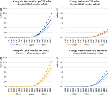
Increasing US R&D spending is expected to generate spillover effects in the rest of the world. Figure 3 shows the changes in agricultural TFP for several regions, indicating that Latin America and Western Europe are expected to benefit more from the R&D spillovers compared to Developed Asia and Oceania + South Asia. These TFP projections depend on the growth in international R&D knowledge stock, which is determined by changes in US R&D spending, and on the regional R&D spillover elasticities.

Figure 3. Annual changes in agricultural TFP growth in key regions due to US R&D spillovers.
Changes in US agricultural production and GHG emissions from 2017 to 2050
Changes in US agricultural production and GHG emissions over the period 2017–2050 under different scenarios are summarized in Table 3. Under the baseline scenario (S1), US agricultural productivity rises by 38.7% while farm output grows by 50.0%. US crop and livestock output expand by about 58.4% and 38.6%, respectively, despite falling supply prices (by −19.0% and −28.7%, respectively). These results show strong farm productivity growth under the baseline improves US producers’ competitiveness and incentivizes agricultural output expansion. However, output expansion results in more land being used in agriculture. Under the baseline, US cropland area expands by 6.7 million hectares (M ha) (by 4.2% relative to 2017). Average annual agricultural GHG emissions in the baseline are around 490.4 million metric tons (M MT) CO2-eq/year, or 1.57 kilograms (kg) CO2-eq/year per USD in farm output.
Table 3. Changes in US and World agricultural production and GHG emissions from 2017 to 2050

Restrictions on farmer input use (S2) result in environmental benefits, but at the expense of lower agricultural output growth and higher food prices. When US crop input use is reduced by 10%, US cropland use contracts by around −7.9 M ha (−4.9%) from 2017 to 2050 and average farm GHG emissions and emissions per output are much lower, at 416.3 M MT CO2-eq/year and at 1.39 kg CO2-eq/year per USD, respectively. However, compared to the baseline, US farm output growth is much slower (growing by 44.3%). US crop production increases by 49.1 % but this is less than the growth under baseline. Livestock output growth is roughly the same as in S1 since input restrictions are only applied to the crop sector. Crop and livestock supply prices still fall (by −15.8% and −28.5%), but less than under the baseline.
With a 7% per year increase in US agricultural R&D spending from 2025 to 2035 (S3), US agricultural productivity and output increase more and prices fall more than under the baseline, but with environmental tradeoffs since increased price competitiveness incentivizes farmers to expand production and use more land and non-land inputs. US agricultural productivity is expected to grow by 62.1%, resulting in significantly faster output growth and declines in supply prices than in the baseline (S1) or reduced input use scenarios (S2). Though average agricultural GHG emissions and emissions per farm output, 486.2 M MT CO2-eq/year, are modestly lower than in S1, US cropland area expands by around 7.0 M ha (by 4.4%). These results suggest that increasing productivity alone is not sufficient to substantially reduce input use and GHG emissions in US agriculture. However, greater productivity leads to much greater GHG efficiency with 1.38 kg CO2-eq/year per USD farm output.
Scenario S4 is a counterfactual scenario of S3 and shows how the absence of international R&D spillovers from US public R&D spending affects the agricultural sector. Without these spillovers, other regions do not benefit from US R&D spending. This results in greater expansion in agricultural production, cropland use, and GHG emissions within the US than under the baseline, as well as a slower decline in crop and livestock prices.
Combining increased R&D spending with reduced farm input use (S5) avoids the adverse tradeoffs of implementing either policy alone. Agricultural output, including crop and livestock production, increases more than under the baseline or reduced input scenarios, though slightly less than under the greater R&D scenario. A similar trend is seen for crop and livestock prices. Unlike S3 where only R&D investment policies are considered, cropland area in S5 contracts by −4.9% (decreasing by 7.8 M ha) as crop producers face constraints in land and non-land input use. Average agricultural GHG emissions are around 410.5 M MT CO2-eq/year while average GHG emissions per output are at 1.22 CO2-eq/year per USD, much lower than under S2 and S3.
Building on S5, scenarios S6 and S7 show the uncertainty in the impact of R&D spending on agricultural productivity growth. These scenarios represent the upper and lower bounds on the expected farm productivity growth from R&D spending, respectively. The results show that US agricultural productivity growth is between 69.7% and 56.7% given a 7% per year increase in US R&D spending over 2025 to 2035. Agricultural output growth is around 68.3% and 58.0% under S6 and S7, respectively. Under S6 where the productivity gains are greater, US crop and livestock output expands by 83.3% and 54.7%, respectively. But even with lower benefits from R&D investments, crop and livestock output growth are still above the baseline at 68.5% and 47.9%, respectively. US crop supply price reduction is between −30.9% and −25.4% while for livestock the change between −42.2% and −37.1%. Note that input restrictions are also imposed under S6 and S7 scenarios. Given this policy, US cropland contracts by around −7.7 and −7.9 M ha, respectively. The upper and lower bounds of average agricultural GHG emissions are around 410.0 and 411.3 M MT CO2-eq/year, respectively. For GHG emissions per output, the bounds are at 1.17 and 1.25 kg CO2-eq/year per USD. The results show that even under the lower bound scenario there are substantial gains in agricultural production and reduction in GHG emissions from the combined policy of increased R&D spending and farm input reduction.
Changes in global agricultural production and GHG emissions from 2017 to 2050
Global markets adjust to changes in US agriculture. Productivity gains from US R&D spending increase the competitive advantage of US farm products while input restrictions make farmers less competitive. At the same time, the rest of the world also benefits from US R&D investments via knowledge spillovers. Table 3 reports the global changes in agricultural production and GHG emissions over the period 2017–2050 under different scenarios.
Under the baseline (S1), global agricultural productivity increases by 40.0% while total farm output rises by 56.2%. World production of livestock grows faster than crop, which shows the impact of changing diets on the composition of agricultural production (around 61.6% and 54.2%, respectively). World supply prices for these commodities are also expected to fall (by −21.8% and −30.2%, respectively). Globally, cropland area is expected to rise by 93.6 M ha (by 6.0% relative to 2017 area). World agricultural emissions from 2017 to 2050 are around 8218.6 M MT CO2-eq/year while GHG emissions per output are at 2.13 kg CO2-eq/year per USD. Note that the global GHG emissions per output are roughly 36% more than the US estimates under S1. This shows that US agriculture is more efficient in terms of GHG emissions per output relative to the world average.
At the global level, the magnitude of the changes across alternative scenarios is much smaller. This is expected since only the US and a few regions benefit from US R&D policies while farm input restriction mandates under S2 and S5 are limited to the US. With limited input use in the US (S2), growth in global agricultural output and declines in prices are comparable to the baseline scenario, though crop prices are projected to be slightly higher. With international trade, the impacts of lower US output growth in the world markets are partly offset by output expansion in the rest of the world. In terms of input use, the restrictions implemented in the US are effective in slowing down global cropland expansion at 81.5 M ha. Under S2, world average agricultural GHG emissions are at 8167.2 M MT CO2-eq/year while GHG emissions per output are at 2.12 kg CO2-eq/year per USD.
Greater US R&D spending results in higher global productivity and production, reduced land use, and GHG emissions, and lower prices than either the baseline or reduced input scenarios. Global farm productivity under S3 increases by 44.3% which leads to output expansion at 57.7%. World livestock production rises faster than crop output with greater US R&D spending (63.5% and 55.5%, respectively). Global average supply prices for these commodities also fall faster than in the baseline (−32.7% and −28.2%, respectively). Even with the expansion in US cropland area in S3, global cropland expansion under this scenario is 18% lower (at 76.7 M ha) than under the baseline. Similarly, average agricultural emissions between 2017 and 2050 are 213.4 MMT CO2-eq/year lower than under the baseline, and emissions per output are 3.5% lower. Global land use and GHG emissions are also lower than in the input restriction scenario (S2). These results show that the accounting of the economic and environmental benefits from US R&D spending policies should consider the production gains and GHG reductions achieved beyond its borders.
In the absence of R&D spillovers (S4), the global gains from US R&D investments are dampened which shows that knowledge transfers to the rest of the world are important co-benefits of any agricultural R&D policy. Global farm productivity and output grow at a slower rate under S4 than under S3. Likewise, the decline in crop and livestock prices is smaller. The environmental gains are also reduced. For instance, global cropland use grows by 86.1 M ha, which is 12% more than when spillovers are considered.
The global outcomes in S5 show that the combined R&D and input restriction policies result in similar or greater output growth and price reduction compared to S1 but greater gains in terms of avoided GHG emissions and cropland expansion compared to S2 and S3 – scenarios where these policies are implemented separately. These results are robust to uncertainties in the productivity gains from US R&D spending, as the outcomes for S6 and S7 indicate (Table 3). Under S5, world agricultural output expands by 57.6% with faster growth in livestock than in crop production (63.5% and 55.3%, respectively). Relative to the baseline, global average supply prices for these goods fall faster over this period (−32.7% and −27.3%, respectively). Around 64.9 M ha of additional cropland (expanding by 4.1%) is needed globally but this is roughly 31% less than the expansion in S1. The rise in agricultural GHG emissions and emissions per output are also dampened (7957.1 M MT CO2-eq/year and 2.05 kg CO2-eq/year per USD). This indicates that the global environmental gains from the combined R&D and input restriction policy are much larger than if these policies were pursued individually even with uncertainty in the impacts of US R&D spending on farm productivity.
Summary and Conclusions
In this study, the economic and environmental benefits from increased US public R&D investments are examined. Empirical estimates from a historical analysis of US R&D spending and agricultural productivity growth as well as technological spillover parameters for selected regions are used. Increasing the growth rate of US R&D investments over the period 2025−2035 by 7% per year could boost US agricultural TFP by 17.6% in 2050. This is projected to generate economic gains within the US over the period 2017 to 2050, accounting for net present benefits and costs. And with technical spillovers, US R&D spending can also be an additional source of farm TFP growth in key world agricultural regions. The impacts of increased US R&D spending at home and abroad are then calculated using a global economic model of agriculture. In addition to the future baseline for period 2017−2050, alternative scenarios are estimated in this study.
In the future baseline, US and global agricultural output are expected to increase, resulting in declining commodity prices, growing cropland area, and GHG emissions. Increasing US R&D spending increases output and price reductions further, while reducing global cropland expansion and GHG emissions. Technological spillovers from the US are important sources of farm productivity for other regions, and these spillovers can enhance the economic and environmental outcomes at the global level. However, as US productivity increases, the competitiveness of US commodities in the world market also improves. This results in greater production and cropland use, limiting the domestic environmental benefits from R&D. Within the US, agricultural GHG emissions can only be reduced effectively when stringent input restrictions are implemented. But by itself, these restrictions can have adverse impacts on US farm production and prices. Greater R&D spending combined with restrictions in input use in the US provide both economic gains from increased production as well as reduced US and global GHG emissions from lower input use. These results show support to strengthen US R&D investment policies, as these show the direct economic benefits from continued agricultural productivity growth and potential synergies with policies that reduce agricultural GHG emissions. These economic and environmental gains are robust even with parameter uncertainties.
Finally, it is important to highlight key limitations of this study for future work. First, the evaluation of the gains in R&D spending is limited. Note that given the 50-year duration of the R&D lag weights, investments in the period 2025−2035 are only fully realized by 2075−2085. Given this, future work should extend the evaluation of the benefits and cost flows and its impact on global agriculture over a longer time horizon. Second, the input restrictions are only implemented in the crop sector which is too narrow since the livestock sector is an important source of farm GHG emissions. Future work should extend input restriction to the livestock sector and explicitly model ruminants and nonruminant livestock since these sectors have different GHG emissions intensities. Ruminants also interact with the crop sector indirectly via competition for land resources. Third, market distortions such as export taxes and import tariffs are not explicitly incorporated in the SIMPLE model. These distortions could likely limit US agricultural trade flows and dampen the indirect impacts of increased US R&D policies via international commodity markets. Finally, there is a need to provide separate estimates of R&D-led TFP growth for the livestock and crop sector. The state-of-the-art focuses on all agriculture. Farming is a multi-output and multi-input activity, and it is quite difficult to isolate the contribution of specific inputs to output growth in the livestock and crop sector. However, developing separate R&D TFP parameter estimates could be useful in justifying how R&D spending in agriculture is optimized across these sectors to curb overall farm GHG emissions.
Supplementary material
The supplementary material for this article can be found at https://doi.org/10.1017/aae.2023.29.
Data availability statement
The data that support the findings of this study are available at https://doi.org/10.5281/zenodo.8148398
Acknowledgements
The author thanks Daniel Blaustein-Rejto for feedback and comments.
Financial support
This work was supported by the Breakthrough Institute.
Competing interests
Uris Lantz C. Baldos declare none.
Conceptualization, U B; Methodology, U B; Formal Analysis, U B; Data Curation, U B; Writing – Original Draft, U B, Writing – Review and Editing, U B, Supervision, U B; Funding Acquisition, U B.


 Open access