


1. Introduction
The production function is a technological relationship between inputs and output. In the standard neoclassical production function approach, it is assumed that producers do not face any uncertainty (Chambers, Reference Chambers1988). However, certainty is rarely the case in reality because risk and uncertainty are inescapable factors in production. Footnote 1 Hence, they affect input use decisions, which in turn affect the production of outputs. Footnote 2
Many approaches have relaxed the perfect certainty assumption. A frequently used approach, which has been applied for many decades, is the Just–Pope production function approach, which, for a given set of inputs, allows inputs to increase or decrease production risk, measured by the variance of output (Just and Pope, Reference Just and Pope1978, Just and Pope, Reference Just and Pope1979). Footnote 3 From an econometric point of view, the Just and Pope approach is a heteroskedastic model in which heteroskedasticity (variance of the production error) is a function of inputs (e.g., Asche and Tveterås, Reference Asche and Tveteras1999). Conditional output variance does not affect production decisions based on expected profit or expected utility of profit; it simply makes the error term heteroskedastic. Footnote 4 This consequence is counterintuitive because the presence of risk is likely to affect input use and, therefore, output. Herein, the Just–Pope production function formulation is extended to include technical inefficiency, which affects mean output (Battese et al., Reference Battese, Rambaldi and Wan1997; Kumbhakar, Reference Kumbhakar2002). Footnote 5 A limitation of the Just–Pope production function formulation is that it does not take into account producers’ behavior toward risk (Kumbhakar, Reference Kumbhakar2002). Thus, input elasticities and returns to scale, among other things, are treated as not affected by producers’ risk perceptions, which is not realistic. Footnote 6
The state-contingent production framework, advocated by Chambers and Quiggin (Reference Chambers and Quiggin2000), drawing on the work of Arrow and Debreu (Reference Arrow and Debreu1954), allows input choices to have different consequences in different states of nature. The consequences of risky choices are analyzed as depending upon which of the possible uncertain states of the world occurs. This is not a property of conventional production theory, in which inputs are assumed to play the same role regardless of which state occurs. Although the theory of a state-contingent production function is well established, applications in agriculture are somewhat limited because empirical implementation is very data demanding. Footnote 7
In a recent study, Lien et al. (Reference Lien, Kumbhakar and Hardaker2017) accounted for risk in productivity analysis by including risk indices (a group of risk-related variables) in a translog (TL) production function (or input distance function). Through the functional form, with interactions between the input variables and the risk-related variables, the effects of risk-related variables on productivity were investigated. As with the Just–Pope approach, a problem with this approach is that the risk-related variables are different from the input variables because they are not standard inputs. Moreover, mathematically speaking, one cannot simply identify the input variables from the risk-related variables by using different names.
Another framework to address farmers’ risk and risk attitudes and how these affect their risk management decision-making and diversification strategies is a system approach consisting of a production function and the first-order conditions of the expected utility-of-profit maximization. In such a framework, it is possible to jointly estimate both the technology, producers’ risk attitude, and effects of production risk. For example, Kumbhakar and Tveterås (Reference Kumbhakar and Tveteras2003) introduced a parametric econometric model that estimates technology, production risk, and risk attitude simultaneously. Kumbhakar (Reference Kumbhakar2002) extended that model to simultaneously estimate technical efficiency. Kumbhakar and Tsionas (Reference Kumbhakar and Tsionas2010) introduced a nonparametric model that simultaneously estimated technology, production risk, and producers’ risk attitudes without making any distributional assumptions. Ballivian and Sickles (Reference Ballivian and Sickles1994) estimated a system of input demand and output supply functions using a quadratic profit function. Without prices and variability in the price data, which is the case for our study, it is not possible to use the approaches mentioned in this paragraph. Furthermore, in the framework discussed here, the production function is included in the model framework to derive the risk attitude function. Therefore, the estimated production function is not risk adjusted.
Chavas and Shi (Reference Chavas and Shi2015) used conditional quantile regression to assess production risk in agriculture, or more precisely, the distribution of the yield and the effects that different input variables have on the conditional distribution. They also placed the estimates from the conditional quantile regression into an expected utility model, and then they assumed the degree of farmers’ risk aversion. Using the estimated parameters from a quantile regression and the assumed degree of risk aversion in a simulation study, they were able to calculate the certainty equivalent output, which they used as a risk-adjusted output measure in the production function, to assess whether or not to use genetically modified (GM) seed agricultural technology. With their approach, Chavas and Shi (Reference Chavas and Shi2015) were also able to disentangle the certainty equivalent into mean effects and a risk premium (measuring the cost of risk).
In this paper, we introduce an alternative approach to modeling the effects of the input choices (or how elasticities change) in the presence of risky production conditions. In the first step, to account for farmers’ risk aversion, we used data from an experiment to estimate individual farmers’ degrees of risk aversion and their risk premium and to calculate their certainty equivalent (CE) gross revenues. In the second step, we use the CE of gross revenue as output (adjusted for output risk), instead of observed gross revenue (Y), in specifying the production function. In that way, we obtain a certainty equivalent-adjusted or risk-adjusted production function. Footnote 8 Thus, the effect of the inputs on returns will automatically be risk adjusted, i.e., we obtain risk-adjusted marginal effects and risk-adjusted input elasticities for each farmer. In that way, we obtain a decision support model that accounts for the individual farmer’s risk attitude.
Note that under our approach, we are not modeling directly the production risk of inputs used, as the expected utility-of-profit framework does. Still, we do it indirectly (through the estimated risk-adjusted marginal effect of inputs), by accounting for producers’ risk behavior in our production function. To the best of our knowledge, our approach of including risk attitude in the production function framework and then also estimating risk-adjusted elasticities has not been examined in the literature.
We illustrate our method using farm-level data from organic basmati rice (OBR) smallholders in India. A survey completed in 2015 collected data from 880 smallholder households in the states of Punjab, Haryana, and Uttarakhand in the northern part of India. The data set includes various aspects of the farming business and also data from a gamble-choice elicitation method to elicit an individual farmer’s risk attitude.
2. Modeling Approaches
2.1. Modeling Framework
For a crop farmer, the input decisions are made before the harvest. Consequently, the yield and returns that a crop farmer obtains will always be risky for several reasons, such as weather risks, pest and disease risk, and market risks. The realized postharvest output (Y) the farmer obtains is seldom the same as the anticipated output at planting/sowing. For every farmer (or decision-maker in general) faced with risky payoffs, e.g., the payoff from farming, there is a sum of money ‘for sure’ that would make her indifferent between facing the risk or accepting the sure sum. In the case of farming, this sure sum is the lowest sure gross revenue that the farmer would be willing to accept to sell a desirable risky prospect or the highest sure gross revenue the farmer would pay to avoid an undesirable risky prospect. This sure sum is CE and is the guaranteed amount of cash that a farmer would consider as having the same amount of desirability as a risky payoff/gross revenue. The difference between the CE and the expected value of a risky prospect, known as the risk premium, is a measure of the cost of the combined effects of risk and risk aversion (Chavas and Shi, Reference Chavas and Shi2015; Hardaker et al., Reference Hardaker, Lien, Anderson and Huirne2015). If we have measures of risk and risk aversion, we are able to convert farmers’ observed gross revenue to the CE of gross revenue. Using the CE of gross revenue as the output in the production function, we are then able to estimate a CE-adjusted or risk-adjusted production function and obtain risk-adjusted marginal effects, elasticities, and economies of scale measures. In general, CEs will vary among farmers, even for the same risky prospect, because farmers seldom have identical attitudes to risk (utility functions), and they may also hold different views about the chances of better or worse outcomes occurring (Pennings and Garcia, Reference Pennings and Garcia2001; Hardaker et al., Reference Hardaker, Lien, Anderson and Huirne2015). The advantage of working with the CE output is that it will avoid the complicated procedure of estimating the input demand system based on maximizing the expected utility of profit, assuming a parametric form of the utility function (Ballivian and Sickles, Reference Ballivian and Sickles1994) or approximating it (Kumbhakar, Reference Kumbhakar2002; Kumbhakar and Tveterås, Reference Kumbhakar and Tveteras2003).
Based on these ideas, we introduce the CE-adjusted or risk-adjusted production function below. Different specifications of that model will be presented after the description of how to estimate the CE.
2.2. Estimating the Certainty Equivalent
To specify a CE- or risk-adjusted production function, we need to convert the dependent variable from farmers’ observed monetary gross revenue to farmers’ risk-adjusted gross revenue. As mentioned above, CE gross revenue is defined as $CE = Y- RP$
, where Y is gross revenue from outputs and RP is risk premium, which is the implicit cost of private risk-taking. RP is the amount of money that makes the farmer indifferent between the risky gross revenue
$CE = Y- RP$
, where Y is gross revenue from outputs and RP is risk premium, which is the implicit cost of private risk-taking. RP is the amount of money that makes the farmer indifferent between the risky gross revenue $\left( Y\right)$
and the certain risk-adjusted gross revenue
$\left( Y\right)$
and the certain risk-adjusted gross revenue $\left( {CE} \right)$
.
$\left( {CE} \right)$
.
One measure of risk premium is the Arrow–Pratt approximation, developed independently by Arrow (Reference Arrow1963) and Pratt (Reference Pratt1964), and is defined as
 $$RP = {1 \over 2} \times ARA \times Var\left( Y\right),$$
where ARA is the degree of absolute risk aversion for the farmer (decision-maker) with respect to wealth. Absolute risk aversion is a measure of farmer’s/decision-maker’s reaction to risk relating to changes in their wealth. $Var\left( Y\right)$
is the variance of gross revenue (Y).
$Var\left( Y\right)$
is the variance of gross revenue (Y).
Thus, the CE of gross revenue in a risky situation can be approximated by
 $$CE = Y- {1 \over 2} \times ARA \times Var\left( Y\right).$$ $Var\left( Y\right)$
are environmental variables in the production. In other words, the CE in this study is approximated by
$Var\left( Y\right)$
are environmental variables in the production. In other words, the CE in this study is approximated by
 $$CE = Y- {1 \over 2} \times ARA \times Var(Y|{\rm{Z}}).$$
To make the CE approach operational, we need estimates of ARA and $Var(Y|{\rm{Z}})$
. The conditional variance,
$Var(Y|{\rm{Z}})$
. The conditional variance, $Var(Y|{\rm{Z}})$
, was estimated with a nonparametric estimator. We first estimated the conditional mean for output,
$Var(Y|{\rm{Z}})$
, was estimated with a nonparametric estimator. We first estimated the conditional mean for output, $E(Y|{\rm{Z}})$
, for each observation, by nonparametric regression. Then, we calculated the conditional variance of output for each observation/farm using the formula
$E(Y|{\rm{Z}})$
, for each observation, by nonparametric regression. Then, we calculated the conditional variance of output for each observation/farm using the formula $Var(Y|{\rm{Z}}) = {[Y - E(Y|{\rm{Z}})]^2}$
.
Footnote 9
$Var(Y|{\rm{Z}}) = {[Y - E(Y|{\rm{Z}})]^2}$
.
Footnote 9
The absolute risk-aversion coefficient, ARA, often named the Arrow–Pratt coefficient of absolute risk aversion, is determined by the curvature of a utility function, which is defined by dividing the second derivative by the first derivative of a defined utility function (Arrow, Reference Arrow1963; Pratt, Reference Pratt1964). A utility function can be defined with different payoff measures (e.g., losses and gains, income, and wealth). Any measure of risk aversion is specific to the particular payoff measure over which the measure is defined (Meyer and Meyer, Reference Meyer and Meyer2006). Following Arrow (Reference Arrow1963) and Pratt (Reference Pratt1964), it is also quite common to maximize the expected utility of wealth (W), which defines the absolute risk-aversion measure for a change in wealth. Furthermore, it is generally accepted that the absolute risk-aversion coefficient (ARA) with respect to wealth will decrease with increases in wealth because farmers/decision-makers can better afford to take risks as they get richer (Hardaker et al., Reference Hardaker, Lien, Anderson and Huirne2015, Ch. 5). In other words, an assumption about decreasing absolute risk aversion (DARA) seems reasonable. Note also that the absolute risk-aversion measure depends on the monetary units of wealth, and measures derived from different currency units are not comparable. The currency problem is overcome using the relative risk-aversion (RRA) measure, defined as $RRA = ARA \times W$
. A power utility function has the property of constant relative risk aversion (CRRA), meaning that the relative risk-aversion measure is constant for all wealth levels. And CRRA functions also feature DARA, which, as mentioned, is a reasonable property. We used estimates of individual farmers’ degree of CRRA (ranked from 1 (hardly risk averse) to 4 (very risk averse)), which we obtained from the survey used in this study (described below). With these estimates, we simply converted the relative risk-aversion coefficient to the absolute risk-aversion coefficient, (ARA), using the level of the farmers’ wealth
$RRA = ARA \times W$
. A power utility function has the property of constant relative risk aversion (CRRA), meaning that the relative risk-aversion measure is constant for all wealth levels. And CRRA functions also feature DARA, which, as mentioned, is a reasonable property. We used estimates of individual farmers’ degree of CRRA (ranked from 1 (hardly risk averse) to 4 (very risk averse)), which we obtained from the survey used in this study (described below). With these estimates, we simply converted the relative risk-aversion coefficient to the absolute risk-aversion coefficient, (ARA), using the level of the farmers’ wealth $\left( W\right)$
from a survey (see below) via the formula
$\left( W\right)$
from a survey (see below) via the formula $ARA = RRA/W$
.
$ARA = RRA/W$
.
Finally, using the estimates of $Var(Y|{\rm{Z}})$
and ARA, we calculated the CE (equation (3) above) and used it as the output variable (instead of Y, which is gross revenue) in the production function (see below), to define the production function accounting for the decision-makers risk attitudes.
$Var(Y|{\rm{Z}})$
and ARA, we calculated the CE (equation (3) above) and used it as the output variable (instead of Y, which is gross revenue) in the production function (see below), to define the production function accounting for the decision-makers risk attitudes.
2.3. Empirical Models
Both parametric and nonparametric modeling frameworks can be used to estimate the CE production function model. Below, we use the nonparametric specification, and so avoid making explicit assumptions about the functional form (such as a linear model), as is required for a parametric specification. In addition to the CE nonparametric function (where the risk-adjusted gross revenue is output), we also include, as a benchmark, the standard nonparametric production function (where the observed gross revenue is output). In the Appendix, we provide the specification of, and results for, two parametric production functions; with observed gross revenue as output and with CE gross revenue as output.
The nonparametric standard (risk-unadjusted) production function (4) [Model 1] and nonparametric CE-adjusted production function (5) [Model 2] are specified as
 $${Y_i} = f\left( {{{\rm{X}}_i}} \right) + {v_i},$$
 $$C{E_i} = {f_{CE}}\left( {{{\rm{X}}_i}} \right) + v_i^{CE},$$
where Yi is the logarithm of output (gross revenue) for farm $i{\rm{\;}}\left( {i = 1, \cdots ,n} \right)$
,
$i{\rm{\;}}\left( {i = 1, \cdots ,n} \right)$
, $C{E_i}$
is the logarithm of the CE output (gross revenue) for farm i,
$C{E_i}$
is the logarithm of the CE output (gross revenue) for farm i, $f\left( {{{\rm{X}}_i}} \right)$
is the nonparametric functional form, and Xi is a vector of inputs. Finally,
$f\left( {{{\rm{X}}_i}} \right)$
is the nonparametric functional form, and Xi is a vector of inputs. Finally, ${v_i}$
is the random error term.
${v_i}$
is the random error term.
2.4. Specification of the Empirical Models
Model 1, the nonparametric production function, as described in equation (4), is estimated by constructing a relationship between Y and ${X_j}$
based on weighted averages, so that we do not have to specify a specific functional form. A general class of local nonparametric regression models of (4) can be written as
${X_j}$
based on weighted averages, so that we do not have to specify a specific functional form. A general class of local nonparametric regression models of (4) can be written as
 $$\widetilde m\left( X\right) = \mathop \sum \limits_{i = 1}^N \,w\left( {{X_i},X} \right){Y_i},$$
where $w\left( {{X_i},X} \right)$
represents the weight assigned to the
$w\left( {{X_i},X} \right)$
represents the weight assigned to the ${i^{{\rm{th}}}}$
observation Yi, with the weight depending on the distance of the sample point Xi from the point X (Li and Racine, Reference Li and Racine2004). Different nonparametric estimators can be defined using equation (6). One particular class of estimators is the kernel estimator, as is used in our study, which defines the weighting function as
${i^{{\rm{th}}}}$
observation Yi, with the weight depending on the distance of the sample point Xi from the point X (Li and Racine, Reference Li and Racine2004). Different nonparametric estimators can be defined using equation (6). One particular class of estimators is the kernel estimator, as is used in our study, which defines the weighting function as
 $$w\left( {{X_i},X} \right) = {{K\left( {{{{X_i} - X} \over h}} \right)} \over {\mathop \sum \nolimits_{i = 1}^N \,K\left( {{{{X_i} - X} \over h}} \right)}},$$
where $K\left( \cdot \right)$
is a multivariate kernel, and h is a smoothness parameter called the bandwidth that determines how many Xi around X are used in the kernel function. There are several ways to specify the kernel function (for example, Gaussian, uniform, Epanechnikov, etc.) and several ways to specify the bandwidth (for instance, least-squares cross-validation or likelihood cross-validation). For details on these issues, see, for example, Li and Racine (Reference Li and Racine2004) and Henderson and Parmeter (Reference Henderson and Parmeter2015). In our study, we chose Gaussian kernel functions and least-squares cross-validation to select bandwidths.
$K\left( \cdot \right)$
is a multivariate kernel, and h is a smoothness parameter called the bandwidth that determines how many Xi around X are used in the kernel function. There are several ways to specify the kernel function (for example, Gaussian, uniform, Epanechnikov, etc.) and several ways to specify the bandwidth (for instance, least-squares cross-validation or likelihood cross-validation). For details on these issues, see, for example, Li and Racine (Reference Li and Racine2004) and Henderson and Parmeter (Reference Henderson and Parmeter2015). In our study, we chose Gaussian kernel functions and least-squares cross-validation to select bandwidths.
For nonparametric models, there are no parameters, and even when they are approximated by a higher order polynomial, the parameters do not have any direct interpretation. For these models, the interest lies in the gradients, which are the input elasticities, ${{\partial Y} \over {\partial {X_j}}}$
.
Footnote 10
These input elasticities are observation-specific, and we can compute the mean and/or quantiles or provide density plots of them.
${{\partial Y} \over {\partial {X_j}}}$
.
Footnote 10
These input elasticities are observation-specific, and we can compute the mean and/or quantiles or provide density plots of them.
For Model 2, the nonparametric CE-adjusted production function, Y, is replaced with CE in equation (5), and everything else is exactly the same as for Model 1.
Although nonparametric models are very flexible, the price one must pay is a higher probability of empirical violations of economic conditions. For example, one cannot guarantee positive input elasticities for each variable at every data point. One way to mitigate this potential problem is to consider constrained estimation. There is an extensive literature on constrained nonparametric estimation (see Henderson and Parmeter, Reference Henderson and Parmeter2015, Chapter 12, for an overview). For the nonparametric Models 1 and 2 (equations (4) and (5)), we imposed monotonically restricted gradient estimates using the approach outlined in Parmeter et al. (Reference Parmeter, Sun, Henderson and Kumbhakar2014). The idea with this approach is to reweight the dependent variable as little as possible, but at the same time, to avoid negative input elasticities.
3. Data for Application of the Models
We use a primary survey of smallholder households, conducted in 2015 in the states of Punjab, Haryana, and Uttarakhand in the northern part of India. Farmers were chosen randomly from a list of farmers engaged in OBR production. A total of 880 OBR farmers were included in our analyzed sample (we omitted 69 observations because of missing data or outliers). Of these, 375 were located in Punjab (196 from the Amritsar District and 179 from the Patiala District), 334 were in Haryana (170 from the Karnal District and 164 from the Kaithal District), and 171 were from Uttarakhand (from the Dehradun District). The survey included data on various aspects of the farming business, such as assets, costs, income, the economics of cultivation, social network, information on contract farming, adoption of best practices, risk perception, and risk aversion.
We specify the production function, with gross revenue as output, $\left( Y\right)$
, and three inputs. The following three inputs are used: land
$\left( Y\right)$
, and three inputs. The following three inputs are used: land $\left( {{X_1}} \right)$
, measured in acres; labor
$\left( {{X_1}} \right)$
, measured in acres; labor $\left( {{X_2}} \right)$
, measured in man-years equivalent; and other costs (X 3), measured in rupees. Other costs include costs of fertilizer, irrigation, weeding, pesticides, harvesting, marketing, etc.
$\left( {{X_2}} \right)$
, measured in man-years equivalent; and other costs (X 3), measured in rupees. Other costs include costs of fertilizer, irrigation, weeding, pesticides, harvesting, marketing, etc.
In the literature, several techniques have been used to elicit decision-makers’ or farmers’ risk attitudes (see Binswanger, Reference Binswanger1980; Charness et al., Reference Charness, Gneezy and Imas2013; Hellerstein et al., Reference Hellerstein, Higgins and Horowitz2013; Saastamoinen, Reference Saastamoinen2015; Charness and Viceisza, Reference Charness and Viceisza2016; Vollmer et al., Reference Vollmer, Hermann and Mußhoff2017; Iyer et al., Reference Iyer, Bozzola, Hirsch, Meraner and Finger2020; Bozzola and Finger, Reference Bozzola and Finger2021). Iyer et al. (Reference Iyer, Bozzola, Hirsch, Meraner and Finger2020) distinguished between three risk-attitude measurement methods: 1) econometric estimates based on farm-level data; 2) methods based on self-reports of multi-item scales; and 3) gamble-choice elicitation methods. As suggested by Just and Just (Reference Just and Just2011), in the present study, risk attitude was measured using a gamble-choice elicitation method. More specifically, the last one of these three above-mentioned alternatives was used in our survey to construct the variable to measure attitude to risk $\left( {{Z_1}} \right)$
, based on the context-free ordered lottery selection approach (Eckel and Grossman, Reference Eckel and Grossman2008). The context-free ordered lottery selection approach has also been used to elicit risk attitude among managers of natural resources (e.g., Reynaud and Couture, Reference Reynaud and Couture2012; Brunette et al., Reference Brunette, Foncel and Kere2017).
Footnote 11
In the survey, the farmers had to select the preferred gamble from six alternatives (see Table 1). For each farmer’s response, we calculated a coefficient of constant relative risk aversion
$\left( {{Z_1}} \right)$
, based on the context-free ordered lottery selection approach (Eckel and Grossman, Reference Eckel and Grossman2008). The context-free ordered lottery selection approach has also been used to elicit risk attitude among managers of natural resources (e.g., Reynaud and Couture, Reference Reynaud and Couture2012; Brunette et al., Reference Brunette, Foncel and Kere2017).
Footnote 11
In the survey, the farmers had to select the preferred gamble from six alternatives (see Table 1). For each farmer’s response, we calculated a coefficient of constant relative risk aversion $\left( {CRRA} \right)$
. For
$\left( {CRRA} \right)$
. For ${Z_1} \gt 3.0$
, we used
${Z_1} \gt 3.0$
, we used $CRRA = 3.5$
; for the range
$CRRA = 3.5$
; for the range $(1.0 \lt {Z_1} \lt 3.0)$
, we used
$(1.0 \lt {Z_1} \lt 3.0)$
, we used $CRRA = 2.0$
; for the range
$CRRA = 2.0$
; for the range $(0.6 \lt {Z_1} \lt 1.0)$
, we used
$(0.6 \lt {Z_1} \lt 1.0)$
, we used $CRRA = 0.8$
; for the range
$CRRA = 0.8$
; for the range $(0.4 \lt {Z_1} \lt 0.6)$
, we used
$(0.4 \lt {Z_1} \lt 0.6)$
, we used $CRRA = 0.5$
; for the range
$CRRA = 0.5$
; for the range $(0.0 \lt {Z_1} \lt 0.4)$
, we used
$(0.0 \lt {Z_1} \lt 0.4)$
, we used $CRRA = 0.2$
; and for
$CRRA = 0.2$
; and for $\left( {{Z_1} = 0.0} \right)$
, we used
$\left( {{Z_1} = 0.0} \right)$
, we used $CRRA = 0.0$
, i.e., risk neutral. Figure 1 shows the distribution of the respondents. About 29% of the farmers chose the risk-neutral gamble.
$CRRA = 0.0$
, i.e., risk neutral. Figure 1 shows the distribution of the respondents. About 29% of the farmers chose the risk-neutral gamble.
Table 1. Eliciting risk preferences gamble

Notes: $\left( i \right)$
The constant relative risk-aversion (CRRA) range is estimated with the CRRA function
$\left( i \right)$
The constant relative risk-aversion (CRRA) range is estimated with the CRRA function $U = \displaystyle{{\left( {payof{f^{\left( {1 - r} \right)}}} \right)} \over {\left( {1 - r} \right)}}$
. The CRRA limit is the value of r that produces the same utility for Gamble X and Gamble
$U = \displaystyle{{\left( {payof{f^{\left( {1 - r} \right)}}} \right)} \over {\left( {1 - r} \right)}}$
. The CRRA limit is the value of r that produces the same utility for Gamble X and Gamble $X + 1$
.
$X + 1$
.
(ii) Source: Authors’ calculation.

Figure 1. Distribution of the respondents/farmers on reported risk attitude.
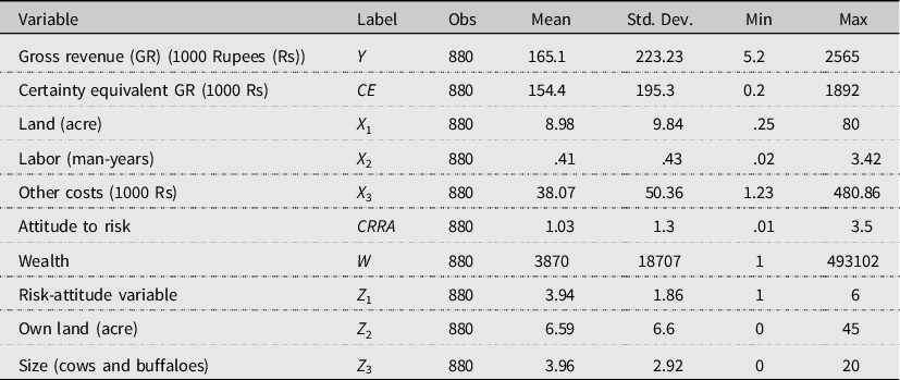
Table 2 presents the descriptive statistics of the variables used in the analysis. The average farm size is about nine acres, but there is significant variability in farm size. Gross revenue from OBR farming averages INR $165.1$
Footnote 12
, while CE gross revenue (CE) at the mean is INR 154.4. In other words, there is an average risk premium of INR
$165.1$
Footnote 12
, while CE gross revenue (CE) at the mean is INR 154.4. In other words, there is an average risk premium of INR $10.7$
(
$10.7$
( $165.1 - 154.4$
), or 6.9% of the observed gross revenue.
Footnote 13
Additionally, other costs show significant variability among OBR farmers. Other costs for OBR smallholders’ average is INR
$165.1 - 154.4$
), or 6.9% of the observed gross revenue.
Footnote 13
Additionally, other costs show significant variability among OBR farmers. Other costs for OBR smallholders’ average is INR $38.1$
. Finally, the estimates of attitude toward risk (CRRA) reveal that OBR smallholders are slightly risk averse, on average, with a CRRA of
$38.1$
. Finally, the estimates of attitude toward risk (CRRA) reveal that OBR smallholders are slightly risk averse, on average, with a CRRA of $1.03$
.
Footnote 14
$1.03$
.
Footnote 14
Table 2. Descriptive statistics $\left( {N = 880} \right)$
4. Results
As mentioned in Subsection 2.4, nonparametric models are flexible, but they have a high probability of violating economic restrictions for the estimated function. With the unconstrained nonparametric estimator, both Model 1 and Model 2 had negative input elasticities for land, labor, and other costs. Footnote 15 These negative values are counterintuitive and are not consistent with production theory. Hence, we present below the results based on the constrained nonparametric estimator for both Models 1 and 2. In the constrained models, we imposed restrictions to make all the input elasticities nonnegative at every point. Table 3 shows the estimated input elasticities, while Figure 2 shows the distribution of the elasticities and RTS.
Table 3. Input elasticities results for the nonparametric standard production function (Model 1) and nonparametric CE production function (Model 2)
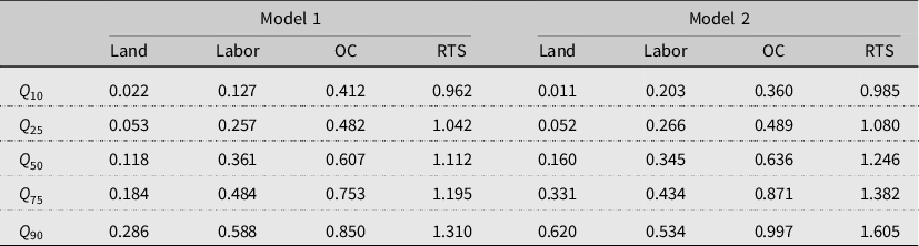
Notes: OC = Other costs, RTS = Returns to scale.

Figure 2. Density plot of input elasticities for land, labor, other costs, and RTS for the nonparametric standard production function (Model 1, in red) and nonparametric risk-adjusted (CE) production function (Model 2, in blue).
The results for the nonparametric standard production function (Model 1) in Table 3 show that, at the median, other costs (materials) have the highest input elasticity $\left( {0.61} \right)$
, labor the second highest
$\left( {0.61} \right)$
, labor the second highest $\left( {0.36} \right)$
, and land the lowest
$\left( {0.36} \right)$
, and land the lowest $\left( {0.12} \right)$
. Furthermore, we find that OBR farms, at the median, are operating under increasing RTS. In other words, a 1% increase in all inputs increases rice output by about 1.11%. Therefore, the results confirm that most OBR producers can benefit from an expansion of operated acreage, except for the farms that are in the bottom 10%. Although theoretically true, the RTS results may not mean much practically because the land is a limiting factor, and in most cases, cannot be increased like labor and materials can.
$\left( {0.12} \right)$
. Furthermore, we find that OBR farms, at the median, are operating under increasing RTS. In other words, a 1% increase in all inputs increases rice output by about 1.11%. Therefore, the results confirm that most OBR producers can benefit from an expansion of operated acreage, except for the farms that are in the bottom 10%. Although theoretically true, the RTS results may not mean much practically because the land is a limiting factor, and in most cases, cannot be increased like labor and materials can.
The results from the different quantiles show that the input elasticities and RTS vary depending on at what point of the distribution each of the estimates are evaluated. For example, in Model 1, the input elasticity of labor at the ${10^{th}}$
percentile is
${10^{th}}$
percentile is $0.13$
, while at the
$0.13$
, while at the ${90^{th}}$
percentile, it is
${90^{th}}$
percentile, it is $0.59$
. The results also suggest that the marginal impact of labor on rice output is heterogeneous and increases monotonically across quantiles. We observe similar relationships for land and other inputs. The distribution of RTS estimates also shows that farms in the
$0.59$
. The results also suggest that the marginal impact of labor on rice output is heterogeneous and increases monotonically across quantiles. We observe similar relationships for land and other inputs. The distribution of RTS estimates also shows that farms in the ${10^{{\rm{th}}}}$
percentile have decreasing RTS (
${10^{{\rm{th}}}}$
percentile have decreasing RTS ( $0.96$
), while farms at the
$0.96$
), while farms at the ${90^{{\rm{th}}}}$
percentile operate under increasing RTS (
${90^{{\rm{th}}}}$
percentile operate under increasing RTS ( $1.31$
).
$1.31$
).
Note that the results and relationships from Model 1 in Table 3, discussed above, assume perfect knowledge of output at the time of harvest. In other words, farmers have certainty with regard to output, and therefore, the elasticities estimated in Model 1 reflect this. However, this is a strong and unrealistic assumption. The realized outputs of farmers postharvest are (typically) not equal to the outputs they expected at planting/sowing.
Thus, in Model 2, the output variable Y is replaced with CE in the production function. The estimates are reported in the right panel of Table 3. An important observation is that adjusting output to CE to accommodate the farmers’ risk attitude clearly influences the estimates. For our sample of OBR producers, the elasticities of land, labor, and other costs are higher than the estimates in Model 1 at the mean, when accounting for the farmers’ risk attitude. However, the results are mixed, for some quantiles, the elasticities are lower with Model 2, while for others, the opposite is true. Model 2 in Table 3 reveals that a 1% increase in all inputs increases rice output by about 0.99% at the ${10^{{\rm{th}}}}$
percentile and by about 1.61% at the
${10^{{\rm{th}}}}$
percentile and by about 1.61% at the ${90^{{\rm{th}}}}$
percentile. Therefore, the results confirm that most OBR producers can benefit from an expansion in operated acreage. Similarly to Model 1, the estimates of the input elasticities and RTS vary across quantiles.
${90^{{\rm{th}}}}$
percentile. Therefore, the results confirm that most OBR producers can benefit from an expansion in operated acreage. Similarly to Model 1, the estimates of the input elasticities and RTS vary across quantiles.
To obtain a better understanding of the results obtained from the nonparametric method, we plot the input elasticities and RTS for Models 1 and 2 and report them in Figure 2. The plots are overlaid so that the differences are easy to visualize. Density plots of the input elasticities for land, labor, other costs, and RTS for Model 1 (2) are in red (blue).
The differences in elasticity estimates vary between Model 1 and Model 2. Figure 2 shows that to some degree, the elasticity estimates for land and labor are similar regardless of a farmer’s risk attitude. However, Figure 2 (bottom two graphs) shows that the elasticity estimates of other costs and RTS are higher when accounting for a farmer’s risk attitude (Model 2). The adjustment of risk-attitude results in higher RTS estimates, in general, implying that OBR producers will benefit from an expansion in the scale of their operations. Figure 2 shows a larger variability for the risk-adjusted elasticity estimates (Model 2) than for those from the unadjusted model (Model 1). However, for labor input, the variability in elasticity decreases after accounting for the farmers’ degree of risk aversion. As shown in Table 2, the elasticity of labor increases for farms that are in the bottom 10% and 25% ( ${10^{th}}$
and
${10^{th}}$
and ${25^{th}}$
percentiles) of the elasticity distribution. Our findings may indicate that the share of labor increases when one accounts for the farmers’ degree of risk aversion. Finally, the land elasticity in Figure 2 is clearly truncated because the unconstrained nonparametric model has a large number of negative land elasticities. In that respect, our finding is consistent with other studies of developing countries that have estimated negative land elasticities (Evenson et al., Reference Evenson, Pray and Rosegrant1998; Kawagoe et al., Reference Kawagoe, Hayami and Ruttan1985; Fulginiti and Perrin, Reference Fulginiti and Perrin1998). Our findings provide evidence of an inverse relationship between farm size and rice productivity, which has been observed in many developing countries including those in Africa (see Barrett, Reference Barrett1996; Kimhi, Reference Kimhi2006; Carletto et al., Reference Carletto, Savastano and Zezza2013) and South Asia (see Heltberg, Reference Heltberg1998; Benjamin and Brandt, Reference Benjamin and Brandt2002; Gaurav and Mishra, Reference Gaurav and Mishra2015; Gautam and Ahmed, Reference Gautam and Ahmed2019).
${25^{th}}$
percentiles) of the elasticity distribution. Our findings may indicate that the share of labor increases when one accounts for the farmers’ degree of risk aversion. Finally, the land elasticity in Figure 2 is clearly truncated because the unconstrained nonparametric model has a large number of negative land elasticities. In that respect, our finding is consistent with other studies of developing countries that have estimated negative land elasticities (Evenson et al., Reference Evenson, Pray and Rosegrant1998; Kawagoe et al., Reference Kawagoe, Hayami and Ruttan1985; Fulginiti and Perrin, Reference Fulginiti and Perrin1998). Our findings provide evidence of an inverse relationship between farm size and rice productivity, which has been observed in many developing countries including those in Africa (see Barrett, Reference Barrett1996; Kimhi, Reference Kimhi2006; Carletto et al., Reference Carletto, Savastano and Zezza2013) and South Asia (see Heltberg, Reference Heltberg1998; Benjamin and Brandt, Reference Benjamin and Brandt2002; Gaurav and Mishra, Reference Gaurav and Mishra2015; Gautam and Ahmed, Reference Gautam and Ahmed2019).
In Figure 3, scatter plots for Models 1 and 2 graphically illustrate the differences between the models’ elasticity estimates for the same farms. A perfect match between Model 1 and Model 2 would show up as a straight line in the graph, and not as a scatter of points. That is not the case, however, as the results for Models 1 and 2 are in general quite different, and these two models also show quite inconsistent elasticity estimates, meaning that standard input elasticities often vary significantly from risk-adjusted/welfare-adjusted input elasticities. The trend lines show a roughly linear relationship between the elasticity estimates for Models 1 and 2. The trend lines confirm the visual inspections of the graphs and show a ${R^2}$
between 0.69 and 0.92. From the trend lines, we also observe estimated slope parameters above one for land, other costs, and RTS, meaning that, in general, Model 2 estimates higher risk-adjusted/welfare-adjusted input elasticities than Model 1’s standard input elasticity estimates, for the same farms. For labor, the opposite is true; the trend line shows a slope parameter below one. This means that the risk-adjusted/welfare-adjusted input elasticity estimates for labor are, in general, lower than the standard input elasticity estimates for labor for the same farms.
${R^2}$
between 0.69 and 0.92. From the trend lines, we also observe estimated slope parameters above one for land, other costs, and RTS, meaning that, in general, Model 2 estimates higher risk-adjusted/welfare-adjusted input elasticities than Model 1’s standard input elasticity estimates, for the same farms. For labor, the opposite is true; the trend line shows a slope parameter below one. This means that the risk-adjusted/welfare-adjusted input elasticity estimates for labor are, in general, lower than the standard input elasticity estimates for labor for the same farms.

Figure 3. Plots of input elasticities and RTS estimates for Model 1 and Model 2. The dotted trend line shows the linear relationship (OLS regression) between elasticity estimates for Model 1 and Model 2.
5. Concluding Remarks
In this study, we introduced an alternative approach to model production decisions under risky production conditions. In particular, we extended the standard production function to account for farmers’ risk attitude and used a certainty equivalent or risk-adjusted production function. The objective of risk-adjusted production functions (Model 2) is not to illustrate that this model provide “better” estimates than the standard production function model (Model 1). They simply show different aspects of production; for example, the estimated elasticities from standard production function models do not account for the farmers’ attitude to risk, while the estimated elasticities from the risk-adjusted production function models do account for attitude to risk.
Our empirical results clearly show that the elasticity estimates of the unadjusted standard risk model are different from those from the risk-adjusted model under the nonparametric models. Even in the absence of concrete evidence for the correct specifications, it is evident that the degree of risk aversion among farmers has a notable impact on the elasticities. The direction of the changes is mixed, and they vary between farmers and between inputs. Our analysis of OBR farmers showed further that the OBR farmers have increasing RTS, independent of risk adjustment or no risk adjustment, implying that they can reduce their costs of production by increasing farm size.
The findings also show that the results are sensitive to the use of the estimator. The results change, as expected, depending on whether the less flexible parametric modeling framework (for which the results are presented in the Appendix) or the more flexible nonparametric modeling framework is used.
What will be used in practice is a choice of modeling complexity, access to relevant and reliable data, transparency, and the goal or use of results of the production function. The more flexible nonparametric framework should potentially provide more reliable and correct estimates than the parametric framework, but this will also depend on the functional form applied. The challenge to implementing this risk-adjusted framework is the access to informative individual estimates of farmers’/decision-makers’ degree of risk attitude. If those data are unavailable, one can still assume the farmers’ degree of risk aversion Footnote 16 and use that in the risk-adjusted analysis framework. The drawback is that one then ignores individual differences in farmers’ degree of risk aversion. If the results from the production function are used as a decision support model, and we know that farming is a risky business and farmers typically are risk averse, the risk-adjusted framework should, in our view, be the preferred one. It provides the most informative input elasticities and marginal products for inputs, and in that sense, it gives the best decision support for “best practices in farming.”
Acknowledgements
We thank the editor, the two anonymous referees, and Brian Hardaker for their detailed comments on an earlier version of the paper. We alone are responsible for any remaining errors and omissions.
Appendix A: Parametric Models
A.1 Model Specifications
For the parametric specifications, we use TL functions because they are flexible. The parametric TL production function (8) [Model 3] and parametric risk-adjusted TL production function (9) [Model 4] are specified as
 $${Y_i} = TL\left( {{{\rm{X}}_i}} \right) + {u_i},$$
 $$C{E_i} = T{L_{CE}}\left( {{{\rm{X}}_i}} \right) + u_i^{CE},$$
where $TL\left(. \right)$
stands for TL, Yi is the logarithm of output (gross revenue) for farm
$TL\left(. \right)$
stands for TL, Yi is the logarithm of output (gross revenue) for farm $i{\rm{\;}}\left( {i = 1, \cdots ,n} \right)$
,
$i{\rm{\;}}\left( {i = 1, \cdots ,n} \right)$
, $C{E_i}$
is the logarithm of the CE output (risk-adjusted gross revenue) for farm i, Xi is a vector of inputs, and
$C{E_i}$
is the logarithm of the CE output (risk-adjusted gross revenue) for farm i, Xi is a vector of inputs, and ${u_i}$
is the noise term that reflects the effect of unobserved productivity shocks. Note that although TL and
${u_i}$
is the noise term that reflects the effect of unobserved productivity shocks. Note that although TL and $T{L_{CE}}$
in (8) and (9) are functions of the same
$T{L_{CE}}$
in (8) and (9) are functions of the same ${\rm{X}}$
variables, their parameters will be different because the outcome variables are different.
${\rm{X}}$
variables, their parameters will be different because the outcome variables are different.
A.2. Specification of Parametric Models
Model 3, the standard TL production function, is specified as follows:
 $$Y = {\beta _0} + \mathop \sum \limits_{j = 1}^J \,{\beta _j}{X_j} + {1 \over 2}\mathop \sum \limits_{j = 1}^J \,\mathop \sum \limits_{k = 1}^K {\beta _{jk}}{X_j}{X_k} + u,$$
where Y and ${X_j},j = 1, \ldots ,J$
are in logarithms. The
${X_j},j = 1, \ldots ,J$
are in logarithms. The ${\beta _{jk}}$
parameters satisfy the symmetry condition. The input elasticities (
${\beta _{jk}}$
parameters satisfy the symmetry condition. The input elasticities ( $\varepsilon_j$
) and returns to scale (RTS) are defined as follows:
$\varepsilon_j$
) and returns to scale (RTS) are defined as follows:
 $$\varepsilon_j = {{\partial Y} \over {\partial {X_j}}} = {\beta _j} + \mathop \sum \limits_{k = 1}^K \,{\beta _{jk}}{X_k},$$
 $$RTS = \mathop \sum \limits_j \,\,{\varepsilon_j}.$$
For Model 4, the parametric risk-adjusted TL production function, Y, is replaced with CE in (10), and everything else is exactly the same as for Model 3. OLS can be used to estimate Models 3 and 4.
A.3. Results from Parametric Models
The results from the parametric TL production function (Model 3) are presented in Table 4. They show that, at the median, other costs (materials) have the highest input elasticity $\left( {0.66} \right)$
, labor the second highest
$\left( {0.66} \right)$
, labor the second highest $\left( {0.33} \right)$
, and land the lowest
$\left( {0.33} \right)$
, and land the lowest $\left( {0.10} \right)$
. Furthermore, we find that OBR farms, at the median, are operating under increasing RTS (
$\left( {0.10} \right)$
. Furthermore, we find that OBR farms, at the median, are operating under increasing RTS ( $1.08$
). The elasticities of labor and other costs are higher than those in Model 1 at all quantiles when accounting for the farmers’ risk attitude (Model 4). Although the estimates of the elasticities and RTS obtained from the parametric models are quite similar to those obtained from the nonparametric models, the estimates show less variability. This is also expected because the nonparametric models do not impose a functional form, and therefore, they are unstructured.
$1.08$
). The elasticities of labor and other costs are higher than those in Model 1 at all quantiles when accounting for the farmers’ risk attitude (Model 4). Although the estimates of the elasticities and RTS obtained from the parametric models are quite similar to those obtained from the nonparametric models, the estimates show less variability. This is also expected because the nonparametric models do not impose a functional form, and therefore, they are unstructured.
Table 4. Input elasticities from the parametric TL production function (Model 3) and parametric CE-adjusted production function (Model 4)
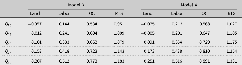
Notes: OC = Other costs, RTS = Returns to scale.
Appendix B: Estimates of Gradients for the Nonparametric Models
To examine the differences in the estimated elasticities and RTS with and without constraints in the nonparametric models (Models 1 and 2), we plot each of them in separate figures where the vertical (horizontal) axis measures objects of interest (elasticities and RTS) for the constrained (unconstrained) model. We draw a 45º line in each figure (Appendix, Figure 4 and Figure 5). Note that the observations will be on the 45º line if the measures of interest (elasticities or RTS) obtained from the constrained and unconstrained models are identical. Thus, a departure from the 45º line indicates differences in the estimated elasticities and RTS between the constrained and unconstrained models. Points below (above) the 45º line indicate that the measures from the unconstrained model are larger (smaller) than those obtained from the constrained model. Appendix Figure 4 plots the input elasticities and RTS for the standard case where the farmer uses observed output Y in the nonparametric models with and without constraints. The purpose of this plot is twofold. First, it is to investigate how close the estimates of different elasticities and RTS are from the constrained and unconstrained estimates for Models 1 and 2. Second, the plots will also reveal the negative input elasticities for the unconstrained Model 1. Figure 4 shows many negative elasticities obtained from Model 1. A plausible explanation could be the current lack of data on land quality, technology, and labor effectiveness in farm production. The negative values are also reflected in the RTS, which are negative for a few observations. Model 4 (Figure 4) imposes constraints that make the input elasticities nonnegative at each point. The figure reveals that the estimates, indicated by triangles, are close to the zero line. Thus, the estimates from the constrained and unconstrained models are identical. Consequently, there are no negative values for the RTS.

Figure 4. Restricted and unrestricted elasticity estimates for land, labor, other costs inputs, and RTS in Model 1.

Figure 5. Restricted and unrestricted elasticity estimates for land, labor, other costs inputs, and RTS in Model 2.
We perform a similar exercise in Appendix Table 5. In this case, Model 2, the output observed by the smallholder rice farmer is replaced with risk-adjusted output (CE output). The estimated elasticities for land, labor, other costs, and RTS are presented in Appendix Figure 5. Indeed, similarly to Appendix Figure 4, the unconstrained model shows some negative elasticities for land, labor, and other costs, and subsequently, the RTS estimates are negative. However, the negative elasticities are avoided in the constrained model (shown by triangles in Figure 5). Finally, Figures 4 and 5 show differences in the estimated elasticities between the constrained and unconstrained nonparametric models.


 Open access