


1. Introduction
The resource curse, though not without dissent, is a well-studied paradox. The resource curse theorizes that areas abundant in natural resources exhibit poor economic outcomes, including low levels of personal income, educational attainment, and other measures of well-being. The relationship between resource dependence and poverty includes theories related to human capital, industrial structure, and government power, among others (Douglas and Walker, Reference Douglas and Walker2017; Stedman, Parkins, and Beckley, Reference Stedman, Parkins and Beckley2009). Douglas and Walker note that these channels likely interact, and the boom and bust nature of resource-dependent economies also slows economic growth, which is itself most likely related to the various channels.
Scholars have long studied the resource curse in relation to oil-dependent economies (Humphreys, Sachs, and Stiglitz, Reference Humphreys, Sachs and Stiglitz2007). The advent of hydraulic fracturing and horizontal drilling represented a significant shift in resource extraction for regions dependent on oil and natural gas and in fact created new oil- and gas-dependent regions. The effects of these new extraction techniques renewed interest in the effects of drilling on economies and societies, with researchers studying effects on population (Measham and Fleming, Reference Measham and Fleming2014), employment (Tsvetkova and Partridge, Reference Tsvetkova and Partridge2016; Wrenn, Kelsey, and Jaenicke, Reference Wrenn, Kelsey and Jaenicke2015), income (Weinstein, Reference Weinstein2014; Weinstein, Partridge, and Tsvetkova, Reference Weinstein, Partridge and Tsvetkova2018), education (Cascio and Narayan, Reference Cascio and Narayan2015; Weber, Reference Weber2014), and other topics.
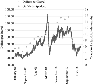
Texas oil fields have been at the center of many of these studies. Texas leads the United States in crude oil production, producing a fifth of U.S. oil (U.S. Energy Information Administration [USEIA], 2018). Driven by simultaneous advances in hydraulic fracturing and horizontal drilling, and soaring oil prices, crude oil production in Texas more than tripled between 2008 and 2014, according to the USEIA. Figure 1 depicts oil and gas prices over this boom and bust period.

Figure 1. Oil price versus Texas oil wells spudded, 2000–2017.
Perceptions about the permanence of local economic effects spurred considerable research around the United States related to the recent drilling boom. Is the resource curse relevant in the context of hydraulic fracturing and horizontal drilling? Has the nature or economic impact of some types of development changed? Are there other indirect effects on local educational attainment that may have negative consequences in the long run? If so, are there lessons communities can learn from this boom and bust cycle on how to maximize the benefits of future booms while preparing for inevitable busts?
These concerns motivate the intent of this article. In fact, there may be greater cause for concern in Texas because the United States’ leading oil producing state has below-average high school graduation rates (Stetser and Stillwell, Reference Stetser and Stillwell2014) yet has committed to an ambitious goal of increasing postsecondary attainment by more than 20% by 2030 (Texas Higher Education Coordinating Board, 2015). Because of lags in data availability and lifetime income effects not yet fully observed, we cannot yet investigate many of the questions on the permanence of income effects, but we can investigate indirect effects of the boom in terms of educational decisions that may have detrimental long-run effects over a worker’s lifetime. In particular, this article investigates the effect of the oil boom on local human capital investment, as proxied by educational attainment. First, has the latest oil boom led to a reduction in local high school graduation? Second, is this effect different for immigrants, a group that may be especially vulnerable to local wage effects? These research questions closely follow unanswered questions on the effects of busts that recent literature reviews suggest as an avenue for research (Fleming et al., Reference Fleming, Komarek, Partridge and Measham2015; Marchand and Weber, Reference Marchand and Weber2018). Although previous work has examined the effect of the shale drilling boom on the local overall completion or dropout in various regions (Cascio and Narayan, Reference Cascio and Narayan2015; Marchand and Weber, Reference Marchand and Weber2015; Rickman, Wang, and Winters, Reference Rickman, Wang and Winters2017), much of this research has not examined subgroup dropout rates. Among this article’s unique contributions are the following: (1) using previously unleveraged data on county-level graduation rates and accompanying drilling locations to directly examine the effect of local drilling, (2) examining the potential for heterogeneous effects on graduation rates among population subgroups, and (3) using spatial regression models to measure spillover effects in human capital investment and regional drilling activity. Following a literature review and data description, this article explores each research question. The last section contains implications of the findings for a variety of stakeholders.
2. Literature review
This article builds on a long line of research on the natural resource effects on local labor market conditions. Such research started with intercountry research, but then moved toward subnational variation, which allows for more credible empirical analyses by holding country-specific conditions constant (Marchand and Weber, Reference Marchand and Weber2018). Concurrent with these shifts in research, the widespread development of unconventional oil and gas resources in the United States fundamentally altered the energy industry and provided opportunities for new empirical work (Komarek, Reference Komarek2018; Kunce et al., Reference Kunce, Gerking, Morgan and Maddux2003; Weinstein, Reference Weinstein2014; White, Reference White2012).
This study focuses on local effects in Texas. Researchers have found significant and positive regional economic effects of the shale oil boom in Texas in the past. Lee (Reference Lee2015) summarizes and contributes to that regional economic research on effects in Texas. Lee’s (Reference Lee2015) (and other) research, however, does not investigate indirect effects, such as local graduation rates, that may have longer-term effects on local economic growth.
Temporal, spatial, and industrial impact variation deriving from the relatively new extraction techniques of horizontal drilling and hydraulic fracturing (which drove the oil boom) complicate empirical examinations of the effects of the recent oil boom. Spatial variation is particularly important because the oil and gas industries often rely on workers commuting long distances, especially in rural areas (Wrenn, Kelsey, and Jaenicke, Reference Wrenn, Kelsey and Jaenicke2015). The temporal issue is relevant, first, because direct labor demand from oil and gas extraction declines once wells start producing (Fleming et al., Reference Fleming, Komarek, Partridge and Measham2015) and, second, because as supply chains develop, they then may crowd out other types of economic activity (Tsvetkova and Partridge, Reference Tsvetkova and Partridge2016). Indeed, the drop in labor requirements between drilling and extraction is precipitous, with estimates ranging from 9 to 13 full-time equivalent (FTE) employees per well in the year of drilling and completion to 0.2–0.4 FTE employees per well in production (Kelsey, Partridge, and White, Reference Kelsey, Partridge and White2016). These numbers represent requirements for oil wells; gas wells have different FTE impacts and different extraction monitoring requirements, so the inclusion of both in estimates may bias results for Texas (Lee, Reference Lee2015). Furthermore, oil drilling represents the bulk of drilling and local impacts in Texas; as we noted previously, Texas leads the United States in crude oil production. Fleming et al. (Reference Fleming, Komarek, Partridge and Measham2015) note that higher spending in local areas may result from higher disposable income, generating spillovers into some nontraded sectors of a local economy, while oil and gas salaries are often higher than those offered by agriculture, manufacturing, or services, generating crowding-out effects on the traded sector. These high wages may also reduce incentives for local high school students to graduate.
Direct income effects generally come from either new and higher salaries related to the oil and gas industry or leases paid by the industry to landowners. Given that many rural areas also see local population decline, population effects are also of interest and are generally found to be positive (Measham and Fleming, Reference Measham and Fleming2014; Tsvetkova and Partridge, Reference Tsvetkova and Partridge2016), though there is also some evidence of limited or no population effects (Munasib and Rickman, Reference Munasib and Rickman2015). There is also some evidence of spillovers being short lived (Komarek, Reference Komarek2016).
Although short-term positive wage effects generally have a positive effect on the local economy in the short run, human capital effects of oil and gas drilling are also of interest, especially when examining the long-term effects of oil and gas drilling. Within the context of human capital, the long term may be a generation or more. The resource curse leads to a fear that oil and gas reduces the marginal benefit of education by increasing the number of high-pay, low-skill jobs, which reduces educational aspirations and, as a result, lifetime earnings. The natural resource curse has a long history of study internationally, with recent subnational work specific to the United States. Much of this research focuses on the links between natural resources and poverty, including links between schooling and poverty (Humphrey et al., Reference Humphrey, Berardi, Carroll, Fairfax, Fortmann, Geisler, Johnson and Summers1993). Humphrey and coauthors describe a “rational underinvestment” (p. 145) in human capital in response to perceived employer needs and educational payoffs. Freudenburg and Gramling’s (Reference Freudenburg and Gramling1994) analysis further explores themes from Humphrey et al., and Freudenburg and Gramling conclude that education may be an avenue for resource-depending regions and countries to avoid or move past the resource curse. Papyrakis and Gerlagh (Reference Papyrakis and Gerlagh2007), for example, show natural resource abundance decreases local schooling, which, among other channels, causes a negative effect of natural resource abundance on local growth. This local growth effect may then affect the prospects of the next generation. Johnson and Stallmann (Reference Johnson and Stallmann1994) describe the persistence of poverty in resource abundant areas as the result of rational decisions wherein individuals choose to forego education in response to relatively high wages for low-skilled resources work; however, low levels of education may depress wages and reduce employability across entire communities in a self-perpetuating cycle (Johnson and Stallmann, Reference Johnson and Stallmann1994; Leatherman and Marcouiller, Reference Leatherman and Marcouiller1996; Marshall et al., Reference Marshall, Fenton, Marshall and Sutton2007).
A wide body of literature explores the social and economic causes and effects of dropping out of high school. Finn’s (Reference Finn1989) models of high school dropout are seminal. Tinto’s (Reference Tinto1993) model describing the interactive causes of college dropout has been found applicable to the high school situation as well. These models consider student abilities, school characteristics and the student’s experience with the school, scholastic outcomes, and peer and family influences. The economics literature has taken a pragmatic approach associating dropouts with characteristics such as lower scholastic ability and motivation and comparative advantage in jobs not requiring a degree (Eckstein and Wolpin, Reference Eckstein and Wolpin1999), which can make dropping out a rational choice. However, students may also fail to perceive benefits from graduation, experience familial financial difficulties resulting in the need for employment, have a child on the way, see their peers dropping out, or leave school for a host of other reasons (Eckstein and Wolpin, Reference Eckstein and Wolpin1999; Kearney and Levine, Reference Kearney and Levine2014). Stetser and Stillwell (Reference Stetser and Stillwell2014) report lower graduation rates for black, Hispanic, and Native American students relative to their white counterparts. They found students with limited English proficiency had the lowest graduation rates at a mere 57%, while economically disadvantaged students and students with disabilities also had below-average graduation rates.
Several factors associated with high school dropouts are prevalent in regions with strong oil and gas extraction sectors, including relatively high wages for unskilled work, potential for income inequality and/or family financial distress as housing and other prices are driven up, and seeing peers enter the workforce. Although some families see windfall lease and royalty payments, those typically accrue to landowning residents (or formerly landowning residents who reserved mineral rights), increasing inequality. Some families also experience increased income through overall wage increases in active shale regions, but those same wages can attract potential dropouts. Though less work has examined the effect of the shale boom on local education levels, Weber (Reference Weber2014), using production data and educational attainment for the population aged 25 and older, looks at resident populations and finds that the shale boom did not erode local human capital stock in a four-state region in the southwestern United States, including Texas. Cascio and Narayan (Reference Cascio and Narayan2015) suggest Weber’s focus on workers over the age of 25 may reflect migration rather than educational decisions of young adults. They find that horizontal drilling and hydraulic fracturing generated higher high school dropout rates among young men, primarily by increasing the relative wages of men without a diploma. Similarly, Marchand and Weber (Reference Marchand and Weber2015) find that economically disadvantaged, English as a second language (ESL), and vocational students in areas of Texas with more shale resources were pulled out of schools and into the labor market during the 2000s. Measham and Fleming (Reference Measham and Fleming2014) find a positive effect insofar as they find fracking leads to higher proportions of youth aged 15–24 and 25–34 with university degrees and advanced technical qualifications compared with other rural regions in the short term. They do not show that this would be a permanent effect, rather than a “boom effect,” in which highly educated technical and engineering workers follow the initial drilling.
Using the synthetic control method, Rickman, Wang, and Winters (Reference Rickman, Wang and Winters2017), conversely, find significant reductions in high school and college attainment in Montana, North Dakota, and West Virginia because of the shale booms. Schafft et al. (Reference Schafft, Glenna, Green and Borlu2014) find some evidence of student turnover, perhaps because of transient worker families and displacement of lower-income families because of increased housing demand and prices. Marchand and Weber (Reference Marchand and Weber2015) look specifically at Texas schools, examining compositional effects, and find the shale boom areas (as measured by shale depth) are associated with decreasing populations of economically disadvantaged and ESL students, which they attribute in part to negative selection of these students into the low-skilled labor market. They also show that shale counties with increased tax revenues invested in capital, rather than teachers, resulting in no increases in student achievement. Their study uses school district and county-level data from 2000 to 2013 with shale depth as a proxy for shale oil and gas endowments. Specifically, the interaction between energy prices and shale depth is used as an instrument for the local wage. We use the more direct measure of oil spuds and examine immigrants, a subgroup excluded from their analysis.
Despite these limited and somewhat contradictory findings, there is limited other empirical evidence on the effects of the shale boom on local educational attainment. Further, the aforementioned human capital–focused studies miss the analyses of whether the shale boom has affected the real demand for education and how this demand varies by subgroup. Nevertheless, the literature within agricultural economics and related disciplines is clear that a well-educated workforce is critical to successful rural economic outcomes (Barefield, Reference Barefield2009; Partridge and Olfert, Reference Partridge and Olfert2011). This literature links education to economic outcomes for both individuals and community economies, and the immediate decision to drop out versus obtain a high school diploma or even continue to postsecondary college or vocational training is likely to have long-term effects on the earning potential of individuals and their families (Lleras, Reference Lleras2008; Torche, Reference Torche2015), as well as the economic success of communities and regions (Dudensing and Barkley, Reference Dudensing and Barkley2010). This article thus contributes evidence to the ongoing debate on the effects of the oil and gas boom on local educational attainment with the advantage of specific county-level panel data on oil spudsFootnote 1 and high school dropout rates, which year-to-year trends represent changing demand for education.
We first examine overall high school dropout rates and then investigate effects of drilling on student subgroups, including the immigrant subgroup, which may be more susceptible to local wage effects. Immigrant results may differ because the vast majority of immigrant children in the United States are Latino, and Latino high school children are disproportionately likely to need to work to support their family economically (Behnke, Gonzalez, and Cox, Reference Behnke, Gonzalez and Cox2010) and drop out of high school (Fischer, Reference Fischer2010). Previous research shows that there exist substantial differentials in graduation rates across subgroups. This article contributes to the current understanding of potential local resource curse effects by investigating the effects local fracking activity has on graduation rate overall and among a group that may be particularly vulnerable to the positive wage effects: immigrants. The results indicate that local oil drilling is associated with higher future dropout rates for local immigrant high school children.
3. Methods
3.1. Data
Our examination focuses on the state of Texas. Figure 2 presents a map of the counties and shale plays under consideration, overlaying the number of oil spuds in each county. The Permian Basin and the Eagle Ford represent the shale plays over which the most oil drilling has occurred in the time period under consideration (2010–2014). Figures 3 and 4 overlay the corresponding average county-level overall and immigrant dropout rates, respectively.

Figure 2. County map of Texas oil spuds with shale plays.

Figure 3. County map of Texas with average overall dropout rates, 2010–2014.

Figure 4. County map of Texas with average immigrant dropout rates, 2010–2014.
Our models use data from the U.S. Bureau of Economic Analysis (BEA). The BEA measures personal income by place of residence, emphasizing the need for the examination of potential spatial spillover effects to account for commuters. We measure the intensity of oil and gas extraction by the numbers of oil spuds, or newly completed oil wells.Footnote 2 The Texas Railroad Commission (TXRRC) provides data on the numbers of new and legacy oil and gas wells. Oil spuds capture the employment impacts of shale drilling because employment needs are significantly larger during the drilling phase than the production phase (Hartley et al., Reference Hartley, Medlock, Temzelides and Zhang2015). Table 1 presents summary statistics for employment, oil well counts, and other control variables (inclusion discussed subsequently) across the various shale formations in Texas, as well as the Texas averages.
Table 1. Summary statistics

Notes: ACS, American Communities Survey; BEA, Bureau of Economic Analysis; TEA, Texas Education Agency; TXRRC, Texas Railroad Commission.
The Texas Education Agency provides the data on county-level dropout rates and defines a dropout as follows: “A dropout is a student who is enrolled in public school in Grades 7-12, does not return to public school the following fall, is not expelled, and does not: graduate, receive a General Educational Development (GED) certificate, continue school outside the public school system, begin college, or die” (Murphy et al., Reference Murphy, Ryon, Traphagan and Wright2016, p. x). The Texas Education Agency does not include individuals who move out of state as dropouts, but rather, as students move out of state, they reduce the number of students enrolled (Murphy et al., Reference Murphy, Ryon, Traphagan and Wright2016). Using dropout rate as the dependent variable has the advantage of not being biased by changes in the total number of migrants in an area, because it measures the rate, rather than the count. Some disadvantages may be that the sensitivity of the dropout rate to additional student dropouts varies depending on the total number of students in that county, and the county-level dropout rate is created by dividing school districts that run across county lines, which is an inexact process.
Texas does now require students to be enrolled in school until age 19 (though the age was 18 until the 2015–2016 school year) unless they are working on a GED, have been expelled, or have graduated. Even after enacting this law, the state’s 2015–2016 longitudinal dropout rate (including dropouts over the 4 years since beginning grade 9) was 6.3% (Murphy et al., Reference Murphy, Ryon, Traphagan and Wright2016). Annual dropout rates, used in this study to better account for economic fluctuations, are smaller than longitudinal rates. Dropout rates are higher among students older than usual for their grade level, some minorities (e.g., African American and Hispanic), economically disadvantaged students, especially English language learners, immigrants, and students from migrant families.
The Texas Education Agency classifies an “immigrant” as a student who: “(1) is aged 3 through 21; (2) was not born in any state in the United States, Puerto Rico, or the District of Columbia; (3) has not been attending school in the United States for more than three full academic years. U.S. citizenship is not a factor when identifying a student as an immigrant for the purpose of public school data collection” (Murphy et al., Reference Murphy, Ryon, Traphagan and Wright2016, p. 41).
3.2. Modeling considerations
Recent literature on the shale oil and gas boom uses numerous different modeling techniques. This article takes advantage of those findings to inform the inclusion of various controls in our regression analysis. For example, it is essential to include year fixed effects (FEs) to control for oil and gas prices because incorporating changes in prices allows for a fuller explanation of the link between dependence and economic growth (Marchand and Weber, Reference Marchand and Weber2018). The current article examines substate variation, increasing credibility by holding state-specific conditions such as energy policy and oil taxation constant and focusing on localized differences potentially associated with oil and gas production. Because only Texas counties are included in this analysis, results may be specific to Texas, although expansion of the model to include other states could test the generalizability of the county-level results across states.
Although the regressions control for different county location over the different shale formations, they do not use location as the fundamental indicator of oil/gas effect because linking initial dependence on a particular resource to future economic growth is problematic as initial dependence itself may endogenously affect economic performance. Rather, we examine “oil spuds” as our indicators. Spuds indicate new activity, and with the advent of hydraulic fracturing, new wells were not conditioned on prior oil dependence. The number of annual spuds was greater in the newly accessible Eagle Ford shale, where growth outstripped most traditionally energy-dependent counties. For example, in our data set, Karnes County in the Eagle Ford shale had 130 spuds in 2010 and 370 in 2014, which led to an increase in producing oil wells from 135 in 2000 to 1,836 by 2016 (TXRRC, 2000, 2016). Both shale play location and oil spud numbers are imperfect indicators. Regardless, different shale playsFootnote 3 have different extraction and quality rates (Lee, Reference Lee2015), and the geography of the various shale plays may influence local conditions, so we include control variables for each of the five shale plays in Texas in our ordinary least squares (OLS) estimates. Furthermore, fixed geologic measures of resource quality could have different effects depending on other conditions such as changes in world energy market prices or new developments in oil drilling technology like ongoing improvements in hydraulic fracturing (Fleming et al., Reference Fleming, Komarek, Partridge and Measham2015).
Measuring employment is imperfect because broad measures of oil and gas industry activity from the BEA pick up oil and gas corporate administration employment and earnings, whereas this article is interested in the prevalence of low-skill labor that may incentivize dropouts. Our qualitative interest is in the economic effects where extraction occurs, rather than where oil-related firms are located. Further, much of the BEA data are place of residence data. This may be particularly important in the oil and gas extraction industry, in which long-distance commuting or fly-ins are frequent. Still, members of many oil field families follow boom activity, although families may trail, especially within a school year. Thus, residence-based data are preferable for this research because of the residential nature of students’ school enrollment. Further, firm-based data often do not fully represent the oil field location as large energy corporations are headquartered in permanent locations, such as Houston, while place of work data are suppressed to avoid disclosure at smaller geographies. Hence, research on the effects of oil drilling may understate local impacts because the share of workers officially residing near the drill site can be relatively low. To investigate the extent to which this is a concern, we include spatial spillover effects.
Using newly drilled wells as an indicator of extraction level prevents the limitation of including oil-related firms, but it is also imperfect as it is a noisy measure of oil and gas activity. Specifically, where and how much to drill may depend on important and hard-to-observe characteristics of the local economy and geography correlated with socioeconomic measures (Marchand and Weber, Reference Marchand and Weber2018). On the other hand, our data examine oil spuds, rather than existing well counts or existing well production levels. Oil spuds have the advantage of examining the impact of the shocks to the local economy when the employment effects would be the largest.
Weber (Reference Weber2012) and Fleming et al. (Reference Fleming, Komarek, Partridge and Measham2015) note that such counts of oil wells, the key explanatory variable, may be correlated with omitted variables that affect oil drilling activities as well as the local economy. Regressions excluding those confounding factors would result in biased estimates because of endogeneity in the explanatory variables. The control variables capture local socioeconomic, labor market, economic, and geographic characteristics that likely correlate with the number of oil wells and local economic growth. For the purposes of this article, controlling for an area’s initial level of educational attainment is essential, and hence, the regressions control for the share of the county population with a bachelor’s degree. The structure of the local economy is particularly important, given various concerns of inverse impacts in the tradable and nontradable sectors. Our regression controls for the structure of the local economy by including the shares of total income earnings in the agricultural, construction, manufacturing, and retail industries. Initial per capita income and employment are the convergence variables (Barro, Reference Barro1998; Barro and Sala-i-Martin, Reference Barro and Sala-i-Martin1992). Although a difference-in-difference approach may be preferable, given different (or microlevel) data, the data that we have from 2010 to 2014 do not contain a clear start date for the drilling, nor a clear treatment group, in which select counties would be consistently exposed to high levels of oil spuds after a treatment start date. Although we could specify some counties with relatively high oil spuds in our time period and indeed find significant effects of drilling on immigrant dropout rate in some of those specifications, selection of the threshold for inclusion in the treatment group is necessarily arbitrary. Therefore, we believe the subsequent regression represents the best approach, given the limitations of available data.
We control for population density, urban adjacency, and rurality with the U.S. Department of Agriculture’s (USDA) Rural-Urban Continuum Codes to account for how energy lease prices and labor market elasticity may vary nonlinearly over the rural-urban spectrum.Footnote 4 Finally, we also include the foreign-born population. Although the use of dropout rate prevents higher concentrations of immigrants from influencing results, it may be that higher local wages attract a type of immigrant whose children are more likely to drop out. To help control for this possibility, we include the local foreign-born population. A more direct measure would be the immigrant student population, but the Texas Education Agency does not release exact counts of immigrant students to prevent disclosure of personal identifiable information.
Thus, the FEs regression equation can be stated as
 $$ \Delta {y_{it}} = \delta {s_{it}} + \beta {X_{it}} + {\alpha _i} + {\gamma _t} + {\mu _{it}}, $$(1)
where sit is the number of oil spuds in county i in year t, αi is the county FE, γt is the year FE, and Xit is a vector of the other control variables, which include county population, the share of the population that is black, the share of the population that is Asian, the share of the population that is Hispanic, the share of the population that is foreign born, the share of the population that has a bachelor’s degree, and the share of local earning by farming, construction, manufacturing, or retail earnings. Our pooled OLS regression of course drops the county FE, but also includes shale play FEs and USDA Rural-Urban Continuum Code FEs in Xit.
4. Results
This article begins its analysis with some classic panel regression techniques including pooled OLS and FEs. For ease of interpretation, the dependent and independent variables are standardized. With the Hausman test indicating significance of time-invariant FEs, the FE regression accounts for these characteristics to the extent to which they are time invariant, while the pooled OLS regression controls for these characteristics by including other geographic controls including the shale play FE and the USDA Rural-Urban Continuum Codes.Footnote 5 That the specification maintains the base levels of the explanatory variables, while using the future growth in the dropout rate as the dependent variable, also lessens concerns of endogeneity. This so-called weakly exogenous approach assumes that future growth rates of our dependent variables do not affect current levels of explanatory variables and is common in regional growth literature (Levine, Loayza, and Beck, Reference Levine, Loayza and Beck2000). Note also that the dropout rates follow the academic calendar, so the model lags the explanatory variables by half of a year (e.g., the model regresses dropout rate growth between the 2011–2012 and 2012–2013 academic years on the 2011 base level of oil spuds).
Using the aforementioned control variables, Table 2 presents the regression results when regressing the dropout rate growth on base levels of the explanatory variables. Columns (1) and (2) present the results with the 1-year growth in the overall dropout rate as the dependent variable, while columns (3) and (4) present the results with immigrant dropout rate as the dependent variable.
Table 2. Panel regression results: standardized growth in dropout rate, 2010–2014

Notes: Robust standard errors in parentheses. FE, fixed effect; POLS, pooled ordinary least squares; RUCC, Rural-Urban Continuum Codes; USDA, U.S. Department of Agriculture. ***P < 0.01, **P < 0.05, *P < 0.1.
Though the panel regressions fail to find statistically significant evidence of a relationship between the number of local oil spuds and the overall dropout rate, there is evidence of a positive effect on the number of local oil spuds and the local immigrant dropout rate. These results are consistent with Weber (Reference Weber2014) for the overall student population in the Southwest and with Marchand and Weber (Reference Marchand and Weber2015) for the economically disadvantaged, English language learners, and vocational education students in Texas, at least to the extent one might expect immigrant students to fall into these categories. A high correlation between students in these groups seems likely. Specifically, the pooled OLS and FE regressions indicate that a 1 standard deviation increase in the number of oil spuds (74.44 oil spuds) implies the immigrant dropout rate will increase by 0.08 and 0.40 standard deviations (growth of 0.49% and 2.47%), respectively.
Finally, investigating the reason why immigrant children may differ from the general population is of interest. There is a body of education literature indicating that high student mobility increases the risk of dropping out of high school (Rumberger and Larson, Reference Rumberger and Larson1998; Stiefel, Schwartz, and Conger, Reference Stiefel, Schwartz and Conger2010). Hence, it may be that immigrant children are more mobile and thus already more likely to drop out. Consistent with Marchand and Weber (Reference Marchand and Weber2015), these students may struggle to learn English and perform well at school, and they might be economically disadvantaged. It may be that immigrant children are more susceptible to dropping out in favor of high-paying local jobs. Indeed, immigrant results may differ because immigrant children in the United States are disproportionately likely to be Latino, and Latino high school children are disproportionately likely to need to work to support their family economically (Behnke et al., Reference Behnke, Gonzalez and Cox2010) and drop out of high school (Fischer, Reference Fischer2010). In the terminology of Humphrey et al. (Reference Humphrey, Berardi, Carroll, Fairfax, Fortmann, Geisler, Johnson and Summers1993), these students may engage in “rational underinvestment” in education. Table A1 in the Appendix related the same set of control variables, but with the dependent variable as the (county-level) log of wage. Though the FEs regression finds a statistically insignificant relationship, the OLS shows the expected relationship: growth in local oil drilling activity has a positive effect on local wages.Footnote 6 Thus, in order to further investigate the connection between immigrant dropout rates and drilling activity, we also regress HispanicFootnote 7 and economically disadvantagedFootnote 8 dropout rates on oil spuds.
Table 3 shows that oil spuds have a statistically insignificant effect on the dropout rate for both Hispanic and economically disadvantaged children. Unfortunately, more specific breakdowns, for example “Hispanic immigrants” are not currently available from the Texas Education Agency. Regardless, the insignificant results may indicate that the effects on immigrant dropout rates are not solely attributable to immigrants being more likely to be Hispanic or to being economically disadvantaged.
Table 3. Panel regression results: standardized growth in dropout rate, 2010–2014

Notes: Robust standard errors in parentheses. FE, fixed effect; POLS, pooled ordinary least squares; RUCC, Rural-Urban Continuum Codes; USDA, U.S. Department of Agriculture. ***P < 0.01, **P < 0.05, *P < 0.1.
Recent econometric work examining the effects of oil and gas extraction examines the importance of spatial spillover effects (Lee, Reference Lee2015; Weber, Reference Weber2014). Hartley et al. (Reference Hartley, Medlock, Temzelides and Zhang2015), for example, found that spatial correlation accounts for 17% of the total employment effect of gas drilling activity, indicating that other spillover effects on increasing dropout rates may follow.Footnote 9 In simple terms, an oil spud may locate near a county line, and county lines are arbitrary political boundaries, rather than economic boundaries, so the effects of that oil spud would spillover to neighboring counties. Thus, regressions that omit that spillover effect may represent biased estimates of the relationship between local drilling and dropouts by ignoring neighboring county dropouts. Beyond empirical considerations, using a spatial panel model also quantifies local versus neighboring effects of oil and gas drilling. Further, if limited local hiring by oil and gas companies mitigates the local effects, spillover effects are also of qualitative interest. The relationship between oil spuds and overall, Hispanic, and economically disadvantaged dropout rates remains insignificant, so this section focuses on a spatial panel regression examining the effect on immigrant dropout rates.
Spatial spillovers in the dependent variables are also of concern. Schafer and Hori (Reference Schafer and Hori2006) show school processes, administration, effectiveness, and structure all influence high school dropout rates and are often spatially related. They emphasize that these mechanisms driving dropout extend beyond the school level and may thus cross county lines. Given our data are at the county level, school districts crossing into multiple counties might exacerbate this effect. Failure to control for how these other factors influence regional dropout rates may result in biased estimates because they attribute the effect of regional clustering in dropout rates to neighboring drilling.
Following LeSage and Pace (Reference LeSage and Pace2009) and Elhorst (Reference Elhorst2010), we first estimate the more general FEs spatial Durbin model, given in equation (2), so that we can test the restrictions imposed by nested models, and also for a significant effect of neighboring counties’ drilling on dropout rates. We use a queen contiguity spatial weighting matrix.Footnote 10 Then, we test the restrictions imposed by the spatial autoregressive (SAR) model and spatial error model (SEM). Specifically, if θ = 0 and ρ ≠ 0, the model collapses to SAR, whereas if θ = –βρ, then the model is an SEM. With a χ 2(9, n = 1016) = 10.57, we fail to reject that θ = 0, and we can reject with 90% confidence that ρ = 0. These results indicate that there is spatial dependence in the dependent variable but not the explanatory variables.
Finally, we must use information criteria to test FEs SAR, given in equation (3), against FEs SAC (SAR with spatially autocorrelated errors), given in equation (4), because they are nonnested.
 $$ \Delta {y_{it}} = \rho W\Delta {y_{it}} + \beta {X_{it}} + \theta W{X_{it}} + {\alpha _i} + {\gamma _t} + {u_{it}} $$(2)
 $$ \Delta {y_{it}} = \rho W\Delta {y_{it}} + \beta {X_{it}} + {\alpha _i} + {\gamma _t} + {u_{it}} $$(3)
 $$ \Delta {y_{it}} = \rho W\Delta {y_{it}} + \beta {X_{it}} + {\alpha _i} + {\gamma _t} + {v_{it}}$$(4)
 $${v_{it}} = \lambda W{v_{it}} + {u_{it}}$$
The information criteria comparison is mixed, though similar, indicating a small preference toward SAC with the log likelihood.Footnote 11 We focus on the SAC results here, though the results of the two models are quantitatively and qualitatively similar. For all of these estimators, we use the suggested maximum likelihood estimator, which is consistent and asymptotically efficient (Ward and Gleditsch, Reference Ward and Gleditsch2008).
Table 4 provides coefficient estimates, but as the spatial lag of the dependent variable is included in the model, these coefficient estimates (including the spatial lag of dropout rates) lose their conventional interpretation as marginal effects because the spatial lag gives rise to a series of feedback loops and spillover effects across regions. Therefore, we also calculate the average direct effect, average indirect (spillover) effect, and average total effect, all of which have the conventional (marginal effect) interpretation in their respective directions (LeSage and Pace, Reference LeSage and Pace2009). Table 3 indicates that the FE results are generally the same as the direct effect estimated in the FEs SAC, but with the indirect effect, the total marginal effect increases to about 0.60 from 0.40. Thus, spillover effects to adjacent counties may increase total effects. This is consistent with regional effects on wages and with administrative impacts in school districting. Although the findings indicate no statistically significant indirect effect on dropout rates, they also indicate that a 1 standard deviation increase in the number of county oil spuds (74.44 oil spuds) implies the county immigrant dropout rate will increase by between 0.08 and 0.60 standard deviations (0.49% and 3.71%). Given that in 2014 the average number of immigrant students in a Texas county is about 106.23, this finding implies that our estimate of the effects of an increase in the number of oil spuds in a county by 1 standard deviation increases to 1 and 4 immigrant student dropouts annually, on average. Of course, in counties with a higher number of immigrants, this effect would be substantial.
Table 4. Fixed effects SAC model: standardized growth in immigrant dropout rate, 2010–2014

Notes: Robust standard errors in parentheses. FE, fixed effect; SAC, spatial autoregressive with spatially autocorrelated errors. ***P < 0.01, **P < 0.05, *P < 0.1.
5. Conclusions
This study considers the effects of county-level oil drilling activity on local high school dropout rates in Texas. We do not find evidence that the latest oil boom led to a reduction in local high school graduation rates for the general population, which is consistent with Weber’s (Reference Weber2014) finding that the shale boom did not affect human capital accumulation of the population aged 25 and older. However, we do show that immigrant dropout rates increase in the presence of local oil drilling. On this second question, we extend previous findings that high student mobility increases the risk of dropping out of high school (Rumberger and Larson, Reference Rumberger and Larson1998; Stiefel et al., Reference Stiefel, Schwartz and Conger2010). It may be that immigrant children are more mobile and thus already more likely to drop out. Still, our models are able to detect a relationship between oil spuds and immigrant dropout rates, whereas they do not find a statistically significant relationship with overall dropout rates. Regardless, this article provides evidence that though the resource curse’s negative effects on human capital accumulation may be difficult to detect for the general population, local resource extraction appears to have a negative effect on human capital for the immigrant population.
Our finding that local oil drilling increases immigrant dropout rates is directionally consistent with Marchand and Weber’s (Reference Marchand and Weber2015) finding that economically disadvantaged, vocational, and ESL students in Texas were more likely to leave school during the oil boom. Their approach of instrumenting log(wage) with shale depth makes a magnitude comparison difficult. However, we do not find significant changes in the overall dropout rate for all students. Although our results differ from those of Cascio and Narayan (Reference Cascio and Narayan2015), those authors found greater significance and magnitude prior to 2012 and posit that the wage premium for dropouts had eroded in later years. These results are potentially consistent with Weber’s (Reference Weber2014) finding that adult education levels are not diminished by the oil boom in the U.S. Southwest. Across the population, increases in dropout rates among immigrants may be canceled out by increased education in other populations (e.g., females and students benefiting from increased familial incomes). Furthermore, the significant spatial dependence in dropout rates may be indicative of the regional (cross-county) effects in dropout rates. Future research could examine whether these regional effects are because of adjacent job availability or regional wage inflation resulting from the oil drilling, or simply the school processes, administration, effectiveness, and school district structure that we discussed previously.
It is tempting to think a student might drop out to work a few years and take advantage of a temporary lucrative opportunity, which then funds a GED degree and subsequent college education after the boom. Perhaps the student learns the value of an education through performing hard physical labor or sees an opportunity to advance within his current company by completing an education. Generally, this view is overly optimistic, particularly for Hispanic high school dropouts, who are more likely to be immigrants, with just 9% Hispanic high school dropouts earning a GED credential and just 40% of those with a GED pursuing additional education (Fry, Reference Fry2010). Hispanic dropouts fare worse than other ethnic groups in this regard; for example, about 20% of black high school dropouts and 30% of white high school dropouts have a GED.
Furthermore, the long-term economic consequences of dropping out of high school are significant. Indeed, Hispanic adults with a GED had a 2 percentage point higher unemployment rate than Hispanic adults with a high school diploma (Fry, Reference Fry2010). Although the possibility of dropouts saving for college exists, the authors note that the percent of individuals pursuing this route is undoubtedly small. Given the potential long-term negative effects of reduced human capital investment, this article’s findings corroborate the importance of completing a high school education. The propensity of immigrant students to drop out may be altered by policy and educational interventions. Although a potential topic for future research, the economic and social motivations for dropping out may be similar for students from mining and agricultural migrant families. To prepare for the higher needs of migrantFootnote 12 children, many public Texas schools require parents to fill out paperwork certifying that they are (or are not) migrant farmworkers. Perhaps similar efforts should be made with migrant oil field workers; at least schools would be made more aware of these students’ migrant status and unique needs.
On the other hand, that the overall high school dropout rate is insignificant may indicate that other subgroups see a decrease in dropout rate from local oil drilling and the resultant higher wages. Though perhaps counterintuitive, given the reasoning in this article, it may be that certain subgroups benefit from increased parental income related to higher local wages, while experiencing less or limited pull themselves to those jobs. For example, it may be that women are less likely to work in oil drilling and receive the benefit of higher parental income, and thus experience less of the pressure to drop out for one of those jobs themselves (Cascio and Narayan, Reference Cascio and Narayan2015). Although testing of the effect of local oil spuds on female dropout rates indicates an insignificant effect, it may be that using more specific geography reveals this or other effects. Further delineating and examining subgroup dropout rates under finer geographic resolutions (given data availability) is an area for future research.
Taken together, our findings for the overall student body and for immigrants suggest that students and families with different socioeconomic characteristics may make different rational decisions about economic prospects from education versus immediate entry to the workforce. Both Johnson and Stallmann (Reference Johnson and Stallmann1994) and Freudenburg and Gramling (Reference Freudenburg and Gramling1994) recognize the role that individuals play in identifying their own prospects based in part on past experience. Our findings support Johnson and Stallmann’s call for rural youth to be better educated in the opportunities afforded them outside their current local economy, in an attempt to give them a broader experience set. In fact, given that a subset of minors make different choices, our results hint at a need for family education about an expanded opportunity set.
Finally, this article does not show that immigrant high school students are necessarily dropping out of high school to go work in local oil drilling jobs. Though the oil drilling jobs themselves may contribute to the dropout rate, this research cannot separate this direct effect and the indirect effect of those high-paying jobs causing a general wage increase locally. Finding a plausible mechanism to decompose these effects is also an area for future research. Still, given that Texas has set a target of 60% of adults ages 25–34 with a postsecondary certificate or degree by 2030 (more than 20% above current levels), dropouts pose a hurdle to the state’s economic competitiveness (Texas Higher Education Coordinating Board, 2015). Reducing dropouts and improving postsecondary enrollment and success, especially among the state’s economically disadvantaged and minority populations, including immigrants, will be an important area of future research.
Author ORCIDs
Craig W. Carpenter 0000-0001-7511-1168
Acknowledgements
The authors thank the editors and anonymous reviewers for their helpful and insightful comments that greatly improved this work. The authors are also grateful to Jim Lee for providing data on the quantity of oil wells in Texas and to the Extension-participating community members that motivated the analysis herein.
Appendix
Table A1. Relating oil well drilling to local wage growth, 2010–2014

Notes: Robust standard errors in parentheses. FE, fixed effect; POLS, pooled ordinary least squares; RUCC, Rural-Urban Continuum Codes; USDA, U.S. Department of Agriculture. ***P < 0.01, **P < 0.05, *P < 0.1.


 Open access