


Introduction
Accurate and up-to-date information on agricultural land use is essential to improve land management and food production, as well as to control the impacts of farming on the environment. Crop area extent estimates and crop type maps are considered crucial information in agriculture (Inglada et al., Reference Inglada2016). These data are equally useful for farmers’ associations, local land use planners and regional and governmental agencies, as well as for industrial food groups, and were requested for the specific case of the tomato crop by the Italian Association of Industrial Food Preserve (ANICAV) for the year 2016.
An example of a crop type for which timely information is especially valuable is tomato (Solanum lycopersicum). During the spring and summer seasons, central and southern Italian regions are concerned with activities related to industrial tomato horticulture. At the beginning of the crop season, farmers’ associations and organizations require estimates about the tomatoes that will be produced, which are presently derived from annual voluntary reports on areas with transplanted tomatoes submitted by farmers. The total tomato cultivation area is variable, due to seasonal and annual turnover of cultivation, and it is also influenced by spring commercial agreements between the production and the agro-industrial sectors. The amount of planted tomato can be used by producer associations to receive economic support from governmental agencies; precise tomato estimates allow improvements in the organization of the industrial transformation cycle; early data on tomato production may stabilize the market price, as uncertainty about expected production may cause speculation. The extent of tomato cultivation areas, as well as of other seasonal crops, is traditionally obtained through field assessments conducted by local agents; these data are limited and cannot be used to produce accurate estimates.
Remote sensing supports agricultural monitoring in different ways: hyperspectral and multispectral very high spatial resolution data are preferred, thanks to their ability to detect differences in reflectance found among crops, vegetation growing stages or health conditions. Examples range from the classification of different crops (De Wit and Clevers, Reference De Wit and Clevers2004; Fisette et al., Reference Fisette and Werle2005; Turker and Arikan, Reference Turker and Arikan2005; Conrad et al., Reference Conrad2010; Förster et al., Reference Förster2012; Inglada et al., Reference Inglada2015), to the detection of crop diseases (Hillnhütter et al., Reference Hillnhütter2011; Mahlein et al., Reference Mahlein2012), the assessment of health and support to precision farming (Seelan et al., Reference Seelan2003; Zhang et al., Reference Zhang2003; Pan et al., Reference Pan2015) and to estimates of productivity (Mosleh et al., Reference Mosleh, Hassan and Chowdhury2015; Geipel et al., Reference Geipel2016). Integration of multispectral and Synthetic Aperture Radar (SAR) data was also experimented with successfully in crop mapping research by Forkuor et al. (Reference Forkuor2014) and Inglada et al. (Reference Inglada2016).
Remote sensing provides data needed in horticulture (Usha and Singh, Reference Usha and Singh2013). Tomato mapping has previously been conducted successfully, but with data at a very high resolution: by Ozdarici-Ok et al. (Reference Ozdarici-Ok, Ok and Schindler2015) using single multispectral satellite images with spatial resolution <4 m, and by Senthilnath et al. (Reference Senthilnath2016) using Unmanned Aerial Vehicle (UAV) data. Other tomato-specific studies include the detection of stress induced by late blight disease using hyperspectral data by Zhang et al. (Reference Zhang2003), the correlation between vegetation indices and tomato yield, together with an analysis of spatial crop variability, done with proximal sensing by Marino and Alvino (Reference Marino and Alvino2014) and ground-based tomato remote sensing carried out by Mastrorilli et al. (Reference Mastrorilli2010) to evaluate crop water status dynamics. With on-demand airborne surveys, the ability to choose different on-board sensors allows specific data requirements to be met, in terms of spatial and spectral resolutions. Airborne surveys are an excellent option when resources are available, but the high data acquisition and processing costs, as well as the limited area coverage, hamper their operational and routine use in agriculture monitoring.
Among satellite platforms, hyperspectral sensors are best suited for crop characterization (Thenkabail et al., Reference Thenkabail2013) and provide better results than multispectral ones for single crop monitoring (Mariotto et al., Reference Mariotto2013). However, the current absence of hyperspectral satellite data, and the high costs associated with hyperspectral airborne surveys, limits their applicability. Advancements in spatial and spectral resolutions of recent multispectral sensors, together with the large area covered by a satellite image and the possibility of close multitemporal acquisitions, allow new possibilities in crop monitoring. For instance, the RapidEye sensor has been used frequently and successfully in agricultural monitoring, thanks also to the availability of a red-edge band, which allows discrimination of very fine differences in the reflectance of vegetation (Conrad et al., Reference Conrad2014; Shang et al., Reference Shang2014; Gerstmann et al., Reference Gerstmann, Möller and Gläßer2016). Satellite data at a very high resolution are available through commercial services that perform on-demand acquisitions, but their high cost limits an operational use in crop monitoring.
The advent of an open data satellite mission specifically tailored to agricultural monitoring, such as Sentinel 2 (S2) by the European Space Agency (ESA), broadens the opportunities of agricultural monitoring (Drusch et al., Reference Drusch2012; Immitzer et al., Reference Immitzer, Vuolo and Atzberger2016). At full operability, S2 has a 2–5 day revisiting time according to latitude, an enhanced spectral resolution with 13 bands from 490 to 2190 nm, and a spatial resolution variable between 10 and 60 m according to the band.
Considering the very high resolution needed to cope with the limited extent of tomato fields, the variability in transplanting dates in Italy, as well as the spectral similarity of tomato with other vegetable crops, tomato mapping at an early crop development stage can be considered a challenging task, unless very-high-resolution data from optimal dates are used. Tomato information is requested by users very early in the cropping season, when crops are not yet mature and discrimination from other crops is difficult; with the limited time between transplanting dates and early estimate requests, the availability of cloud-free satellite images is also reduced.
The current study documents the results obtained for early tomato field detection and mapping using data from ground surveys, airborne data and remote-sensing imagery, in seven areas previously identified in Central and Southern Italy. Additionally, an analysis of damage caused by a hailstorm during the growing season in one sub-area was also carried out. The main questions were related to the suitability of S2 to estimate tomato accurately at an early stage of crop development, and to identify abrupt growth changes in this crop.
Materials and methods
Study areas
The seven study areas (Fig. 1) are located in four Italian regions. The areas are characterized by different climatic conditions (temperature, precipitation), soils (according to pedo-climatic characteristics) and by variable transplanting dates, according to the seasonal climate and farming habits. Usually, transplants occur from the beginning of April to mid-June, with earlier dates in southern areas. Tomato is cultivated annually and has a life cycle of approximately 100 days; seeds are planted in greenhouses, seedlings are then transplanted and take about 20–30 days to cover the soil.
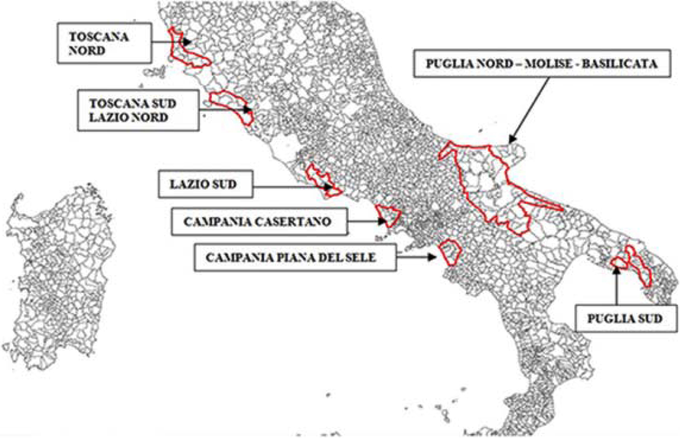
Fig. 1. The tomato study areas: Toscana nord (TN); Toscana sud–Lazio nord (TL); Lazio sud (LS); Campania Casertano (CC); Campania Piana del Sele (CPS); Puglia nord, Molise, Basilicata (PMB); Puglia sud (PS).
In three of the seven areas, an early estimate of tomato-planted surface (TS) was obtained by the first half of June: Campania Piana del Sele (CPS), Puglia nord–Molise–Basilicata (PMB) and Campania Casertano (CC), the areas responsible for most of the production. Tomato field maps were realized by 30 June in 2016 in all the areas.
Ground data
Extensive ground data surveys were carried out in the study areas between May and early June 2016 with the aim of providing ground truthing for satellite data classification, collecting information for all the different crop types occurring. To exclude non-agricultural zones inside the study areas, Corine Land Cover (CLC) 2012 IV level and thematic data extracted from OpenStreetMap (OSM) and Google Earth were used; the latter two include linear features such as narrow roads, railways, water courses and agricultural service areas. All the non-agricultural zones were masked out to produce the effectively cultivated agricultural surface (Table 1), which was used in subsequent analysis.
Table 1. Agriculture surface, tomato surface and ground observations per study area in 2015 and 2016, from north to south

Previously prepared Geographical Information System (GIS) layers, including roads and cadastral maps (‘cadastre’ is a technical term for a set of records showing the extent, value and ownership (or other basis for use or occupancy) of land) were uploaded onto laptops (Fig. 2), to allow visualization of the information collected during field operations. Local roads were treated as transects for collecting observations; these transects were selected randomly in a number sufficient to homogeneously cover each area. Crop information (geolocation, crop type, growing stage identified as initial, intermediate or full development of plants) was recorded at points along the transects spaced at least 900 m apart, for crops occurring on both sides of the road. Considering the limits in field survey design, imposed by private property and accessibility problems, this strategy was selected to ensure as much random observation of different crop types as possible. The number of observed crops per area is reported in Table 1.
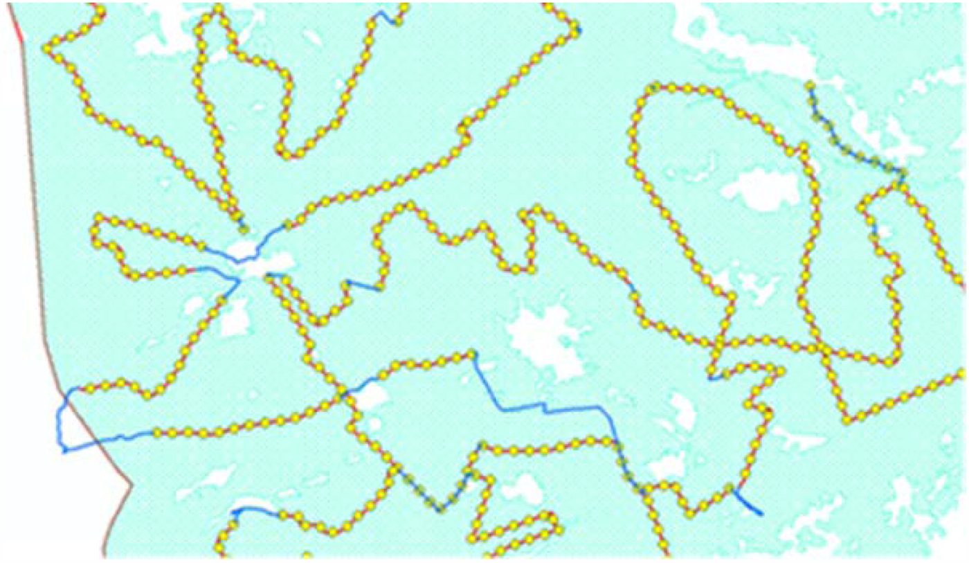
Fig. 2. Detail of a layer supporting the field work in Campania Casertano (CC) area: in light blue the agriculture areas, in white the masked areas, in red the transects, in yellow the established observation points, in blue the connection roads among transects.
The minimum number of crops per area, and therefore of points and transects to survey, was established prior to field operations, with the objective to collect information for >2% of the cultivated surface in each area. However, the mean size of fields is different in each area, according to topography, urbanization, agricultural practices and other local factors. A preliminary analysis of the cadastral maps allowed calculation of the mean size of agricultural fields in each area (approximately 2–4 ha). On the basis of the mean field size per area, the number of crops for which data had to be collected was established for each area to survey >2% of the cultivated surface. This by-area stratified random sampling approach was selected considering the main aim of tomato detection, the inaccessibility of certain zones, the need of collecting ground truthing homogeneously over the areas of interest and the uneven distribution of certain crop types. A minimum of 25 validation samples per crop type was required for these infrequent crop types.
Subsequently to ground truth data collection, polygons for the identified crop types were delineated on satellite imagery. Pixels included in these polygons were extracted and used as ground truth (training and validation) in the classification process, after excluding a buffer (internally and externally to the field perimeter) to minimize inclusion of non-cultivated pixels or pixels from adjacent non-identified crops.
A second ground truth survey was performed in late June 2016 in study area CC over 599 fields, using the previously described procedure. This second ground survey, carried out after the aerial survey in mid-June, was done to refine the tomato classification by means of aerial data photointerpretation; it targeted fields not used for satellite data training and validation and aimed to evaluate the improvement in accuracy of tomato maps after refinement based on photointerpretation.
Remote-sensing data
In four of the study areas, namely Toscana nord (TN), CC, CPS and PMB (Fig. 3), an aerial survey was conducted between 10 and 22 June in 2016 using a Sky Arrow 650 TC/TCNS aircraft equipped with the Terrasystem DFR system (http://www.terrasystem.it/en/dfr.htm), a modular system dedicated to agricultural monitoring. For the current study, the instruments included were: a multispectral four Charged-Coupled Device (CCD) camera in the visible to near-infrared (NIR) spectral range, a Hasselblad H3dII-31 digital camera, an Ashtech DG14 and Novatel OEM4 global positioning system (GPS) unit and a Systron Donner C MIGITS III INS/GPS unit. All the sensors were integrated in a single and flexible acquisition system, the parameters of which can be configured according to acquisition needs. Data acquisition software allowed simultaneous recording of different data and the position and asset of the aircraft, and association with the acquired imagery. Synchronization among GPS and sensors was managed by trigger transistor-transistor logic signals. The strips of aerial data were acquired along pre-established transects at 1675 m above ground level, with 0.60 longitudinal overlap and 0.20 lateral overlap. The following bands were acquired: red (R; centred at 680 nm), green (G; centred at 550 nm) and blue (B; centred at 500 nm) at 0.3 m; and the same R and G bands plus NIR (centred at 780 nm) bands at 0.8 m spatial resolution, all bands having 20 nm band width (Fig. 4). Raw aerial images were converted to standard image format using Hasselblad Phocus 2.5.2 software and then linked visually to ortho-corrected satellite imagery using the flight plan and the log data recorded during the aerial survey.

Fig. 3. Example of the aerial survey data strips over Campania Casertano (CC), Campania Piana del Sele (CPS) and Puglia nord, Molise, Basilicata (PMB) areas.

Fig. 4. (a) A false colour composite made by aerial data in red, green and near-infrared bands at 0.8 m; (b) a real colour image made by aerial data in red, green, blue bands at 0.3 m spatial resolution. Images are from Puglia nord, Molise, Basilicata (PMB) area, and show general agriculture fields.
A total of six S2 mostly cloud-free images were acquired to cover the study areas (Fig. 5, Table 2) and processed in the ESA Sentinal Application Platform (SNAP) tool to obtain orthorectified and atmospherically corrected imagery, with ten bands at 10 and 20 m spatial resolution in the visible shortwave infrared spectral range, including two bands at the red edge. Images were masked out for cloud presence and to retain only the cultivated surfaces. All bands were resampled to 10 m spatial resolution using the nearest neighbour procedure, and the normalized difference vegetation index (NDVI; Rouse et al., Reference Rouse, Freden, Mercanti and Becker1974) and red edge NDVI (Sims and Gamon Reference Sims and Gamon2002) computed, being the indices that preliminary crop separability analysis indicated as most relevant for crop discrimination. In classification, stacked bands and the two vegetation indices were tested as input to the classification algorithm, separately and together.
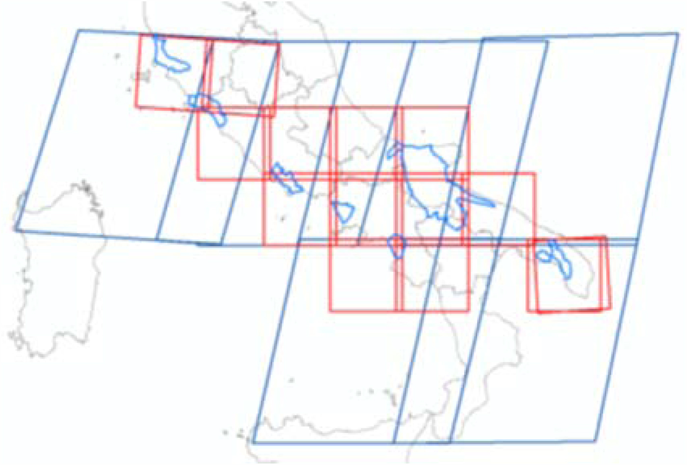
Fig. 5. Sentinel 2 footprints covering the study areas (in blue). Each S2 image is divided into granules (in red) according to the Universal Transverse Mercator (UTM) grid.
Table 2. Sentinel 2 imagery

Study areas: TN, Toscana nord; TL, Toscana sud–Lazio nord; LS, Lazio sud; CC, Campania casertano; CPS, Campania Piana del Sele; PMB, Puglia nord, Molise, Basilicata; PS, Puglia sud.
To evaluate the S2-based statistics of tomato growth (TG) in a hailstorm-affected area, a RapidEye image (five spectral bands including R, G, B, red edge and NIR, at 5 m spatial resolution) dated 17 June 2016 was also employed.
Data analysis
The first activity was the very early estimate of tomato-cultivated surface based on quantitative ground data: this is a numerical estimate, producing timely information on the number of hectares planted with tomato, conducted when the development of plants is too limited to allow remote-sensing use.
For the first activity, the TS was calculated in each study area according to the following formula:
 $${\rm TS} = p \times {\rm TA}/c$$
where p is the tomato frequency among crops observed in the ground survey, TA is the cultivated surface and c is a correction factor equal to the mean of the ratio between early estimated tomato surface and final mapped tomato surface as recorded in previous years (2013 and 2014, unpublished data from Associazione Nazionale Industriali Conserve Alimentari Vegetali (ANICAV)). Coefficient c was introduced to compensate for the error caused by annual variability in sample distribution, tomato field size, TA and TS. Until now, only 2 years were available for c calculation; however, the factor was introduced in view of future tomato estimates. It is area-specific and ranged between 0.97 and 1.58.
The second activity was tomato mapping at the beginning of crop season based on S2 stacked bands and vegetation indices, used separately or together as input in the classification algorithm. The first ground truth dataset, divided per crop type and area, was partitioned into training (0.65) and validation (0.35) sets, and used in Maximum Likelihood (ML) supervised classification of S2 images. The results were evaluated using confusion matrices and k coefficients. In one area (PMB), three S2 images were needed for full area coverage; they were classified separately. A total of nine classifications were generated and non-tomato crops were aggregated to produce binary maps of tomato and non-tomato fields. Overall accuracy, κ coefficient, and user and producer accuracies were reported to help the evaluation of the results. Overall accuracy provides an overall evaluation of the mapping effort and reveals what proportion of the validation sites were mapped correctly. The κ coefficient is a statistic that evaluates how well the classification performs compared with assigning values randomly and ranges from −1 to 1. User accuracy corresponds to the errors of commission (inclusion) and producer accuracy to the errors of omission (exclusion). To support interpretation of the results, the Pearson correlation coefficient was computed between tomato user/producer accuracies and number of classes; similarly, the correlation between number of pixels employed in validation and tomato users/producer accuracy was calculated. Aerial surveys were also conducted in TN, CC, CPS and PMB areas and tomato classification results were refined using additional validation data derived from on-screen photointerpretation of the aerial data.
To evaluate the role of photointerpretation, implying a consistent use of additional resources, the refined tomato maps in CC area were re-validated with additional data derived from the second field assessment, not previously used for satellite data training or validation. All tomato maps were edited to correct imprecisions in field boundaries generated during the supervised classification process and, where more than one classification was present, the resulting maps were mosaicked to obtain a single map per area.
The third activity concerned the ability of satellite data to detect abrupt changes in TG due to a hailstorm that occurred on 19 June 2016 in the Lesina area, in the northern range of the PMB area. This task was conducted comparing pre- and post-event imagery. The pre-event image was from S2, dated 23 May, while the post-event image was from S2, dated 22 June. Differences in TG rate between the area affected by the hailstorm (360 km2) and a neighbouring area of similar extent (320 km2) were evaluated (Fig. 6). The NDVI variation related to TG, measuring the relative growth of NDVI in tomato fields and based on the NDVI value computed over these fields in the different dates, was calculated as follows:
 $${\rm TG} = ({\rm NDV}{\rm I}_{22/06} - {\rm NDV}{\rm I}_{23/05})/{\rm NDV}{\rm I}_{23/05}$$
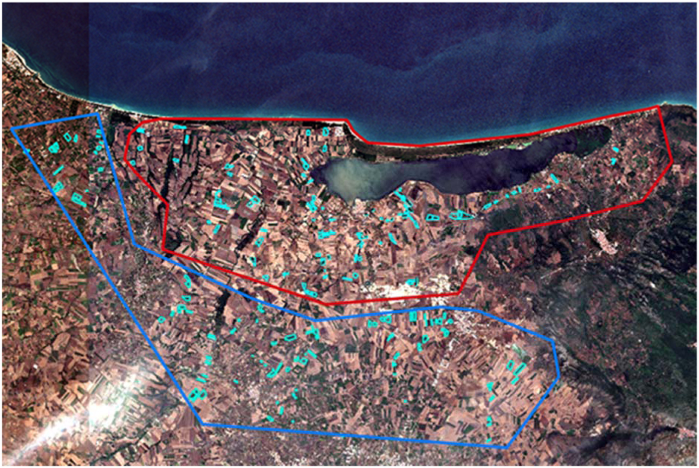
Fig. 6. Lesina area affected by a hailstorm in June 2016 (in red), and the neighbouring control area (in blue); in the background Google imagery is shown, with affected areas under tomato (as indicated by local producers’ association) highlighted in light blue.
The statistics of the affected and control areas were compared, hypothesizing the presence of damage in those tomato fields having TG values below those of the control area. An analysis of TG statistics was also performed between the S2 dated 23 May and a RapidEye image dated 17 June 2016, both pre-event, to better evaluate the TG trend. The results were tested using Student's t test.
Analyses were conducted using ENVI software (Exelis Visual Information Solutions, Boulder, Colorado, USA), and MATLAB and Statistics Toolbox (The MathWorks, Inc., Natick, Massachusetts, USA).
Results
The early quantitative estimate of tomato surface was 2500 ha in CC, 1300 ha in CPS and 20 300 in PMB. The comparison of these values with tomato surfaces estimated per area by classification (illustrated in Table 1) for these specific three areas reveals that larger differences in surface between early estimates and final tomato classifications are found in CPS (+29.8%), compared with CC (+6.9%), with only minor differences found for PMB area (+2.3%).
The overall accuracies of the ML classifications for each area, with details for tomato class producer and user accuracies, number of crop types and number of tomato validation pixels, are presented in Table 3. The tomato class results showed producer accuracy ranging from 0.684 to 0.990, with values >0.80 in seven cases out of nine, and user accuracy ranging from 0.564 to 0.999, with values >0.80% in five cases out of nine. With regard to inputs used, vegetation indices alone were not able to provide satisfactory results; classification results were obtained using stacked bands in four areas (CPS, Lazio sud, Puglia sud, TN), stacked bands plus NDVI in one area (PMB) and bands plus both vegetation indices in two areas (CC, Toscana sud–Lazio nord).
Table 3. Summary data for the classification of the seven study areas

OA, overall accuracy; κ, κ coefficient; and total number of crop types. Data for tomato, extracted from areas classifications: PA, producer accuracy; UA, user accuracy; and validation pixels. Study areas: TN, Toscana nord; TL, Toscana sud–Lazio nord; LS, Lazio sud; CC, Campania casertano; CPS, Campania Piana del Sele; PMB, Puglia nord, Molise, Basilicata; PS, Puglia sud.
The Pearson coefficient of correlation between tomato user/producer accuracies and number of classes was calculated: moderate negative correlations for both producer (r = –0.45) and user (r = –0.50) accuracies were found. The correlation between number of pixels employed in validation and tomato users/producer accuracy was also calculated: results indicate moderate negative correlations with user (r = –0.62) and producer (r = –0.57) accuracies.
The second tomato validation was carried out in CC only, after refinement by photointerpretation of aerial data. Table 4 compares tomato producer and user accuracies, over the same fields, obtained before (at first classification of satellite data) and after refinement (after using aerial information).
Table 4. Comparison of results obtained pre- and post-refinement with aerial data, for field surveyed in rapid field assessment

CC, Campania casertano.
For evaluation of damage caused by a hailstorm in the Lesina area, the statistics for TG calculated using pre- and post-event S2 images are illustrated in the upper part of Table 5. Results indicate that in the control area, the NDVI of the post-event image is approximately 1.5 times higher than that of the pre-event image. The Student's t test revealed significant (P < 0.01) results in Lesina and the control areas.
Table 5. Tomato growth statistics in the hailstorm and control area computed using pre- and post-event S2 images (upper part) and pre-event S2 and RapidEye images tomato growth rate: TG = (NDVI22/06−NDVI23/05)/NDVI23/05

With respect to damage extent and evaluation, it was considered that fields were damaged when TG in the affected areas was lower than ‘mean−(2 × s.d.)’ of TG in the control area. According to this, 179 ha was identified as damaged, equal to 0.10 of the hectares of tomato in the control area, a value similar to that (approximately 200 ha) informally reported by a local producer organization.
The pre-event TG statistic based on S2 and RapidEye images, computed to evaluate the similarity of the NDVI response between two different imagery types, is illustrated in the lower part of Table 5: it shows that values from the two sensors are very similar, in accordance with the hypothesis that the observed decrease in TG can be attributed to the hailstorm event. The Student's t test result for TG in Lesina and the control area was significant (P < 0.01).
The original classifications are shown at the end of the manuscript in Tables 6 to 14. Figure 7 illustrates a tomato final map for PMB area.
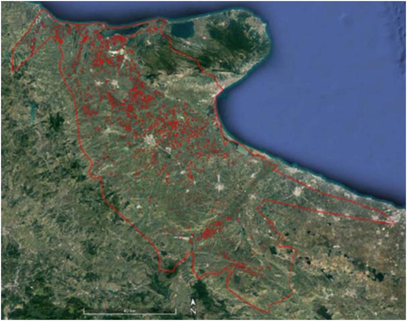
Fig. 7. Tomato map for Puglia nord, Molise, Basilicata (PMB) area, visualized over a real colour Landsat imagery (in Google Earth Pro); in red the tomato fields and the area boundary.
Table 6. Toscana nord ML classification

Table 7. Toscana sud–Lazio nord ML classification

Table 8. Lazio sud ML classification

Table 9. Campania casertano ML classification

Table 10. Campania Piana del Sele ML classification

Table 11. Puglia, Molise, Basilicata 1 ML classification

Table 12. Puglia, Molise, Basilicata 2 ML classification

Table 13. Puglia, Molise, Basilicata 3 ML classification

Table 14. Puglia sud ML classification

Discussion
The early quantitative estimate of tomato-cultivated surfaces, realized in mid-June (about 1–8 weeks from transplanting), was based on the frequency of occurrence of tomato in the field survey; it did not exploit remote-sensing data because in most cases crop development is too limited for remote detection at that stage. The comparison of these early quantitative estimates with the surfaces derived from the ML classifications (obtained a few weeks later) indicates differences, which are variable according to the study site. The lowest difference, hence best result, was found in PMB: this result was attributed in part to the early transplanting dates caused by warmer climate, and also to the larger size of agricultural fields and better road network. Both factors facilitate the collection of evenly distributed and representative tomato ground truth and thus may lead to more accurate early estimates. Conversely, the highest differences between early estimated and classified tomato surface are found in CPS, an area characterized by landscape fragmentation, topographic heterogeneity, limited mean field size and less diffuse road network. These early results must be viewed with caution: the early quantitative estimate method did not allow validation, surveys were carried out when tomato recognition is most difficult and when some transplanting remained to be done, and the sampled surface was limited. In addition, the limits imposed to sampling design – due to field accessibility problems – and ground truth data collection may have played a role in the obtained results. Nevertheless, this procedure can be still valuable for stakeholders interested in very early indications on the total amount of cultivated tomato for the season.
The ML classifications for all crops were obtained in mid-July, a time when most of the crops are at an early stage of development, especially in central-northern regions. The ML algorithm was selected to keep the procedure simple and replicable by users. Despite the early date, two-thirds of the classifications were >0.80 overall accuracy (OA) threshold, with values included in the 0.60–0.87 range. Overall, the obtained OAs are lower than those found in agricultural studies employing very-high-resolution satellite data, which often record OAs >0.80 (Conrad et al., Reference Conrad2010, Reference Conrad, Neale, Maltese and Richter2011; Hoberg and Müller, Reference Hoberg and Müller2011; Kim et al., Reference Kim, Yeom, Kim, Neale, Maltese and Richter2011; Löw et al., Reference Löw and Habib2012). However, those studies are usually based on multitemporal very-high-resolution images, are realized at full stage of crop development and include a very limited number of classes. The results obtained by the few available classification studies based on real or simulated S2 data (Hale Topaloglu et al., Reference Hale Topaloglu, Sertel and Musaoglu2016; Immitzer et al., Reference Immitzer, Vuolo and Atzberger2016; Sibanda et al., Reference Sibanda, Mutanga and Rouget2016; Vaglio Laurin et al., Reference Vaglio Laurin2016) are comparable in OA to those obtained in the present study. The current paper included the overall classification of the study areas in the results, including all crops, even though the primary focus was tomato mapping. This choice was motivated by the scarcity of this type of information in Italy and the information content on heterogeneity, class number and crop types per area (crops have different spectral similarity with tomato). In addition, overall the results prove that, even at an early stage of crop development and in the presence of a high number of crop types, S2 is capable of providing reasonable accuracy in crop mapping.
The accuracies obtained with S2 possibly indicate that its spectral characteristics are very important: S2 10–20 m spatial resolution may not be optimal with respect to the smaller tomato fields still found in the study areas (even though the average field area was found to be in the 2–4 ha range). In fact, the very irregular shape of some fields and mixed crop practices may lead to the inclusion in pixels of information coming from other crops, even though a buffer to the external field perimeter was applied. Possibly, the S2 10–20 m spatial resolution limit was compensated for by the increased spectral information content. Lower spectral information can lead to higher misclassification of spectrally similar crops; enhanced spectral resolution is thus especially useful when crop discrimination is performed at the beginning of vegetation development.
User/producer accuracy for tomato class was over the 0.80 threshold in most cases. Still, variability in accuracy results was observed: correlation analysis indicates that accuracy is partly affected by the increase in number of classes. It is reasonable to argue that the heterogeneity of agricultural areas has an impact on the ability to correctly classify tomato fields, and the task becomes more challenging when more species and spectral variability are present. The presence of different soil types and moisture levels can have an important role in shaping the observed area heterogeneity and variability in the results. The amount of exposed soil can be relevant at early stages of vegetation development, producing confounding effects in classification, as previously observed in other studies (Montandon and Small, Reference Montandon and Small2008; Belgiu and Csillik, Reference Belgiu and Csillik2018).
The second validation results, performed after improving tomato maps by means of photointerpretation of aerial data and collected over part of the CC area, showed an increase in producer accuracy (+7%) and a minor decrease in user accuracy (−2.5%). This reduction in omission errors, at similar rate of commission errors, suggests the usefulness of aerial data in tomato classification efforts as additional surrogate ground truth. It is worth noting that the second validation showed accuracy values slightly lower than those obtained in S2 classifications. A possible interpretation is that the limited number of samples used for training and validation of classifications, due to the chance of sampling only a minor percentage of the study areas, led to an overestimation of tomato accuracy, especially in those areas validated with fewer pixels. This interpretation is also supported by the moderate negative correlation between tomato accuracies and number of validation pixels observed. In addition, the second validation was conducted on a field basis, while the classifications were produced with a pixel-based approach; this difference may have introduced additional variability. Even if the second validation campaign was conducted in a single area only, the use of aerial information is recommended in selected sub-areas having complex topography or high crop heterogeneity.
The results of tomato damage evaluation indicate that S2 is valuable for monitoring crop growth; the similarity in response between S2 and RapidEye in pre-damage conditions also confirms the optimal spectral calibration of S2 data. The damage detection capability is clearly linked to the date of damage occurrence; in this specific case, the hailstorm happened in the second half of June, in an area of early transplanting dates and therefore at a medium stage of tomato development. If damage occurs soon after transplanting, detection ability may decrease consistently. Even if there is no availability of proper validation data to confirm the accuracy of estimated damaged surface, the clear change in NDVI supports the use of S2 for damage detection and growth changes in crops.
Conclusions
The current study documents the procedure to obtain early information on tomato-planted areas and maps, a task which is considered not trivial due to the limited development of plants at the time of information production and due to environmental heterogeneity of the agricultural areas. Ground data, S2 satellite data and a very-high-resolution airborne multispectral data were all used to deliver the timely tomato information requested by the users.
In general, the results indicate that early quantitative estimate of tomato-cultivated surfaces are possible in these study areas, but their accuracy depended on the heterogeneity of the environment and the agricultural practices, with better results obtained in homogeneous and southern areas, where early transplants take place. The S2 data classified tomato with satisfactory accuracy, even in the presence of multiple crop types, thanks to its enhanced spectral features. However, the number of crop types impacted the accuracy of the results, and the use of aerial data as surrogate ground truth is recommended in sub-areas having high heterogeneity or complex topography. Sentinel 2 was also demonstrated to be a valuable tool for crop growth monitoring and crop damage assessment.
At full operating parameters, S2 provides very frequent acquisitions, increasing the chance of cloud-free data at no cost – cloud cover being one of the major limitations for the production of information for users’ needs. The possibility to integrate S2 with other satellite data, such as free all-weather Sentinel 1 SAR, is another feature in favour of the use of S2 for species-level crop monitoring. On-demand satellite data are acquired in the absence of clouds: however, not only are these data expensive, but acquisition dates cannot be controlled completely, as a sufficient temporal window (usually >20 days) is requested by data provider. It may be that acquisitions are performed at the very beginning of the temporal window, thus in an early stage of crop development in which crop distinction is unfeasible. These considerations, together with the presented results, indicate that S2 can be successfully employed to provide users with early information on specific crops.
Financial support
G.V.L and D.P. acknowledge the European Union for supporting the BACI project funded by the EU's 692 Horizon 2020 Research and Innovation Programme under grant agreement #640176.
Conflict of interest
None.
Ethical standards
Not applicable.


