

1 Introduction
Best estimates of an economic parameter are subject to both publication selection bias as well as the bias induced as part of the judgmental process in choosing the “best” estimate from each study, or what this article terms “best estimate selection bias.” The potential influence of these biases is of general pertinence to economic policies as the choice of economic parameters to use in policy analyses is an intrinsic aspect of such efforts. There may be fundamental policy ramifications if there is an impact of such biases on estimates of parameters that are influential components of policy assessment, such as the value of a statistical life (VSL), which is the focus of this article. The VSL, which is the tradeoff rate between money and fatality risks, is the most important single economic parameter influencing the evaluation of government regulations.Footnote 2 Labor market estimates of VSL serve as the principal basis for the valuation of mortality risks from a broad range of regulations, such as environmental and transportation regulations.Footnote 3
In their selection of the VSL estimate for policy purposes, U.S. government agencies have often drawn on the implications of meta-analyses and meta-regression studies. Usually, government agencies have relied on estimates from studies that provide broad overviews of the literature, such as Viscusi (Reference Viscusi1993), Mrozek and Taylor (Reference Mrozek and Taylor2002), Viscusi and Aldy (Reference Viscusi and Aldy2003) and Kochi, Hubbell and Kramer (Reference Kochi, Hubbell and Kramer2006). Agencies also have undertaken their own review of the estimates in the literature, such as the U.S. Department of Transportation’s (2016) review and synthesis of labor market estimates based on more recent fatality rate data, which led to the department’s current VSL estimate of $9.4 million. The U.S. Environmental Protection Agency (2016) uses a similar VSL of $9.7 million (in 2013 dollars), and the U.S. Department of Health and Human Services (2016) uses a value of $9.6 million (in 2014 dollars). There have been numerous meta-regression analyses of the VSL estimates, as researchers have used this approach to minimize the estimation error across the VSL estimates and to address potential biases from the omission of pertinent variables from the analysis.Footnote 4 However, none of the meta-analysis studies that have been used by government agencies for policy purposes has sought to account for the role of publication selection effects.
This failure to adopt publication-bias-corrected estimates is not unique to estimates of the VSL, as there appear to be no examples of government agencies adopting such corrections. A principal contributor to current practices is that the statistical techniques for adjusting for publication bias are fairly novel, as the systematic approaches using meta-regression techniques are less than two decades old. As a result, there is not a substantial literature in which analysts have shown that correction for such biases is both feasible and consequential. In addition, government agencies may wish to see that the initial bias corrections identified in the literature are corroborated in other studies before abandoning well-established policy analysis practices. As will be discussed below, the first published estimates of the VSL correcting for publication selection effects demonstrated substantial reductions in the VSL that would have drastically reduced benefit assessments and the optimal policy mix. Since subsequent estimates derived from the VSL estimates based on more recent fatality data are more in line with existing practices, awaiting the results of additional research is sometimes desirable.
Much of the impetus for the concern with the potential effects of publication selection biases on published statistics emerged in the context of research on publication selection bias in the medical literature. The two principal types of bias that were identified for randomized control trials of medical interventions were outcome reporting bias and publication bias (Dwan et al., Reference Dwan, Altman, Arnaiz, Bloom, Chan, Cronin, Decullier, Easterbrook, Von Elm, Gamble, Ghersi, Ioannidis, Simes and Williamson2008, Reference Dwan, Gamble, Williamson and Kirkham2013). Many research results are never published because the researchers or the funders of the work often did not have an interest in publishing results of unproductive lines of inquiry. In addition, there is a potential bias that arises because researchers are less likely to submit articles for publication if the results are not statistically significant. Similarly, some journals may be less likely to publish results with statistically insignificant results. Novel results also may encounter mixed prospects. In some instances, there may be resistance to publishing results not consistent with previous research. The opposite problem may arise as well, as there is sometimes a bias toward publishing results that are viewed as particularly path-breaking, which often happens in the medical literature for novel small effects that are subsequently refuted (Ioannidis, Reference Ioannidis2005).
Recent contributions have found that similar types of biases may affect studies in the economic literature.Footnote 5 There is also evidence of statistically significant publication selection effects for estimates of the VSL, consistent with the concerns expressed in Ashenfelter and Greenstone (Reference Ashenfelter and Greenstone2004) and Ashenfelter (Reference Ashenfelter2006). Utilizing a sample of the best estimates of the VSL, Doucouliagos, Stanley and Giles (Reference Doucouliagos, Stanley and Giles2012) found that accounting for the influence of publication bias reduced the mean estimates of the VSL by 70%–80%. The extent of the bias is, however, much less pronounced for more recent estimates based on the Bureau of Labor Statistics Census of Fatal Occupational Injuries (CFOI) data (Viscusi, Reference Viscusi2015).
This article uses established techniques for evaluating publication selection effects to examine the magnitude and direction of bias based on meta-regression analyses of a dataset consisting of the “best set” of VSL estimates in which researchers selected the single best estimate from particular articles, as well as an “all-set” dataset that includes all VSL estimates reported in those studies.Footnote 6 Each of these sets of results is subject to the same sources of biases, but to a different degree. The all-set results initially reflect the decision by the author regarding which estimates to submit for publication, or outcome reporting bias. The estimates submitted by the author may include the author’s preferred model as well as a variety of different specifications to show the sensitivity of the results to other specifications of the econometric model. The estimates submitted by the author to the journal in turn are subject to reviewer reports and approval by the journal editors, who may propose trimming some estimates from the paper or may suggest that the author present alternative specifications, such as analysis of different sample groups (e.g., male workers or blue-collar workers) or alternative constructions of the fatality rate variable (e.g., use of lagged values). The set of decisions by the author and by the journal editors regarding what should be published leads to the VSL estimates in the all-set sample. Of this all-set group, the best-set estimate is the single estimate that the author views as most credible. Thus, the best-set estimate sets aside the robustness tests presented by the author or suggested by the journal editors and places greater weight on a focal estimate. However, in choosing this focal estimate, there may be an additional bias that is engendered. The author might, for example, select a VSL estimate that is consistent with past studies, possibly including estimates in articles by the reviewers or journal editors, to enhance the likelihood of the paper’s acceptance for publication and to bolster the general acceptance of the results.
The specific focus here extends beyond the standard characterization of publication selection bias to estimate the extent to which the best estimate selection process induces an additional source of bias, which this article terms “best estimate selection bias.” In particular, the subjective process of selecting the “best estimate” of the VSL from particular studies may introduce additional biases beyond the standard selection biases that are generated by the process by which research results are reported and published. There may, of course, be sound statistical reasons for authors to prefer some econometric estimates of economic parameters to others. Use of superior fatality rate data and inclusion of a more comprehensive set of key explanatory variables are two prominent examples of factors that one might wish to take into account. However, it is also feasible to incorporate such influences within the context of a comprehensive meta-regression analysis controlling for pertinent characteristics of the different models or to undertake a publication-bias-corrected analysis of an all-set sample of sound studies.
That there might be publication selection bias in the VSL estimates was first established by Doucouliagos et al. (Reference Doucouliagos, Stanley and Giles2012), who estimated a bias-corrected VSL estimate of $1.1 million using a best-set sample of 39 studies. The results reported in Viscusi (Reference Viscusi2015) updated their database and similarly found bias-corrected VSL estimates on the order of $1–$2 million (in 2013 dollars) for best-set samples ranging from 39 to 60 studies. However, the best-set estimates conditional on the fatality rate data derived from the CFOI data were higher, as were the all-set estimates that were restricted to the VSL estimates based on the CFOI data. The present article expands on the best-set analysis, including eight additional studies not included in Viscusi (Reference Viscusi2015). The more important difference is that this article presents the first analysis to include all 1025 VSL estimates from these 68 studies, making it possible to contrast the results from the best-set estimates and the all-set estimates. The principal result is that the surprisingly low bias-corrected VSL estimates in Doucouliagos et al. (Reference Doucouliagos, Stanley and Giles2012) and the update of that analysis in Viscusi (Reference Viscusi2015) stemmed from the reliance on the best-set estimates rather than all VSL estimates that were reported. Even without making predictions conditional on whether the studies used the CFOI data, based on predictions from the preferred econometric specifications, the overall mean bias-corrected estimate for the full sample is $8.1 million and $8.0 for the USA sample, which are very similar to the values used by U.S. government agencies. The estimates conditional on CFOI data yield even greater bias-corrected values. The apparent evidence of enormous publication selection biases in labor market estimates of the VSL is largely attributable to the impact of best estimate selection bias rather than an underlying publication selection bias. Government agencies’ reliance on the VSL estimates in the literature is well founded.
Section 2 of this article introduces both a best-set dataset, including the best estimates of VSL from a series of studies, and an all-set dataset, including all VSL estimates from these studies. The distribution of the VSL estimates in each instance is suggestive of possible publication selection effects, with greater apparent selection effects for the best-set data. Section 3 presents bias-corrected estimates for the all-set data, finding evidence of significant and substantial publication bias. Section 4 presents the counterpart analysis for the best-set estimates and a comparison with the all-set results. The starkly greater selection corrections for the best-set estimates lead to bias-corrected estimates well below the values currently used in policy assessment. As indicated in the concluding Section 5, there is evidence of statistically significant selection effects in each instance, but the far greater extent of the biases for the best-set estimates indicates the powerful impact of best estimate selection bias.
Nevertheless, the process of selecting the best estimates of the VSL has yielded mean and median estimates that do not differ greatly from those that are derived from the all-set sample. Despite the evidence that standard statistical procedures for adjusting for publication selection biases document the presence of substantial selection effects, the mean and median estimates of both the best-set estimates and the all-set estimates are in a reasonable range, but the distributions differ. The overall performance of the best estimate selection means and medians is reminiscent of the classroom situation in which students sometimes get the right answer for the wrong reasons. Similarly, the estimated biases induced by the best estimate selection process are considerable, but the judgments regarding the appropriate magnitudes of the VSL drawn from these studies largely affects both tails of the distribution.
The potential impacts of best estimate selection effects have broad implications for economic analyses as the selection of different economic parameters for analytic purposes often relies on subjective judgment of the best estimate of the parameter. The findings presented here demonstrate that best estimate selection bias may induce serious additional selection effects in addition to those that result from publication selection effects.
2 All-set data, best-set data, and VSL distributions
2.1 Summary statistics
The focus of this meta-analysis is on labor market estimates of the VSL. The estimates using labor market data constitute the largest group of revealed preference estimates of the VSL in the economics literature as well as the largest set of meta-analysis studies. The set of valuations considered in this article consists of published estimates of the VSL as well as estimates that are forthcoming in economics journals. The universe of studies included in this analysis encompasses all analyses included in the meta-analyses by Viscusi and Aldy (Reference Viscusi and Aldy2003), Bellavance, Dionne and Lebeau (Reference Bellavance, Dionne and Lebeau2009) and Viscusi (Reference Viscusi2015), as well as subsequent articles written after the time period included in these meta-analyses, including all U.S. studies identified using an EconLit search for the VSL. Appendix A provides a list of the studies used in the analysis. This article uses two datasets: a meta-analysis of best estimates of the VSL from 68 studies and a meta-analysis consisting of the full set of 1025 VSL estimates reported in these studies.
The canonical hedonic labor market model used to estimate the VSL is either a wage equation or a log wage equation in which the explanatory variables include the fatality risk for the worker’s job and other variables. The wage equation takes the general form:
 $$\begin{eqnarray}\text{wage}_{i}=\unicode[STIX]{x1D6FD}_{0}+\unicode[STIX]{x1D6FD}_{1}\text{ fatality rate}_{i}+X_{i}^{\prime }\unicode[STIX]{x1D6FD}_{2}+\unicode[STIX]{x1D700}_{i},\end{eqnarray}$$
where $\mathit{wage}_{i}$
is the worker
$\mathit{wage}_{i}$
is the worker $i$
’s hourly wage rate,
$i$
’s hourly wage rate, $\unicode[STIX]{x1D6FD}_{0}$
is the constant term,
$\unicode[STIX]{x1D6FD}_{0}$
is the constant term, $\unicode[STIX]{x1D6FD}_{1}$
is the key coefficient of interest,
$\unicode[STIX]{x1D6FD}_{1}$
is the key coefficient of interest, $\unicode[STIX]{x1D6FD}_{2}$
is a vector of coefficients, fatality rate is the annual fatality rate for the worker’s job, and
$\unicode[STIX]{x1D6FD}_{2}$
is a vector of coefficients, fatality rate is the annual fatality rate for the worker’s job, and $X_{i}$
is a vector of variables pertaining to worker
$X_{i}$
is a vector of variables pertaining to worker $i$
’s personal characteristics, the worker’s job, and regional characteristics. The coefficient
$i$
’s personal characteristics, the worker’s job, and regional characteristics. The coefficient $\unicode[STIX]{x1D6FD}_{1}$
corresponds to the wage-risk tradeoff in terms of the wage premium per unit risk. After appropriate adjustment of units,
$\unicode[STIX]{x1D6FD}_{1}$
corresponds to the wage-risk tradeoff in terms of the wage premium per unit risk. After appropriate adjustment of units, $\unicode[STIX]{x1D6FD}_{1}$
corresponds directly to the VSL. To convert the hourly wage premium for risk into units comparable to the annual fatality rate variable based on a full-time work year, the coefficient
$\unicode[STIX]{x1D6FD}_{1}$
corresponds directly to the VSL. To convert the hourly wage premium for risk into units comparable to the annual fatality rate variable based on a full-time work year, the coefficient $\unicode[STIX]{x1D6FD}_{1}$
is multiplied by 2000, which is a measure of the annual number of hours worked if the worker is full time. There also may be scale adjustments to account for the units of the fatality rate variable, e.g., if the risk is per 100,000 workers. The estimate of
$\unicode[STIX]{x1D6FD}_{1}$
is multiplied by 2000, which is a measure of the annual number of hours worked if the worker is full time. There also may be scale adjustments to account for the units of the fatality rate variable, e.g., if the risk is per 100,000 workers. The estimate of $\unicode[STIX]{x1D6FD}_{1}$
and its standard error thus correspond to the VSL and the standard error of the VSL except for a multiplicative scale term.
$\unicode[STIX]{x1D6FD}_{1}$
and its standard error thus correspond to the VSL and the standard error of the VSL except for a multiplicative scale term.
The semi-logarithmic form of the equation is of the form:
 $$\begin{eqnarray}\text{ln wage}_{i}=\unicode[STIX]{x1D6FD}_{0}+\unicode[STIX]{x1D6FD}_{1}\text{ fatality rate}_{i}+X_{i}^{\prime }\unicode[STIX]{x1D6FD}_{2}+\unicode[STIX]{x1D700}_{i}.\end{eqnarray}$$
Although there is no theoretical basis for adopting a particular functional form in hedonic wage studies, the semi-logarithmic form performs better based on Box–Cox specification tests and is more widely used in the literature. Calculating the VSL based on equation (2) requires more than the aforementioned scale adjustments. The VSL derived from equation (2) is not estimated based on a single coefficient, but rather is given by:
 $$\begin{eqnarray}\text{VSL}=\unicode[STIX]{x2202}\text{wage}/\unicode[STIX]{x2202}\text{fatality rate }=\hat{\unicode[STIX]{x1D6FD}}_{\text{1}}\times \overline{\text{wage}}.\end{eqnarray}$$
While the VSL can be evaluated at any point in the wage distribution based on the estimated wage-risk tradeoff rate $\hat{\unicode[STIX]{x1D6FD}}_{1}$
, the usual procedure is to evaluate the VSL for the mean wage rate, which is an estimated value rather than a known value. In addition to the error in the estimate of
$\hat{\unicode[STIX]{x1D6FD}}_{1}$
, the usual procedure is to evaluate the VSL for the mean wage rate, which is an estimated value rather than a known value. In addition to the error in the estimate of $\unicode[STIX]{x1D6FD}_{1}$
, wage is a random variable, which in turn will affect the calculated error for VSL when evaluating the VSL at the mean wage rate. This complication does not arise if the
$\unicode[STIX]{x1D6FD}_{1}$
, wage is a random variable, which in turn will affect the calculated error for VSL when evaluating the VSL at the mean wage rate. This complication does not arise if the $\overline{\mathit{wage}}$
value is known or if the VSL is evaluated at a known specific value in the wage distribution.
$\overline{\mathit{wage}}$
value is known or if the VSL is evaluated at a known specific value in the wage distribution.
Table 1 Summary statistics for all-set and best-set samples.

The subsequent meta-analysis of VSL encompasses five groups of variables in Table 1. The first group consists of characteristics of the estimates. The average VSL is $12.0 million for the all-set sample and $12.2 million for the best-set sample, where all dollar figures in this article are in 2015 dollars based on the CPI-U. Focusing simply on the overall average VSL yields similar estimates for both the all-set and best-set samples. Table 1 also reports the standard error of the VSL estimate, which will play a pivotal role in the subsequent analysis of publication selection bias. Appendix B summarizes the procedure used to construct the standard errors of the VSL that were missing and could not be constructed for some studies. No other variables had any observations for which the values needed to be imputed. The next two variables are the average annual income and log of the annual income (ln income) for the different samples used in the studies. Annual income converts the worker’s hourly wage to an annual income figure assuming 2000 hours worked per year, which is an approach consistent with the full-time work assumption generally used in constructing governmental fatality rate figures. These variables can be included in the analysis below to account for the potential income elasticity of the VSL. All subsequent variables listed in Table 1 are 0–1 indicator variables.
A series of six variables captures differences relating to the equation specification and the types of standard errors. The variable workers’ compensation is a 0–1 indicator variable for whether the wage equation included a workers’ compensation benefit measure, which 27% of the articles did. Just over one third of all the reported estimates and just under half of all articles included a nonfatal injury variable in the hedonic wage equation. Ten percent of the estimates and 4% of the articles utilized a wage specification, as the semi-logarithmic form is more prevalent. The variable CFOI indicates whether the equation used a fatality rate measure based on the Census of Fatal Occupational Injuries (CFOI) data. These data are the highest quality worker fatality rate data as they are based on a comprehensive census of all U.S. occupational fatalities, where each fatality is verified using multiple sources (Viscusi, Reference Viscusi2013). Other fatality rate data are deficient in one or more respects, such as being based on voluntary industry reporting from a partial sample of firms. Given the presence of the wage variable in the VSL calculation for semi-logarithmic equations, as indicated in equation (3), the variation in the wage variable should be taken into account in the calculation of the standard error of VSL when using the semi-log specification and calculating the VSL for the mean worker. For ease of exposition, I refer to studies that did so as having correct standard errors.Footnote 7 The final equation specification variable, IV estimate, is whether the VSL was estimated using an instrumental variables estimator for the fatality rate.
The final nine variables in Table 1 pertain to the particular sample used in the estimation. Was the sample a USA sample or was it drawn from some other country? Although many studies have used the full sample of workers, others have restricted the analysis to particular groups of workers. The sample groups that are considered include a union sample for workers who were union members or covered by a collective bargaining agreement and a nonunion sample consisting solely of workers who do not belong to a union or are not covered by a collective bargaining agreement. The blue-collar sample and white-collar sample variables characterize different occupation mixes that have been the focus of studies that narrowed the sample to particular occupational groups. The racial differences in the samples are for whether the sample was restricted to workers who are white or who are nonwhite. The final two variables pertain to whether the estimates focused only on workers who are male or who are female.
2.2 VSL distributions and funnel plots
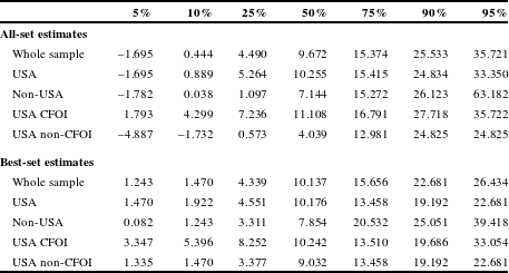
The best-set and all-set distributions are likely to differ since one would not expect authors to select the outlier values as their “best” estimate of the VSL in their study. Table 2 reports the distribution of the VSL estimates for the all-set sample in the upper panel and the best-set sample in the lower panel. The first row of each panel presents the distribution for the whole sample, and the subsequent rows present the distribution for different subsamples of interest: USA samples, non-USA samples, USA studies that used the CFOI data, and USA studies that did not use the CFOI data.
Table 2 Distributions of VSL estimates by quantile.
a
Note: For the all-set sample, $N=1025$
. For the best-set sample,
$N=1025$
. For the best-set sample, $N=68$
.
$N=68$
.
The distribution of the VSL values for the whole sample in Table 2 indicates a tighter distribution of values for the best-set results than the all-set results. The median VSL estimate for the all-set whole sample is $9.7 million, which is similar to the best-set median of $10.1 million, but the distributions differ. The 95th percentile for the whole sample is $35.7 million for the all-set estimates and $26.4 million for the best-set estimates so that there is some muting of the values at the upper end for the best-set sample. The upper end of the distribution exhibits a greater difference from the median than the lower end of the distribution. The VSL spread in the whole sample between the median and the 95th percentile is more than double the difference between the 5th percentile and the median for the all-set estimates, and is somewhat less than double that difference for the best-set estimates, which are more compressed. There is a particularly pronounced difference at the left tail, as the 5th percentile best-set estimate for the whole sample is $1.2 million, which exceeds the negative 5th percentile value of –$1.7 million for the all-set results and also exceeds the 10th percentile all-set value of $0.4 million.
The patterns for the different subsamples are similar to the whole sample in terms of the median values, except for the USA non-CFOI studies, as the all-set median for the USA CFOI studies is $11.1 million as compared to $4.0 million for the USA non-CFOI all-set sample. The all-set estimates are lower than the best-set estimates at the 5th percentile and greater at the 95th percentile. The 5th percentile VSL estimates for the all-set sample are negative, with the exception of the CFOI sample results. The 5th percentile values for the best-set estimates are always positive.
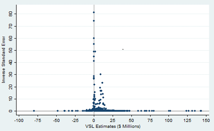
The potential impact of publication selection bias is evident in an examination of the distribution of the VSL estimates based on an approach developed by Egger, Smith, Schneider and Minder (Reference Egger, Smith, Schneider and Minder1997) and Stanley (Reference Stanley2008). It is useful to characterize the estimates graphically, with the inverse of the standard error of the VSL estimate on the vertical axis and the VSL estimate on the horizontal axis. The estimates with the smallest standard error are the most precise estimates, and these will be highest on the funnel plot vertical axis. The most precisely estimated VSL levels also are instrumental in the subsequent estimation of the publication-bias-corrected VSL. In the absence of publication selection bias, one would expect the VSL estimates to be uncorrelated with the standard error for studies of populations with similar distributions of VSL. Situations in which workers’ VSL levels are high because of factors such as differences in preferences will lead to larger VSL estimates and larger standard errors. There may, of course, be differences in the VSL and the associated standard errors stemming from influences such as income levels, but these will be taken into account below in the meta-regression counterpart of this funnel plot analysis. If there is no publication selection bias, the estimates of VSL should be symmetrically distributed in such graphs around the mean estimated value, with a shape that has the appearance of an inverted funnel.

Figure 1 Funnel plot of VSL estimates for the all-set sample. Note: $N=1025$
.
$N=1025$
.
Figure 1 provides the funnel plot for the all-set sample of VSL estimates. Both positive and negative VSL values are evident, though there is some apparent reluctance of researchers to report theoretically implausible negative estimates. Positive VSL estimates appear to be an influential model selection criterion. In particular, there is clustering of the small positive values coupled with an upper right tail of the distribution that extends farther than does the left tail. This overall pattern is consistent with the presence of some publication selection bias, which will be examined more formally below.
The funnel plot for the best-set sample in Figure 2 is much more skewed than the all-set distribution, as it has a completely asymmetric appearance and is strongly right-skewed. This distribution is truncated at the vertical axis. There are no negative estimates reported as the best estimates in any of the articles. This tendency reflects what is known as directional publication bias in which results inconsistent with established economic theories regarding the direction of the effect are less likely to be published. The directional publication bias in turn tends to reflect the average size of the VSL estimate. Many of the reported values are clustered at or to the right of the vertical axis. The graphical depictions in Figures 1 and 2 suggest that there is likely to be greater publication selection bias in the best-set estimates than if all reported estimates are considered.

Figure 2 Funnel plot of VSL estimates for the best-set sample. Note: $N=68$
.
$N=68$
.
Although these funnel plots do not provide formal tests of publication selection effects, they are strongly suggestive of the presence of such influences. Moreover, there appears to be an asymmetry to the effects, with there being a greater reluctance to report estimates at the left tail of the distribution than very high estimates. One consequently might expect econometric corrections for these biases to reduce rather than increase the estimated VSL.
3 Meta-regression estimates of selection-corrected VSL for the all-set sample
To control for potential heteroskedasticity, the first set of meta-regression estimates consists of weighted least squares (WLS) estimates of VSL estimates for both the full set and best set of VSL values using as weights the inverse of the variance of the VSL estimates.Footnote
8
The initial regression is of the VSL on its estimated standard error for each observation $j$
. In particular, the equation takes the form:
$j$
. In particular, the equation takes the form:
 $$\begin{eqnarray}\text{VSL}_{j}=\unicode[STIX]{x1D6FC}_{0}+\unicode[STIX]{x1D6FC}_{1}\text{ standard error}_{j}+\unicode[STIX]{x1D700}_{j}.\end{eqnarray}$$
The statistical significance of the coefficient $\unicode[STIX]{x1D6FC}_{1}$
for the standard error variable in this equation is the test of the presence of publication selection bias. The constant term in this model
$\unicode[STIX]{x1D6FC}_{1}$
for the standard error variable in this equation is the test of the presence of publication selection bias. The constant term in this model $\unicode[STIX]{x1D6FC}_{0}$
is the publication selection bias-corrected estimate of VSL.
$\unicode[STIX]{x1D6FC}_{0}$
is the publication selection bias-corrected estimate of VSL.
A more comprehensive version of this equation includes additional covariates given by the vector $X_{j}$
and is given by:
$X_{j}$
and is given by:
 $$\begin{eqnarray}\text{VSL}_{j}=\unicode[STIX]{x1D6FC}_{0}+\unicode[STIX]{x1D6FC}_{1}\text{ standard error}_{j}+X_{\!j}^{\prime }\unicode[STIX]{x1D6FC}_{2}+\unicode[STIX]{x1D700}_{j}.\end{eqnarray}$$
In this instance, the inclusion of the standard error term provides a measure of the impact of selection bias, but the constant term does not correspond to the publication-bias-corrected estimate of the VSL.Footnote
9
Instead, one computes the mean bias-adjusted estimate of the VSL based on this equation after setting the value of the standard error term equal to zero and setting the values of the $X_{i}$
variables at their mean levels.
$X_{i}$
variables at their mean levels.
The covariates serve two principal roles. Some variables reflect underlying heterogeneity in the VSL, as in the case of income variations in the VSL. The sample composition variables likewise may capture differences in the supply and demand for workers in potentially hazardous jobs. Other variables, such as the nonfatal injury variable, capture differences in equation specification and included multivariate controls.
Table 3 WLS VSL regressions for the all-set sample.

a
Note: $N=1025$
. Standard errors clustered on labor data source in parentheses. 95% confidence intervals provided in parentheses below VSL estimate standard errors.
$N=1025$
. Standard errors clustered on labor data source in parentheses. 95% confidence intervals provided in parentheses below VSL estimate standard errors. $^{\ast \ast \ast }p<0.01$
,
$^{\ast \ast \ast }p<0.01$
, $^{\ast \ast }p<0.05$
,
$^{\ast \ast }p<0.05$
, $^{\ast }p<0.1$
.
$^{\ast }p<0.1$
.
The regression results in Table 3 report the WLS estimates of the VSL equations (4) and (5). Appendix C presents comparable results using both fixed-effects and random-effects panel models. The reported standard errors in Table 3 are robust standard errors that are clustered by labor market data source. For example, there are multiple articles that use the Current Population Survey or the Panel Study of Income Dynamics as the employment dataset, though the studies often differ by sample composition and year. In recognition that the multiple observations from a common data source may not be independent (Moulton, Reference Moulton1986; Cameron & Miller, Reference Cameron and Miller2015), the standard errors reported in Table 3 are clustered by employment dataset. Appendix C Table C1 reports three additional standard errors as well: standard errors clustered by article, standard errors clustered by author, and more conventional robust, heteroskedasticity-adjusted standard errors. The statistical significance levels and the implied confidence intervals for the bias-corrected estimates of the VSL are similar for all four sets of standard errors.
The first column of estimates in Table 3 provides the base case estimates, while the second column of estimates in Table 3 includes additional covariates. There is evidence of publication selection bias, as the standard error term is positive and statistically significant. However, the magnitude of the standard error term drops by four fifths once other variables are added to the equation. Much of the difference across studies in the standard errors could stem from heterogeneity of the samples and differences in the types of standard errors that are computed rather than selection biases. For example, a sample that exhibits a high VSL also may have a larger standard error associated with that sample’s VSL irrespective of the role of any publication selection effects.
Several of the additional covariates in Table 3 are statistically significant. The VSL estimates are $8.70 million higher for those studies that use the CFOI data. The stark difference in the performance of studies using the CFOI fatality rate data is consistent with the results in Viscusi (Reference Viscusi2015), which may be attributable in part to the lower measurement error in the CFOI fatality rate variable. The other consistently significant effect is that the VSL estimates are lower for nonwhite samples. The –$10.99 million effect implied by the nonwhite sample coefficient is particularly striking as its magnitude indicates that for nonwhite samples there is little or no compensation for fatality risks. The absence of compensation for nonwhite workers is consistent with previous estimates and models in which there is a separating labor market equilibrium in which nonwhite workers face different labor market offer curves than do white workers and do not receive as substantial compensating differentials for risk (Viscusi, Reference Viscusi, Machina and Viscusi2014).
Utilizing these results, it is possible to calculate different publication-bias-corrected estimates of VSL that provide estimates of the mean VSL under alternative assumptions about the desired equation specification, variable set, and sample. For the base case in Table 3, the constant term in the regression corresponds to the overall mean VSL estimate, which is $0.137 million after setting the value of standard error term equal to zero. This value is 99% lower than the overall mean sample raw VSL and is even below the 10th percentile of the raw VSL distribution in Table 2.
Adjusting for the influence of covariates as well in column 2 of Table 3 makes it possible to account for both publication selection bias as well as the desired specifications of the VSL equation. The WLS estimates clustered standard errors that are reported took into account the presence of multiple observations from particular employment datasets. But there also may be systematic effects in the levels of the estimates that one might wish to take into account in using the estimates to provide different perspectives on the appropriate VSL. The “predicted mean VSL” estimate reported in Table 3 is obtained by setting the standard error effect equal to zero and setting all other coefficients in column 2 of Table 2 at their mean values. This approach yields a publication-bias-corrected estimate of $6.3 million, with a confidence interval of ($5.4 million, $7.2 million) based on the standard errors clustered by dataset. The “predicted mean” is 47% lower than the sample mean. The “alternative mean VSL” reported in Table 3 sets the value of the standard error term equal to zero, sets the first seven covariates in Table 3 equal to their means, and sets all the sample characteristic variables equal to zero, yielding an estimated VSL of $6.9 million. This value abstracts from differences attributable to particular samples and leads to a 42% reduction from the raw mean value for the whole sample. Instead of focusing on various mean predicted values, the “preferred mean VSL” turns on the variables that are desirable components of the specification (workers’ compensation, injury risk, and correct standard errors) and sets at their means the values of ln income, USA sample, and CFOI, and sets equal to zero the value of the other variables, yielding a mean VSL value of $8.1 million, which is 32% less than the raw mean VSL for the whole sample. The “preferred mean VSL (USA)” estimates differ in that they also turn on the USA variable and CFOI, yielding an estimated VSL of $11.4 million, with a confidence interval ($10.8 million, $11.9 million). This mean adjusted value is 5% less than the overall raw mean and is greater than the median estimate. Publication-bias influences are consistently evident, but the effects on the VSL are relatively moderate, particularly for the studies using CFOI data.
4 Weighted least squares regressions for the best-set sample and comparisons with the all-set results
4.1 Best-set weighted least squares estimates
The best-set estimates in Table 4 yield a publication-bias effect in the base case that is similar to the base case for the all-set sample. The mean estimated VSL after correcting for publication selection bias effects is $0.083 million, or 99% below the raw sample mean. However, as with the all-set results, taking into account additional covariates substantially decreases the estimated impact of publication selection effects, but not to the same extent. The standard error variable remains strongly significant and over half the size of its value in the base case estimate. The predicted mean VSL for the equation in Table 4 including the covariates, but setting the value of the standard error term equal to zero, is $4.2 million. The “alternative mean VSL” is $4.7 million, and the “preferred mean VSL” is $3.5 million. The confidence intervals for all of these estimates do not include the possibility of a zero VSL. Even taking into account the impact of the CFOI variable, which implies that CFOI-based studies have a VSL that is $3.6 million higher, the “preferred mean VSL (USA)” is only $4.4 million.
Table 4 WLS VSL regressions for the best-set sample.

a
Note: $N=68$
. Standard errors clustered on labor data source in parentheses. 95% confidence intervals provided in parentheses below VSL estimate standard errors.
$N=68$
. Standard errors clustered on labor data source in parentheses. 95% confidence intervals provided in parentheses below VSL estimate standard errors. $^{\ast \ast \ast }p<0.01$
,
$^{\ast \ast \ast }p<0.01$
, $^{\ast \ast }p<0.05$
,
$^{\ast \ast }p<0.05$
, $^{\ast }p<0.1$
.
$^{\ast }p<0.1$
.
Recall that the overall sample mean VSL was very similar for both the all-set and best-set samples, with values of $12.0 million and $12.2 million. Adjustments in the base case not taking into account covariates reduce the mean VSL for the best-set sample to under $0.1 million. Accounting for the additional role of covariates reduces much of the apparent bias in the best-set estimates, producing various bias-corrected values ranging from $3.5 million to $4.7 million. While the best-set estimates of the base case bear a strong similarity to those reported in Doucouliagos et al. (Reference Doucouliagos, Stanley and Giles2012), after including the covariates in this sample, the estimates are substantially higher. Nevertheless, the role of selection bias has a much greater effect for the best-set results than for the all-set sample.
4.2 Comparison of the best-set and all-set results
Table 5 provides a broader, detailed set of comparisons of the all-set and best-set samples for the whole sample and separate projections based on the earlier WLS equation estimates applied to each of the different subsamples. The first two columns of statistics indicate the sample sizes for each of the different samples. All adjusted mean values are based on the full sample equation estimates but applied to the different subsamples by turning on the pertinent indicator variables for the particular prediction. Table 5 includes four sets of statistics – the raw mean values for the different samples, the publication-bias-adjusted values for the base case, the bias-corrected “predicted mean VSL” values calculated using the mean values of all the covariates in the more detailed regression, and the “preferred mean VSL” estimates that account for both the preferred specifications and the sample composition. The standard errors and confidence intervals that are reported are those that are clustered by dataset, but the other standard error estimates in Appendix C are similar. The raw mean values of the VSL in the top panel of Table 5 are quite similar for both samples, with the largest difference being the $6.8 million value for the all-set USA non-CFOI studies, as compared to $9.6 million for the best-set counterpart.
Table 5 VSLs by subsample.

a Note: Standard deviations in parentheses for means, standard errors clustered on labor data source in parentheses for VSL estimates. All regression estimates are based on the WLS estimates. 95% confidence intervals provided in parentheses below VSL estimate standard errors.
The base case adjusted VSL values for the whole sample shown in the second panel of Table 5 are also very similar and under $1 million. Focusing on the base case and excluding all covariates indicates a sharp potential adjustment for publication-bias effects that all but eliminates the VSL.
Matters are quite different for the estimates that adjust for selection biases but also account for equation specification and sample composition. The “predicted mean VSL” values adjust for bias but include the mean effect of the covariates, leading to adjusted mean VSL estimates that are consistently much higher for the all-set results than for the best-set results. The confidence intervals for the all-set predicted mean results are always restricted to positive values, as is also the case for the best-set estimates except for the USA non-CFOI estimates.
The “preferred mean VSL” estimates in the bottom panel of Table 5 incorporate bias corrections as well as the preferred specification. The mean bias-adjusted VSL for the all-set whole sample is $8.1 million, which is more than double the $3.5 million value for the best-set results. In recognition of the desirable characteristics of the CFOI data, the most pertinent estimate for U.S. policy purposes is the USA CFOI value, which is based on the estimates setting the value of the USA sample and the CFOI variable equal to 1. This estimate is $11.4 million for the all-set results, with a confidence interval ($10.8 million, $11.9 million), as compared to a $4.4 million value for the best-set estimates with a confidence interval ($0.9 million, $7.9 million). For the USA non-CFOI estimates, the mean estimated value using the all-set findings is $2.7 million, whereas for the all-set results, it is $0.8 million.
The overall implications of these results are twofold. First, publication selection bias is a statistically significant effect for both the all-set and best-set samples. Second, the impact of this bias is much stronger for the best-set results even after accounting for the role of covariates. For the whole sample, the bias correction procedures involving the all-set WLS results reduce the mean VSL from $12.0 million to $8.1 million for the preferred mean, or 32%, and for the best-set whole sample, the bias correction reduces the VSL from a raw mean of $12.2 million to a value of $3.5 million, or a bias correction of 71%. The relative differences in the bias-corrected adjustments are even less for USA CFOI preferred mean VSL figures, which undergo a 13% reduction from the bias adjustments.
5 Conclusion
All specifications for both the all-set and best-set datasets generated evidence of statistically significant publication selection bias. However, the magnitudes of the bias are quite different. For the estimates including covariates and based on the preferred econometric specifications, accounting for publication selection bias has a much stronger effect on the best-set estimates.
The lower bias-corrected VSL estimates derived from the best-set approach suggest that there are substantial selection effects that are implicit in the best estimate selection process. Nevertheless, the mean raw best estimate value of $12.2 million is very similar to the all-set mean VSL of $12.0 million, and the median best-set estimate of $10.1 million is only slightly greater than the $9.7 million value for the all-set values. As the funnel plots also indicated, there is a bias embodied in the selection of the best-set estimates, which particularly are likely to exclude both large outliers and estimates that are negative so that the middle of the distribution is less affected. A principal implication of the bias corrections presented here is that the best estimate selection process has evident biases, but the ultimate outcome of these selections is quite reasonable.
The potential introduction of additional biases through the selection of particular estimates as being the best VSL estimates from available studies nevertheless provides cautionary evidence of the general perils of using subjective judgments in choosing the best estimates of economic parameters. Analysts wishing to take into account differences in equation specifications and samples need not be hamstrung by these concerns. It is feasible within the context of a meta-regression analysis to adjust for publication selection effects as well as differences in econometric specification and sample composition. The findings here yield a bias-adjusted VSL of $8.1 million for the whole sample and $11.4 million for the USA CFOI results.
The potential intrusion of best estimate selection bias on estimates of economic parameters is not a problem unique to the VSL estimates. Economists routinely have to make judgments about a wide range of economic parameters to be incorporated in economic analyses. The original estimates of these parameters are often subject to statistically significant publication-bias effects. But there is also an additional danger that the process of identifying the best estimates will generate additional biases that reinforce the biases already present. Whether this selection process will substantially alter the point estimates of these economic parameters is likely to vary so that the fortuitous results in the VSL case may not prevail generally.
While publication selection biases pose potentially substantial policy challenges, the presence of such biases need not paralyse policy analyses. There are several constructive measures that can be undertaken to ameliorate the problem.
First, one might undertake a meta-regression study that explicitly accounts for publication selection effects. There have been several policy areas that have received such treatment, and the roster is continuing to increase (Stanley & Doucouliagos, Reference Stanley and Doucouliagos2012). However, there is often not a sufficiently large sample of estimates of the variable of interest to undertake such a meta-analysis assessment.
Second, analysts might seek to identify characteristics of studies that are associated with less publication selection bias and focus on the estimates based on these studies. A recurring theme in the VSL analyses is that the studies utilizing the least reliable fatality risk data are most prone to publication selection effects. For the U.S. evidence, the estimates based on the CFOI data are subject to little or no significant publication biases, whereas other U.S. VSL estimates are subject to considerable biases (Viscusi, Reference Viscusi2015; Viscusi & Masterman, Reference Viscusi and Masterman2017a ). International estimates are especially prone to publication bias, possibly because of the anchoring bias induced by using U.S. estimates as the reference point as well as possible shortcomings in international data (Viscusi & Masterman, Reference Viscusi and Masterman2017a ). One possible strategy is to use the most reliable estimates as the starting point and extrapolate these values using a benefit transfer approach. This is the procedure advocated in Viscusi and Masterman (Reference Viscusi and Masterman2017b ) for transferring U.S. CFOI-based VSL estimates to other countries using income elasticity estimates and differences in income levels across countries.
Third, government agencies can draw on the expertise of researchers in the field to identify the most reliable estimates. This is the procedure used by the U.S. Department of Transportation, which convened an expert group of researchers that ultimately led to the agency’s exclusive reliance on CFOI-based studies when developing the agency’s VSL guidance. Unlike some other expert panels, this group consisted of prominent contributors to the research area rather than outsiders to the research topic. Drawing on expertise in a confidential setting may mute some of the biases that might otherwise emerge in published estimates.
Appendix A. Bibliography of Included Studies
Aldy, Joseph E., and W. Kip Viscusi (2007). Adjusting the Value of a Statistical Life for Age and Cohort Effects. The Review of Economics and Statistics, 90 (3), 573–581.
Arabsheibani, G. Reza, and Alan Marin (2000). Stability of Estimates of the Compensation for Danger. Journal of Risk and Uncertainty, 20 (3), 247–269.
Arnould, Richard J., and Len M. Nichols (1983). Wage-Risk Premiums and Workers’ Compensation: A Refinement of Estimates of Compensating Wage Differential. Journal of Political Economy, 91 (2), 332–340.
Baranzini, Andrea, and Giovanni Ferro Luzzi (2001). The Economic Value of Risks to Life: Evidence from the Swiss Labour Market. Swiss Journal of Economics and Statistics, 137 (2), 149–170.
Berger, Mark C., and Paul E. Gabriel (1991). Risk Aversion and the Earnings of US Immigrants and Natives. Applied Economics, 23 (2), 311–318.
Brown, Charles (1980). Equalizing Differences in the Labor Market. The Quarterly Journal of Economics, 94 (1), 113–134.
Cousineau, Jean-Michel, Robert Lacroix, and Anne-Marie Girard (1992). Occupational Hazard and Wage Compensating Differentials. The Review of Economics and Statistics, 74 (1), 166–169.
DeLeire, Thomas, Shakeeb Khan, and Christopher Timmins (2013). Roy Model Sorting and Nonrandom Selection in the Valuation of a Statistical Life. International Economic Review, 54 (1), 279–306.
Dillingham, Alan E., and Robert S. Smith (1983). Union Effects on the Valuation of Fatal Risk. In Industrial Relations Research Association Series: Proceedings of the Thirty-Sixth Annual Meeting (pp. 270–277). Madison, WI: IRRA
Dillingham, Alan E. (1985). The Influence of Risk Variable Definition on Value-of-Life Estimates. Economic Inquiry, 23 (2), 277–294.
Dorman, Peter, and Paul Hagstrom (1998). Wage Compensation for Dangerous Work Revisited. Industrial and Labor Relations Review, 52 (1), 116–135.
Dorsey, Stuart, and Norman Walzer (1983). Workers’ Compensation, Job Hazards, and Wages. Industrial and Labor Relations Review, 36 (4), 642–654.
Evans, Mary F., and Georg Schaur (2010). A Quantile Estimation Approach to Identify Income and Age Variation in the Value of a Statistical Life. Journal of Environmental Economics and Management, 59 (3), 260–270.
Garen, John (1988). Wage Differentials and the Endogeneity of Job Riskiness. The Review of Economics and Statistics, 70 (1), 9–16.
Gegax, Douglas, Shelby Gerking, and William Schulze (1991). Perceived Risk and the Marginal Value of Safety. The Review of Economics and Statistics, 73 (4), 589–596.
Gentry, Elissa Philip, and W. Kip Viscusi (2016). The Fatality and Morbidity Components of the Value of Statistical Life. Journal of Health Economics, 46, 90–99.
Giergiczny, Marek (2008). Value of a Statistical Life – the Case of Poland. Environmental and Resource Economics, 41 (2), 209–221.
Gunderson, Morley, and Douglas Hyatt (2001). Workplace Risks and Wages: Canadian Evidence from Alternative Models. The Canadian Journal of Economics, 34 (2), 377–395.
Hersch, Joni, and W. Kip Viscusi (2010). Immigrant Status and the Value of Statistical Life. Journal of Human Resources, 45 (3), 749–771.
Kim, Seung-Wook, and Price V. Fishback (1999). The Impact of Institutional Change on Compensating Wage Differentials for Accident Risk: South Korea, 1984–1990. Journal of Risk and Uncertainty, 18 (3), 231–248.
Kniesner, Thomas J., and John D. Leeth (1991). Compensating Wage Differentials for Fatal Injury Risk in Australia, Japan, and the United States. Journal of Risk and Uncertainty, 4 (1), 75–90.
Kniesner, Thomas J., and W. Kip Viscusi (2005). Value of a Statistical Life: Relative Position vs. Relative Age. American Economic Review, 95 (2), 142–146.
Kniesner, Thomas J., W. Kip Viscusi, and James P. Ziliak (2006). Life-Cycle Consumption and the Age-Adjusted Value of Life. Contributions to Economic Analysis & Policy, 5 (1), Article 4.
Kniesner, Thomas J., W. Kip Viscusi, and James P. Ziliak (2010). Policy Relevant Heterogeneity in the Value of Statistical Life: New Evidence from Panel Data Quantile Regressions. Journal of Risk and Uncertainty, 40 (1), 15–31.
Kniesner, Thomas J., W. Kip Viscusi, Christopher Woock, and James P. Ziliak (2012). The Value of a Statistical Life: Evidence from Panel Data. The Review of Economics and Statistics, 94 (1), 74–87.
Kniesner, Thomas J., W. Kip Viscusi, and James P. Ziliak (2014). Willingness to Accept Equals Willingness to Pay for Labor Market Estimates of the Value of a Statistical Life. Journal of Risk and Uncertainty, 48 (3), 187–205.
Kochi, Ikuho, and Laura O. Taylor (2011). Risk Heterogeneity and the Value of Reducing Fatal Risks: Further Market-Based Evidence. Journal of Benefit-Cost Analysis, 2 (3), 1–28.
Lanoie, Paul, Carmen Pedro, and Robert Latour (1995). The Value of a Statistical Life: A Comparison of Two Approaches. Journal of Risk and Uncertainty, 10 (3), 235–257.
Leeth, John D., and John Ruser (2003). Compensating Differentials for Fatal and Nonfatal Injury Risk by Gender and Race. Journal of Risk and Uncertainty, 27 (3), 257–277.
Leigh, J. Paul, and Roger N. Folsom (1984). Estimates of the Value of Accident Avoidance at the Job Depend on the Concavity of the Equalizing Differences Curve. Quarterly Review of Economics and Business, 24 (1), 56–66.
Leigh, J. Paul (1991). No Evidence of Compensating Wages for Occupational Fatalities. Industrial Relations, 30 (3), 382–395.
Leigh, J. Paul (1995). Compensating Wages, Value of a Statistical Life, and Inter-Industry Differentials. Journal of Environmental Economics and Management, 28 (1), 83–97.
Liu, Jin-Tan, James K. Hammitt, and Jin-Long Liu (1997). Estimated Hedonic Wage Function and Value of Life in a Developing Country. Economics Letters, 57 (3), 353–358.
Low, Stuart A., and Lee R. McPheters (1983). Wage Differentials and Risk of Death: An Empirical Analysis. Economic Inquiry, 21 (2), 271–280.
Marin, Alan, and George Psacharopoulos (1982). The Reward for Risk in the Labor Market: Evidence from the United Kingdom and a Reconciliation with Other Studies. Journal of Political Economy, 90 (4), 827–853.
Martinello, Felice, and Ronald Meng (1992). Risks and the Value of Hazard Avoidance. The Canadian Journal of Economics, 25 (2), 333–345.
Meng, Ronald A. (1989). Compensating Differentials in the Canadian Labour Market. The Canadian Journal of Economics, 22 (2), 413–424.
Meng, Ronald A., and Douglas A. Smith (1990). The Valuation of Risk of Death in Public Sector Decision-Making. Canadian Public Policy, 16 (2), 137–144.
Meng, Ronald A., and Douglas A. Smith (1999). The Impact of Workers’ Compensation on Wage Premium for Job Hazards. Applied Economics, 31 (9), 1101–1108.
Miyazato, Naomi (2012). Estimating the Value of a Statistical Life Using Labor Market Data. The Japanese Economy, 38 (4), 65–108.
Miller, Paul, Charles Mulvey, and Keith Norris (1997). Compensating Differentials for Risk of Death in Australia. The Economic Record, 73 (223), 363–372.
Moore, Michael J., and W. Kip Viscusi (1988). Doubling the Estimated Value of Life: Results Using New Occupational Fatality Data. Journal of Public Policy Analysis and Management, 7 (3), 476–490.
Moore, Michael J., and W. Kip Viscusi (1988). The Quantity-Adjusted Value of Life. Economic Inquiry, 26 (3), 369–388.
Olson, Craig A. (1981). An Analysis of Wage Differentials Received by Workers on Dangerous Jobs. Journal of Human Resources, 16 (2), 167–185.
Parada-Contzen, Marcela, Andrés Riquelme-Won, and Felipe Vasquez-Lavin (2013). The Value of a Statistical Life in Chile. Empirical Economics, 45 (3), 1073–1087.
Rafiq, Muhammad, Mir Kalan Shah, and Muhammad Nasir (2010). The Value of Reduced Risk of Injury and Deaths in Pakistan – Using Actual and Perceived Risks Estimates. The Pakistan Development Review, 49 (4), 823–837.
Sandy, Robert, and Robert F. Elliott (1996). Unions and Risk: Their Impact on the Level of Compensation for Fatal Risk. Economica, 63 (250), 291–309.
Schaffner, Sandra, and Hannes Spengler (2010). Using Job Changes to Evaluate the Bias of Value of a Statistical Life Estimates. Resource and Energy Economics, 32 (1), 15–27.
Scotton, Carol R., and Laura O. Taylor (2011). Valuing Risk Reductions: Incorporating Risk Heterogeneity into a Revealed Preference Framework. Resource and Energy Economics, 33 (2), 381–397.
Scotton, Carol R. (2013). New Risk Rates, Inter-Industry Differentials and the Magnitude of VSL Estimates. Journal of Benefit-Cost Analysis, 4 (1), 39–80.
Shanmugam, K. Rangasamy (2000). Valuations of Life and Injury Risks. Environmental and Resource Economics, 16 (4), 379–389.
Shanmugam, K. Rangasamy (2001). Self Selection Bias in the Estimates of Compensating Differentials for Job Risks in India. Journal of Risk and Uncertainty, 22 (3), 263–275.
Siebert, William Stanley, and Xiangdong Wei. (1994). Compensating Wage Differentials for Workplace Accidents: Evidence for Union and Nonunion Workers in the UK. Journal of Risk and Uncertainty, 9 (1), 61–76.
Smith, Robert S. (1974). The Feasibility of an ‘Injury Tax’ Approach to Occupational Safety. Law and Contemporary Problems, 38 (4), 730–744.
Smith, Robert S. (1976). The Occupational Safety and Health Act: Its Goals and Its Achievements. Washington DC: American Enterprise Institute for Public Policy Research.
Thaler, Richard, and Sherwin Rosen (1975). The Value of Saving a Life: Evidence from the Labor Market. In Nestor Terleckyj (Ed.), Household Production and Consumption (pp. 265–302). New York: Columbia University Press.
Tsai, Wehn-Jyuan, Jin-Tan Liu, and James K. Hammitt (2011). Aggregation Biases in Estimates of the Value per Statistical Life: Evidence from Longitudinal Matched Worker-Firm Data in Taiwan. Environmental and Resource Economics, 49 (3), 425–443.
Viscusi, W. Kip (1978). Labor Market Valuations of Life and Limb: Empirical Evidence and Policy Implications. Public Policy, 26 (3), 359–386.
Viscusi, W. Kip (1981). Occupational Safety and Health Regulation: Its Impact and Policy Alternatives. Research in Public Policy Analysis and Management, 2, 281–299.
Viscusi, W. Kip (2003). Racial Differences in Labor Market Values of a Statistical Life. Journal of Risk and Uncertainty, 27 (3), 239–256.
Viscusi, W. Kip (2004). The Value of Life: Estimates with Risks by Occupation and Industry. Economic Inquiry, 42 (1), 29–48.
Viscusi, W. Kip (2013). Using Data from the Census of Fatal Occupational Injuries to Estimate the ‘Value of a Statistical Life.’ Monthly Labor Review (October), 1–17.
Viscusi, W. Kip, and Joseph E. Aldy (2007). Labor Market Estimates of the Senior Discount for the Value of Statistical Life. Journal of Environmental Economics and Management, 53 (3), 377–392.
Viscusi, W. Kip, and Elissa Philip Gentry (2015). The Value of a Statistical Life for Transportation Regulations: A Test of the Benefits Transfer Methodology. Journal of Risk and Uncertainty, 51 (1), 53–77.
Viscusi, W. Kip, and Joni Hersch (2008). The Mortality Cost to Smokers. Journal of Health Economics, 27 (4), 943–958.
Weiss, Peter, Gunther Maler, and Shelby Gerking (1986). The Economic Evaluation of Job Safety: A Methodological Survey and Some Estimates for Austria. Empirica, 13 (1), 53–67.
Appendix B. Process for imputing standard errors
For studies that did not report the standard errors of the VSL estimates in models based on regression equations that included quadratic fatality rates or fatality rates interacted with other variables, it was necessary to impute the value of the standard error. There were 140 observations that did not have standard errors of the VSL that were reported or could be constructed based on the information reported in the article. The standard errors were computed in much the same manner as in Viscusi (Reference Viscusi2015). The first stage involved an OLS regression on the 796 observations for which the standard errors and sample sizes were available. The dependent variable of the regression was standard error/VSL. The only independent variable in the regression was sample size. Larger sample sizes should be associated with smaller standard errors, as was borne out in the data. This relationship is also a key principle underlying the selection bias analysis in Card and Krueger (Reference Card and Krueger1995) and Brodeur et al. (Reference Brodeur, Lé, Sangnier and Zylberberg2016). The next step was to evaluate this regression equation at the sample sizes of each of the 138 observations for which standard errors were not available, multiplying the coefficient of the sample size variable by the sample size and the absolute value of the VSL previously calculated to obtain an estimate of the standard error. Using the absolute value of the VSL in this calculation prevented observations with negative VSLs from having a negative imputed standard error.
Appendix C. Supplementary regression estimates
Table C1 presents the all-set meta-regression estimates of Table 3 with four different sets of standard errors. As in the case of Table 3, the standard errors clustered by data source are shown in parentheses. The robust, heteroskedasticity-adjusted standard errors are in brackets. The standard errors clustered by article are in curly brackets, and the standard errors clustered by author are in double parentheses. The VSL confidence intervals corresponding to the different standard errors are also reported in Table C1 following the same format as used for the standard errors. Note the substantial similarity of the different implied VSL confidence intervals.
Table C1 WLS VSL regressions for the all-set sample.

Much of the difference between the base case and covariate regressions for the all-set sample can be traced to article-specific differences in the covariates. It is also possible to account for these using fixed-effects models and random-effects models. The fixed-effects equation for observation $j$
in the sample based on article
$j$
in the sample based on article $s$
takes the following form:
$s$
takes the following form:
 $$\begin{eqnarray}\text{VSL}_{js}=\unicode[STIX]{x1D6FC}_{0}+\unicode[STIX]{x1D6FC}_{1}\text{ standard error}_{js}+X_{\!j}^{\prime }\unicode[STIX]{x1D6FC}_{2}+a_{s}+\unicode[STIX]{x1D700}_{js}.\end{eqnarray}$$
Results based on both fixed-effects and random-effects approaches are included.Footnote 10
Table C2 All-set panel regressions of VSL.
Table C2 reports the base case fixed-effects estimates in column 1 and the random-effects estimates in column 3. Both robust standard errors and standard errors clustered by article are reported, but it was not feasible to cluster standard errors by datasets in these models that include fixed or random effects that cut across the dataset groups. Although the standard error term that addresses the influence of publication bias is statistically significant in each instance, the coefficient of standard error is much smaller than in the base case all-set results in Table 3. The extent of the publication-bias adjustment is very modest compared to the base case WLS results. The mean bias-adjusted VSL in Table C2 is $10.2 million for the fixed-effects base case and $8.6 million for the random-effects base case.Footnote 11 Thus, accounting for article-specific fixed effects or random effects alone mutes most of the bias adjustment that was evident in the base case in Table 3. Several additional coefficients are also statistically significant in the fixed-effects regressions, with the effect of greatest economic interest being the positive and significant ln income coefficient. In the fixed-effects model, evaluated at the mean values of the variables, the income elasticity of VSL is equal to 0.850 (0.207) [0.472], and in the random-effects model it is 0.531 (0.155) [0.245].Footnote 12
The mean estimated VSL values after adjusting for the impact of covariates are similar to the base case estimates, particularly for the fixed-effects results. Because the addition of fixed effects leads to the exclusion of several of the variables associated with the various alternative predicted values, Table C2 only reports these estimates for the random-effects model. The range of VSL estimates is from $6.1 million for the preferred mean VSL numbers to $12.1 million for the “alternative mean VSL” estimates, which is a fairly narrow range. The confidence intervals for these VSL estimates are always positive.
The final appendix table is Table C3. That table is the counterpart of Table 4 in the main text. The appendix version of the table includes standard errors clustered by data source, as in Table 4, but also includes standard errors clustered by article as well as robust, heteroskedasticity-adjusted standard errors.
Table C3 WLS VSL regressions for the best-set sample.


 Open access