


1. Introduction
Steelmaking basically consists of three steps.Footnote 1 Firstly, the oxygen in the iron ore is separated from the iron to produce pig iron. In the second step, pig iron is alloyed with other minerals such as nickel, chromium, manganese, or molybdenum, to create a crude steel material with the physical properties required in the third step. In this final step, the steel is formed through a series of hot and cold processing steps into the final shape that the customer will use. Typically, the three steps are colocated and integrated. Steelmaking is energy intensive and causes emissions of carbon dioxide (CO2), with the bulk of the emissions originating from iron ore reduction. In this reduction, coal is used as a reagent.
In recent years, it has been suggested that steelmakers switch to hydrogen-based direct reduction using hydrogen instead of coal as a reagent to reduce iron ore to pig iron. This would eliminate the CO2 emissions from the equivalent process in a traditional blast furnace. However, direct reduction requires an electric arc furnace (EAF) to heat up the reduced iron to a point where it can be transformed and shaped for the consecutive process. The production of hydrogen itself requires a significant amount of electricity, which might emit CO2 depending on how electricity is produced (e.g., coal, natural gas, hydropower, or wind). A possible, but expensive, measure is to capture and store any carbon dioxide underground.
It is claimed that manufacturers using such “green steel” (sometimes labeled fossil-free steel) are willing to pay a premium because their customers are willing to pay something extra for climate-friendly cars, trucks, and other goods.Footnote 2 For example, driving an electric car becomes much more climate-friendly if the car’s steel parts are produced with low or even zero CO2 emissions.
Currently, there are no existing green steel plants. Therefore, it is an open question if there is any extra willingness-to-pay (WTP) for green steel. As the title of this paper suggests, it is not self-evident that such a WTP is there. One important reason for launching a question mark is that blast furnace-based steel produced within the European Economic Area (EEA consisting of the EU plus three other countries) is covered by a cap-and-trade system for greenhouse gases, the EU Emissions Trading System (EU ETS). If the “supply” of permits is taken to be exogenous, changing the steel production within the EEA leaves emissions of greenhouse gases unchanged. Permits and hence emissions are simply relocated from steelmakers to other producers.
Therefore, a shift to green steel will have a zero impact on emissions of CO2 and other gases. Once this is realized by customers, why should there be an extra WTP for goods produced by green rather than conventional steel? Possibly, there is a kind of signaling effect. Some customers want to signal that they live climate-smart lives and are willing to pay for their signals. The answer will be there once green steel plants are operational, maybe already a couple of years from now. Obviously, if the displaced steel comes from countries with low or zero carbon taxes, there are rational reasons for an extra WTP.
In this paper, we will focus on a fossil-free plant under construction in Northern Sweden, because we have some cost and other data for that plant, which possibly will be the world’s first producer of fossil-free steel. However, steel manufacturer SSAB Americas has announced the intention for its operations to produce steel using a completely fossil-free process beginning in 2026. With this target, SSAB Americas will be the first North American supplier of fossil-free steel.Footnote 3 SSAB’s US mills utilize EAF technology, using almost 100 % recycled materials in their production process. In addition to scrap, SSAB Iowa (Montpelier) and SSAB Alabama (located just outside of Mobile) intend to utilize fossil-free sponge iron produced in Sweden by SSAB (which is a Swedish competitor of the firm examined in the current paper).
Another innovator in America has come up with a completely different method for cleaning up steel. Boston metal (https://www.bostonmetal.com/transforming-metal-production/) is looking to leave hydrogen out of the equation altogether. It has developed a process called molten oxide electrolysis, which removes oxygen from iron ore using electricity. It works in the following way. Iron ore is fed into a chamber, which is then filled with a liquid oxide electrolyte. Then an electric current runs through the chamber, superheating the ore into molten iron and oxygen. The ore has undergone reduction. Bypassing the hydrogen step increases the overall efficiency of the process, even though it requires higher temperatures than hydrogen-based manufacturing.
Unfortunately, we have no data for these US attempts, but we believe that the world market data employed in this paper are valid also for the US. Therefore, the paper should give a hint with respect to the benefits and costs of fossil-free steel production in the US.
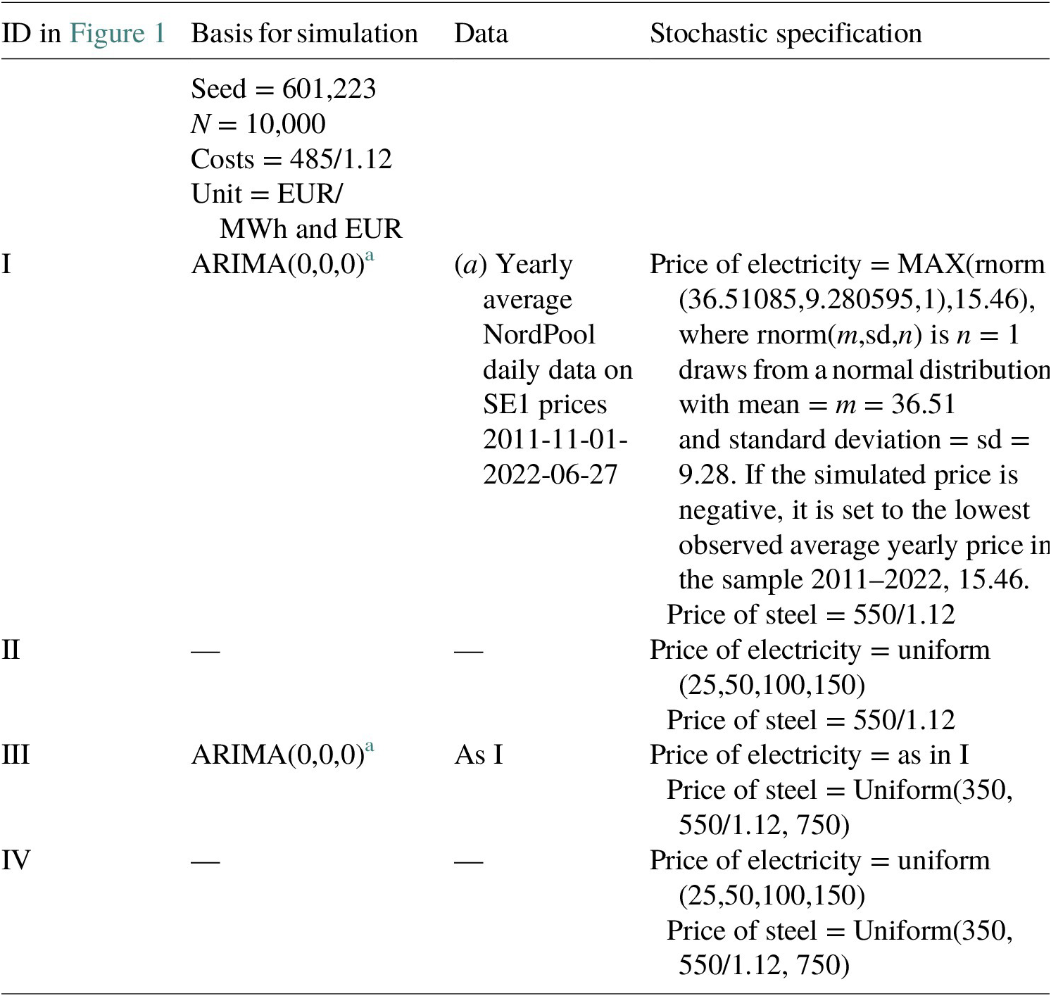
The purpose of this paper is to briefly address the question what price premium, if any, green steelmaking requires to break even. We begin in Section 2 by looking at a hypothetical existing green steelmaker that displaces production in a coal-based steel plant. Then, in Section 3, we turn to a simple investment analysis of a new plant. This analysis must be provisional because there is no existing green steel plant. The example we refer to in our evaluations is a planned plant by a company named H2 Green Steel to be located in the northern Swedish city of Boden. It is expected to be operational in 2025 and to produce 5 million tons of steel as it reaches full capacity in 2030. Almost all other data, except some prices, are taken from Koch Blank (Reference Koch Blank2019).
In Section 4, we undertake a sensitivity analysis, by computing the cost-benefit acceptability curve (see Johansson & Kriström, Reference Johansson and Kriström2016). The basic idea is to compute NPV for a given stochastic specification of the uncertain parameters. This allows us to estimate the survival function for NPV and hence the probability that the project is profitable. This systematic sensitivity analysis is more general than the standard sensitivity analysis because the latter is a special case of the former.
A few concluding remarks are added in Section 5, and an Appendix adds some details to simplify replications of our sensitivity analysis.
2. A marginal shift to green steel
Let us consider a simplified production function for green steel: iron ore, electricity, and labor are used as inputs. We focus on a marginal increase of steel, assuming a perfect market economy. Then, the WTP for the small increase equals the change in profits dπ 1:
 $$ d{\pi}_1\hskip0.35em =\hskip0.35em {dCV}_1\hskip0.5em =\hskip0.5em {p}_1{dx}_1-{p}_{io}{dq}_{io}-{p}_e{dq}_e- wdL, $$
where dCV 1 denotes the marginal compensating variation,Footnote 4 p 1 denotes the unit price of green steel, pio denotes the unit price of iron ore, pe denotes the unit price of electricity, and w denotes the labor cost per employee.
We do not have data to directly estimate Equation (1). Therefore, suppose that the alternative is to produce conventional steel within the EEA, that is, where there is a cap-and-trade system for emissions of greenhouse gases. All affected markets are assumed to be competitive. For the small or marginal alternative displaced by the green steel producer, we assume that the following holds:
 $$ {dCV}_2\hskip0.5em =\hskip0.5em {p}_2{dx}_2-{p}_{io}{dq}_{io}-\left({p}_c+{p}_p\cdot \alpha \right){dq}_c- wdL\hskip0.35em =\hskip0.35em 0, $$
where p 2 denotes the unit price of conventional steel, pc denotes the unit price of coking coal, pp denotes the price of an EU ETS permit, α converts a unit of coal to a unit of CO2, and the two considered plants are assumed to be equally labor-intensive on the margin. The maintained assumption is that the firm maximizes profits so that, at the optimum, the marginal revenue equals the marginal cost. Thus, we assume that a small adjustment of the level of production results in a zero loss of profits. This assumption will turn out to be pivotal in reformulating Equation (1).
Note that total emissions of greenhouse gases remain unchanged if the “supply” of permits is exogenous; the permits not needed by the displaced steel producer will be acquired by other users, implying that emissions are simply reshuffled.Footnote 5 For this reason, one would expect that p 1 = p 2. However, possibly due to a CO2-illusion producers and their customers (e.g., in the car and truck industries) of green steel as well as end-users expect to receive/pay a price premium, that is, p 1 > p 2. But the question is how long this illusion will last among end-users.
Deducting (2) from (1) and dividing by dx 1 (=dx 2) to obtain a measure per ton of steel yields:
 $$ {dCV}^x\hskip0.35em =\hskip0.35em {dCV}_1^x-{dCV}_2^x\hskip0.35em =\hskip0.35em \left({p}_1-{p}_2\right)-{p}_e{dq}_e^x+\left({p}_c+{p}_p\cdot \alpha \right){dq}_c^x, $$
where a superscript x refers to “per unit of output,” and $ {dCV}^x\hskip0.35em =\hskip0.35em {dCV}_1^x $
because
$ {dCV}^x\hskip0.35em =\hskip0.35em {dCV}_1^x $
because $ {dCV}_2^x\hskip0.35em =\hskip0.35em 0 $
.
$ {dCV}_2^x\hskip0.35em =\hskip0.35em 0 $
.
In order for the green steel plant to be competitive, it must be the case that dCVx > 0. Any difference $ {p}_1-{p}_2 $
reflects a price premium, that is, a WTP more for green steel. In the absence of such a premium, the shift will be profitable if the cost for electricity per unit of output falls short of avoided unit costs for coking coal and permits.
$ {p}_1-{p}_2 $
reflects a price premium, that is, a WTP more for green steel. In the absence of such a premium, the shift will be profitable if the cost for electricity per unit of output falls short of avoided unit costs for coking coal and permits.
Based on Koch Blank (Reference Koch Blank2019) a rough approximation of Equation (3), except for any price premium, is as follows:
 $$ {dCV}^x\hskip0.35em =\hskip0.35em {p}_1-{p}_2-81.25\cdot 3.45+\left(100+10\cdot 2.2\right)\cdot 0.77\hskip0.35em =\hskip0.35em \Delta p-186, $$
where $ \Delta p\hskip0.35em =\hskip0.35em {p}_1-{p}_2 $
, the electricity price, excluding transmission, is assumed to be EUR 81.25 per MWh, the price of a ton of coking coal is set to EUR 100, and the permit price is assumed to have been EUR 10 in 2018. The electricity price is the average price in one of the simulation exercises reported in the sensitivity analysis in Section 4.
$ \Delta p\hskip0.35em =\hskip0.35em {p}_1-{p}_2 $
, the electricity price, excluding transmission, is assumed to be EUR 81.25 per MWh, the price of a ton of coking coal is set to EUR 100, and the permit price is assumed to have been EUR 10 in 2018. The electricity price is the average price in one of the simulation exercises reported in the sensitivity analysis in Section 4.
If the market price of a ton of steel is EUR 490 (based on USD 550 in Koch Blank (Reference Koch Blank2019), assuming EUR 1 = USD 1.12), the price premium must be around 51 % for the green steel to be competitive.
If the green steelmaker displaces a plant outside the EEA, emissions of greenhouse gases are expected to decrease. If the global marginal damage cost of such gases exceeds EUR 10 per ton, that is, the permit price, the green steel plant will be attributed a further benefit. For example, if the marginal damage cost amounts to EUR $ 80-100 $
per ton CO2, one would add EUR
$ 80-100 $
per ton CO2, one would add EUR $ 120-150 $
to the cost-benefit analysis.Footnote
6 This might also be indicative of the benefits of switching to green steel in the US which is lacking a permit scheme for greenhouse gases.
$ 120-150 $
to the cost-benefit analysis.Footnote
6 This might also be indicative of the benefits of switching to green steel in the US which is lacking a permit scheme for greenhouse gases.
The electricity price is critical for the outcome in Equation (4). The average price over the period 2011–2022 is EUR 36.5 (and more details about the electricity price are in Section 4). Then, the loss per ton of steel, exclusive of any price premium and any real transmission costs, reduces to EUR 32.
If the electricity price (including any social costs for transmission of electricity) is reduced to EUR 27 per MWh, $ {dCV}^x\hskip0.35em =\hskip0.35em \Delta p $
. That is, green steel breaks even also in the absence of any price premium. However, if the plant produces 5 million tons annually, according to Equation (4) it will consume more than 17 TWh per year. There are several other planned electricity-consuming plants in the region – the counties of Norrbotten and Västerbotten in northern Sweden – such as another green steelmaker and the battery producer Northvolt. Together, these new users are expected to demand 85–90 TWh annually.Footnote
7 This is roughly half of Sweden’s electricity production. It is hard to see how this will be possible without causing dramatic price increases. Even if electricity can be imported via the Nordic Nord Pool market, there are bottlenecks; transmission capacity is simply limited, and the lead times of transmission line expansions are long. Probably, the projects necessitate costly expansions of the transmission network. The more densely populated southern parts of Sweden have experienced electricity prices of more than EUR 200 per MWh. These considerations motivate the quite high electricity price in Equation (4).
$ {dCV}^x\hskip0.35em =\hskip0.35em \Delta p $
. That is, green steel breaks even also in the absence of any price premium. However, if the plant produces 5 million tons annually, according to Equation (4) it will consume more than 17 TWh per year. There are several other planned electricity-consuming plants in the region – the counties of Norrbotten and Västerbotten in northern Sweden – such as another green steelmaker and the battery producer Northvolt. Together, these new users are expected to demand 85–90 TWh annually.Footnote
7 This is roughly half of Sweden’s electricity production. It is hard to see how this will be possible without causing dramatic price increases. Even if electricity can be imported via the Nordic Nord Pool market, there are bottlenecks; transmission capacity is simply limited, and the lead times of transmission line expansions are long. Probably, the projects necessitate costly expansions of the transmission network. The more densely populated southern parts of Sweden have experienced electricity prices of more than EUR 200 per MWh. These considerations motivate the quite high electricity price in Equation (4).
A benefit for society not accounted for thus far occurs if the considered steelmaker causes (regional) unemployment to decrease, either directly or indirectly via subcontractors and services. However, the region is already in short supply of labor due to the high demand from green start-up plants, and firms are looking “all over the world” to find laborers.
The involved prices have been relatively stable over long periods of time. However, recently prices have been volatile and there have been sharp increases in p 2, pc, and pp, possibly due to the pandemic, Russia’s assault on Ukraine, distortions in supply chains, inflationary pressures, and, in the case of pp, also a reform of the EU ETS. We have no detailed price data, but the sign of Equation (4) is reversed if the updated prices in Section 3 are used (and pp is set equal to EUR 80). However, it is hard to say if these high and volatile prices will persist when we (hopefully) return to more normal times. In any case, we need an investment appraisal in order to say whether investing in green steel is profitable to society. We now turn to an outline of such an appraisal.
3. A sketch of an investment appraisal
A simple way of checking whether Equation (4) provides a reasonable estimate would be to undertake an investment appraisal of a green steel plant. However, to the best of our knowledge, there are no detailed data available. Therefore, we continue to draw on Koch Blank (Reference Koch Blank2019).
The provisional investment appraisal is summarized in Equation (5). The plant is assumed to produce 5 million tons of steel annually, and the time horizon is set to 20 years. We continue to use EUR 550/1.12 as the market price of “conventional” steel, and the exchange rate between USD and EUR is around 1.12 in 2019. According to Koch Blank (Reference Koch Blank2019) the cost of producing a ton of green steel, exclusive of the electricity cost, is EUR 485/1.12. The cost of an MWh electricity is once again assumed to be EUR 81.25, and the social discount rate is set equal to 3 %.Footnote 8 In the absence of a price premium, the net present value (NPV) of the investment equals:
 $$ NPV\hskip0.35em =\hskip0.35em {\sum}_{t\hskip0.35em =\hskip0.35em 1}^{20}\left(\frac{550}{1.12}-\frac{485}{1.12}-81.25\cdot 3.85\right)\cdot 5\cdot {10}^6\cdot {1.03}^{-t}\hskip0.35em =\hskip0.35em -\hskip-0.55em 16.5\cdot {10}^9. $$
In the absence of a price premium, the loss is huge. To break even, the price premium would have to be over 45 %; doubling the social discount rate to 6 % leaves the price premium unchanged. If the electricity price is reduced to EUR 36.5, the loss reduces to around EUR 5 billion (109), and break even then requires a price premium of almost 14 %. Alternatively, without a price premium, the NPV in Equation (5) would equal zero if the electricity price, including any real transmission cost, is reduced to just below EUR 17 per MWh.
A rough update of prices to 2022 levels yields p
2 ≈ 650, and pio ≈ 125.Footnote
9 Typically, it takes 1.6 tons of iron ore to produce 1 ton of crude iron.Footnote
10 Using the new crude steel price in Equation (5) and adding $ 1.6\cdot \left(125-60\right) $
to costs in the equation reduces the present value loss by around EUR 4.5 billion.
$ 1.6\cdot \left(125-60\right) $
to costs in the equation reduces the present value loss by around EUR 4.5 billion.
The maintained assumption has been that the plant displaces steel production within the area covered by the EU ETS; for example, it will compete directly with the Swedish steel manufacturer SSAB’s plant in Domnarvet (in Sweden). However, if production is displaced at a location not covered by any CO2-policy, one would have to add net present benefits amounting to some EUR $ 10-13 $
billion if the global marginal damage cost equals EUR
$ 10-13 $
billion if the global marginal damage cost equals EUR $ 80-100 $
per ton CO2. Thus, if the electricity price remains around EUR 36.5 per MWh, the switch to green or fossil-free steel might be socially profitable. The same seems likely to hold true also for a plant operating in the US.
$ 80-100 $
per ton CO2. Thus, if the electricity price remains around EUR 36.5 per MWh, the switch to green or fossil-free steel might be socially profitable. The same seems likely to hold true also for a plant operating in the US.
Overall, the investment appraisal results in a more negative picture than the marginal analysis of a plant assumed to already be operational. However, it is hardly surprising that the two approaches result in different outcomes. For example, even if there is an interior solution such that dCV = 0 in Equation (4), the plant could earn a positive or negative overall profit.
4. Systematic sensitivity analysis
In this section, we undertake a sensitivity analysis, by computing the cost-benefit acceptability curve (see Johansson & Kriström, Reference Johansson and Kriström2016). The basic idea is to compute NPV for a given stochastic specification of the uncertain parameters. This allows us to estimate the survival function for NPV and hence the probability that the project is profitable. This systematic sensitivity analysis is more general than the standard sensitivity analysis because the latter is a special case of the former.
The electricity price is particularly important for the investment appraisal, and we have therefore used several different approaches to the modeling of expected future electricity prices. The first uses ARIMA models on Nord Pool spot price data (2011–2022) for price area SE1, that is, the northernmost of Sweden’s four electricity price areas, where the plant under consideration is to be located. Producers of electricity in SE1 and SE2 are (virtually always) net exporters. This is mainly because a significant part of Sweden’s hydropower capacity is located in SE1 and SE2, while roughly 9/10 of the population lives in SE3 + SE4.
The electricity prices in SE1 and SE2 are generally lower than those found in SE3 and SE4, because of transmission constraints. The price differences have been significant during 2021 and 2022, with prices in the south being up to 1 000 per cent higher than those in the north. While electricity prices in SE1 + SE2 have remained relatively low (about EUR 36 per MWh, 2011–2022 average), prices in the south of Sweden have reached unprecedented levels in the summer of 2022 (more than EUR 200 per MWh). Figure 1 summarizes the key development of electricity prices.
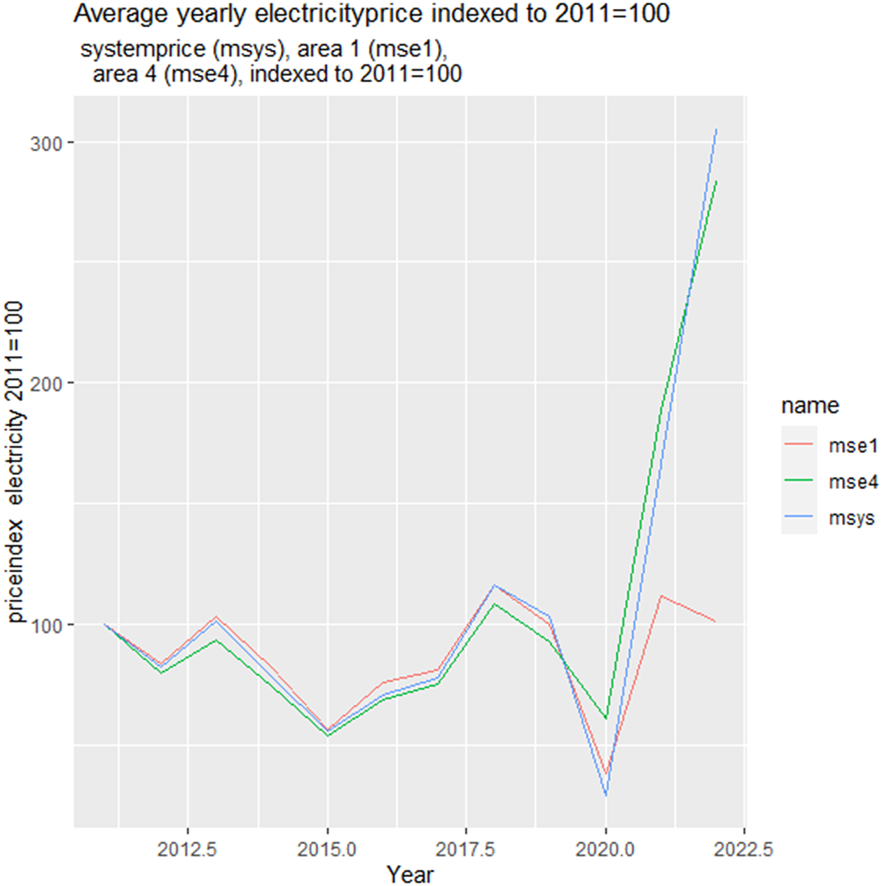
Figure 1. Electricity prices indexed to 2011 = 100 on Nord Pool. mse1, average yearly price in price area 1; mse4, average yearly electricity price in price area 4, msys, average yearly system price.
Figure 1 shows that average yearly electricity prices were generally similar on the Nord Pool up to 2020. Prices in SE2 and SE3 are not shown, because they follow closely the pattern in Figure 1, with SE2 (SE3) tracking SE1 (SE4) prices closely. At the yearly average level, area prices are very similar to Nord Pool’s system price (i.e., the market price that would result without transmission constraints). The unusually low average price in 2020 is followed by increases in SE4 and the system price in 2021 and 2022 (up to 2022-06-27). The average yearly price in 2022 has turned down in SE1. Note that the price in SE1 is about the same in 2022 as in 2011, while the price in SE4 is about three times higher than the average yearly SE4 price in 2011.
The electricity price of relevance to the investment considered here is the price prevailing locally, currently the price in SE1. The significant price differences between north and south have led to a discussion about the usefulness of the current price area configurations; an abolishment of the price areas would equalize the price across Sweden, benefitting consumers in SE3/SE4 and producers in SE1/SE2. There has also been a discussion about the merits of exporting electricity from north to south; the electricity “is needed” (it is claimed in the north, given the planned industrial expansions). As far as we can tell, the price areas will remain in the near future.
It is difficult to predict the combined effects of the expected increase of domestic demand and supply on the future electricity price, let alone any change of the price areas. Such a forecast must also consider the ongoing Europeanisation of the electricity market, which essentially means that the invariably cheaper electricity in Northern Europe will become more easily accessible for the markets in Southern Europe. There are also several reasons as to why the average yearly prices we use here are higher than those actually faced by the firm. First, official statistics on historical electricity prices on Nord Pool shows that the larger the installed effect, the lower the price.Footnote 11 Secondly, it is possible that the firm enters into a bilateral contract off Nord Pool, should the terms be more favorable. Nevertheless, if the considered plant has market power in the electricity market, from a societal point of view the relevant price still is the marginal one in the market. There are other, fanciful future possibilities, involving the construction of small modular reactors (SMRs) close to the green steel plant.
Given the significant uncertainty about the electricity prices in the coming 20 years, we proceed in two different ways when specifying the electricity price distribution: an ARIMA time-series analysis and an ad hoc specification, containing our “best guess” on the future electricity price distribution.
The ARIMA analysis on the price data for SE1 2011-11-01-2022-06-27 shows that the best-fitting model is of the form ARIMA(0,0,0). This result provides some support for our use of the normal distribution with a constant mean as a basis for the first group of simulations, although it makes the strong assumption that the variance is constant. Furthermore, while the electricity price has been observed to be negative some hours on the Nord Pool market, it can certainly not be negative on the average over a whole year. Rather than using a transformation or a distribution with positive support, we simply replace any negative draw with the lowest observed average price in SE1 during 2011–2022.
An analysis of the residuals from the ARIMA models, suggests that the model for the system price does not work well in the tails (as may be expected when considering Figure 1). The variance of the residuals from this ARIMA model appears not to be constant, rather strongly increasing (using the methodology outlined in Tsay, Reference Tsay1988). The increasing future share of intermittent electricity generation sources suggests that the price will be more variable and hence that our assumption of a constant normal distribution through time is questionable. But given the projected changes in the electricity market described above, this stochastic specification can be regarded as a kind of lower bound. The second stochastic specification reflects our belief that the future electricity price is unlikely to be lower (higher) than EUR 25 (150) as a yearly average. Because of the difficulty of providing estimates of the probabilities, we assume a uniform distribution in this case.
The ARIMA approach thus motivates us to use a normal distribution with a mean of about EUR 36 (and a standard deviation of about 9), while we in the second approach apply a uniform distribution over (25,50,100,150), which implies a mean price of EUR 81.25 and a standard deviation of about 48. The specifics of our simulations are listed in the Appendix. The seed used can be employed for replicating the simulation in R.
The results are summed up in Figure 2. Panels I and III refer to the ARIMA approach while panels II and IV refer to our second approach. The curves represent survival functions. We have marked the median in each of the panels. These simulations suggest that the present value is unlikely to be positive, although it can happen if the combination of electricity and steel prices is particularly benign.
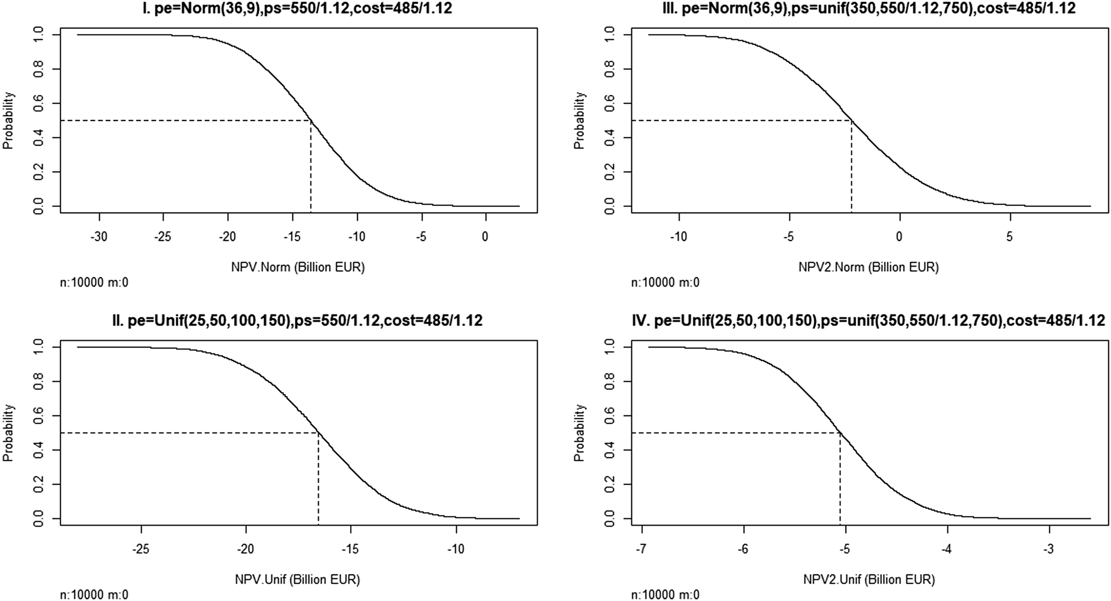
Figure 2. Sensitivity analysis. Acceptability curves for net present value of investment (r = 0.03, N = 20 years). cost, unit cost of production (EUR); pe, price of electricity (EUR/MWh); ps, price of steel (EUR).
5. Concluding remarks
Steelmaking is one of the larger emitters of greenhouse gases. Therefore, it is essential to bring down the steel industry’s emissions in order to reach the Paris Agreement.Footnote 12 High expectations are placed on green or fossil-free steelmaking. The problem is that such steelmaking requires huge amounts of electricity. In the case under consideration, the problem is multiplied manyfold due to a number of spectacular “green” start-ups located within a relatively small and sparsely populated region. Together these new plants are expected to consume around half of Sweden’s electricity production. It is hard to see how such a huge expansion of demand is possible to meet without price increases.
The good news is that green steelmaking could become competitive in locations with low electricity prices. Thus, the results of this paper do not suggest that green steel represents a dead end.
Acknowledgment
Financial support from the Swedish Agency for Growth Policy Analysis and MISTRA Electrification is gratefully acknowledged.
Competing Interests
The authors declare none.
A. Appendix


 Open access