Gender norm conflict and marital outcomes

Francisca M. Antman; Priti Kalsi; Soohyung Lee

doi:10.1017/dem.2021.7

Gender norm conflict and marital outcomes

Published online by Cambridge University Press: 25 March 2021

Francisca M. Antman

Priti Kalsi and

Soohyung Lee

Show author details

Francisca M. Antman*: Affiliation:
Department of Economics, University of Colorado Boulder, 256 UCB, Boulder, CO80309, USA IZA, Institute of Labor Economics, Bonn, Germany
Priti Kalsi: Affiliation:
Department of Economics, Rochester Institute of Technology, 92 Lomb Memorial Drive, Rochester, NY14623, USA
Soohyung Lee: Affiliation:
IZA, Institute of Labor Economics, Bonn, Germany Graduate School of International Studies, Seoul National University, Seoul08826, South Korea
*: *Corresponding author. E-mail: francisca.antman@colorado.edu

Article contents

Abstract
Introduction
Conceptual framework
Data and descriptive statistics
Empirical strategy
Results
Conclusion
Footnotes
References

Abstract

We investigate the impact of male–female conflict over gender norms on marital outcomes. As marriage requires mutual agreement regarding the role of husband and wife, we hypothesize that a person who is less likely to encounter a potential mate with similar gender norms will face a lower chance of marrying. Even if two parties marry despite a difference in gender norms, their marriage may be more vulnerable to external shocks, making divorce more likely relative to their counterparts without gender norm conflict. Finally, we predict that in the presence of gender norm conflict, high-skilled individuals may be less likely to get or stay married relative to low-skilled individuals, as the former group faces better outside options. Estimates from an analysis of U.S. marriage markets differentiated by birth cohort, state, race, and skill level support our theoretical predictions. Additional extensions explore heterogeneous effects and additional outcomes such as the presence of children in the household.

Keywords

Divorce gender marriage skill gap social norms

JEL classification

J12: Marriage • Marital Dissolution • Family Structure • Domestic Abuse J24: Human Capital • Skills • Occupational Choice • Labor Productivity J16: Economics of Gender • Non-labor Discrimination

Type: Research Paper
Information: Journal of Demographic Economics , Volume 87 , Issue 4 , December 2021 , pp. 537 - 560

DOI: https://doi.org/10.1017/dem.2021.7 [Opens in a new window]
Creative Commons: This is an Open Access article, distributed under the terms of the Creative Commons Attribution licence (http://creativecommons.org/licenses/by/4.0/), which permits unrestricted re-use, distribution, and reproduction in any medium, provided the original work is properly cited.
Copyright: Copyright © Université catholique de Louvain 2021

1. Introduction

One of the most striking demographic changes in the United States in recent years has been the well-documented decline in marriage rates across cohorts over time. While several explanations have been offered for this phenomenon, one of the more salient economic rationales is rooted in increased opportunities for women which have themselves been facilitated by changing norms surrounding the role of men and women in society [Bertrand et al. (Reference Bertrand, Cortes, Olivetti and Pan2018)]. We build on this literature by exploring an innovative view of gender conflict that measures disagreement over the roles of men and women within marriage. Intuitively, disagreement over spousal roles within marriage should affect each party's net gains from marriage and therefore affect marital outcomes. Thus, we ask: To what extent can dissimilar notions of marriage between men and women, as measured by the probability of agreement with a traditional view of gender roles, explain variation in marriage and divorce rates across groups?

To address this question, we set up a simple model closely following Bertrand et al. (Reference Bertrand, Cortes, Olivetti and Pan2018) where gender norms help to determine the net benefit of marriage over and above remaining single, individuals are matched randomly within marriage markets, and gender norms are exogenously given. As in Bertrand et al. (Reference Bertrand, Cortes, Olivetti and Pan2018), our model presumes that traditional notions surrounding a woman's role in the home limit the benefit that traditional men gain from marriage because a traditional man places little value on his spouse's career. Unlike Bertrand et al. (Reference Bertrand, Cortes, Olivetti and Pan2018), however, we also incorporate gender norms into the value of singlehood. Specifically, in our model, traditional women perceive a social penalty to remaining single, and thus prefer to marry, all else equal, relative to women with more modern gender norms. In a static model of a marriage market with a simple random match, it follows that the match between a man with a traditional gender norm and a woman with a modern gender norm yields the lowest probability of marriage. Consequently, we should observe lower marriage rates in marriage markets with a higher share of traditional men and modern women all else equal, and we investigate this prediction empirically.

The intuitive spirit of our result is that marital happiness is likely to be lower when there are conflicting gender norms between potential mates, and thus we should expect marriage rates to be lower when a person is less likely to encounter a partner with similar views on the roles of men and women within marriage. Moreover, even if two parties temporarily overlook their differences and become married, we expect they will face a greater likelihood of divorce in the event of negative external shocks if there exists a fundamental disagreement over gender norms. Finally, we expect that the marital choices of skilled individuals, who face better labor market opportunities outside of marriage, will be more responsive to gender norm conflict compared with their unskilled peers.

We find evidence to support our predictions using demographic data on U.S. marriage markets covering cohorts born between 1920 and 1979 drawn from the American Community Survey matched with data on gender norms held by men and women in those markets drawn from the General Social Survey. In particular, we show that the disagreement in gender norms is negatively correlated with the marriage rates in marriage market groupings defined by state, race, skill, and birth cohort, and positively correlated with divorce rates. Further extensions explore heterogeneity by race and by the extent of gender norm conflict in a marriage market, as well as the impact of gender norm conflict on marriage quality and marital investments, as proxied by the presence of children. Throughout the paper, we take gender norms as exogenously given, which is the standard in the literature on this topic. However, it is important to note that attitudes toward marriage and divorce may be correlated with attitudes toward the gendered division of labor for unobserved reasons that we do not explore here. Thus, we emphasize that this paper only seeks to establish a correlation and suggest a model that could explain the association between marital outcomes and gender norms. In that sense, it constitutes a first descriptive step in the larger effort to causally link these two important phenomena.

This paper adds to a growing literature suggesting that gender norms play an important role in determining the economic outcomes of individuals and their descendants. For example, studies have examined attitudes toward women's labor market participation [e.g., Farré and Vella (Reference Farré and Vella2012)], willingness to have a working wife [e.g., Fernandez et al. (Reference Fernandez, Fogli and Olivetti2004)], and the gendered division of household work [e.g., Sevilla-Sanz (Reference Sevilla-Sanz2010); Giménez-Nadal et al. (Reference Giménez-Nadal, Mangiavacchi and Piccoli2012); Giménez-Nadal et al. (Reference Giménez-Nadal, Molina and Sevilla-Sanz2019)], in addition to marital outcomes within and across countries, such as the rise in cross-border marriages [Kawaguchi and Lee (Reference Kawaguchi and Lee2016)]. Alesina et al. (Reference Alesina, Giuliano and Nunn2013) suggest gender role differences across cultures are especially persistent and may even follow immigrants to their new destinations. More broadly, our work is connected to the wider literature on the economics of the family that studies the link between marriage rates and the relative gains to marriage [Choo and Siow (Reference Choo and Siow2006)]. While the literature on gender norms does not generally distinguish between gender norms for men and women separately, our model incorporates heterogeneity in gender norms across sexes and thus allows for the possibility of mismatch in gender norms between a randomly matched man and woman.Footnote ¹ Thus, our work complements the literature in family economics by showing how gender norm conflict between men and women may also explain marital outcomes.

The paper proceeds as follows. Section 2 describes the conceptual framework which motivates the empirical prediction regarding the impact of gender norms on marriage rates, as well as other intuitive results. Section 3 describes the data used to link marriage rates with views on traditional gender norms and presents summary statistics. Section 4 describes the empirical strategy and presents the main estimating equation. Section 5 discusses the main results and extensions. Section 6 concludes.

2. Conceptual framework

2.1 Background and intuition

To motivate our predictions, we set up a simple model that follows the literature incorporating gender norms and the marital division of labor into formal models of marriage formation [Fernandez et al. (Reference Fernandez, Fogli and Olivetti2004), Bertrand et al. (Reference Bertrand, Cortes, Olivetti and Pan2015, Reference Bertrand, Cortes, Olivetti and Pan2018), Kawaguchi and Lee (Reference Kawaguchi and Lee2016)]. In particular, we modify the static model of marriage and household decision-making used in Bertrand et al. (Reference Bertrand, Cortes, Olivetti and Pan2018) to illustrate the implications of men and women having different views on gender roles with respect to marriage rates. Our model follows closely from Bertrand et al. (Reference Bertrand, Cortes, Olivetti and Pan2018) in assuming that gender norms held by men and women directly affect the gains from marriage through the value of a spouse's earnings on individual utility. We extend a simplified version of their model by assuming that gender norms also affect the value of singlehood by means of conferring a social stigma on women with traditional gender norms who remain single. Thus, while Bertrand et al. (Reference Bertrand, Cortes, Olivetti and Pan2018) focus on the impact of gender norms on the skilled-unskilled marriage gap, we focus on the impact of gender norm disagreement in marriage markets on marital outcomes. As in Bertrand et al. (Reference Bertrand, Cortes, Olivetti and Pan2018), we take gender norms as exogenously given.

For simplicity, we consider marriage as a union between a man and a woman, formed only if both parties jointly prefer marriage to remaining single. As is standard in the literature, we assume that the married household makes decisions by maximizing a weighted sum of the husband's and wife's utilities from marriage, where the weight is exogenously given and lies strictly between 0 and 1. Each person's utility depends on the consumption of market goods and the outcome of home production. By assumption, the latter is a public good, thus allowing for the possibility that marriages may constitute a Pareto-improvement over both parties remaining single.

In this setting, the net benefit of a marriage depends not only on the characteristics of two individuals but also on the gender norms which influence the division of labor in the market and at home for men and women. For simplicity, we can characterize the gender norms into two broad categories: modern and traditional. At the extreme, a traditional man places no value on his wife's wages and a traditional woman would rather marry any man than remain single. In contrast, modern men and women make marital decisions that take the wages of both parties into account. These assumptions imply that, all else equal, a modern woman is less likely than a traditional woman to find a traditional man acceptable for marriage. While these extreme cases are purely to develop intuition, one can see how the model suggests that the marriage rate will be lower in a market with a higher probability of a random meeting between a traditional man and a modern woman, that is, in markets with a higher rate of interaction between the share of men with traditional norms and women with modern norms. Thus, the main contribution of the model is to show that when there are groups of men and women that gain less from marriage due to conflicting gender norms, the greater the share of these people in a given marriage market, the lower the resulting marriage rates will be in that market.Footnote ²

2.2 Setup

2.2.1 Value of marriage

In this model, agents are endowed with one unit of time, which can be spent producing a market good, or a household public good if the agents marry. Man m's utility from marrying woman w depends on four components: the utility from his own private consumption, utility from consuming a household public good, a spillover effect from his spousal private consumption, and a random shock drawn from the standard normal distribution (q _m). Woman w's utility from that marriage is defined likewise, where we note that the random shock (q _w) is drawn independently from that of man m's.Footnote ³

Man m's private consumption is assumed to be the product of the wage rate (w _m) and time spent on market production (1 − t _m). A household good depends on the sum of m's and w's household production. Specifically, man m's utility from marrying woman w and woman w's utility from marrying man m are as follows:

$$\eqalign{V_m( {w_m, \;\;w_w, \;q_m} ) = & ( {1-t_m} ) w_m + \alpha _m( {1-t_w} ) w_w + \beta \ln ( {t_m + t_w} ) + q_m, \;\cr V_w( {w_m, \;\;w_w, \;q_w} ) = & ( {1-t_w} ) w_w + \alpha _w( {1-t_m} ) w_m + \beta \ln ( {t_m + t_w} ) + q_w, \;} $$

where t _m, t _w ∈ [0, 1], and β > 0.Footnote ⁴

Parameters α _m and α _w measure the extent to which each agent gets utility from the spouse's private consumption. We follow Bertrand et al. (Reference Bertrand, Cortes, Olivetti and Pan2018), in setting α _w to be 1 and using α _m to measure the extent to which men are traditional, a value that ranges between 0 and 1 in Bertrand et al. (Reference Bertrand, Cortes, Olivetti and Pan2018).

Justifying this approach, Bertrand et al. (Reference Bertrand, Kamenica and Pan2016) offer one interpretation for the utility function as one in which an individual derives utility from his/her own career and his/her spouse's career “in a way that is proportional to its status or success as measured by wages” (p. 12). Thus, a low value of α _m indicates whether a man has a traditional gender norm, i.e., he derives little social status from her career. As Bertrand et al. (Reference Bertrand, Kamenica and Pan2016) emphasize, “This parameter captures the idea that a working/career wife might challenge the conventional idea of gender roles in a household [e.g., “identity” as in Akerlof and Kranton (Reference Akerlof and Kranton2000)]” (p. 12).

For simplicity, we set α _m to be either 0 or 1, where α _m = 0 describes men with the traditional gender norm while α _m = 1 describes men who do not have the traditional gender norm. Note that by setting α _m = 1, men have the same utility function as women, thus incorporating gender equality (symmetry).Footnote ⁵ This simplifying assumption on α _m allows us to obtain a set of closed-form solutions which highlight the impact of gender norm conflict on marriage rates.

Once a marriage is formed, the couple jointly decides the time spent for home production (t _m, t _w) by maximizing γV _m(w _m, w _w, q _m) + (1 − γ)V _w(w _m, w _w, q _w) where 0 < γ < 1. Under this unitary model of household decision-making, if w _m > w _w > β, then the optimal choices of time allocation are t _m = 0 and t _w = β/w _w.

2.2.2 Value of singlehood

An important distinction between our model and that in Bertrand et al. (Reference Bertrand, Cortes, Olivetti and Pan2018) is in the value of singlehood. Whereas Bertrand et al. (Reference Bertrand, Cortes, Olivetti and Pan2018) assume the value of singlehood depends only on a person's own wage, in our model, it depends on both the wage and stigma associated with singlehood, which varies by gender norms. Specifically, we assume that the utility from being single is the sum of the wage rate (w) and the extent to which a person thinks that not being married carries a social cost (θ):

$$V_{{\rm single}} = w-\theta .$$

If a person has θ = 0, he/she does not think there is a particular stigma to remaining single in society while if θ is positive, being single could lead to stigma or social costs (e.g., being socially marginalized). For simplicity, we set the value of θ for men at zero to act as a baseline. For women, we assume that if a woman has a traditional gender norm, she has a positive value of θ but if she does not, the value of θ is equal to zero, the same as for men.

2.3 Marriage market

As in Bertrand et al. (Reference Bertrand, Cortes, Olivetti and Pan2018), we consider a static marriage market in which agents are randomly matched to another agent from the opposite sex out of the pool of singles. A household is formed if and only if both man and woman in a matched couple both prefer marriage to remaining single. It is worth noting two features of our model. First, due to the static nature of the model, agents do not accept/reject a marriage opportunity with the expectation of any future marriage opportunity (i.e., option value). This helps us to derive a closed-form solution. Second, our model follows a set of existing studies using non-transferable utility frameworks in modeling marriage decisions [e.g., Smith (Reference Smith2006)]. Unlike models based on Becker (Reference Becker1973), these frameworks do not allow monetary transfers between two individuals prior to marriage in order to transfer some of the net gains from marriage.

To highlight the interaction between the gender norm and marriage, we focus on the setting where w _m > w _w > β, in which the optimal choices of time allocation are t _m = 0 and t _w = β/w _w. If man m and woman w are matched to each other, both will agree to get married if and only if the following two conditions hold:

$$q_m \ge q_m^\ast \equiv -1 \times \{ {\alpha_m( {w_w-\beta } ) + c{\rm \, }} \} , $$

and

$$q_w \ge q_w^\ast \equiv -1 \times \{ {w_m-\beta + \theta + c} \} , \;$$

where c = βln(β/w _w). Thus, man m and woman w will agree to marry each other if and only if $q_m \ge q_m^\ast$ and $q_w \ge q_w^\ast$. Therefore, we can examine the impact of gender norm conflict on marriage rates by studying the relationship among the four variables: α _m, θ, $q_m^\ast$, and $q_w^\ast$.

Man m's reservation match quality is:

$$q_m^\ast ( {{\rm traditional}} ) = {-}c\,{\rm if}\,{\rm he}\,{\rm holds}\,{\rm the}\,{\rm traditional}\,{\rm norm, \;}$$

$$q_m^\ast ( {{\rm modern}} ) = {-}( {w_w-\beta } ) -c\,{\rm if}\,{\rm he}\,{\rm holds}\,{\rm the}\,{\rm modern}\,{\rm norm} .$$

Woman w's reservation match quality is

$$q_w^\ast ( {{\rm traditional}} ) = {-}w_m + \beta -\theta -c\,{\rm if}\,{\rm she}\,{\rm holds}\,{\rm the}\,{\rm traditional}\,{\rm norm}\,( {\rm with}\,\theta > 0) , \;$$

$$q_w^\ast ( {{\rm modern}} ) = {-}\;w_m + \beta -c\,{\rm \;if}\,{\rm she}\,{\rm holds}\,{\rm the}\,{\rm modern}\,{\rm norm}.$$

Therefore, we can formulate the probability of man m and woman w getting married to each other depending on their gender norms as shown in Table 1.

Table 1. Gender norms and probability of marriage for men and women

Note: Φ refers to the c.d.f. of the standard normal distribution.

2.4 Theoretical implications

2.4.1 Main results

Table 1 shows the likelihood of marriage occurring between traditional and modern men and traditional and modern women, respectively, i.e., the probability that both man and woman exceed their reservation thresholds for match quality and form a union. Specifically, variable M _AB represents the likelihood of a match between man with type A gender norm (Modern, M, or Traditional, T) and woman with type B gender norm (M or T). As we assume that the random components of match quality (q _m and q _w) are i.i.d., we can calculate the likelihood as follows:

$$M_{TT}\equiv {\rm \Phi }( c ) \times {\rm \Phi }( {w_m-\beta + \theta + c} ) , \;$$

$$M_{MT}\equiv {\rm \Phi }( {c + w_w-\beta } ) \times {\rm \Phi }( {w_m-\beta + \theta + c} ) , \;$$

$$M_{TM}\equiv {\rm \Phi }( c ) \times {\rm \Phi }( {w_m-\beta + c} ) , \;$$

and

$$M_{MM}\equiv {\rm \Phi }( {c + w_w-\beta } ) \times {\rm \Phi }( {w_m-\beta + c} ) .$$

It is worth noting that in our model, the likelihood of a man and woman getting married depends on their gender norms, not because they care about the other person's gender norm explicitly, but because their gender norms affect the reservation match quality.

As all parameters, w _m, w _w, β, and θ, are positive and we focus on the case w _m > w _w > β, we can rank them:Footnote ⁶

$$M_{MT} > M_{TT}\;> M_{TM}, \;\,{\rm and} \; M_{MT} > M_{MM} > M_{TM}.$$

That is, the probability of marriage will be the lowest if a traditional man is matched with a modern woman.

We denote by p _m the share of men having a traditional norm and by p _w the share of women having a traditional norm. For example, the chance that a traditional man is matched with a modern woman within a marriage market is p _m × (1 − p _w). Then, the marriage rate of this market (M) is a weighted sum of M _TT, M _MT, M _TM, and M _MM:

$$\eqalign{M & \equiv p_mp_wM_{TT} + p_m( {1-p_w} ) M_{TM} \cr & \quad + ( {1-p_m} ) p_wM_{MT} + ( {1-p_m} ) ( {1-p_w} ) M_{MM}.} $$

Implication 1: Suppose that 0 < p _m < 1 and 0 < p _w < 1. As p _m × (1 − p _w) increases, the overall marriage rate in a market decreases.

Proof: Suppose that 0 < p _m < 1 and 0 < p _w < 1. We denote by χ = p _m × (1 − p _w). Then, we can show that dM/dχ is negative as follows:

$$\displaystyle{{dM} \over {d\chi }} = \displaystyle{{\partial M} \over {\partial p_m}}\displaystyle{{\partial p_m} \over {\partial \chi }} + \displaystyle{{\partial M} \over {\partial ( {1-p_w} ) }}\displaystyle{{\partial ( {1-p_w} ) } \over {\partial \chi }} = \displaystyle{{\partial M} \over {\partial p_m}}\displaystyle{1 \over {( {1-p_w} ) }} + \displaystyle{{\partial M} \over {\partial ( {1-p_w} ) }}\displaystyle{1 \over {\,p_m}}, \;$$

where

$$\displaystyle{{\partial M} \over {\partial p_m}} = p_w( {M_{TT}-M_{MT}} ) + ( {1-p_w} ) ( {M_{TM}-M_{MM}} ) $$

and

$$\displaystyle{{\partial M} \over {\partial ( {1-p_w} ) }} = p_m( {M_{TM}-M_{TT}} ) + ( {1-p_m} ) ( {M_{MM}-M_{MT}} ) .$$

As M _MT > M _TT > M _TM, and M _MT > M _MM > M _TM, both ∂M/∂p _m and ∂M/∂(1 − p _w) are negative, resulting in dM/dχ being negative.

In the empirical section below, we will test if Implication 1 holds in our empirical setting by examining to the extent to which our measure of gender norm conflict, p _m × (1 − p _w), is negatively correlated with marriage rates using a linear regression method. We postpone detailed discussions of the empirical model implementation to section 4 once we have explained the data used in the analysis.

2.4.2 Extensions

The simple model laid out above shows that the impact of gender norm conflict on the marriage rate depends on the following parameters: p _m, (1 − p _w), w _m, w _w, β, and θ. Thus, we can motivate empirical extensions that are intuitively linked with our simple framework.

First, we recognize that some couples may marry despite conflict over gender norms. All else being equal (i.e., w _m, w _w, q _m, q _w), our model predicts that disagreements on gender norms lower the net benefit from marriage. Therefore, we expect couples facing greater gender norm conflict will be more likely to get divorced when they are hit by negative shocks during marriage.Footnote ⁷ Moreover, divorced individuals in markets with greater gender norm conflict will be less likely to remarry, and thus further raise the share of individuals observed to be currently divorced. For this reason, we add divorce rates as an additional outcome variable throughout our empirical analysis. At the same time, it is important to highlight the fact that we do not observe the random component of the match quality (q _m, q _w), and it may be that, due to selection into marriage, the married couples with gender norm conflicts may on average have higher unobserved match qualities than their counterparts without conflicts. If true, this type of selection would mean that couples formed despite disparate gender norms would be less likely to separate when faced with shocks in subsequent periods. Thus, any empirical pattern showing a positive association between gender norm conflict and divorce rates should be interpreted as a conservative estimate of the true association between the two variables, as it would be biased downward by any positive selection into marriage. Indeed, this is what we find (see section 5.2).

In further extensions, we allow for possible heterogeneous effects of gender norm conflicts on marital outcomes due to differences in labor market opportunities, the extent of gender norm conflicts, and race. First, as wage levels of men and women affect the value of marriage and singlehood, we can examine whether marriage market outcomes vary based on outside labor market opportunities. To approximate individuals' labor market opportunities, we classify men and women into skilled and unskilled groups depending on their educational attainment. We expect that skilled individuals will be more responsive to gender norm conflict than their unskilled peers, as higher skilled individuals have better labor market opportunities, and thus face a higher outside option as unmarried individuals. For example, even a woman with modern gender norms may accept and keep a traditional man as a husband if she earns a lower wage rate, while a modern woman with better labor market opportunities might not. Thus, we expect that skilled individuals, who have better economic opportunities outside of marriage, will be less likely to marry and more likely to divorce in the face of gender norm conflict compared with their unskilled peers.

Next, we examine heterogeneous effects that vary depending on the extent of gender norm conflicts. Specifically, we distinguish marriage markets based on whether the share of modern women in a marriage market exceeds the share of traditional men. It may be worth noting that it is ambiguous whether the marriage rate in a market would be more affected by having more traditional men in the market, holding others constant, as compared to having more modern women. This is because without introducing more assumptions, we cannot determine whether ∂M/∂p _m or ∂M/∂(1 − p _w) is larger. For this reason, we examine only the role of gender norm conflicts measured by the product of p _m and (1 − p _w), instead of focusing on p _m and (1 − p _w) separately, and explore heterogeneous impacts using the interaction model laid out below.

In addition, due to preferences over homogamyFootnote ⁸, marriage markets may be partially segregated by demographic characteristics such as race, raising the possibility that gender norm conflict may impact marital outcomes differently across racial groups. To examine this possibility, we conduct a subgroup analysis by race, separating observations into non-Hispanic white and Black groups. As it is well known that average marriage rates of Black individuals are significantly lower than for white individuals, estimating regression models separately in this way allows for greater flexibility to explore whether gender norm conflicts work differently for the two racial groups.

Finally, although our model does not directly deliver testable implications on the impact on household outcomes, we examine the impact of gender norm conflict on the presence of children in the household as children can be viewed as a form of marriage-specific investment [Stevenson (Reference Stevenson2007)]. Just as we would expect markets with greater gender norm conflict to have higher divorce rates, intuitively, we would expect markets with greater gender norm conflict to be associated with a lower likelihood of children present if a couple considers a child to be a marriage-specific investment.Footnote ⁹ As we cannot control for the random component determining the utility from marriage (i.e., q _m, q _w), we may not necessarily find a strong relationship between gender norm conflict and the presence of children. However, as this investigation simply seeks to establish the correlation between these measures, this would be consistent with a model in which fertility behavior depends on marital quality and the likelihood of divorce.

3. Data and descriptive statistics

The data on marital outcomes and demographic variables come from the 2002, 2006, 2010, and 2014 waves of the American Community Survey [ACS, as distributed by Ruggles et al. (Reference Ruggles, Flood, Goeken, Grover, Meyer, Pacas and Sobek2019)]. Our independent variables of interest come from 19 waves of the General Social Survey available from 1977 to 2014 [GSS, as per Smith et al. (Reference Smith, Davern, Freese and Hout2018)] which we use to describe the gender norms in the marriage markets from which the individuals originated.Footnote ¹⁰ This is based on the proportion of male and female respondents within each marriage market who agree with the statement: “Better for man to work, woman to tend home.”

We define the unit of observation at the level of the birth cohort (birth years 1920–29, 1930–39, 1940–49, 1950–59, 1960–69, and 1970–79) and marriage market, where the latter is defined by race (white and Black), skill (college degree and less than a college degree), and state.Footnote ¹¹ This incorporates our expectation that a person belonging to a given birth cohort, state, race, and skill level participates in a marriage market with similarly defined individuals.Footnote ¹² One complication with this approach is that while the ACS identifies regional variation at the state level, the GSS public data sources include a more aggregate regional identifier so we merge the two data sources together at the birth cohort, race, skill, and region levels.Footnote ¹³ To analyze outcomes in the marriage markets to which they belong, we calculate marriage market-cohort means at the state level from the ACS, apply the relevant population weights, and match them with regional market-cohort level means which identify gender norms from the GSS.Footnote ¹⁴ We focus only on the population of individuals who are at least 30 years old and limit our sample to market-cohort observations in which we have at least 25 men and 25 women in both data sets to ensure that the resulting means are reasonably accurate.Footnote ¹⁵

Online Appendix Table A2.1 describes baseline summary statistics at the marriage market-cohort level used in the analysis. Across all marriage markets, a similar share of men and women have ever been married (0.87 and 0.89, respectively), but a slightly higher share of women are currently divorced (0.18 vs. 0.14).Footnote ¹⁶ We also note that for both men and women, marriage rates are slightly lower and divorce rates are slightly higher for unskilled groups (Panel B). Similarly, marriage rates are somewhat lower and divorce rates somewhat higher in Black marriage markets relative to white ones (Panel C). Unskilled women and men also appear more likely to adhere to traditional norms relative to their more highly educated counterparts (0.42–0.48 vs. 0.23–0.31), and overall, men are more likely to agree with traditional gender norms than women (0.41 vs. 0.34, respectively).Footnote ¹⁷ These descriptive patterns raise the possibility that conflict over gender norms held by men and women may have an important impact on marital outcomes which will be explored further in the regression analysis below.

Figures 1 and 2 show how marriage rates and traditional norms vary across birth cohorts for Black and white men and women. A steep decline in both marriage rates and traditional norms across cohorts is visible in both graphs, suggesting that the evolution of gender norms and marriage formation are closely linked. We also note a divergence in marriage rates between white men and white women across cohorts as well as between white and Black groups overall, justifying our approach of analyzing the impacts separately for men and women and further exploring heterogeneity in impacts by race below.

Figure 1. Marriage rates by cohort, sex, and race.

Note: Share married indicates the share of the marriage-market cohort that has ever been married, as per the 2002, 2006, 2010, and 2014 waves of the American Community Survey. See section 3 for more details.

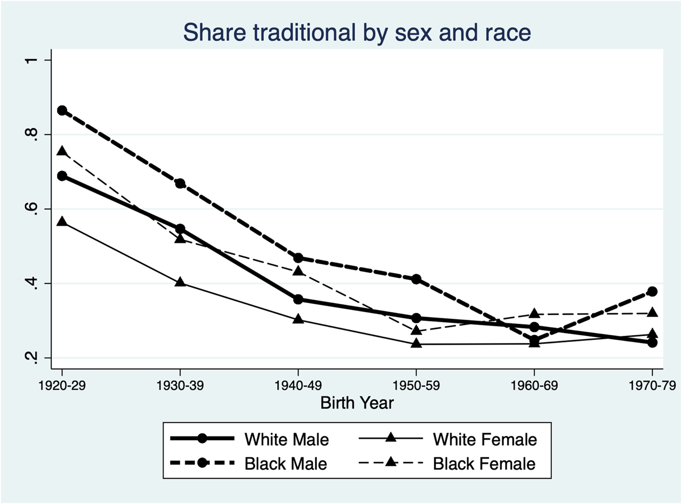
Figure 2. Traditional gender norms by cohort, sex, and race.

Note: Share traditional indicates the share of the marriage-market cohort agreeing with traditional gender norms (“Better for man to work, woman to tend home”), as per the 1977–2014 waves of the General Social Survey. See section 3 for more details.

4. Empirical strategy

The main result from our theoretical model (Implication 1) suggests that gender norm conflict, p _m(1 − p _w), is negatively related to marriage rates. If our model is relevant to the U.S. setting and we empirically control for various factors that can affect marriage rates, other than the gender norm conflict, then we should find a negative correlation between p _m(1 − p _w) and marriage rates. Note that we do not explicitly attempt to identify the causal effect of gender norm conflict on marriage rates, but purely the association between the two which should be consistent with our theoretical model.

Specifically, we estimate the following regression model:

(1)$$\eqalignb{Y_{cm} = & \;\alpha + \pi _1( {{\rm Male}\,{\rm Traditiona}{\rm l}_{cm( r ) }} ) \times ( {{\rm Female}\,{\rm Moder}{\rm n}_{cm( r ) }} ) \cr & + \pi _2( {{\rm Male}\,{\rm Traditiona}{\rm l}_{cm( r ) }} ) + \pi _3( {{\rm Female}\,{\rm Moder}{\rm n}_{cm( r ) }} ) + \delta _c + \gamma _m + \varepsilon _{cm}, \;} $$

where the dependent variable, Y _cm, is the share of respondents that have ever been married belonging to 10-year birth cohort c residing in marriage market m, where the latter is defined by state, race, and skill level.Footnote ¹⁸ An analogous outcome measures the share of respondents who are divorced. Male Traditional_cm(r) is the share of men holding traditional gender norms within cohort c and marriage market, m, which varies geographically at the region level, i.e., m(r).Footnote ¹⁹ Female Modern_cm(r) is the share of women who do not hold traditional gender norms within the same unit of observation, i.e., Female Modern_cm(r) = 1 − Female Traditional_cm(r). All specifications include birth cohort fixed effects, δ _c, market fixed effects, γ _m, i.e., state-race-skill fixed effects.Footnote ²⁰ Finally, ɛ _cm is an error term allowed to be correlated within a state because individuals are assumed to be bounded by their state of residency. Thus, we cluster standard errors at the state level.Footnote ²¹

In our empirical specification, equation (1), we use Male Traditional_cm(r) constructed from our data to approximate p _m, and Female Modern_cm(r) to approximate (1 − p _w). Thus, the product (Male Traditional_cm(r)) × (Female Modern_cm(r)) is our empirical counterpart of gender norm conflict, p _m(1 − p _w). We include both Male Traditional_cm(r) and Female Modern_cm(r) as control variables because if we did not we might falsely attribute either variable's level effect on marriage rates to that of the interaction effect. As described in Appendix 1, including the level effects in our specification also allows us to account for the possibility that our empirical measures of “traditional” men and “modern” women may not necessarily be the same as in the underlying theoretical model. Thus, our approach in bridging the theoretical model and testable empirical specifications is cautious and conservative; however, we note that the main results, as predicted by Implication 1, are qualitatively similar if we do not control for these level effects (Online Appendix Table A2.3). Finally, cohort-level and marriage market-level fixed effects are included throughout to capture other factors, aside from gender norms, that may affect marital outcomes which vary across cohorts and marriage markets, respectively.

Our conceptual framework suggests that π ₁ will be negative when the outcome variable is the ever-married rate and positive when the dependent variable is the divorce rate. Furthermore, we can allow for the possibility that π ₁ may depend on skill level by adding an interaction term between a skilled indicator (college degree) and (Male Traditional_cm(r)) × (Female Modern_cm(r)).Footnote ²² Our framework suggests that the coefficient on this skilled interaction term should carry the same sign as π ₁, indicating an additional marriage market penalty associated with gender norm conflict for skilled individuals.

Note that empirically it is possible for our conflict variable, (Male Traditional_cm(r)) × (Female Modern_cm(r)), to be equally high because men are very traditional and women are moderately modern, men are moderately traditional and women are very modern, or men are moderately traditional and women are moderately modern. Simply exploiting overall variation in the interaction term conceals which relative levels of conflict are driving the results. To address this, we examine heterogeneous effects in marital outcomes across markets based on whether the share of modern women in a market exceeds the share of traditional men.Footnote ²³ Specifically, we estimate the following equation:

(2)$$\eqalignb{Y_{cm} = \, & \alpha + \pi _0( {{\rm Male}\,{\rm Traditiona}{\rm l}_{cm( r ) }} ) \times ( {{\rm Female}\,{\rm Moder}{\rm n}_{cm( r ) }} ) \cr & \times 1( {\rm Female}\,{\rm Moder}{\rm n}_{cm( r ) } > {\rm Male}\,{\rm Traditiona}{\rm l}_{cm( r ) }) \cr & + \pi _1( {{\rm Male}\,{\rm Traditiona}{\rm l}_{cm( r ) }} ) \times ( {{\rm Female}\,{\rm Moder}{\rm n}_{cm( r ) }} ) \cr & + \pi _2( {{\rm Male}\,{\rm Traditiona}{\rm l}_{cm( r ) }} ) + \pi _3( {{\rm Female}\,{\rm Moder}{\rm n}_{cm( r ) }} ) + \delta _c + \gamma _m + \varepsilon _{cm}, \;} $$

where 1(Female Modern_cm(r) > Male Traditional_cm(r)) is an indicator variable capturing whether the share of modern women exceeds the share of traditional men. The coefficient of interest, π ₀, captures the additional change in marital outcomes stemming from conflict in markets in which women are more modern than men are traditional relative to the impact of gender norm conflict in markets in which men are more traditional than women are modern or in which men and women are similarly traditional. Thus, we interpret π ₀ as the impact of gender norm conflict driven by markets in which women are especially modern.

In further extensions, we explore heterogeneous impacts for different racial groups by estimating equation (1) separately for Black and white marriage markets. We also investigate the relationship between gender norm conflict and the presence of children, our proxy for marriage quality and marital investments.

5. Results

5.1 Main results

Table 2 presents the main results linking gender norm conflict with marriage and divorce. Consistent with our conceptual framework and theoretical prediction (Implication 1), marriage rates for both men and women are statistically significantly lower in markets with greater conflict over gender norms. This is clear from the negative coefficients on the interaction term in columns 1 and 2 (point estimates of −0.353 and −0.426, respectively). To interpret the magnitudes of these effects, we consider the impact of an increase in gender norm conflict, as measured by the interaction term (mean = 0.25, standard deviation = 0.06), on each of the dependent variables. This exercise suggests that a one standard deviation increase in gender norm conflict is associated with a decrease in marriage rates of about 2.4% for men (−0.353 × 0.06/0.87) and 2.9% for women (−0.426 × 0.06/0.89), relative to the average marriage rates of each group (87% for men and 89% for women). While we do not place theoretical emphasis on the magnitudes of the other coefficients in the regression model, from an empirical perspective, it is also interesting to note that the share of traditional men is strongly positively correlated with marriage (point estimates 0.345 and 0.393 for men and women, respectively), while the share of modern women in the market is statistically insignificant and close to zero in the same specification (columns 1 and 2). Also noteworthy is the fact that the R ² is high for these specifications, in part due to the fact that our marriage market fixed effects are able to explain a large portion of the variation in marital outcomes.

Table 2. Gender norm conflict and marital outcomes

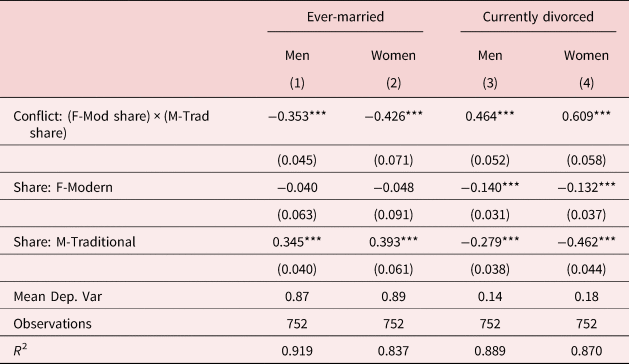
Note: The unit of observation is a cell defined by birth cohort and marriage market, where the latter is defined by race, skill, and state. Dependent variables measure marriage and divorce rates from ACS samples using population weights. M-Traditional measures share of men agreeing with traditional gender norms (“Better for man to work, woman to tend home”) within a cell defined by race-sex-skill-region based on GSS samples. F-Modern measures 1-share of women agreeing with traditional gender norms. Conflict: (F-Mod share) × (M-Trad share) measures interaction between F-Modern and M-Traditional shares. All models include cohort fixed effects as well as fixed effects for the marriage market which varies by race, skill, and state. See further sample details in section 3 of the main text.

Robust standard errors, clustered at state level, reported in parentheses.

***p < 0.01, **p < 0.05, *p < 0.1.

At the same time, the remaining columns of Table 2 show that for both men and women, all else equal, divorce rates are higher in marriage markets with greater conflict over gender norms (point estimates 0.464 and 0.609, respectively), as expected from the discussion above. Interpreting the magnitudes of these coefficients indicates that a one standard deviation increase in gender norm conflict is associated with a higher divorce rate of about 20% for both men and women, relative to the average rates of divorce for each group (14% for men and 18% for women). These estimates are statistically significant at the 1% level, and the magnitudes individually outweigh the negative coefficients on the shares of modern women and traditional men in the market.Footnote ²⁴

One concern with these results is that they may be driven by unobserved correlations between gender norms and differences in labor market outcomes for men and women. To address this, Table 3 controls for the gender difference in employment rates within each marriage market.Footnote ²⁵ The resulting estimates might be interpreted to control for relative labor market opportunities for men and women which should affect the value of marriage; however, caution is warranted since gender norms are likely to be correlated with labor supply and hence complicate the estimate of a causal effect absent exogenous variation in gender-specific labor demand [Autor et al. (Reference Autor, Dorn and Hanson2019)]. Thus, the lack of statistically significant estimates on the added control variable may simply suggest that labor market outcomes are bound up with gender norms in such a way that gender differences in employment rates have little impact on marital outcomes after accounting for views on the role of men and women in the labor market. At the same time, the fact that the point estimates on gender norm conflict are virtually unchanged after controlling for this variation suggests that the observed correlation between gender norm conflict and marriage rates is not driven solely by gender gaps in labor market outcomes.

Table 3. Gender norm conflict and marital outcomes, controlling for gender difference in employment rate

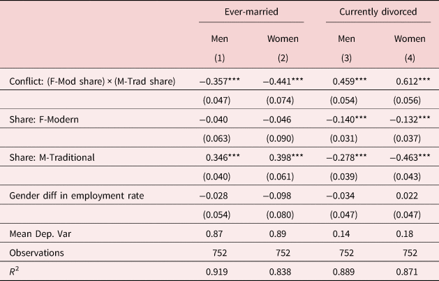
Note: The unit of observation is a cell defined by birth cohort and marriage market, where the latter is defined by race, skill, and state. Dependent variables measure marriage and divorce rates from ACS samples using population weights. M-Traditional measures share of men agreeing with traditional gender norms (“Better for man to work, woman to tend home”) within a cell defined by race-sex-skill-region based on GSS samples. F-Modern measures 1-share of women agreeing with traditional gender norms. Conflict: (F-Mod share) × (M-Trad share) measures interaction between F-Modern and M-Traditional shares. The gender difference in employment rates is calculated as mean male employment rate−mean female employment rate within each marriage market, where the employment rate is calculated for individuals who report being in the labor force. All models include cohort fixed effects as well as fixed effects for the marriage market which varies by race, skill, and state. See further sample details in section 3 of the main text.

Robust standard errors, clustered at state level, reported in parentheses.

***p < 0.01, **p < 0.05, *p < 0.1.

5.2 Extensions

Our first main extension allows for the possibility that gender norm conflict may have differential impacts on marital outcomes depending on people's labor market opportunities. Specifically, Table 4 explores heterogeneous effects by skill. For women, we see that in addition to the negative impact of gender norm conflict on marriage rates (point estimate −0.244), we also observe an additional negative impact for skilled groups in particular (point estimate −0.184), and both estimates are statistically significant at the 5% level. As predicted, these estimates suggest an additional negative impact of gender norm conflict for women in skilled markets, although the overall impacts of gender norm conflict on marriage rates are still small relative to average rates of marriage. The coefficient measuring differential impacts of gender norm conflict for skilled men is slightly smaller in magnitude and statistically significant at the 10% level (point estimate −0.116 in column 1).

Table 4. Gender norm conflict and marital outcomes by skill level

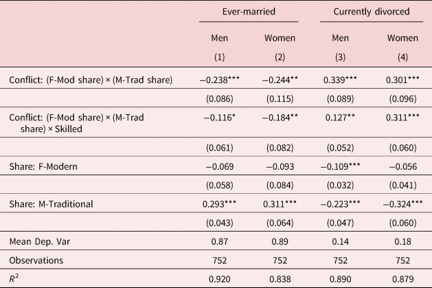
Note: The unit of observation is a cell defined by birth cohort and marriage market, where the latter is defined by race, skill, and state. Dependent variables measure marriage and divorce rates from ACS samples using population weights. M-Traditional measures share of men agreeing with traditional gender norms (“Better for man to work, woman to tend home”) within a cell defined by race-sex-skill-region based on GSS samples. F-Modern measures 1-share of women agreeing with traditional gender norms. Conflict: (F-Mod share) × (M-Trad share) measures interaction between F-Modern and M-Traditional shares. Conflict: (F-Mod share) × (M-Trad share) × Skilled further interacts the conflict–product interaction term with whether individuals in the market have a college degree. All models include cohort fixed effects as well as fixed effects for the marriage market which varies by race, skill, and state. See further sample details in section 3 of the main text.

Robust standard errors, clustered at state level, reported in parentheses.

***p < 0.01, **p < 0.05, *p < 0.1.

At the same time, we observe heterogeneous effects by skill on divorce rates for both men and women (columns 3 and 4). In particular, the coefficients on the interaction term between gender norm conflict and the skilled indicator are positive and statistically significant at the 5% and 1% levels for men and women (point estimates 0.127 and 0.311), respectively. Note that the coefficient estimates on the gender norm conflict measure alone are also positive and statistically significant at the 1% level (0.339 and 0.301 for men and women, respectively). Thus, both skilled and unskilled groups face a higher likelihood of divorce due to gender norm conflict, but skilled individuals face a statistically significantly higher likelihood of divorce when there is a greater degree of gender norm conflict, relative to their unskilled counterparts. For women, we note that the coefficient on the interaction term between gender norm conflict and skill is very close in magnitude to the coefficient on the gender norm conflict term alone, suggesting that skilled women face an especially large penalty associated with gender norm conflict in the marriage market.Footnote ²⁶ This is consistent with the hypothesis that gender norm conflict especially impacts marital happiness and agreement over the longer run for individuals that are relatively skilled and who likely face better economic opportunities outside of marriage.

As noted above, our conflict variable is silent on how different types of conflict affect marital outcomes. Table 5 explores whether the impacts of gender norm conflict are higher when conflict is primarily driven by the share of modern women exceeding the share of traditional men. While we see no statistically significant impact of the interaction term of interest on marriage rates, we again see a greater likelihood of divorce associated with markets in which the share of modern women is higher than the share of traditional men (coefficient estimates of 0.058 for men and 0.056 for women). This suggests that there is an additional marriage market penalty of gender norm conflict if the market is one in which women are especially modern.

Table 5. Heterogeneity in gender norm conflict

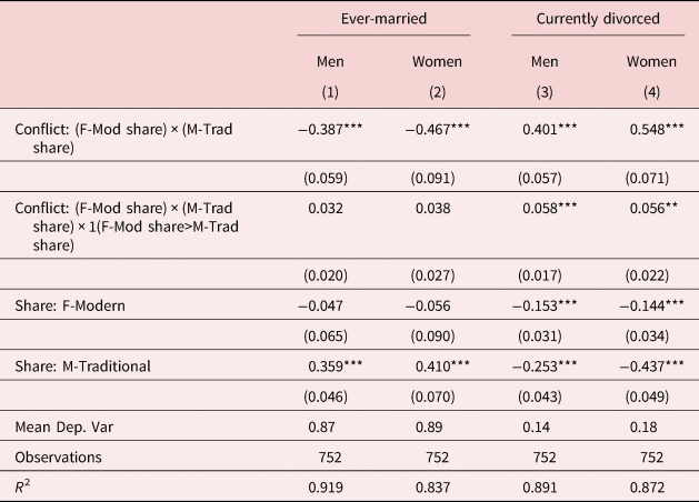
Note: The unit of observation is a cell defined by birth cohort and marriage market, where the latter is defined by race, skill, and state. Dependent variables measure marriage and divorce rates from ACS samples using population weights. M-Traditional measures share of men agreeing with traditional gender norms (“Better for man to work, woman to tend home”) within a cell defined by race-sex-skill-region based on GSS samples. F-Modern measures 1-share of women agreeing with traditional gender norms. Conflict: (F-Mod share) × (M-Trad share) measures interaction between F-Modern and M-Traditional shares. Conflict: (F-Mod share) × (M-Trad share) × 1(F-Mod share>M-Trad share) further interacts the conflict–product interaction term with an indicator for whether the share of modern women in the market exceeds the share of traditional men. All models include cohort fixed effects as well as fixed effects for the marriage market which varies by race, skill, and state. See further sample details in section 3 of the main text.

Robust standard errors, clustered at state level, reported in parentheses.

***p < 0.01, **p < 0.05, *p < 0.1.

We extend the analysis by dividing the sample by race to explore whether there are differential effects for Black and white groups. Online Appendix Table A2.4 presents the results from estimating equation (1) for marriage markets by racial group. Results show a statistically significant negative relationship between gender norm conflict and marriage rates (Panel A) that is driven mainly by white groups; however, the magnitude is smaller than the results from the pooled sample (coefficient estimate of −0.123 for white men and −0.098 for white women vs. −0.353 for all men and −0.426 for all women from Table 2). Results for divorce rates (Panel B) are closer in magnitude to estimates from above, and again show greater statistical significance for white groups (coefficient estimate of 0.563 for white men and 0.626 for white women vs. 0.464 for all men and 0.609 for all women from Table 2). Together, these results suggest that the results from above are driven by white groups; however, the statistically insignificant results for Black groups may be due to the much smaller sample size (155 Black market-cohort observations vs. 597 white market-cohort observations). The relative strength of results across racial groups may also be due to higher variance in the estimates of gender norm conflict drawn for Black marriage markets from the GSS, which typically have a much smaller sample size than for analogous white marriage markets.

Finally, Online Appendix Table A2.5 provides suggestive evidence of the impact of gender norm conflict on marriage quality and marital investments, as proxied by whether children are present in the household. Importantly, we note that these results should be interpreted with caution, as one caveat of the outcome variable is that data availability limits us to examining whether children reside in the household at the time of the survey, as opposed to whether the specific marital union has produced any children.Footnote ²⁷ Nevertheless, we see that the coefficient of interest is negative and statistically significant at the 1% level for both men and women, suggesting that children are less likely to be present if there is greater gender norm conflict in the marriage market.Footnote ²⁸ For women, the magnitude of the coefficient suggests that a one standard deviation increase in gender norm conflict is associated with a decline in the share of men with children in the household of about 20% (−1.053 × 0.06/0.31), while the same change would result in a decline in the share of women with children in the household of about 9% (−0.580 × 0.06/0.37), relative to the average shares of each group with children in the household (31% for men and 37% for women). Data caveats notwithstanding, this correlation is consistent with a model in which gender norm conflict decreases marriage quality, resulting in a decline in fertility.

6. Conclusion

The evidence from our empirical analysis of the link between gender norm conflict and marital outcomes has confirmed our theoretical model predictions: greater dissimilarity between men's and women's views on their roles within marriage is associated with lower marriage rates and higher divorce rates. Specifically, our main results suggest that a one standard deviation increase in gender norm conflict is associated with a drop in marriage rates of about 2.4% for men and 2.9% for women. The same change is associated with an increase of about 20% in divorce rates for both men and women. Moreover, heterogeneity analysis indicates gender norm conflict has even greater impacts in skilled marriage markets where it is associated with even lower marriage rates and higher divorce rates, suggesting greater marriage market penalties associated with gender norm conflict for skilled men and women. In extensions, we find that these results are mainly driven by white marriage markets, as well as evidence that the impact of gender norm conflict is higher when the share of modern women exceeds the share of traditional men. Finally, we find suggestive evidence that increases in gender norm conflict arising from increases in the share of modern women are associated with a lower likelihood of children present in the home, which would be consistent with a model in which greater gender norm conflict led to lower marriage quality and lower marital investments. Overall, these results are consistent with our conceptual framework linking marital outcomes with gender norms, the division of labor within marriage, and labor market opportunities outside the marital household.

While these findings represent a significant step forward in understanding how gender norms relate to economic outcomes, one important limitation of this work is that we have followed the literature in taking gender norms as exogenously given. Further research should identify exogenous sources of variation in gender norms and ideally explore the determinants of gender norms themselves, in order to better understand their wider impacts.

Supplementary material

The supplementary material for this article can be found at https://doi.org/10.1017/dem.2021.7.

Acknowledgement

We thank participants at the Society of Economics of the Household inaugural meeting and the Western Economic Association International conference. Lee acknowledges the support of the New Faculty Startup Fund from Seoul National University.

Appendix 1: The link between theoretical components and the empirical specification

Suppose that we explain the marriage rate in cohort c, marriage market m(r), with the gender norm conflict measure (p _{m, cm(r)}) × (1 − p _{w, cm(r)}), cohort fixed effects (δ _c), marriage market fixed effects (γ _m), and random shocks (ɛ_cm). The latter three variables are included to capture the factors other than gender norm conflict that can influence marriage rates. Note that p _{m, cm(r)} refers to the share of men holding traditional gender norms in cohort c, marriage market m(r), while 1 − p _{w, cm(r)} is the share of women holding modern gender norms in cohort c, marriage market m(r). The empirical model would then be:

(*)$$Y_{cm} = \theta + \pi ( {\,p_{m, \;cm( r ) }} ) \times ( {1-p_{w, \;cm( r ) }} ) + \delta _c{\rm \;} + \gamma _m + \varepsilon _{cm}$$

The key coefficient of interest is π, which is predicted to be negative (Implication 1).

To estimate the equation (*), we construct two variables from the General Social Survey (GSS) to approximate our theoretical measures of the share of men holding traditional gender norms and share of women holding modern gender norms in cohort c, marriage market m(r), i.e., p _{m, cm(r)} and (1 − p _{w, cm(r)}), respectively. However, there is no guarantee that the two variables we construct from the data are exactly the same as p _{m, cm(r)} and (1 − p _{w, cm(r)}). Rather, more realistically, the two variables from the GSS are expected to be correlated with their theoretical counterparts. Suppose that

$$p_{m, \;cm( r ) } = c_1{\rm Male}\,{\rm Traditiona}{\rm l}_{cm( r ) } + \mu _1, \;$$

$$( {1-p_{w, \;cm( r ) }} ) = c_2{\rm Female}\,{\rm Moder}{\rm n}_{cm( r ) } + \mu _2, \;$$

where Male Traditional_cm(r) is the actual share of men with traditional gender norms from the GSS in cohort c, marriage market m(r), while p _{m, cm(r)} is the theoretical measure of the share of men holding traditional gender norms in that cohort and marriage market. c ₁ is a positive number and μ ₁ is a constant. Similarly, Female Modern_cm(r) is the actual share of women with modern gender norms from our data while 1 − p _{w, cm(r)} is the theoretical counterpart. c ₂ is a positive number and μ ₂ is a constant.

By replacing p _{m, cm(r)} and 1 − p _{w, cm(r)} with Male Traditional_cm(r) and Female Modern_cm(r), the (*) equation turns into

$$\eqalign{Y_{cm} = & \;\theta + \pi \mu _1\mu _2 + \pi c_1c_2\,{\rm Male}\,{\rm Traditiona}{\rm l}_{cm( r ) }\,{\rm Female}\,{\rm Moder}{\rm n}_{cm( r ) } \cr & + \pi c_1\mu _2\,{\rm Male}\,{\rm Traditiona}{\rm l}_{cm( r ) } + \pi c_2\mu _1\,{\rm Female}\,{\rm Moder}{\rm n}_{cm( r ) } + \delta _c + \gamma _m + \varepsilon _{cm}.} $$

Let α = θ + πμ ₁μ ₂, π ₁ = πc ₁c ₂, π ₂ = πc ₁μ ₂, and π ₃ = πc ₂μ ₁. Then, we have the following equation to estimate:

$$\eqalign{Y_{cm} = & \;\alpha + \pi _1\,{\rm Male}\,{\rm Traditiona}{\rm l}_{cm( r ) }\,{\rm Female}\,{\rm Moder}{\rm n}_{cm( r ) } \cr & + \pi _2\,{\rm Male}\,{\rm Traditiona}{\rm l}_{cm( r ) }{\rm \;} + \pi _3\,{\rm Female}\,{\rm Moder}{\rm n}_{cm( r ) } + \delta _c + \gamma _m + \varepsilon _{cm}, \;} $$

which is reported as equation (1) in the manuscript.

If our variables Male Traditional_cm(r), Female Modern_cm(r) are accurate measures of their theoretical counterparts (i.e., c ₁ = c ₂ = 1, μ ₁ = μ ₂ = 0), then our estimation results will yield π ₂ and π ₃ to be zero, and not affect our estimate of π ₁. Note also that as long as our variables are positively correlated with their theoretical counterparts (i.e., c ₁ > 0 and c ₂ > 0), the sign of π ₁ should be estimated to be the same as that of π. As we show in the paper, our model prediction (π < 0) is in fact consistent with the empirics (estimate of π ₁ < 0): the sign of the conflict term is negative in Table 2, as predicted in Implication 1.

Furthermore, if in fact Male Traditional_cm(r) is the same as p _{m, cm(r)} and Female Modern_cm(r) is the same as (1 − p _{w, cm(r)}), then adding irrelevant control variables in our regression (equation (1)) should not bias our results. If this were the case, we would also expect the estimated coefficients of Male Traditional_cm(r) and Female Modern_cm(r) to be statistically no different from zero. Nevertheless, for reference, the results of estimating equation (*) are provided in Online Appendix Table A2.3 which also indicates a negative correlation between gender norm conflict and marriage rates, as predicted in Implication 1.

Footnotes

¹ These differences across sexes may simply arise due to relative receptiveness of the transmission of gender norms between men and women in different contexts, but we do not take a stand on that process or those determinants, and instead follow the literature in taking gender norms themselves as exogenously given.

² An alternative model specification might link a higher net benefit of marriage (individual utility from marriage relative to remaining single) for individuals with the same gender norm (i.e., who have less gender norm conflict within the marriage) more directly with benefits stemming from spouses sharing similar views on the role of men and women within marriage. For example, marriages between two traditional spouses may benefit from complete specialization aligned with the traditional gender norm (i.e., where the man works and the woman tends to the home). At the same time, marriages between two modern spouses may benefit from being able to insure each other against shocks due to both spouses' participation in the labor market. Finally, the net benefit of marriage could also be higher for partners matched on gender norms if the latter were correlated with other tastes such that the husband and wife had similar preferences for the household public good. We abstract from these explicit characterizations in this simple model.

³ For simplicity, we use the standard normal distribution to illustrate the model implications. The results hold under a broader class of distributions. Likewise, the i.i.d. assumption on the random shocks for men and women can be relaxed as well.

⁴ Our model ignores the possibility that people may get utility from having a child or children. This simplification is easily addressed as long as the number of children is exogenously given. Note that Bertrand et al. (Reference Bertrand, Cortes, Olivetti and Pan2018) also assume an exogenous number of children for a married couple.

⁵ Our assumption that α _m for traditional men is zero implies that the marriage benefit to them is only through household production, not through sharing public goods such as TV and housing. Although this assumption is extreme, mainly introduced to simplify the analysis, we can view this assumption as depicting the situation in which the disutility of having a working wife offsets the benefit from public goods partly provided by her income.

⁶ Note that a strict ranking of the likelihood of marriage across all male–female matches is not possible given the model's limited assumptions. Also note that the model does not predict assortative mating along gender norms as there are no complementarities between men and women's gender norms to produce a result in the style of Lam (Reference Lam1988). Instead, the central theoretical prediction stemming from the model is that the likelihood of marriage should be lowest between the traditional man and modern woman.

⁷ Specifically, suppose that the value of marriage in time t is the sum of the value of marriage measured at the time of marriage and random shocks realized in time t:

$$V_{m, t} = V_m( {w_m, \;\;w_w, \;q_m} ) + \omega _{m, t}\,{\rm and}\,V_{w, t} = V_w( {w_m, \;\;w_w, \;q_m} ) + \omega _{w, t}, \;$$

where

$$E( {\omega_{m, t}{\rm \vert }w_m, \;\;w_w, \;q_m} ) = E( {\omega_{w, t}{\rm \vert }w_m, \;\;w_w, \;q_w} ) = 0.$$

For simplicity, we assume that a person's value of remaining single is unchanged over time. Then, man m will remain married to woman w as long as $q_m + \omega _{m, t} \ge q_m^\ast$ and woman w will remain married if $q_w + \omega _{w, t} \ge q_w^\ast$. As shown above, if man m has traditional gender norms and woman w has modern gender norms, their threshold reservation match qualities, $q_m^\ast$ and $q_w^\ast$, are higher than those of their counterparts. Thus, even if they agreed to marry because of unusually high q _m and q _w, they are more likely to violate at least one of the two inequality conditions once they are exposed to negative random shocks (ω _m,t or ω _w,t).

⁸ For example, Hitsch et al. (Reference Hitsch, Hortaçsu and Ariely2010) document that in the United States, people exhibit strong same-race preferences in online dating and Furtado (Reference Furtado2012) documents high rates of ethnic endogamy.

⁹ Stevenson (Reference Stevenson2007) shows that when the risk of divorce increases due to the adoption of unilateral divorce laws across the United States, marriage-specific investments fall, including the likelihood of having children.

¹⁰ While there are 30 waves of GSS available over this range of years, only 19 of those surveys include the gender norm question used in our analysis. We merge all these waves together to construct our gender norm variables at the market level.

¹¹ This definition follows in the spirit of Bertrand et al. (Reference Bertrand, Cortes, Olivetti and Pan2015) and Bertrand et al. (Reference Bertrand, Cortes, Olivetti and Pan2018). We also follow their lead in aggregating to the state level; however, our main results regarding the relationship between gender norm conflict, marriage, and divorce rates are robust to individual-level analysis. This makes sense as all of the individual-level results from the theoretical model should aggregate. For brevity, we sometimes refer to our units of observation, i.e., the marriage market-cohorts, simply as “markets.”

¹² Bertrand et al. (Reference Bertrand, Cortes, Olivetti and Pan2015) discuss the empirical evidence for the patterns of homophily which support grouping individuals into marriage markets in this style. While individuals are assigned to their state of residency, the results are robust to controlling for the share of individuals currently residing in their state of birth by race-skill-state-cohort-sex groupings. This should assuage any concerns that our results may be driven by selective migration.

¹³ We collapse the regional GSS identifier to indicate Northeast, Midwest, South, and West to preserve sample size.

¹⁴ We define the unit of observation at the state, rather than region, level to ensure that our model incorporates important variation in marriage markets at the state level that would otherwise be lost. Moreover, we expect that the coarser level of variation in the explanatory variable of interest, relative to the outcome variable, will make it harder to find statistically significant relationships. Thus, our empirical strategy can be regarded as relatively conservative compared with one that allowed for state-level variation in gender norms.

¹⁵ Limiting the sample to individuals who are at least 30 years old ensures that our analysis excludes young adults who are less likely to be active participants in marriage markets and addresses concerns regarding the rise in age at first marriage across cohorts. This threshold is close to the current median age at first marriage for men (30.5) and women (28.1) in the United States [U.S. Census Bureau (2020)]. Though our data come from two sources, a comparison of average demographic variables across ACS and GSS samples with these thresholds suggests that the two data sources are sampling similar populations. While our main results are similar if we impose no threshold on the number of individuals per market-cohort observation, intuitively, it makes sense that including some threshold is needed to ensure that the averages are reasonably representative of individuals in a market-cohort. More formally, econometric studies of pseudo-panels following Deaton (Reference Deaton1985) conclude that repeated cross-sections can be used to infer cohort-level behavior provided the samples are sufficiently large and suggest a practical benchmark of 100 individuals per cohort [Verbeek and Nijman (Reference Verbeek and Nijman1992)]. Our main results regarding the relationship between marriage and divorce rates and gender norm conflict are robust to raising the number of individuals within each market-cohort to 100 overall (50 men and 50 women); however, the number of market-cohort observations drops considerably with this restriction, in particular for non-white marriage markets, thus limiting the extent to which we can engage in further heterogeneity analysis.

¹⁶ The share of currently divorced individuals is calculated as the number of currently divorced individuals divided by the number of individuals whose marital status indicates they have ever been married. We are not able to observe whether individuals have ever been divorced, and say, remarry.

¹⁷ Examining descriptive statistics across marriage markets suggests that markets with the highest levels of conflict (greater than the 75^th percentile level of conflict level, i.e., 0.285) are more likely to be white, from the South, consist of older cohorts, and have no college degrees (Online Appendix Table A2.2).

¹⁸ Note that this measure captures all marriages of individuals in each market-cohort and does not specify to whom those individuals are married. While Bertrand et al. (Reference Bertrand, Cortes, Olivetti and Pan2015) show that cross-market marriages are rare, further investigation of the link between cross-market marriages and gender norms would be an interesting extension of this work.

¹⁹ As discussed in section 3, the gender norm variables vary at the cohort-market region level due to data limitations in GSS public data sources, reflected in the subscript m(r).

²⁰ This specification follows other papers in the literature [Bertrand et al. (Reference Bertrand, Cortes, Olivetti and Pan2015)], and reflects an empirical model that is consistent with modeling the observations as a marriage market pseudo-panel. As such, controlling for characteristics of the marriage market that do not vary over time (i.e., across cohorts) is important; however, our main results are also robust to including separate fixed effects for state, race, and skill level.

²¹ We follow the literature in clustering at the state level [Bertrand et al. (Reference Bertrand, Cortes, Olivetti and Pan2015), Bertrand et al. (Reference Bertrand, Cortes, Olivetti and Pan2018)], which we also view as conservative in that it allows for the possibility that individuals may find their spouses outside their specific marriage markets within a state, which might in turn generate spillover effects. Clustering at the state level thus allows for random shocks to be correlated across different marriage markets within the same state. However, some may view treatment assignment as the appropriate clustering unit as per Abadie et al. (Reference Abadie, Athey, Imbens and Wooldridge2017) and thus prefer clustering at the level of variation of our independent variable of interest, i.e., the region-race-cohort-skill level. Our main results are robust to clustering at that level as well as clustering at the region level with wild-bootstrap techniques implemented using Webb weights and 1,000 replications, due to the small number of regions.

²² Alternatively, we can include (Male Traditional_cm(r)) × Skilled_cm as well as (Female Traditional_cm(r)) × Skilled_cm in equation (1). Our main results are robust to controlling for those interaction terms, though we lose statistical significance in the ever-married regression for men.

²³ Approximately 78% of the markets in our sample have a higher share of modern women than traditional men.

²⁴ One might expect that couples who select into marriage despite gender norm conflict may have relatively high match quality. While we cannot control for match quality directly, these results suggest that on average the impact of conflict over gender norms on divorce ultimately outweighs any positive selection into marriage.

²⁵ Specifically, the gender difference in employment rates is calculated as the mean employment rate for men minus the mean employment rate for women within each marriage market, where the employment rate is calculated for individuals who report being in the labor force.

²⁶ The literature on family economics has highlighted the potential trade-offs in human capital investment for women due to the presence of both marriage market returns and labor market returns to education [Chiappori et al. (Reference Chiappori, Iyigun and Weiss2009), LaFortune (Reference LaFortune2013)]. On the one hand, human capital investment increases women's labor market opportunities, while on the other hand, the investment could lead to worse marriage market outcomes for women due to the presence of traditional gender norms. Our results are consistent with this broad line of research suggesting a marriage market penalty for skilled women [e.g., Bertrand et al. (Reference Bertrand, Cortes, Olivetti and Pan2018)].

²⁷ This limitation may be especially problematic for the oldest individuals in our sample, for whom the presence of adult children in the home may be more likely to indicate reverse transfers from children to parents. While it is not clear how this might bias the results, some may be concerned that these living arrangements may be correlated with traditional values. To address this, we have tried dropping the two oldest birth cohorts from the sample (birth years 1920–1939) and find qualitatively similar results to those discussed here.

²⁸ This is similar to the result from Stevenson (Reference Stevenson2007) showing that an increase in the risk of divorce introduced by the adoption of unilateral divorce laws decreases the likelihood of having children.

References

Abadie, Alberto, Athey, Susan, Imbens, Guido W. and Wooldridge, Jeffrey (2017) When Should You Adjust Standard Errors for Clustering? NBER Working Paper No. 24003.Google Scholar

Akerlof, George A. and Kranton, Rachel E. (2000) Economics and identity. Quarterly Journal of Economics 115(3), 715–753.CrossRef Google Scholar

Alesina, Alberto, Giuliano, Paola and Nunn, Nathan (2013) On the origins of gender roles: women and the plough. Quarterly Journal of Economics 128(2), 469–530.CrossRef Google Scholar

Autor, David, Dorn, David and Hanson, Gordon (2019) When work disappears: manufacturing decline and the falling marriage market value of young men. American Economic Review: Insights 1(2), 161–178.Google Scholar

Becker, Gary S. (1973) A theory of marriage: part I. Journal of Political Economy 81(4), 813–846.CrossRef Google Scholar

Bertrand, Marianne, Cortes, Patricia, Olivetti, Claudia and Pan, Jessica (2016) Social Norms, Labor Market Opportunities, and the Marriage Gap for Skilled Women. NBER Working Paper No. 22015.CrossRef Google Scholar

Bertrand, Marianne, Cortes, Patricia, Olivetti, Claudia and Pan, Jessica (2018) Social Norms, Labor Market Opportunities, and the Marriage Gap for Skilled Women. IZA DP No. 11382.Google Scholar

Bertrand, Marianne, Kamenica, Emir and Pan, Jessica (2015) Gender identity and relative income within households. Quarterly Journal of Economics 130(2), 571–614.CrossRef Google Scholar

Chiappori, Pierre-Andre, Iyigun, Murat and Weiss, Yoram (2009) Investment in schooling and the labor market. American Economic Review 99(5), 1689–1713.10.1257/aer.99.5.1689CrossRef Google Scholar

Choo, Eugene and Siow, Aloysius (2006) Who marries whom and why. Journal of Political Economy 114(1), 175–201.CrossRef Google Scholar

Deaton, Angus (1985) Panel data from time series of cross sections. Journal of Econometrics 30, 109–126.CrossRef Google Scholar

Farré, Lídia and Vella, Francis (2012) The intergenerational transmission of gender role attitudes and its implications for female labour force participation. Economica 80(318), 219–247.CrossRef Google Scholar

Fernandez, Raquel, Fogli, Alessandra and Olivetti, Claudia (2004) Mothers and sons: preference formation and female labor force dynamics. Quarterly Journal of Economics 119(4), 1249–1299.CrossRef Google Scholar

Furtado, Delia (2012) Human capital and interethnic marriage decisions. Economic Inquiry 50(1), 82–93.CrossRef Google Scholar PubMed

Giménez-Nadal, J. Ignacio, Mangiavacchi, Lucia and Piccoli, Luca (2019) Keeping inequality at home: the genesis of gender roles in housework. Labour Economics 58, 52–68.CrossRef Google Scholar

Giménez-Nadal, J. Ignacio, Molina, Jose and Sevilla-Sanz, Almudena (2012) Social norms, partnerships and children. Review of Economics of the Household 10(2), 215–236.CrossRef Google Scholar

Hitsch, Günter J., Hortaçsu, Ali and Ariely, Dan (2010) What makes you click? Mate preferences and matching outcomes in online dating. Quantitative Marketing and Economics 8(4), 393–427.CrossRef Google Scholar

Kawaguchi, Daiji and Lee, Soohyung (2016) Brides for sale: cross-border marriages and female immigration. Economic Inquiry 55(2), 1–22.Google Scholar

LaFortune, Jeanne (2013) Making yourself attractive: pre-marital investments and the returns to education in the marriage market. American Economic Journal: Applied Economics 5(2), 151–178.Google Scholar

Lam, David (1988) Marriage markets and assortative mating with household public goods: theoretical results and empirical implications. Journal of Human Resources 23(4), 462–487.CrossRef Google Scholar

Ruggles, Steven, Flood, Sarah, Goeken, Ronald, Grover, Josiah, Meyer, Erin, Pacas, Jose and Sobek, Matthew (2019) IPUMS USA: Version 9.0 [dataset]. Minneapolis, MN: IPUMS. https://doi.org/10.18128/D010.V9.0.CrossRef Google Scholar

Sevilla-Sanz, Almudena (2010) Household division of labor and cross-country differences in household formation rates. Journal of Population Economics 23(1), 225–249.CrossRef Google Scholar

Smith, Lones (2006) The marriage model with search frictions. Journal of Political Economy 114(6), 1124–1144.CrossRef Google Scholar

Smith, Tom W., Davern, Michael, Freese, Jeremy and Hout, Michael (2018) General Social Surveys, 1977–2014. Sponsored by National Science Foundation. Chicago, IL: NORC at the University of Chicago and Storrs, CT: The Roper Center for Public Opinion Research, University of Connecticut.Google Scholar

Stevenson, Betsey (2007) The impact of divorce laws on marriage-specific capital. Journal of Labor Economics 25(1), 75–94.CrossRef Google Scholar

U.S. Census Bureau (2020) Historical Marital Status Tables. Available at https://www.census.gov/data/tables/time-series/demo/families/marital.html.Google Scholar

Verbeek, M. and Nijman, T. (1992) Can cohort data be treated as genuine panel data? Empirical Economics 17, 9–23.CrossRef Google Scholar

Table 1. Gender norms and probability of marriage for men and women

Figure 1. Marriage rates by cohort, sex, and race.Note: Share married indicates the share of the marriage-market cohort that has ever been married, as per the 2002, 2006, 2010, and 2014 waves of the American Community Survey. See section 3 for more details.

Figure 2. Traditional gender norms by cohort, sex, and race.Note: Share traditional indicates the share of the marriage-market cohort agreeing with traditional gender norms (“Better for man to work, woman to tend home”), as per the 1977–2014 waves of the General Social Survey. See section 3 for more details.

Table 2. Gender norm conflict and marital outcomes

Table 3. Gender norm conflict and marital outcomes, controlling for gender difference in employment rate

Table 4. Gender norm conflict and marital outcomes by skill level

Table 5. Heterogeneity in gender norm conflict

Antman et al. supplementary material

Antman et al. supplementary material 1

File 29.4 KB

Antman et al. supplementary material

Antman et al. supplementary material 2

File 34 KB

Article contents

Gender norm conflict and marital outcomes

Abstract

Keywords

JEL classification

1. Introduction

2. Conceptual framework

2.1 Background and intuition

2.2 Setup

2.2.1 Value of marriage

2.2.2 Value of singlehood

2.3 Marriage market

2.4 Theoretical implications

2.4.1 Main results

2.4.2 Extensions

3. Data and descriptive statistics

4. Empirical strategy

5. Results

5.1 Main results

5.2 Extensions

6. Conclusion

Supplementary material

Acknowledgement

Appendix 1: The link between theoretical components and the empirical specification

Footnotes

References

Antman et al. supplementary material

Antman et al. supplementary material

Save article to Kindle

Save article to Dropbox

Save article to Google Drive

Reply to: Submit a response

Your details

You have entered the maximum number of contributors

Conflicting interests