1. INTRODUCTION
During the last 60 years, dramatic changes have taken place in the United States in the hours allocated to market production as a function of sex and marital status. The most striking change is the almost threefold increase in the hours worked by married women. This change has occurred over a period during which married men’s hours have declined slightly and those of single individuals, both women and men, have been virtually unchanged (see Figure 1A). Our objective in this paper is to study the validity of three alternative hypotheses for why these changes have occurred: (i) the changes are a result of improvements in the technology for producing home goods, (ii) they follow from overall income growth if home goods are inferior, and (iii) they are a result of a reduction in the gender wage gap.

Figure 1. U.S. hours and wage ratios since 1950. A. Market hours of work per week. B. Ratio of women’s to men’s wage rates (%).
To this end, we construct a dynamic general equilibrium model of the macroeconomy that differs only minimally from standard models with home production and savings [see Benhabib, Rogerson and Wright (Reference Benhabib, Rogerson and Wright1991) and McGrattan, Rogerson and Wright (Reference McGrattan, Rogerson and Wright1997)]. These changes include the explicit distinction between single (both female and male) and married households (and the women and men in such a household) and specific decisions about human capital accumulation. All agents care about both home and market goods as well as the leisure of the parties in the household. We assume that both home and market goods require quality adjusted labor (time augmented with human capital) to be produced. These agents interact, as price takers, in aggregate markets for labor, capital, investment, and market consumption.
Using this model, we examine the validity of the three hypotheses for the changes in hours of work. We find that a reduction in the gender wage gap is the most successful of the three. Our results show that improvements in home technologies are not successful in accounting for the data. Some extreme forms of home good inferiority (satiation) do have limited success, but these forms bring with them a host of other, counterfactual, predictions.
We model the gender wage gap as made up of two distinct pieces, one exogenous and the other endogenous. First, the exogenous element is modeled as sex-specific tax rates that are higher for females than for males. Second, in part because of the differences by sex in tax rates, endogenous accumulation decisions vary by sex and marital status, which also contributes to differences in measured wages. It is the first (exogenous) component that we change in our experiments. Although we do not directly model the details, this approach is consistent with the view that the wage gap (that is, the sex-specific tax component) is a consequence of discrimination, either directly in wages or through the presence of a glass ceiling. Viewed in this light, our results show that even small changes in discrimination over time (on the order of a 6% fall in the tax rate in our benchmark parameterization) give rise to the type of hours changes actually observed in the United States since 1950. This finding could be the result of changes in regulations relating to discriminatory practices or changes in the fundamentals that allow discrimination to appear as an equilibrium phenomenon [see Becker (Reference Becker1971) and Coate and Loury (Reference Coate and Loury1993)]. Our findings are also consistent with the view that the change to the exogenous component of the gender wage gap arises from sex-specific productivity changes. For example, the wide-scale use of electric motors decreases the importance of physical strength, and thus, although the productivity of both women and men increases, the increase is greater for women. Finally, our approach does not rule out the possibility that some other change (for example, changes in divorce laws) is driving the observed change in the gender wage gap through its indirect effects on the incentives to invest in unobserved components of human capital.
We show that for technology to have some impact on market hours, home and market goods must be either highly substitutable or highly complementary. Otherwise, a change in home technologies affects only the level of home consumption. If home and market goods are substitutes, as McGrattan, Rogerson and Wright (Reference McGrattan, Rogerson and Wright1997) and Rupert, Rogerson and Wright (Reference Rupert, Rogerson and Wright2000) estimate, then improvements in home technologies actually cause market hours by married women to decrease rather than increase. The reason is simple: if a married woman can produce substitute goods more efficiently at home, then more time is spent in home production. If home and market goods are complementary, then hours increase with improvements in home technologies. Even in this case, and even if we take the most extreme favorable version of the story, that the technological improvements are modeled as reductions in prices of home capital goods (durables and structures), only small labor supply effects occur. We find similar difficulties with alternative approaches to modeling improvements in home technologies. Home and market goods must be complements, and the improvements must be very large (on the order of a fivefold increase over the period we study) and general, not limited to the pricing of durable goods. Even with this version, the human capital response and resulting increase in women’s wages fall short of what are seen in the data.
If, however, we assume that home-produced goods are inferior, we find that the pattern of hours changes seen in the data can be reproduced, but only with an extreme version of inferiority (satiation). Moreover, only certain forms of satiation (that is, the timing of who gets satiated and when) will simultaneously generate the observed changes by married couples with no change in the behavior of singles. Nevertheless, this approach has difficulties in matching both the observed changes in the gender wage gap and the relative constancy of consumer durables, broadly defined, purchases as a percentage of GDP.
In contrast, changes in the gender wage gap perform quite well along a variety of dimensions (see Figure 1B for the time series of wages of women relative to those of men). First, for single women, changes in this gap are similar to changes in the overall level of wages, and these changes have a small impact on labor supply if there is a balanced growth path. This same change implies a large response by married women because they face a different technology set. Married couples—unlike single individuals—can choose to specialize. In our model, the presence of the gender wage gap causes married women to allocate a substantial fraction of their time to home production. Thus, even small changes in the female–male wage gap can generate large labor supply responses. Of course, as the allocation of time to market activities by married women increases, the elasticity of response decreases. Thus, in this sense, the model delivers a theory of why married and single women display a different response to changes in wages and a theory of the time-varying nature of these elasticities.
Changes in the gender wage gap also have implications for human capital investment. Since married couples can partially circumvent the implicit tax on women’s labor associated with the existence of a wage gap by increasing the market hours of men and decreasing the market hours of women, married women accumulate less human capital than either single women or single men. Thus, even if they work in the market, married women appear less productive. In response to an increase in relative wages, the optimal—from a private point of view—degree of specialization in home production decreases, and married women respond by increasing their investment in human capital. In the absence of accumulation, their response would be immediate and would lead to a narrowing of wage differentials, which would be inconsistent with the data. This increase by women in investment in human capital is also consistent with the relative increase in educational attainment by women over the last 40 years.
We conduct sensitivity analyses of our results and find that they are robust to changes in the details about the type of human capital that is included, the bargaining power of women in a household, and who benefits from the existence of the wage gap. Roughly speaking, as long as the change in the sex-specific component of wages is comparable to the amount seen in the data, the response by married women matches the U.S. evidence. If this change is not sex-specific (that is, it applies to either all individuals or only to married women), the observations cannot be matched by the model.
The results we obtain on the effects of improvements in home technologies are substantially different from those of Greenwood, Seshadri and Yorukoglu (Reference Greenwood, Seshadri and Yorukoglu2005). Their model focuses on substitution at the extensive margin (married women either work or do not), but also features satiation in home production. Their model performs well in that a calibrated decrease in the price of household durables results in a substantial increase in married women’s labor force participation. Our approach, which assumes smooth substitution, allows us to disentangle the effects of technological improvements from those of satiation. Our findings suggest that it is the assumption of satiation that is important for the positive results of Greenwood, Seshadri and Yorukoglu (Reference Greenwood, Seshadri and Yorukoglu2005), not technological improvements per se. Their model also predicts a substantial decrease in married women’s labor force participation at some point and implies that the share of income spent on home durables is ultimately declining. Neither of these predictions matches the data. Finally, they do not consider the effects of technological changes on single individuals.Footnote 1
At the micro level, the pioneering work by Mincer (Reference Mincer and Lewis1962) was a first attempt to explain changes in the amount of women’s work as driven by the overall increase in wages using a static framework. Using the same principles but considerably more sophisticated statistical analysis, Smith and Ward (Reference Smith and Ward1985) study a model that predicts an increase equal to 58% of the observed change for the period 1950–80, but as they acknowledge, their model would run into particular trouble in the 1980s and 1990s when real wage growth was low but women’s labor force participation increased. Blau (Reference Blau1998, p. 126) states that “a considerable portion of the change over time in female participation remains ‘unexplained’ by variables conventionally used in our analyses.” Goldin (Reference Goldin1990) finds that cohort (or time) effects are more important than standard economic variables. In general, these studies treat married and single women separately and summarize their different response to the same change in wages by indicating that the two groups have different elasticities. In some sense, we propose a theory of why the elasticities of women’s labor supply are so different across marital status and why they have changed so much over time. (The theory may help explain why time and cohort effects have considerable explanatory value.)
Several other fully specified quantitative general equilibrium models have been developed to explain several issues that are related to the economics of the family. We discuss the handful that deal with the issue of women’s labor supply. Greenwood, Guner and Knowles (Reference Greenwood, Guner and Knowles2000, Reference Greenwood, Guner and Knowles2003) study a model with endogenous fertility. The model is very successful in replicating the experience of welfare mothers and their children and provides provocative answers to changes in several features of the welfare system. However, from the perspective of female labor supply, the model does not perform well. It predicts that the hours worked by married women exceed those of single women by 37% and that single women work only 60% of the hours worked by single men. Both of these implications are at odds with the U.S. evidence [see Greenwood, Guner and Knowles (Reference Greenwood, Guner and Knowles2003)].
Olivetti (Reference Olivetti2006) and Caucutt, Guner and Knowles (Reference Caucutt, Guner and Knowles2002) investigate the impact of a sex-specific increase in the returns to experience. Olivetti (Reference Olivetti2006) studies a four-period model in which human capital can be acquired only through working. Her model succeeds in predicting an increase in married women’s market hours. However, from her formulation—and here she follows the traditional labor literature—the same effects would also have a positive impact on the number of hours worked by single women. The difficulty is evaluating the impact that differential returns to experience had in the 1950s, when married women’s labor force participation became quantitatively more significant. Caucutt, Guner and Knowles (Reference Caucutt, Guner and Knowles2002) also predict that increases in the returns to experience have a large impact on the hours supplied by single women. In addition, neither paper presents any direct evidence of a sex-specific change in the technology that they use to describe learning on the job.
Other authors have also studied these questions. Attanasio, Low and Sanchez-Marcos (Reference Attanasio, Low and Sanchez-Marcos2008) study a partial equilibrium life cycle model of married female participation featuring learning by doing. They find that both the decrease in the gender wage gap and a reduction in the cost of child care are necessary to match the observed changes across birth cohorts. Knowles (Reference Knowles2013) finds that the change in the gender wage gap can account for the changes in observed married female participation, but that a change in women’s bargaining power and a reduction in home goods production costs are also needed to simultaneously match the relative constancy of married men’s hours and the observed marriage rates. Other papers have stressed the importance of changes in fertility (Erosa, Fuster and Restuccia, Reference Erosa, Fuster and Restuccia2005), culture (Fernández, Fogli and Olivetti, Reference Fernández, Fogli and Olivetti2004; Fernández, Reference Fernández2013), improvements in medical technology (Albanesi and Olivetti, Reference Albanesi and Olivetti2009; Goldin and Katz, Reference Goldin and Katz2002), and learning about the effects on childhood learning (Fogli and Veldkamp, Reference Fogli and Veldkamp2011). Cardia and Gomme (Reference Cardia and Gomme2013) study the implications of a calibrated version of a life cycle model that accounts for the effects of fertility, changes in relative female wages and changes in the price of appliances. They find that increases in the relative wages received by females explain the bulk of the observed changes in labor supply, in particular before 1980. The decrease in the price of home durables has a small impact that grows after 1980.
In Section 2, we present a simple static example that illustrates the effects we capture with the full model. In Section 3, we introduce the full dynamic model, and in Section 4, we present some of the basic facts that we will use to evaluate alternative hypotheses. In Sections 5–7, we study, in turn, the quantitative impact of improvements in the home technology, the properties of equilibrium when home production is inferior, and the effects of changes in wage discrimination. Our results are summarized in Section 8.
2. A SIMPLE STATIC EXAMPLE
In this section, we lay out a simple static example of labor supply choice in order to build intuition for the results that follow. We show that in a standard model of home production, the labor supply decisions of single women, single men, and married couples are independent of changes in the level of technology in both the home and market sectors. These decisions are also shown to be independent of the price of any durable goods used to produce the home good. The labor supply decisions of single individuals are also shown to be independent of any factors that give rise to differences in after-tax wages between women and men. However, changes in these factors do have an effect on the market hours of married women and men. Throughout this section, we will assume that the source of the differences is wage discrimination and model it as sex-specific labor tax rates.
Consider a setting in which all households—single women, single men, and married couples—must decide how to allocate their labor endowments across market activities and the production of goods in the home and how much of their income to allocate to consumption goods and home capital goods. Home production requires the use of both hours and these capital goods. All households face a common set of technological restrictions (productivities), and each is taxed on labor income earned in the market sector. Because we will later model discrimination as tax wedges that differ by sex, we introduce this feature here. To simplify the analysis, we assume that all households are identical except for marital status.
2.1. Single Households
We start with the maximization problem of a single female and use subscripts fs on variables to indicate her choices. In addition, we use superscripts to indicate the location of the activity, with a 1 for market activities and a 2 for home activities. Specifically, single females choose market and home consumption (c 1fs, c 2fs), market and home hours (ℓ1fs, ℓ2fs), and the amount of home-specific capital (kfs) to solve
 \begin{equation*}
\max _{c_{fs}^{1},c_{fs}^{2},\ell _{fs},\ell _{fs}^{1},\ell _{fs}^{2},k_{fs}}\qquad \mu \log \left(c_{fs}^{1}\right)+\nu \log \left(c_{fs}^{2}\right)+(1-\mu -\nu )\log (\ell _{fs})
\end{equation*}
\begin{equation*}
\max _{c_{fs}^{1},c_{fs}^{2},\ell _{fs},\ell _{fs}^{1},\ell _{fs}^{2},k_{fs}}\qquad \mu \log \left(c_{fs}^{1}\right)+\nu \log \left(c_{fs}^{2}\right)+(1-\mu -\nu )\log (\ell _{fs})
\end{equation*}
subject to
 \begin{eqnarray}
&\!&c_{fs}^{1}+qk_{fs}\le (1-\tau _{f})w\ell _{fs}^{1}, \nonumber \\
&\!&c_{fs}^{2}\le Ak_{fs}^{\theta }\left(\ell _{fs}^{2}\right)^{1-\theta }, \nonumber \\
&\!&\ell _{fs}+\ell _{fs}^{1}+\ell _{fs}^{2}=1,\
\end{eqnarray}
\begin{eqnarray}
&\!&c_{fs}^{1}+qk_{fs}\le (1-\tau _{f})w\ell _{fs}^{1}, \nonumber \\
&\!&c_{fs}^{2}\le Ak_{fs}^{\theta }\left(\ell _{fs}^{2}\right)^{1-\theta }, \nonumber \\
&\!&\ell _{fs}+\ell _{fs}^{1}+\ell _{fs}^{2}=1,\
\end{eqnarray}
where q is the price of home-specific capital, w is the wage rate, A is a home-specific productivity factor, θ is the capital share in home production, and τf is the wedge between actual productivity and income for the typical female.Footnote 2
The maximization problem for single men—identified with the subscript m instead of f—is similar, with the only difference being in the tax rate faced. As noted above, we will assume that 1 − τf = (1 − τd)(1 − τm), where τm represents the common labor income tax rate and τd represents the additional wedge faced by a female when there is discrimination in the market activity. This wedge is a proxy for either direct wage discrimination—a woman being paid less than her marginal product—or the shadow value on a constraint that restricts a woman’s job opportunities—for example, a glass ceiling. (See the appendix for a model with a glass ceiling policy.)
It is straightforward to generalize the problem to allow for sex-specific differences in productivities, allowing for a rich variety of potential differences in both absolute advantage and comparative advantage across the sexes. Since this will not change any of the results given below, we leave this generalization to the reader.
Let Wfs = (1 − τf)w. Then the solution to the single woman’s problem is
 \begin{eqnarray*}
\vspace{-10.0pt}\ell _{fs}^{1} &=&\mu +\theta \nu , \nonumber \\
\ell _{fs}^{2} &=&(1-\theta )\nu , \nonumber \\
c_{fs}^{1} &=&\mu W_{fs}, \nonumber \\
c_{fs}^{2} &=&Ak_{fs}^{\theta }\left( \ell _{fs}^{2}\right) ^{1-\theta }=A\left( \theta \nu \frac{W_{fs}}{q}\right) ^{\theta }((1-\theta )\nu )^{1-\theta }, \nonumber \\
k_{fs} &=&\theta \nu W_{fs}/q. \nonumber
\end{eqnarray*}
\begin{eqnarray*}
\vspace{-10.0pt}\ell _{fs}^{1} &=&\mu +\theta \nu , \nonumber \\
\ell _{fs}^{2} &=&(1-\theta )\nu , \nonumber \\
c_{fs}^{1} &=&\mu W_{fs}, \nonumber \\
c_{fs}^{2} &=&Ak_{fs}^{\theta }\left( \ell _{fs}^{2}\right) ^{1-\theta }=A\left( \theta \nu \frac{W_{fs}}{q}\right) ^{\theta }((1-\theta )\nu )^{1-\theta }, \nonumber \\
k_{fs} &=&\theta \nu W_{fs}/q. \nonumber
\end{eqnarray*}
Thus, as is standard in problems with log utility, expenditure shares on the different goods (market consumption, home consumption, and leisure) are constant fractions of wealth, Wfs. In this case, this implies that the expenditure on home investment goods is also a constant fraction of wealth and that time spent in the home is independent of prices. A similar set of equations holds for single men, with the only difference being that τm appears everywhere in place of τf. Otherwise, the solutions are identical.
Clearly, these equations show that hours used in both the market and the home are independent of w, A, q, and 1 − τ. These parameters do have an impact on both the level of consumption and the amount of the home capital good purchased. Thus, improvements in technologies do not alter the amount of labor supplied to the market by either single women or single men. Also, the market labor supply of single women and single men will be the same even if women face an additional tax wedge arising from discrimination.Footnote 3
In a dynamic setting in which w and A are endogenously determined by human capital formation decisions that may differ across the sexes (because of discrimination or natural productivity differences), analogs of these static first-order conditions will still apply, and hence, much of this reasoning will continue to hold. The main difference is that the levels of consumption and labor supply will enter the optimality conditions governing optimal capital accumulation, and hence, the effects will be more complex.
If the utility functions of the two sexes are identical but not logarithmic, the results given above need no longer hold. How they are changed depends on the elasticity of substitution between home and market goods. For example, if the utility function aggregates home and market goods using a constant elasticity of substitution aggregator, and home and market goods are substitutes, an increase in productivity in the home (A) causes both single women and single men to consume more home production and fewer market hours. If the goods are complements, the opposite occurs, causing market hours to increase for both sexes. Similarly, the effects of differences in sex-specific tax rates depends on whether home and market goods are substitutes or complements. For example, if home and market goods are substitutes, and women face higher effective tax rates than men, single women’s hours supplied to the market will be lower than those of single men. Correspondingly, single women will consume more home goods and fewer market goods than their male counterparts. This may account for the small but measurable difference in market hours between single women and single men seen in the data. (Single women work slightly less than single men do, and this difference has been relatively stable over time.) The size of these effects will depend both on the changes in relative productivities of the two activities (or the change in sex-specific tax rates) and on the degree to which preferences depart from the log specification.
2.2. Married Couples
We turn now to the problem of a married couple, or partnership, in this environment. We assume that the bargaining problem within the household is resolved efficiently, so that a weighted form of a planner’s problem describes the couple’s decisions. As before, we use subscripts to indicate gender and marital status. In this case, p indicates partnership, c 1fp and c 1mp are the consumption of the market good by the woman and the man of the pair, c 2fp and c 2mp are their consumption levels of the home good, ℓ1fp and ℓ1mp are the hours they work in the market, and ℓ2fp and ℓ2mp are the hours they work in the home. For the partnership, the maximization problem solved is
 \begin{eqnarray*}
&&\max \ \lambda _{f}\left[\mu \log \left(c_{fp}^{1}\right)+\nu \log \left(c_{fp}^{2}\right)+(1-\mu -\nu )\log (\ell _{fp})\right] \nonumber \\
&&\qquad \qquad +\lambda _{m}\left[\mu \log \left(c_{mp}^{1}\right)+\nu \log \left(c_{mp}^{2}\right)+(1-\mu -\nu )\log (\ell _{mp})\right], \nonumber
\end{eqnarray*}
\begin{eqnarray*}
&&\max \ \lambda _{f}\left[\mu \log \left(c_{fp}^{1}\right)+\nu \log \left(c_{fp}^{2}\right)+(1-\mu -\nu )\log (\ell _{fp})\right] \nonumber \\
&&\qquad \qquad +\lambda _{m}\left[\mu \log \left(c_{mp}^{1}\right)+\nu \log \left(c_{mp}^{2}\right)+(1-\mu -\nu )\log (\ell _{mp})\right], \nonumber
\end{eqnarray*}
subject to
 \begin{eqnarray*}
&&c_{fp}^{1}+c_{mp}^{1}+qk_{p}\le (1-\tau _{f})w\ell _{fp}^{1}+ (1-\tau _{m})w\ell _{mp}^{1}, \nonumber \\
&&c_{fp}^{2}+c_{mp}^{2}\le Ak_{p}^{\theta }\left(\ell _{fp}^{2}\right)^{1-\theta }, \nonumber \\
&&\ell _{fp}+\ell _{fp}^{1}+\ell _{fp}^2=1, \nonumber \\
&&\ell _{mp}+\ell _{mp}^{1}+\ell _{mp}^2=1, \nonumber
\end{eqnarray*}
\begin{eqnarray*}
&&c_{fp}^{1}+c_{mp}^{1}+qk_{p}\le (1-\tau _{f})w\ell _{fp}^{1}+ (1-\tau _{m})w\ell _{mp}^{1}, \nonumber \\
&&c_{fp}^{2}+c_{mp}^{2}\le Ak_{p}^{\theta }\left(\ell _{fp}^{2}\right)^{1-\theta }, \nonumber \\
&&\ell _{fp}+\ell _{fp}^{1}+\ell _{fp}^2=1, \nonumber \\
&&\ell _{mp}+\ell _{mp}^{1}+\ell _{mp}^2=1, \nonumber
\end{eqnarray*}
where the remainder of the parameters are as discussed above. Note that we have maintained the assumption that tax rates are sex-specific and will, as above, interpret differences between τf and τm as arising from the effects of discrimination in the market activity.
Here, as in the work of Becker (Reference Becker1991), the solution to this problem is not interior in general, since men’s and women’s hours are perfect substitutes in both home and market activities. Because of this, there will be specialization within the household. In keeping with what is seen in the data, we will use the first-order conditions that result when ℓ2mp = 0, but will assume that otherwise the solution to the problem is interior.
The solution to the married couple’s problem is
 \begin{eqnarray*}
\vspace{-10.0pt}\ell _{fp}^{1} &=&1-[\lambda _{f}(1-\mu -\nu )+\nu (1-\theta )] \frac{W_p}{(1-\tau _{f})w}, \nonumber \\
\ell _{fp}^{2} &=&(1-\theta )\nu \frac{W_p}{(1-\tau _{f})w}, \nonumber \\
\ell _{mp}^{1} &=&1-\lambda _{m}(1-\mu -\nu )\frac{W_p}{(1-\tau _{m})w}, \nonumber
\end{eqnarray*}
\begin{eqnarray*}
\vspace{-10.0pt}\ell _{fp}^{1} &=&1-[\lambda _{f}(1-\mu -\nu )+\nu (1-\theta )] \frac{W_p}{(1-\tau _{f})w}, \nonumber \\
\ell _{fp}^{2} &=&(1-\theta )\nu \frac{W_p}{(1-\tau _{f})w}, \nonumber \\
\ell _{mp}^{1} &=&1-\lambda _{m}(1-\mu -\nu )\frac{W_p}{(1-\tau _{m})w}, \nonumber
\end{eqnarray*}
where Wp ≡ (1 − τf)w + (1 − τm)w. We have also assumed, for simplicity, that there are no economies of scale in living as a couple. This could be reflected in the example in a variety of ways, but would not affect the results below.
For married as for single households, changes in A, q, and w do not affect the household’s allocation of hours to any of the activities—leisure, work in the home, or work in the market. As is the case with single agents, there are changes in quantities consumed and in k , however. The form of these quantity adjustments mirrors that for the single agents and will not be included here.
The same is not true for changes in taxes. If either τm or τf is changed, with the other held fixed, then hours adjust. For example, if τm is unchanged but τf falls, or, equivalently, discrimination is reduced so that τd falls, it follows that ℓ1fp increases while ℓ2fp falls (as does ℓfp)—the woman works more in the market and less in the home (and consumes less leisure). At the same time, ℓ1mp falls (and ℓmp increases). Thus, in response to a reduction in market discrimination, the woman works more in the market; the man works less. In contrast, if τm and τf are both changed proportionally with 1 − τd = (1 − τf)/(1 − τm) fixed, no change in hours takes place.
In sum, we see that if utility is logarithmic, changes in technology are neutral for labor supply decisions of both singles and married couples, whereas reductions in discrimination leave the decisions of singles unchanged but increase married women’s market hours. For utility specifications that differ from logarithmic, there will be effects on all agents of changes in technology, even if preferences are homothetic, but the direction of the effects will depend on the substitutability between home and market goods. By continuity, the effects are likely to be small unless the changes are very large or the utility structure deviates greatly from the unit elasticity of substitution. In this case, the effects will be present for all agents, single and married, women and men.
2.3. Inferiority of the Home Good
Technological change will also have effects on labor supply even if preferences are not homothetic. Since these changes are substantial for some specifications when home goods are inferior, we present a simple version of this phenomenon here. We consider a perturbation on the model above in which households become satiated in c 2 once it is equal to c*. Beyond that, the formulation is identical.
We restrict attention to the problem of a single household. If parameters are such that the solution to the original problem satisfies c 2fs ⩽ c*, the solution is that presented above. This will hold as long as A[θν(1 − τf)w/q]θ[(1 − θ)ν]1 − θ ⩽ c*. This requires a relatively low A, w, and 1 − τf and a relatively high q. If this does not hold, the solution is given by c 2fs = c* with kfs and ℓ2sf chosen to minimize the cost of producing c*. Let C(c*; q, (1 − τf)w) denote the minimum total cost of producing c 2fs = c*.
The solution to the household optimization problem is
 \begin{eqnarray*}
\ell _{fs}^{1} &=&\frac{1-\mu -\nu }{1-\nu }+\frac{c^{\ast }}{A}\left[ \frac{ 1-\theta }{\theta }\frac{q}{(1-\tau _{f})w}\right] ^{\theta }\left[ \frac{ 1-\mu -\nu }{1-\nu }\frac{1}{1-\theta }-1\right], \nonumber \\
\ell _{fs}^{2} &=&\frac{c^{\ast }}{A}\left[ \frac{\theta }{1-\theta }\frac{ (1-\tau )w}{q}\right] ^{\theta }, \nonumber \\
c_{fs}^{1} =\frac{\mu }{1-\nu } \left[(1-\tau _{f})w-C(c^{\ast };q,(1-\tau _f)w)\right], \nonumber \\
k_{fs} =\frac{\theta }{1-\theta }\frac{(1-\tau )w}{q}\ell _{fs}^{2}, \nonumber \\
c_{fs}^{2} &=&c^{\ast }. \nonumber
\end{eqnarray*}
\begin{eqnarray*}
\ell _{fs}^{1} &=&\frac{1-\mu -\nu }{1-\nu }+\frac{c^{\ast }}{A}\left[ \frac{ 1-\theta }{\theta }\frac{q}{(1-\tau _{f})w}\right] ^{\theta }\left[ \frac{ 1-\mu -\nu }{1-\nu }\frac{1}{1-\theta }-1\right], \nonumber \\
\ell _{fs}^{2} &=&\frac{c^{\ast }}{A}\left[ \frac{\theta }{1-\theta }\frac{ (1-\tau )w}{q}\right] ^{\theta }, \nonumber \\
c_{fs}^{1} =\frac{\mu }{1-\nu } \left[(1-\tau _{f})w-C(c^{\ast };q,(1-\tau _f)w)\right], \nonumber \\
k_{fs} =\frac{\theta }{1-\theta }\frac{(1-\tau )w}{q}\ell _{fs}^{2}, \nonumber \\
c_{fs}^{2} &=&c^{\ast }. \nonumber
\end{eqnarray*}
In this case, increases in w and decreases in τf decrease ℓ2fs but increase ℓfs. Whether ℓ1fs increases or decreases depends on which is larger, 1 − θ or (1 − μ − ν)/(1 − ν). If 1 − θ is larger, ℓ1fs rises with increases in (1 − τf)w, but the opposite holds if 1 − θ is smaller. Similar results hold for changes in both A and q; if 1 − θ is larger than (1 − μ − ν)/(1 − ν), increases in A and decreases in q increase ℓ1fs. Thus, as is intuitive, what is important is the share of ℓ in the production of c 2 relative to its share in the reduced form utility, (1 − μ − ν)/(1 − ν).
Thus, in some cases, satiation provides an alternative route to changes in ℓ1fs, but as we can see from the example, this effect is present in single households as well as in those of married couples. Note, however, that as A or w rises, or q falls, qk falls as a fraction of income.
Although the example we have considered in this section is special, the qualitative nature of the results can be considerably generalized. For example, including quality choices for home production (cf. Mokyr Reference Mokyr2000) and the presence of glass ceilings for women does not change the conclusions.
3. A GENERAL DYNAMIC MODEL
In this section, we describe a general aggregate model. We follow Benhabib, Rogerson and Wright (Reference Benhabib, Rogerson and Wright1991) and Greenwood and Hercowitz (Reference Greenwood and Hercowitz1991) by assuming that households both produce goods in the home and work in the market. We differ from their analysis by explicitly considering the consumption and labor supply of the two partners within a married couple.
We abstract from issues of marriage and divorce and assume that married couples efficiently solve their internal bargaining problem. Thus, we model the decisions made by individual members of the partnership as being identical to the solution of a weighted utility planner’s problem. For simplicity, we also abstract from any economies of scale at the household level, but note that married households do benefit directly from the possibility of specialization.
We let zigpt indicate the effective amount of labor allocated to sector i (1 if market, 2 if nonmarket) by an individual of gender g (f or m) who is in a partnership (again, indicated by p) in time period t. We allow effective labor to depend on raw hours, ℓigpt, and two forms of human capital, hgpt and ηgpt. The corresponding investments in human capital are xhgpt and x ηgpt. The maximization problem for the partnership is given by
 \begin{equation}
\max \sum _{t=0}^{\infty }\beta ^{t}(1+\gamma _{p})^{t}\left[\lambda _{f}U_{f}\left(c_{fpt}^{1},c_{fpt}^{2},\ell _{fpt}\right)+\lambda _{m}U_{m}\left(c_{mpt}^{1},c_{mpt}^{2},\ell _{mpt}\right)\right]
\end{equation}
\begin{equation}
\max \sum _{t=0}^{\infty }\beta ^{t}(1+\gamma _{p})^{t}\left[\lambda _{f}U_{f}\left(c_{fpt}^{1},c_{fpt}^{2},\ell _{fpt}\right)+\lambda _{m}U_{m}\left(c_{mpt}^{1},c_{mpt}^{2},\ell _{mpt}\right)\right]
\end{equation}
subject to
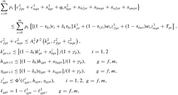 {\small{\begin{eqnarray*}
&&\sum _{t=0}^{\infty }p_{t}\left\lbrace c_{fpt}^{1}+c_{mpt}^{1}+x_{kpt}^{1}+q_{t}x_{kpt}^{2}+x_{hfpt}+x_{hmpt}+x_{\eta fpt}+x_{\eta mpt}\right\rbrace \nonumber \\
&&\qquad \le \sum _{t=0}^{\infty }p_{t} \left\lbrace \left[(1-\tau _{kt})r_{t}+\delta _{k}\tau _{kt}\right]k_{pt}^{1}+(1-\tau _{\ell ft})w_{t}z_{fpt}^{1}+(1-\tau _{\ell mt})w_{t}z_{mpt}^{1}+T_{pt}\right\rbrace , \nonumber \\
&&c_{fpt}^{2}+c_{mpt}^{2}\le A_{t}^{2}F^{2}\left(k_{pt}^{2},z_{fpt}^{2}+z_{mpt}^{2}\right), \nonumber \\
&&k_{pt+1}^{i}\le \left[(1-\delta _{k})k_{pt}^{i}+x_{kpt}^{i}\right]/(1+\gamma _{p}),\qquad i=1,2 \nonumber \\
&&h_{gpt+1}\le [(1-\delta _{h})h_{gpt}+x_{hgpt}]/(1+\gamma _{p}),\qquad g=f,m, \nonumber \\
&&\eta _{gpt+1}\le [(1-\delta _{\eta })\eta _{gpt}+x_{\eta gpt}]/(1+\gamma _{p}),\qquad g=f,m, \nonumber \\
&&z_{gpt}^{i}\le \Phi ^{i}(\ell _{gpt}^{i},h_{gpt},\eta _{gpt}),\qquad i=1,2,\ g=f,m, \nonumber \\
&&\ell _{gpt}=1-\ell _{gpt}^{1}-\ell _{gpt}^{2},\qquad g=f,m, \nonumber
\end{eqnarray*}}}
{\small{\begin{eqnarray*}
&&\sum _{t=0}^{\infty }p_{t}\left\lbrace c_{fpt}^{1}+c_{mpt}^{1}+x_{kpt}^{1}+q_{t}x_{kpt}^{2}+x_{hfpt}+x_{hmpt}+x_{\eta fpt}+x_{\eta mpt}\right\rbrace \nonumber \\
&&\qquad \le \sum _{t=0}^{\infty }p_{t} \left\lbrace \left[(1-\tau _{kt})r_{t}+\delta _{k}\tau _{kt}\right]k_{pt}^{1}+(1-\tau _{\ell ft})w_{t}z_{fpt}^{1}+(1-\tau _{\ell mt})w_{t}z_{mpt}^{1}+T_{pt}\right\rbrace , \nonumber \\
&&c_{fpt}^{2}+c_{mpt}^{2}\le A_{t}^{2}F^{2}\left(k_{pt}^{2},z_{fpt}^{2}+z_{mpt}^{2}\right), \nonumber \\
&&k_{pt+1}^{i}\le \left[(1-\delta _{k})k_{pt}^{i}+x_{kpt}^{i}\right]/(1+\gamma _{p}),\qquad i=1,2 \nonumber \\
&&h_{gpt+1}\le [(1-\delta _{h})h_{gpt}+x_{hgpt}]/(1+\gamma _{p}),\qquad g=f,m, \nonumber \\
&&\eta _{gpt+1}\le [(1-\delta _{\eta })\eta _{gpt}+x_{\eta gpt}]/(1+\gamma _{p}),\qquad g=f,m, \nonumber \\
&&z_{gpt}^{i}\le \Phi ^{i}(\ell _{gpt}^{i},h_{gpt},\eta _{gpt}),\qquad i=1,2,\ g=f,m, \nonumber \\
&&\ell _{gpt}=1-\ell _{gpt}^{1}-\ell _{gpt}^{2},\qquad g=f,m, \nonumber
\end{eqnarray*}}}
where we follow the same notational convention as in the previous section. The function mapping, Φ, hours and human capital into effective labor is indexed by the type of activity. This specification allows for different skills for the production of market goods and nonmarket goods (for example, computer programming and child rearing). In addition, it allows us to consider the effects of differential productivity between females and males in the production of some goods. We denote by kipt the amount of capital devoted to activity i, i = 1, 2. Note that these should be thought of as broad measures of capital goods—for example, including all appliances, autos, and the house itself in the production of the home good. Correspondingly, we want to allow for the relative prices of home capital goods to fall over time, so qt denotes the relative price of a home capital good in period t. The price of consumption in period t is given by pt. The real wage rate is wt, and the rental rate is rt. Finally, γp is the rate of population growth, and Tpt is transfers.Footnote 4
The terms τℓgt capture, as before, the tax rates on the labor services of a married individual of gender g. In this aggregate model, this wedge between women’s and men’s wages is meant to capture both outright discrimination and other factors (for example, marriage bars, career tracking, glass ceilings, or changes in the shadow price of characteristics) that result in lower effective wages for women. This wedge is important because it is the after-tax wage rate that will determine the pay-off to investment in human capital. Substantial differences can be seen between the raw wage gap—which is our driving shock—and the adjusted wage gap, which corresponds to what is measured in the data. The latter includes not only the differences captured by (1 − τℓft)/(1 − τℓmt), but also other differences in characteristics (human capital), both measured and unmeasured that—although endogenous—vary systematically across groups. We assume that labor tax rates do not depend on marital status.
The problem solved by single women (indicated by the subscript fs) and single men (subscript ms) are similar to (2), with the obvious changes.
Let ngs be the number (fraction) of individuals of gender g (f or m) who are single, and let np be the number (fraction) of partnerships. For simplicity, we will assume that these variables do not change over time. A bar over a variable denotes an economy-wide average. Thus,
 \[
\bar{k}_{t}^{1}=n_{fs}k_{fst}^{1}+n_{ms}k_{mst}^{1}+n_{p}k_{pt}^{1}
\]
\[
\bar{k}_{t}^{1}=n_{fs}k_{fst}^{1}+n_{ms}k_{mst}^{1}+n_{p}k_{pt}^{1}
\]
denotes the aggregate supply of capital, and
 \[
\bar{z} _{t}^{1}=n_{fs}z_{fst}^{1}+n_{ms}z_{mst}^{1}+n_{p}(z_{fpt}^{1}+z_{mpt}^{1})
\]
\[
\bar{z} _{t}^{1}=n_{fs}z_{fst}^{1}+n_{ms}z_{mst}^{1}+n_{p}(z_{fpt}^{1}+z_{mpt}^{1})
\]
denotes the aggregate supply of effective labor.
We assume that there is a constant returns to scale (CRS) aggregate production function of market goods given by  $A_{t}^{1}F^{1}(\bar{k}_{t}^{1},\bar{z} _{t}^{1})$. Unless otherwise specified, we assume that both A 1t and A 2t grow at the exogenous rate γA. Feasibility in the goods market requires that
 \begin{eqnarray*}
&\!&n_{pt}\left[c_{pt}^{1}+x_{kpt}^{1}+q_{t}x_{kpt}^{2}+x_{hfpt}+x_{\eta fpt}+x_{hmpt}+x_{\eta mpt}\right] \nonumber \\
&&\qquad \qquad +n_{ms}\left[c_{mst}^{1}+x_{kmst}^{1}+q_{t}x_{kmst}^{2}+x_{hmst}+x_{\eta mst}\right] \nonumber \\
&&\qquad \qquad +n_{fs}\left[c_{fst}^{1}+x_{kfst}^{1}+q_{t}x_{kfst}^{2}+x_{hfst}+x_{\eta fst}\right]+G_{t}\le A_{t}^{1}F^{1}\left(\bar{k}_{t}^{1},\bar{z}_{t}^{1}\right), \nonumber
\end{eqnarray*}
\begin{eqnarray*}
&\!&n_{pt}\left[c_{pt}^{1}+x_{kpt}^{1}+q_{t}x_{kpt}^{2}+x_{hfpt}+x_{\eta fpt}+x_{hmpt}+x_{\eta mpt}\right] \nonumber \\
&&\qquad \qquad +n_{ms}\left[c_{mst}^{1}+x_{kmst}^{1}+q_{t}x_{kmst}^{2}+x_{hmst}+x_{\eta mst}\right] \nonumber \\
&&\qquad \qquad +n_{fs}\left[c_{fst}^{1}+x_{kfst}^{1}+q_{t}x_{kfst}^{2}+x_{hfst}+x_{\eta fst}\right]+G_{t}\le A_{t}^{1}F^{1}\left(\bar{k}_{t}^{1},\bar{z}_{t}^{1}\right), \nonumber
\end{eqnarray*}
where Gt denotes government spending on goods and services. We assume that Gt is a constant fraction of market output.
Definition. An equilibrium is a collection of prices [{pt}, {rt}, {wt}] and an allocation (defined as all quantities indexed by type of good, sex, and marital status) for which
1. Given prices, the allocation solves (2) and the equivalent problems for singles.
2. The allocation is feasible.
The model we just outlined is too complex to derive interesting quantitative results theoretically. To make some progress in understanding the effects of changes in technology and wage discrimination, we use standard numerical techniques to compute equilibrium allocations.Footnote 5
3.1. Functional Forms and Parameter Choices
We start with the specification of the functional forms we will use in our quantitative analysis. We consider the class of preferences given by Uf = Um = U, where
 \begin{equation*}
U={\frac{1}{1-\sigma }}\left[ \left( \psi _{1}(c^{1})^{\psi _{2}}+(1-\psi _{1})(c^{2})^{\psi _{2}}\right) ^{(1-\psi _{3})/\psi _{2}}(1-\ell ^{1}-\ell ^{2})^{\psi _{3}}\right] ^{1-\sigma }.
\end{equation*}
\begin{equation*}
U={\frac{1}{1-\sigma }}\left[ \left( \psi _{1}(c^{1})^{\psi _{2}}+(1-\psi _{1})(c^{2})^{\psi _{2}}\right) ^{(1-\psi _{3})/\psi _{2}}(1-\ell ^{1}-\ell ^{2})^{\psi _{3}}\right] ^{1-\sigma }.
\end{equation*}
The production function of both types of goods (market and nonmarket) are assumed to be Cobb–Douglas, with the same coefficients for market and nonmarket goods: Fi(k, z) = Aik θz 1 − θ, i = 1, 2. We assume that the production functions of specific human capital are identical across all categories (sex and marital status) and are given by Φi(h, η, ℓi) = (h)κi(η)ζiℓi, i = 1, 2.
The parameter choices for our benchmark case are shown in Table 1. We set np to match the fact that roughly 60% of the relevant U.S. population was married during the period we study. Values for government spending and tax rates on labor and capital are average U.S. postwar values. The annual growth rates γp and γA are long-run U.S. trend levels. The discount factor is chosen so that the trend interest rate is 4%.
Table 1. Benchmark parameter values
 ${}^\dagger \ U(c^1,c^2,\ell ) = {1\over 1-\sigma }\Big[(\psi _1(c^1)^{\psi _2}+(1-\psi _1) (c^2)^{\psi _2})^{(1-\psi _3)\over \psi _2} \ell ^{\psi _3}\Big]^{1-\sigma }$
Values for the capital share, θ, the rate of physical depreciation, δk, and two critical preference parameters, ψ2 and σ, are the maximum likelihood estimates of McGrattan, Rogerson and Wright (Reference McGrattan, Rogerson and Wright1997) for a model with home production. We set the depreciation rates for human capital, δh and δη, equal to the depreciation rate for physical capital, δk, for our benchmark example. Since good estimates for human capital rates are not readily available, these parameter choices will be one focus of our sensitivity analysis.
We choose the remaining preference parameters (ψ1, ψ3, λf), two of the elasticities for effective labor (κ1, κ2), and the paths of technology and discrimination taxes to achieve several objectives. First, with no change in technology or discrimination, we want the benchmark parameters to yield initial hours of work that match the 1950 hours in Figure 1A for three groups—married women, married men, and single women—and to yield a relative wage of 51%—which is the value we obtain from extrapolating back the time series in Figure 1B.Footnote 6 Second, we assume that the initial leisure of married men is equal to the initial leisure of married women. This determines a value for the weight on married women’s utility, λf. This weight turns out to be very low, only 0.062. Because this value is so low, it will be one of the parameters that we focus on when we do sensitivity analysis.
A third objective is to match the U.S. time series on relative wages (Figure 1B) in the benchmark simulation with a change in discrimination. To do this and achieve the initial conditions above, we set the initial discrimination tax,  $\tau _{d\,\scriptstyle {1950}}$, at 22% and set subsequent rates so that the model yields the same time path for relative wages as in Blau (Reference Blau1998) (see Figure 1B).
For the benchmark parameterization, we do not distinguish between type-h and type-η human capital; therefore, we assume that κi = ζi in both sectors, i = 1, 2. We experiment later by assuming no human capital and assuming sector-specific human capital.Footnote 7
We assume that the government purchases 20% of market goods and services and redistributes, in a lump-sum fashion, any remaining revenue generated. We interpret τℓmt as the governmentally specified tax rate on labor income and assume that any difference arising from discrimination is completely used for redistributive purposes. For simplicity, we assume that this redistribution is equally divided among all agents in the economy. This is consistent with our assumption that although we have modeled discrimination as a tax, it is not being used for revenue generation. Later, we look at alternative specifications of the distribution of revenue.
Finally, since we want to abstract from business cycle frequency effects, we consider a time period in our model to be five years. Thus, t = 0 corresponds to the year 1950, and t = 10 corresponds to the year 2000. The calculations that we perform assume that all agents perfectly anticipate the changes that are forthcoming.
For each experiment, we include sensitivity analyses on our results. The parameters used for these alternatives are included in Table 2.
Table 2. Numerical experiments

4. BACKGROUND DATA
In this section, we outline the basic facts about (i) U.S. labor supplies, (ii) relative wage rates, (iii) home capital goods prices, and (iv) home capital shares and compare these facts with our model solutions.
Notable changes here are the changes in the levels and composition of hours allocated to market production by sex and marital status that have occurred since 1950. In Figure 1A, we plot market hours of work per week for men and women, both married and single [see McGrattan and Rogerson (Reference McGrattan, Rogerson and Rupert2008) for details on construction of these time series]. The most striking facts are that the average number of hours worked by married women increased 209% from 8.0 to 24.7 hours per week between 1950 and 2000 and then stayed roughly constant. Between 1950 and 2000, the average number of hours worked by married men decreased from 41.7 to 38.8 ( − 7%). In contrast, the average number of hours worked by single individuals—both women and men—has been relatively stable, with single men working slightly more than single women. Finally, we can see a change in the relative composition of hours by a married couple, with the sum looking more and more like the sum of a single woman and a single man over the period (based on the average for those aged 25–64 years). More precisely, an artificial household formed by two single individuals worked approximately 60 hours per week in 1950 and in 2000. On the other hand, the average married couple worked approximately 50 hours per week in 1950, but almost 64 hours per week in 2000. These are the observations that we want the model to match as outputs.
The evidence on the size and nature of the gender wage gap has been well documented [see Goldin (Reference Goldin1990, Reference Goldin, Blau and Ehrenberg1997)]. For example, Blau (Reference Blau1998) finds that women working full-time earned about 56% of what men earned in 1969 and that this ratio was relatively flat until the mid-1970s and then rose to about 72% by 1994. Her estimates are plotted in Figure 1B.Footnote 8 The same pattern is seen for high school graduates and college graduates. The gender wage gap is a difficult measure to interpret. In principle, it can measure either the direct effects of wage discrimination (the payment of lower wages to one group despite equivalent training and work duties) or differences in unmeasured (by the econometrician) skills that are correlated with sex. These differences in skills themselves could be a result of discrimination [for example, glass ceilings and marriage bars; see Goldin (Reference Goldin1990)] or a result of other, nondiscriminatory, incentives for the development of skills across the sexes (for example, specialization in the provision of home goods and child care).
We model the gender wage gap as arising from two distinct sources. The first is wage discrimination in employment, which we model as a sex-specific tax. This modeling choice is similar to the formulation implied by the Becker (Reference Becker1971) approach to discrimination and can also be interpreted as the shadow price on sex-specific constraints on job types (for example, marriage bars or glass ceilings). The second source of wage differences in the model is differences, by sex, in skills (that is, human capital). Differences by sex in the attainment of these skills are endogenous to the model. The forces driving these differences arise partly from discrimination and partly from specialization within a married couple. For us, the lessening of the gender wage gap seen in the data comes from a reduction in this sex-specific tax rate.
Knowing the exact magnitude of the discrimination tax or how much it has changed is difficult, but Goldin (Reference Goldin1990) carefully documents several discriminatory practices and the beginning of their decline in the 1950s. Other relevant considerations include the passage of the 19th Amendment to the U.S. Constitution in 1920 that gave women the right to vote, the introduction of specific federal regulations against discrimination by sex [for example, the creation of the Equal Employment Opportunity Commission; see Goldin (Reference Goldin1990)], which would have an effect on wage payments by sex in either the Becker (Reference Becker1971) or the Coate and Loury (Reference Coate and Loury1993) models of discrimination, and the reduction in union power over the period, which would reduce the amount of effective discrimination in the Becker (Reference Becker1971) model. Since we know of no direct measures of the size of the relevant tax rate, we will do considerable experimentation below.
Likewise, direct measures of changes in productivity in the home are not easily obtainable. In the special case that increased productivity is realized as cheaper home capital, one part of the evidence is carefully discussed by Greenwood, Seshadri and Yorukoglu (Reference Greenwood, Seshadri and Yorukoglu2005). They document that the real price of household appliances decreased at an annual rate between 3.5% and 8.0% starting in 1950. They ignore other important categories of home capital, however. Some of these categories, such as autos, are also important time-saving durables used in home production and have had less dramatic price reductions. Housing itself has had virtually no real price reduction.
Figure 2A shows the time series of price deflators from the U.S. national income and product accounts for both broad and narrow measures of home capital. Durable consumption and residential investment represent about 8% and 4%, respectively, of GDP on average over the 1929–2010 period. In Figure 2A, we plot the weighted price deflator—with a two-thirds weight on durable consumption and a one-third weight on residential investment—which shows a decline over the period. However, the decline is not as dramatic as that in the price index of the other, more narrowly defined, category of household appliances. The category of household appliances represents about 0.6% on average over the 1929–2010 period and shows a marked decrease in prices over the period, with its value in 2010 about 20% of that in 1950.

Figure 2. U.S. hours and wage ratios since 1950. A. Ratio of home investment deflators to GDP deflator (1950 = 100). B. Home investment expenditure shaers (1950 = 100).
Figure 2B shows the time series of expenditure shares for the broad and narrow categories of home capital. The expenditure share for the durable consumption and residential investment category shows very little change over the period but moves systematically with the cycle. After a short post-World War II boom, the expenditure share of household appliances drops quickly, returns to its prewar level, then shows a slow, gradual decline over the next 35 years.
5. TECHNOLOGICAL CHANGE IN THE HOME
In this section, we study the impact of changes in technology on the allocation of labor by singles and partnerships. We could, in principle, study the effects of technological change in the model outlined above in many ways. We could assume sector-specific growth rates in market and home activities, for example. Although we do discuss this alternative in the section on sensitivity below, one problem is the lack of direct measurement of the rate of technological change in the home sector. Thus, we focus first on the effect discussed by Greenwood, Seshadri and Yorukoglu (Reference Greenwood, Seshadri and Yorukoglu2005), that the price of durables in the home sector has fallen over the period we are studying.Footnote 9 Correspondingly, we ask, What is the equilibrium effect of reductions in q in the budget constraint of the individual households?
A popular explanation for the increase in hours allocated to market work is that improvements in household durables and in the availability of ready-made goods (for example, clothes and foodstuffs) free up time from housework. From a theoretical point of view, this is not necessarily the case, as was shown in Section 2. Increases in productivity can increase or decrease the hours allocated to housework depending on the elasticity of substitution between home and market goods. From an empirical perspective, the evidence is mixed. Using evidence from a number of time-use data studies, historians of technology [for example, Cowan (Reference Cowan1983)] argue that substantial increases in the productivity of labor allocated to home production did not result in decreases in the number of hours of housework, especially during the 1870–1940 period, which may have seen the largest productivity increases. The unchanging home work hours, despite increased productivity, could have occurred because of increases in the quantity or quality of home good production (for example, washing clothes more often or housecleaning more thoroughly) or from changes in demands for doing this work (for example, moving to the suburbs or purchasing a larger house). Economic historians, such as Mokyr (Reference Mokyr2000), agree with the facts presented by Cowan (Reference Cowan1983), but differ in their interpretation. Mokyr (Reference Mokyr2000) argues that several scientific revolutions have induced households to spend more time on housework in order to increase the quality of home production. Greenwood, Seshadri and Yorukoglu (Reference Greenwood, Seshadri and Yorukoglu2005) argue that the diffusion of household durables can account for the increase in women’s labor force participation.
To give this explanation the best chance for success, we use the same change in q as that used by Greenwood, Seshadri and Yorukoglu (Reference Greenwood, Seshadri and Yorukoglu2005), that given by appliance prices, a reduction of 77% over the 1950–1990 period, the period marking a dramatic rise in hours of work for married women. As noted above, this reduction in prices is much more dramatic than what is seen in other household durables (for example, autos and houses themselves) and is similar in magnitude to the reduction of some narrowly defined classes of producer durables.
5.1. Results
The results of our computations are shown in Figure 3. As noted above, the best estimates are that home and market goods are substitutes, but in this case, a reduction in q actually causes married women’s market hours to fall, in contrast to what is seen in the data. Because of this, we focus on examples in which home and market goods are complements.

Figure 3. Predictions of model with falling home capital price. A. Market hours of work per week. B. Ratio of women’s to men’s wage rates (%). C. Ratio of home investment to market output (1950 = 100).
The hours series for one of these examples (with ψ2 = −0.75) is shown in Figure 3A. As can be seen, the experiment is successful for single households; the hours of both single women and single men are unchanged in response to the price reduction. The experiment is not successful for married households, however. The effect on married women’s market hours is measurable, but it is much smaller than the increase in hours seen in the data. Similarly, the change in married men’s hours is hardly noticeable, again in contrast to what is seen in the data.
Even though human capital is allowed to adjust in response to the fall in q, it does not. Therefore, the relative wage of women and men is unchanged. Again, this finding is in contrast to what is seen in the data, and it is shown in Figure 3B.
Figure 3C shows the time path for expenditure shares on home capital. In contrast to the data, this share increases significantly and stays high.
In sum, the prediction of the model is that in response to the change in the price of durables, hours in the home stay roughly unchanged, as do human capital investment decisions. A dramatic increase in k 2 takes place, however, mirroring the discussion of our simple example. This change can be thought of as an increase in either the quantity or the quality of the durables used to produce home goods.
5.2. Sensitivity Analysis
Table 3 displays the numerical results for the example discussed above (in the second row of numbers) along with the results of several other related experiments. The third row of Table 3 shows the results for an example with even less substitution, ψ2 = −4. In this case, married women’s hours increase more, by 4.7 hours per week between 1950 and 2000, but still significantly less than the 16.7 hours per week in the data. For married men, the change is 1 hour per week, similar in magnitude to the 0.7 hours seen above, whereas in the data the corresponding change is 2.9 hours. Not shown in the table are the results of experiments based on more inclusive notions of home capital goods. Since in those experiments, the corresponding reduction in q is smaller, even smaller changes in hours result.
Table 3. Effects of changes in home technology‡

‡ MF = married females, MM = married males, SF = single females, SM = single males.
An alternative way of studying the impact of improvements in home technologies is to study the effects of increases in A 2 over and above any general technical change. In order for this alternative to have a chance at being successful, however, preferences must deviate substantially from the power utility case. In the power utility case, an increase in A 2t, to say  $\hat{A}^2_t=(1+\gamma )A^2_t$, raises home consumption by a factor γ but leaves all other variables, including hours of work, unchanged.Footnote 10 This theoretical result implies that, by continuity, changes in the home technology for any specification of preferences near unitary elasticity of substitution between home and market goods must necessarily result in a small effect on hours. As such, it serves as a useful benchmark for what follows.
Here, as above, we investigate what happens only when home and market goods are complements, since if they are substitutes, market hours actually fall. To generate the large changes in hours worked by married women observed in U.S. data, we are forced to examine very large changes in the value of A 2. The results are displayed in Table 3. Again, with ψ2 = −0.75, the size of the change in A 2 that is needed to match the data is to increase it from A 2 = 1.0 to A 2 = 5.0, over and above our benchmark level of technological change. With our benchmark growth rate in the market sector of γA = 2%, this corresponds to a growth rate in home productivity of over 5% per year, whereas market productivity grows at only 2% per year.
Although this simulation matches the hours data well, with only a small change by singles, it has three problems. First, for this story to be successful, home and market goods must be complements, contrary to best estimates. Second, very large changes in technology are required changes, over and above those measured in market productivities. Finally, even in these cases, we see only small effects on the observed wage gap. This last point is important, since it is directly related to changes in human capital formation decisions, and as pointed out above, a dramatic shift in the schooling decisions of men and women seems to have taken place during the last 60 years.
Our results contrast with those of Greenwood, Seshadri and Yorukoglu (Reference Greenwood, Seshadri and Yorukoglu2005). There are two key differences. First, Greenwood, Seshadri and Yorukoglu (Reference Greenwood, Seshadri and Yorukoglu2005) assume that the labor supply decision is indivisible. Thus, married women are prevented from working part-time. This assumption implies that the elasticity of substitution between home and market goods plays no role in their model. If a household is sufficiently productive, then a decrease in the price of a durable that results in adoption on the part of a household frees up time—the technology is Leontief—that can only be used to produce either market goods or leisure.
Second, since Greenwood, Seshadri and Yorukoglu (Reference Greenwood, Seshadri and Yorukoglu2005) assume that the home technology is Leontief, and there are only two options for producing in the home, utility effectively exhibits satiation in the home good in their formulation. This seems to be why their model predicts that married women’s participation will eventually begin to fall and durables expenditures decline as a fraction of GDP. As we shall see in the next section, this is the driving force behind their results.
6. INFERIORITY OF THE HOME GOOD
Another explanation for the observed change in married women’s hours is that the home good is inferior. This, when accompanied by overall income growth, can cause married women’s home hours to fall, freeing up time for more work in the market. In a static setting, a change in income could cause relatively more effort to be directed at obtaining market goods and relatively less at home goods. This suggests that observed changes in hours might be due to income growth, as seen in the United States in the presence of inferiority of the home good. This is the hypothesis we study in this section.
We examine two variations on the model above, where the utility function includes inferiority of the home good. The functional forms that we examine are
 \begin{eqnarray*}
\vspace{-10.0pt}V_{1}(c^{1},c^{2})&=&(\psi _{1}(c^{1})^{\psi _{2}}+(1-\psi _{1})(c^{2})^{\alpha \psi _{2}})^{(1-\psi _{3})/\psi _{2}}, \ \mathrm{with\ } \alpha \le 1, \nonumber \\
V_{2}(c^{1},c^{2})&=&\left\lbrace \begin{array}{ll}(\psi _{1}(c^{1})^{\psi _{2}}+(1-\psi _{1})(c^{2})^{\psi _{2}})^{(1-\psi _{3})/\psi _{2}}& \text{if } c^{2}<c^{\ast },\\
(\psi _{1}(c^{1})^{\psi _{2}}+(1-\psi _{1})(c^{\ast })^{\psi _{2}})^{(1-\psi _{3})/\psi _{2}}& \text{if } c^{2}>c^{\ast }, \end{array}\right. \nonumber
\end{eqnarray*}
\begin{eqnarray*}
\vspace{-10.0pt}V_{1}(c^{1},c^{2})&=&(\psi _{1}(c^{1})^{\psi _{2}}+(1-\psi _{1})(c^{2})^{\alpha \psi _{2}})^{(1-\psi _{3})/\psi _{2}}, \ \mathrm{with\ } \alpha \le 1, \nonumber \\
V_{2}(c^{1},c^{2})&=&\left\lbrace \begin{array}{ll}(\psi _{1}(c^{1})^{\psi _{2}}+(1-\psi _{1})(c^{2})^{\psi _{2}})^{(1-\psi _{3})/\psi _{2}}& \text{if } c^{2}<c^{\ast },\\
(\psi _{1}(c^{1})^{\psi _{2}}+(1-\psi _{1})(c^{\ast })^{\psi _{2}})^{(1-\psi _{3})/\psi _{2}}& \text{if } c^{2}>c^{\ast }, \end{array}\right. \nonumber
\end{eqnarray*}
with  $U={\frac{1}{1-\sigma }}[(V_{i}(c^{1},c^{2}))^{1-\psi _{3}}(1-\ell ^{1}-\ell ^{2})^{\psi _{3}}]^{1-\sigma }$, i = 1, 2. Thus, when α = 1, V 1 is like our benchmark model, but when α < 1, the function is more concave in the home good than in the market good. The utility function V 2 is even more extreme with strict satiation in the home good.
We also examine two different sources of increases in wealth: trend growth in productivity and reductions in prices of capital goods. (The latter also induces important substitution effects.)
6.1. Results
We find that specifications like that in V 1 are not successful, no matter what the source of income growth is. This is true no matter how small we make α. It does not matter whether the source of growth is technological change overall or specific to some or all of the capital goods in the model. In all cases, the change in married women’s labor supply is inconsequential.
Whether specifications like those in V 2 work depends critically on the choice of c*. Here we have a delicate balancing act: if c* is chosen too low, home hours fall for all households, including singles, whereas market hours increase. This result is not what we see in the data. But if c* is too large, it has no effect on the market hours of any of the households. Within a specific range of values for c*, the effect on married couples is large, but the effect on singles is small.
The hours series for one such example are shown in Figure 4A. Here, we assume that capital prices are unchanged, but overall productivity grows as in our benchmark parameterization. The increase in the hours of both married women and married men lines up quite well with the data. The same is true for singles, both women and men.

Figure 4. Predictions of model with inferior home goods. A. Market hours of work per week. B. Ratio of women’s to men’s wage rates (%). C. Ratio of home investment to market output (1950 = 100).
This example has three weaknesses, however. Primarily, it requires exactly the right specification of satiation (that is, c*) to match the facts. It is difficult to know whether this specification is realistic, and we know of no independent way of corroborating it. Another weakness is that although the hours data match up well, even this extreme version underpredicts the level of the observed wage gap between 1970 and 1995 (Figure 4B). Finally, as one might guess, one implication that accompanies this specification is that the share of home investment goods in output drops drastically, to below 40% of the 1950 level by 2010. Figure 4C shows the time series from the model along with that in the data, where the share in output is roughly constant over time.
6.2. Sensitivity Analysis
We conduct numerous sensitivity analyses of the examples described above in an attempt to isolate the relative contributions of different sources of income growth and preference specification. We find that any of the sources of income growth produce only small effects when the utility function is of the type in V 1. In contrast, when utility is given by the form in V 2, durables prices alone produce almost no effect without overall growth in productivity. Similarly, when durables price reductions are added to the model with productivity growth, again, the marginal effect is quite small. Thus, we conclude that any effect that is present with this specification is present only when we have both strict satiation and overall productivity growth. The declining price of durables seems to play only a minor role.
7. FEMALE–MALE WAGE DIFFERENTIALS
In this section, we study the impact of changes in measures of sex-specific distortions—given by (1 − τdt) = (1 − τℓft)/(1 − τℓmt)—on labor supply decisions. Substantial evidence indicates that, even after controlling for a number of measurable characteristics, women’s wages are lower than men’s [see, for example, Goldin (Reference Goldin1990), Blau and Kahn (Reference Blau and Kahn1997) and Blau (Reference Blau1998)]. Moreover, the data indicate that this gap has been narrowing in the last few years.
Given the specification that we have chosen, it follows that the gap in wages of women relative to men is given by
 \begin{equation*}
\ln \left( \frac{w_{ft}}{w_{mt}}\right) =\ln \left( \frac{1-\tau _{\ell ft}}{ 1-\tau _{\ell mt}}\right) +\kappa _{1}\ln \left( \frac{h_{ft}}{h_{mt}} \right) +\zeta _{1}\ln \left( \frac{\eta _{ft}}{\eta _{mt}}\right)\!.
\end{equation*}
\begin{equation*}
\ln \left( \frac{w_{ft}}{w_{mt}}\right) =\ln \left( \frac{1-\tau _{\ell ft}}{ 1-\tau _{\ell mt}}\right) +\kappa _{1}\ln \left( \frac{h_{ft}}{h_{mt}} \right) +\zeta _{1}\ln \left( \frac{\eta _{ft}}{\eta _{mt}}\right)\!.
\end{equation*}
Hence, this gap is made up partly from the direct effects of the distortion τdt and partly from the indirect effects of different human capital accumulation decisions.
Recall that in the U.S. data, wft/wmt rose from about 56% in 1969 to about 72% in 1994. If all relevant skills (that is, h and η) were perfectly measured and controlled for, we would have direct measures of both the level and the change in 1 − τdt that must have occurred over this time period. If, however, h represents skills measured by the econometrician (for example, years of schooling), while η represents other skills that are not adequately measured (for example, ability to use spreadsheet software), and if these unmeasured skills differ systematically by sex, then wft/wmt would be an overestimate of 1 − τdt. Moreover, the change in wft/wmt would be an overestimate of the true change in discrimination if ηf/ηm increases when τd falls.
We study a version of the model in which the series τdt is calibrated so that the model and Blau’s (Reference Blau1998) estimates for the relative wages of women and men match. This series necessarily requires that the value of τdt fall over the time period. To match the observed series of relative wages, we assume a tax rate on women of τℓft = 0.40 in 1950 (for comparison, recall that τℓmt = 0.23), and we assume that this rate falls to τℓft = 0.35 by 1995, where it stabilizes.Footnote 11 This gives an initial discrimination tax of  $\tau _{d\,\scriptstyle {1950}}\!=\!1\!-\!(1\!-\!\tau _{\ell f\,\scriptstyle {1950}})/ (1\!-\!\tau _{\ell m\,\scriptstyle {1950}})=0.22$, and a later value of $\tau _{d\,\scriptstyle {1995}}=0.16$. Since we do not have a direct measure of the τdt series, we will conduct considerable experimentation on it below.
7.1. Results
Figure 5B shows the time path of relative wages as given by Blau (Reference Blau1998) (and extended to include an estimate for 2009), along with that calculated from our model. The predictions of the model for the number of hours worked and the comparable values for the United States are presented in Figure 5A. The model prediction matches the long-run behavior of married women’s hours worked very accurately, both the change from steady state to steady state and the path over the last 60 years. Note also that the response by single women to the same change in discrimination over the period 1950–2000 is significantly smaller. Large changes in discrimination are not needed to mimic these patterns of hours worked. Indeed, the time path of women’s hours in the data is exactly what one would expect from a relatively small change in discrimination.

Figure 5. Predictions of model with changes in discrimination. A. Market hours of work per week. B. Ratio of women’s to men’s wage rates (%). C. Ratio of home investment to market output (1950 = 100).
Several features of the model are, however, at odds with the data. The hours series from the model for married men is very accurate over the period 1950–1980, but the predictions fall slightly below the actual series at the end of the sample. The hours series from the model for single men is systematically too high throughout the 1950–1980 period. The model outcome for single men shows a small but significant downward trend, whereas in the data, these hours are U-shaped.
The small change in market hours for singles over the 1950–1990 period that the model generates is in keeping with the discussion of the static model in Section 2. Thus, the qualitative behavior predicted there with logarithmic preferences continues to hold (approximately) in this dynamic setting even though the static elasticity of substitution between home and market goods is 1.67 and not 1.
The fact that hours in home production are roughly equal for single women and single men and constant over the experiment is directly reflected in the time paths for home consumption, which are also roughly equal and quite stable. This is also in keeping with the static example.
Although not shown here, the behavior of market consumption is more complex. Over time, single women’s market consumption rises roughly in step with the reduction in effective labor tax rates over the period, a prediction of the static model. However, that is not true for the relationship between single women’s and single men’s market consumption. Here, the static model would suggest that the ratio of market consumptions between the two types of single agents would be equal to the ratio of their tax rates. In fact, single women consume less than this. The main reason is that the existence of discrimination induces a difference in human capital investment that exaggerates the differences in wages and, hence, the differences in consumption. This is a purely dynamic effect of discrimination.
Is the increase in married women’s hours in the market at the cost of hours spent in leisure or in home production? As it turns out, the answer to this question is both: about 33% comes from reduced leisure, and 67% comes from reduced work in the home. Indeed, in part because of our assumption that leisure for the two partners is equal in 1950, by 1990 married women are working outside the home approximately nine hours more per week in total than are married men.
As a final point on the equilibrium hours series produced by the model, note that, as discrimination is reduced, a married couple looks more and more like a single woman and single man. That is, as can be seen in Figure 5A, although total market hours for a married couple are substantially fewer than those for two singles at the beginning of the period (50 hours versus 60 hours), they are roughly the same by 1995. This is true in the data as well. This phenomenon is a by-product of the reduced incentives for overconsumption of the home good as a tax avoidance strategy by the married couple.
Since this version of the model is successful at matching the hours series, we are led to examine its other predictions. One interesting feature of the model is its implications for decisions on human capital investment. It predicts a substantial difference across the sexes in the investment paths in human capital for both single and married agents. This difference is directly due to the increased rate of return on human capital accumulation for the woman arising from the forecast reduction in tax rates she faces. The time paths for human capital for all agents are shown in Figure 6A. Over time, the decrease in the gender wage gap induces women to invest more in human capital and less in physical capital. Thus, a portfolio reallocation effect is associated with changes in discrimination. The predicted increases are substantial. In 1950, the stock of married women is 35% of the level of married men and rises to nearly 65% by 2000. In 1950, the stock of single women is 48% of the level of married men and rises to nearly 60% by 2000. Men’s investment decreases somewhat, but only relative to trend; the absolute level does not fall. As we will see, some versions of the model predict that human capital of single women will overtake and pass that of single men about the time the discrimination tax hits zero. Interestingly, this result is similar to what has been seen recently; women’s college graduation rates in the United States have now surpassed those of men. In contrast, in the versions of the model in Sections 5 and 6, the changes in human capital by women are much smaller, with virtually no change in single women’s stocks.

Figure 6. Auxiliary predictions of model with discrimination. A. Human capital relative to married men in 1950. B. Ratio of single to married wage rate by sex (%). C. Average market productivity relative to trend (1950 = 100).
This change in human capital investment for women has implications for the composition of the stock of wealth for all agents in the economy. For a married couple, the share of human capital increases, whereas the share of physical capital decreases. This change is entirely internally financed by the couple, however, with virtually no change over the period in holdings of physical capital. For single women, investment in physical capital decreases dramatically, eventually becoming negative. This decrease, coupled with the increase in their investments in human capital, implies a substantial change in the composition of their portfolio. Single men behave in the opposite way. Thus, single women borrow in order to finance investment in human capital. In the model, this is accomplished by a decrease in investment in physical capital. Single men are on the other side of this market. For them, the rate of return on human capital has not increased, and they are willing to lend to single women.
The change in the incentives for human capital accumulation is the property of the model that drives the results on the paths of hours for women. As discrimination falls, wage rates for women would rise even in the absence of any increase in investment. The increased investment in human capital has two effects: it increases the size of the wage change and exaggerates the increase in the cost of leisure for women over the period of transition. These two effects induce intertemporal substitution of leisure along the transition path. Consequently, women choose to work relatively little early on and increase hours substantially over the period of transition.
The model also has implications for the marriage premium for both women and men. We define the female (male) marriage premium as the ratio of hourly wages between married and single women (men). These ratios are shown in Figure 6B. For men, the model predicts a reasonably large increase: wages of single men are about 3% less than married men in 1950, rising to more than 5% above by 2000 and remaining constant thereafter. In the data, this ratio is also fairly constant, but considerably lower, with wages of single men about 20% below those of married men. As expected, the differences in relative wages in the model are larger for women. In 1950, the ratio of wages of single women to those of married women is 1.17, and the ratio falls smoothly over the time period, reaching 0.97 by 1990. In the data, the corresponding values are 1.15 for 1970 (which is also the value from the model) and 1.02 for 1990. Thus, the model matches this feature of the data fairly well.
Finally, the model has implications for the time path of productivity for the economy. Some economists have argued that part of the productivity slowdown seen in the United States in the 1970s and early 1980s is due to the increase in women’s labor force participation [see Baily (Reference Baily1986)]. The intuition is straightforward. Because of both discrimination and specialization, women have lower skill levels than their male counterparts. Thus, women’s participation increases and average labor productivity falls. This argument misses the point that skill acquisition is endogenous, however. The overall effect, then, depends on which changes faster: women’s hours or their human capital. The time path of overall labor productivity in the model does indeed fall relative to trend, as this argument suggests (but in some parameterizations, it actually rises). Thus, the view that the observed path is due to increased participation by women is consistent with the model of reduced discrimination against women. This finding also points out that the reduction in productivity relative to trend may actually lead to a welfare improvement, at least for some groups.
7.2. Sensitivity Analysis
We turn now to the sensitivity of our results. Some of the modeling choices that we have made are standard; they have counterparts in all dynamic models (for example, discount factors and preference and production parameters). Others—the choice of welfare weights within a couple, the specification of effective labor including human capital, the nature of the transfer scheme for distributing the revenue raised by the discrimination tax, and the assumption of equal discrimination against married and single women—are unique to the questions that we are addressing. We find that generally speaking, our results are robust to alternative specifications. The one exception is the specification in which discrimination affects married women only; this example is difficult to match with the observed wage series.
Table 4 reports hours of work, relative wages, and home investment shares for several alternative versions of the model. The first row of numbers contains the U.S. data, and the remaining rows display statistics for the different model parameterizations, the first being the benchmark parameterization discussed above.
Table 4. Effects of fall in discrimination‡

‡ MF = married females, MM = married males, SF = single females, SM = single males.
In our benchmark case, the weight on married women’s utility is low (λf = 0.062). As indicated before, this is necessary in the benchmark example to keep total hours by the woman, home plus market, at the same level as those of her partner. The first experiment reported in Table 4 assumes a higher weight on women’s utility—the same, in fact, as that on married men’s. In order to match the wage series for this parameterization, a larger change in τd is required (see Table 2). In this experiment, we assume that  $\tau _{d\,\scriptstyle {2000}}=0.12$; hence, the reduction is still a relatively modest 10%. Given this assumption, however, the changes in hours are similar to those in the benchmark model.
In a second experiment, we consider a variation of the model with no human capital. Here, we set κi and ζi, i = 1, 2, equal to 0.001 so that the return to human capital is negligible. All other parameters are as in the benchmark example except for the path of τd, which begins at  $\tau _{d\,\scriptstyle {1950}}=0.48$ and falls to $\tau _{d\,\scriptstyle {2000}}=0.22$, as is required to match the wage series. In this case, it follows that the gap is simply the wedge introduced by the discrimination tax. No additional wedge is introduced by human capital differences. The smaller gap means that larger changes in discrimination are required to match the relative wage series, but beyond this, the results of the experiment are quite similar to the benchmark case. Thus, the role of human capital is quantitatively significant, in that with human capital included, only a 6% drop in τd is required, whereas without it, a drop of 26% is needed.
Also included in Table 4 are two further experiments on the role of human capital. In one, we assume that human capital is useful only in the market sector. In the other, we assume that the two types of human capital are sector-specific. The results are similar for all variations, with the exception of the path τd required to mimic the gender wage gap.
For the simulations discussed so far, we have assumed that revenues from the discrimination tax are lump-sum rebated in an equal per capita fashion. An alternative hypothesis is that the revenue raised from discrimination against women is used to subsidize some other group of agents. To analyze this possibility, we simulate a specification in which the revenues generated from the discrimination tax are used as a subsidy to married men [Goldin (Reference Goldin1990, p. 102)]. The parameters of the model are recalibrated to match initial hours and the time path of the wage gap. From this, we find that similar changes in the discrimination tax give nearly identical results, as our benchmark simulation does.
The benchmark simulation assumes equal discrimination against both married and single women. In fact, many of the discriminatory practices that have been documented [for example, marriage bars; see Goldin (Reference Goldin1990)] seem to exhibit more discrimination against married women. Because of this, we consider an example in which we set the discriminatory taxes for single women equal to zero, with the other parameters held fixed at their benchmark levels. This experiment is the last row in Table 4. Here, we can find no time path for τd that replicates the time series of the gender wage gap. Hence, we use the path from our benchmark parameterization. We find that this change significantly increases the relative wage of women in all periods and leads to more market hours in 1950 for all groups except married males. The reduction in discrimination, however, still creates a substantial increase in married women’s market hours, from 10.0 hours per week in 1950 to 26.3 in 2000.
In sum, the results reported in our benchmark example seem fairly robust to both changes in the parameters and the details of the treatment of the discrimination tax. As long as the levels and changes in τd are chosen to match the observed path of the gender wage gap, the pattern for hours is consistent with the data. The size and the change of τd that are needed for this depends critically on the role of human capital, however.
8. CONCLUSIONS
In this paper, we have examined three alternative hypotheses for the large changes over the postwar period in married female labor supply. These are: (i) the changes are a result of improvements in the technology for producing home goods, (ii) they follow from overall income growth if home goods are inferior, and (iii) they are a result of a reduction in the gender wage gap. Our results show that improvements in home technologies are not successful in accounting for the data. Some extreme forms of home good inferiority (satiation) do have limited success, but these forms bring with them a host of other, counterfactual, predictions. We find that a reduction in the gender wage gap is the most successful of the three. Since one possible reason for the observed change in the gender wage gap is a reduction in discrimination against women, our findings are consistent with the view that this is the driving force. Because of limitations in both the model and the data, however, our results are also consistent with changes in the gender wage gap that arise from sex-specific improvements in market productivity.
Changes in the wage gap do not have large effects on singles, given a specification in which income and substitution effects cancel out each other. This situation is characteristic of both single women and single men. For partnerships, however, there is another margin: endogenous specialization allows married women to partially avoid the discrimination tax. Thus, changes in the gap between women’s and men’s wages induce substantial reallocations within the family, even though overall changes in the level of wages have a small impact on labor supply. This result implies that married women respond to changes in discrimination by substantially changing their market hours.
Our results suggest that changes in the rate of productivity growth in the home production sector are not as successful in explaining the U.S. historical experience for two reasons. First, for hours of married women to increase, we need to assume that market and home goods are complementary, in contrast with the best estimates. Second, even in this case, to match the increases in the number of hours worked by married women, the model requires exceptionally large increases in the productivity of household activities. The impact of the declining relative price of home capital is found to be relatively minor, with the model predicting that this will be met with increases in the quantity and quality of home production. Similarly, stories based on the inferiority of home goods face difficulties. Even with the extreme versions of this specification that are needed to match the hours pattern, the model produces counterfactual predictions about expenditure shares on home durables. It also has difficulty in tracking the observed pattern of the gender wage gap.
We view our model of a time-changing discrimination tax as a first step. We have ignored the effects of uncertainty about returns to human capital and the permanence of marriage (divorce). In addition, we have taken the decision to form partnerships as exogenous. More work is needed to assess the impact of uncertainty about marital status on accumulation decisions and the effects of endogenizing the marriage decision. We conjecture that including these features will not change the basic conclusions we have reached here, but will improve the model’s overall fit, especially for the behavior of single households. This is because much of what is at odds with the data in the current version of the model comes from intertemporal trading between single women and men conducted under the assumption that marital status will not change. When this assumption is relaxed, we expect that the predicted downward trend in single men’s hours (for example) will largely disappear.
APPENDIX: GLASS CEILINGS AND JOB CHOICE
Here, we develop a simple model of job restrictions that are sex-specific and show that this is equivalent to the sex-specific tax τd described in the main text.
There is a continuum of job types, indexed by s ∈ S⊂R +. Each agent chooses one and only one job. There is an inelastic supply of hours, which is set without loss of generality at one per person. We assume that the relative productivity of a person working in job type s is φ(s). Thus, if n(s) is the number of workers of type s that a firm hires, output for that firm is given by
 \begin{equation*}
y=F\left(k,\int _{S}\varphi (s)n(s) ds\right).
\end{equation*}
\begin{equation*}
y=F\left(k,\int _{S}\varphi (s)n(s) ds\right).
\end{equation*}
Thus, a worker in a job of type s earns the wage w(s) = φ(s)F ℓ(k, ∫Sφ(x)n(x)dx).
Suppose that the disutility of working in a job of type s is given by v(s). Then, the problem for a typical male worker facing tax rate τ is given by
 \begin{equation*}
\max _{s}\quad (1-\tau )\varphi (s)F_{\ell }-v(s).
\end{equation*}
\begin{equation*}
\max _{s}\quad (1-\tau )\varphi (s)F_{\ell }-v(s).
\end{equation*}
The optimal choice of job for this male, sm, satisfies
 \begin{equation*}
(1-\tau )F_{\ell }\varphi ^{\prime }(s_m)=v^{\prime }(s_m).
\end{equation*}
\begin{equation*}
(1-\tau )F_{\ell }\varphi ^{\prime }(s_m)=v^{\prime }(s_m).
\end{equation*}
If v is more convex than φ, it follows that the job type is decreasing in the tax rate, s′m(τ) < 0.
Female workers solve the same problem, except that they face a constraint on their job choice,  $s\le \bar{s}$. Since v is more convex than φ, this constraint binds as long as $\bar{s}< s_m$, and hence the solution to the female worker’s problem is $s_f=\bar{s}$. Define τd as that wedge for which an unconstrained female would choose job type $\bar{s}$, that is,
 \begin{equation*}
(1-\tau _d)(1-\tau ) F_{\ell } \varphi ^{\prime }(\bar{s})= v^{\prime }(\bar{s}).
\end{equation*}
\begin{equation*}
(1-\tau _d)(1-\tau ) F_{\ell } \varphi ^{\prime }(\bar{s})= v^{\prime }(\bar{s}).
\end{equation*}
Thus, the occupational choice facing a glass ceiling restriction is exactly the same as the choice that the female worker would make if there were no restriction but she faced a higher tax rate.