


1 Introduction
Concurrency has been a very useful tool in increasing performance of computations and in enabling distributed computation, and consequently, there are a wide variety of different approaches to programming languages for concurrency. A common pattern is to begin with a sequential language and add some form of concurrency primitive, ranging from threading libraries such as pthreads to monads to encapsulate concurrent computation, as in SILL (Toninho et al. Reference Toninho, Caires and Pfenning2013; Toninho Reference Toninho2015; Griffith Reference Griffith2016), to futures (Halstead Reference Halstead1985). Many of these approaches have seen great practical success, and yet from a theoretical perspective, they are often unsatisfying, with the concurrent portion of the language being attached to the sequential base language in a somewhat ad hoc manner, rather than having a coherent theoretical backing for the language as a whole.
In order to give a more uniform approach to concurrency, we take the opposite approach and begin with a language, Seax, whose semantics are naturally concurrent. With a minor addition to Seax, we are able to force synchronization, allowing us to encode sequentiality. In the resulting language, we can model many different concurrency primitives, including futures, fork/join, and concurrency monads. Moreover, as all of these constructs are encoded in the same language, we can freely work with any mixture and retain the same underlying semantics and theoretical underpinnings.
Two lines of prior research meet in the development of Seax. The first involves a new presentation of intuitionistic logic, called the semi-axiomatic sequent calculus (Sax) (DeYoung et al. Reference DeYoung, Pfenning and Pruiksma2020), which combines features from Hilbert’s axiomatic form (Hilbert & Bernays Reference Hilbert and Bernays1934) and Gentzen’s sequent calculus (Gentzen Reference Gentzen1935). Cut reduction in the semi-axiomatic sequent calculus can be put into correspondence with asynchronous communication, either via message passing (Pruiksma & Pfenning Reference Pruiksma, Pfenning, Martins and Orchard2019) or via shared memory (DeYoung et al. Reference DeYoung, Pfenning and Pruiksma2020). We build on the latter, extending it in three major ways to get Seax. First, we extend from intuitionistic logic to a semi-axiomatic presentation of adjoint logic (Reed Reference Reed2009; Licata & Shulman Reference Licata and Shulman2016; Licata et al. Reference Licata, Shulman, Riley and Miller2017; Pruiksma & Pfenning Reference Pruiksma, Pfenning, Martins and Orchard2019), the second major line of research leading to Seax. This gives us a richer set of connectives as well as the ability to work with linear and other substructural types. Second, we add equirecursive types and recursively defined processes, allowing for a broader range of programs, at the expense of termination, as usual. Third, we add three new atomic write constructs that write a value and its tag in one step. This minor addition enables us to encode both some forms of synchronization and sequential composition of processes, despite the naturally concurrent semantics of Seax.
This resulting language is highly expressive. Using these features, we are able to model functional programming with a semantics in destination-passing style that makes memory explicit (Wadler Reference Wadler1984; Larus Reference Larus1989; Cervesato et al. Reference Cervesato, Pfenning, Walker and Watkins2002; Simmons Reference Simmons2012), allowing us to write programs in more familiar functional syntax which can then be expanded into Seax. We can also encode various forms of concurrency primitives, such as fork/join parallelism (Conway Reference Conway1963) implemented by parallel pairs, futures (Halstead Reference Halstead1985), and a concurrency monad in the style of SILL (Toninho et al. Reference Toninho, Caires and Pfenning2013; Toninho Reference Toninho2015; Griffith Reference Griffith2016) (which combines sequential functional with concurrent session-typed programming). As an almost immediate consequence of our reconstruction of futures, we obtain a clean and principled subsystem of linear futures, already anticipated and used in parallel complexity analysis by Blelloch and Reid-Miller (Blelloch & Reid-Miller Reference Blelloch and Reid-Miller1999) without being rigorously developed.
Our use of adjoint logic as a base for Seax is not essential to most of the programming constructs we describe — only the concurrency monad makes use of the adjoint nature of the language in a fundamental way. However, it allows for a few useful features of Seax. The uniform nature of adjoint logic means that we can move easily from our initial discussion of futures to their linear form or to a language with both linear and non-linear futures (and, for that matter, the other constructs can also be made linear or affine or strict). Moreover, we can take advantage of the adjoint nature of Seax to combine multiple language features while maintaining some degree of isolation between them. We could, for instance, have a language where one portion is purely sequential, another adds concurrency via fork/join, and yet another adds concurrency via futures. While it is already possible to add various features to a base language in an ad hoc way (as is often done in real programming languages), the fact that these features can be encoded in Seax means that the semantics are uniform — there is no need to add extra rules to handle the new constructs. Moreover, because we are able to separate the different features syntactically into different layers or modes, an implementation of this language could optimize differently at each mode. A purely sequential language needs only one thread of computation and can avoid dealing with locking on memory entirely, for instance.
The overall benefits of the adjoint approach, then, are twofold — first, since Seax is expressive enough to encode varied language features, we can combine these different features or constructs in a uniform fashion, and second, since we can keep different portions of the language (containing different features) separated, we gain all the benefits of a more restrictive language, at least locally. In each individual portion of the language, we can reason (and therefore also optimize) based on the restrictions on that part of the language, although as the restrictions on different parts of the language may vary, so too will the extra information we gain from those restrictions. Because of this, rather than looking at languages as a whole, we will focus on how individual language features can be encoded in Seax. Such features can then be combined into a single language in order to use more than one at a time.
The principal contributions of this paper are as follows:
-
1. the language Seax, which has a concurrent write-once shared-memory semantics for programs based on a computational interpretation of adjoint logic;
-
2. a model of sequential computation using an extension of this semantics with limited atomic writes;
-
3. a reconstruction of fork/join parallelism;
-
4. a reconstruction of futures, including a rigorous definition of linear futures;
-
5. a reconstruction of a concurrency monad which combines functional programming with session-typed concurrency as an instance of the adjoint framework;
-
6. the uniform nature of these reconstructions, which allows us to work with any of these concurrency primitives and more all within the same language;
-
7. the ability to keep different portions of the language separated into different layers or modes, enabling us to restrict part of the language for implementation or reasoning, while retaining the full-featured nature of the rest of the language.
We begin by introducing the type system and syntax for Seax, along with some background on adjoint logic (Section 3), followed by its semantics, which are naturally concurrent (Section 4). At this point, we are able to look at some examples of programs in Seax. Next, we make the critical addition of sequentiality (Section 5), examining both what changes we need to make to Seax to encode sequentiality and how we go about that encoding. Using our encoding of sequentiality, we can build a reconstruction of a standard functional language’s lambda terms (Section 6), which both serves as a simple example of a reconstruction and illustrates that we need not restrict ourselves to the relatively low-level syntax of Seax when writing programs. Following this, we examine and reconstruct several concurrency primitives, beginning with futures (Section 7), before moving on to parallel pairs (an implementation of fork/join, in Section 8) and a concurrency monad that borrows heavily from SILL (Section 9). We conclude with a brief discussion of our results and future work.
2 Adjoint logic
Adjoint Logic (Reed Reference Reed2009; Licata & Shulman Reference Licata and Shulman2016; Licata et al. Reference Licata, Shulman, Riley and Miller2017; Pruiksma & Pfenning Reference Pruiksma, Pfenning, Martins and Orchard2019; Pruiksma & Pfenning Reference Pruiksma and Pfenning2020) is a schema for defining logics with a range of features, particularly various modal and substructural logics. We present here an overview of adjoint logic.
In adjoint logic, propositions are stratified into distinct layers, each identified by a mode. For each mode m there is a set $\sigma(m) \subseteq \{W,C\}$
of structural properties satisfied by antecedents of mode m in a sequent. Here, W stands for weakening and C for contraction. For simplicity, we always assume exchange is possible. By separating m and
$\sigma(m) \subseteq \{W,C\}$
of structural properties satisfied by antecedents of mode m in a sequent. Here, W stands for weakening and C for contraction. For simplicity, we always assume exchange is possible. By separating m and $\sigma(m)$
, we allow for instances of adjoint logic to have multiple modes with the same structural properties. This means that adjoint logic can model lax logic (Fairtlough & Mendler Reference Fairtlough and Mendler1997), for instance, with one mode corresponding to truth and another to lax truth, both of which allow weakening and contraction. With more of an eye toward programming, we might use several modes with the same structural properties in order to model monadic programming where both the inside and outside of the monad allow weakening and contraction, for instance.
$\sigma(m)$
, we allow for instances of adjoint logic to have multiple modes with the same structural properties. This means that adjoint logic can model lax logic (Fairtlough & Mendler Reference Fairtlough and Mendler1997), for instance, with one mode corresponding to truth and another to lax truth, both of which allow weakening and contraction. With more of an eye toward programming, we might use several modes with the same structural properties in order to model monadic programming where both the inside and outside of the monad allow weakening and contraction, for instance.
In order to describe how the modes relate to one another, each instance of adjoint logic specifies a preorder $m \geq k$
between modes, expressing that the proof of a proposition
$m \geq k$
between modes, expressing that the proof of a proposition $A_k$
of mode k may depend on assumptions
$A_k$
of mode k may depend on assumptions $B_m$
. In order for cut elimination to hold, this ordering must be compatible with the structural properties: if
$B_m$
. In order for cut elimination to hold, this ordering must be compatible with the structural properties: if $m \geq k$
, then
$m \geq k$
, then $\sigma(m) \supseteq \sigma(k)$
. Sequents then have the form
$\sigma(m) \supseteq \sigma(k)$
. Sequents then have the form $\Gamma \vdash A_k$
where, critically, each antecedent
$\Gamma \vdash A_k$
where, critically, each antecedent $B_m$
in
$B_m$
in $\Gamma$
satisfies
$\Gamma$
satisfies $m \geq k$
. We express this concisely as
$m \geq k$
. We express this concisely as $\Gamma \geq k$
.
$\Gamma \geq k$
.
Most of the connectives of adjoint logic are standard, using the notation of (intuitionistic) linear logic (Girard & Lafont Reference Girard and Lafont1987), although their meaning varies depending on mode. For instance, implication $\multimap_m$
behaves as linear implication if
$\multimap_m$
behaves as linear implication if $\sigma(m) = \{\}$
, but as standard structural implication if
$\sigma(m) = \{\}$
, but as standard structural implication if $\sigma(m) = \{W, C\}$
. However, in order to allow interaction between different modes, we introduce two new connectives, known as shifts. The proposition
$\sigma(m) = \{W, C\}$
. However, in order to allow interaction between different modes, we introduce two new connectives, known as shifts. The proposition ${\uparrow}_k^m A_k$
(up from k to m), which requires
${\uparrow}_k^m A_k$
(up from k to m), which requires $m \geq k$
in order to be well-formed, represents an embedding of the proposition
$m \geq k$
in order to be well-formed, represents an embedding of the proposition $A_k$
into mode m. Dually,
$A_k$
into mode m. Dually, ${\downarrow}^r_m A_r$
(down from r to m, which requires
${\downarrow}^r_m A_r$
(down from r to m, which requires $r \geq m$
), embeds a proposition
$r \geq m$
), embeds a proposition $A_r$
into mode m. These shifts are the basis of the name adjoint logic, as for fixed k and m, the shifts
$A_r$
into mode m. These shifts are the basis of the name adjoint logic, as for fixed k and m, the shifts ${\uparrow}_k^m$
and
${\uparrow}_k^m$
and ${\downarrow}^m_k$
form an adjunction, with
${\downarrow}^m_k$
form an adjunction, with ${\uparrow}_k^m \dashv {\downarrow}^m_k$
.
Footnote 1
${\uparrow}_k^m \dashv {\downarrow}^m_k$
.
Footnote 1
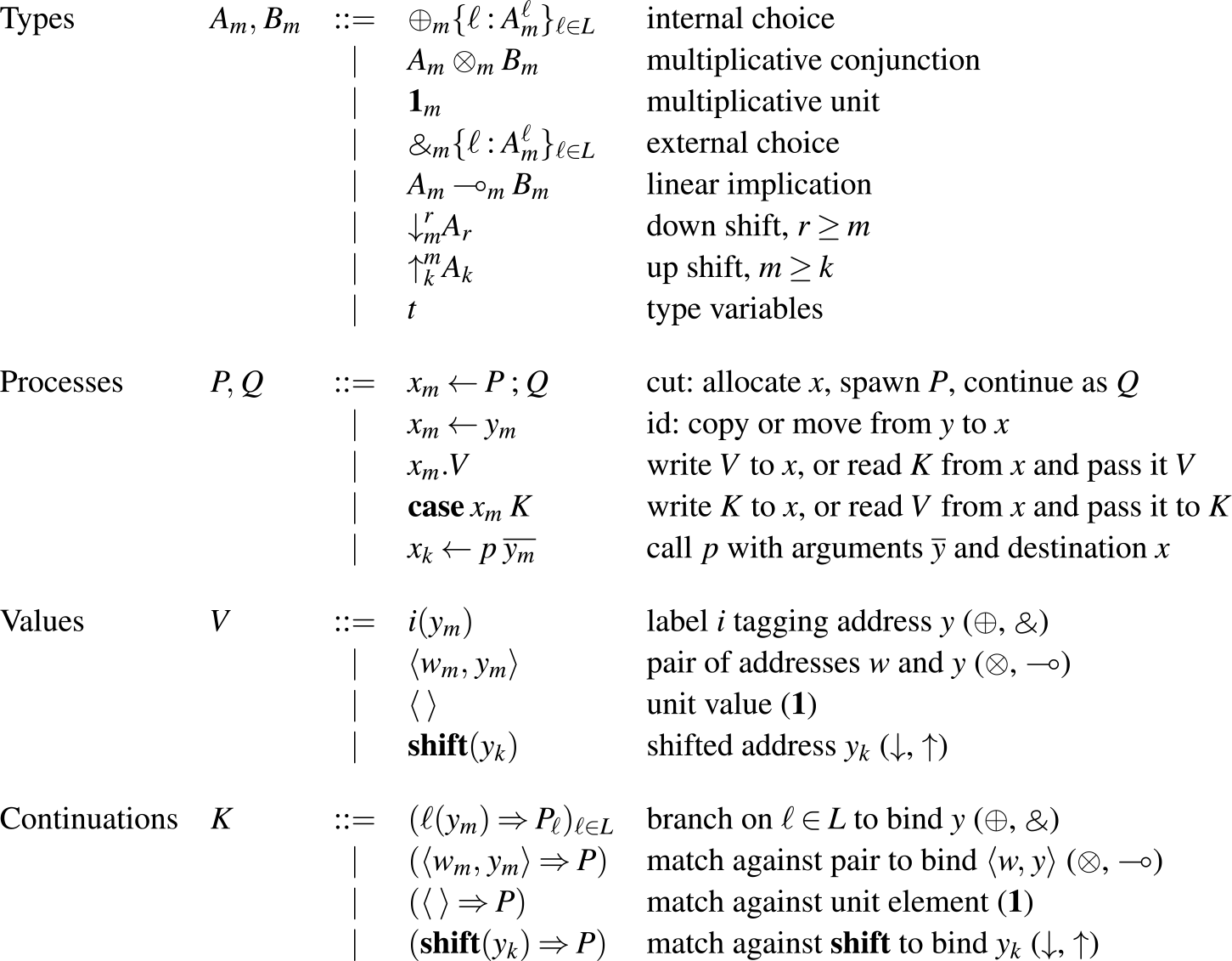
We can then give the following grammar for the propositions of (our presentation of) adjoint logic:
Here, $\multimap_m$
is implication,
$\multimap_m$
is implication, $\otimes_m$
is conjunction (more specifically, multiplicative conjunction if
$\otimes_m$
is conjunction (more specifically, multiplicative conjunction if $\sigma(m) = \{\}$
), and
$\sigma(m) = \{\}$
), and $\mathbf{1}_m$
is the multiplicative unit. The connectives
$\mathbf{1}_m$
is the multiplicative unit. The connectives $\oplus_{j \in J}$
and
$\oplus_{j \in J}$
and ![]() are additive disjunction and conjunction, respectively (often called internal and external choice in the session types literature), presented here in n-ary form because it is more natural for programming than the usual binary form.
are additive disjunction and conjunction, respectively (often called internal and external choice in the session types literature), presented here in n-ary form because it is more natural for programming than the usual binary form.
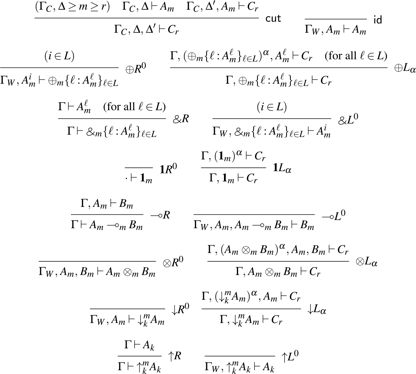
The rules for adjoint logic can be found in Figure 1, presented in a semi-axiomatic form DeYoung et al. (Reference DeYoung, Pfenning and Pruiksma2020), so some of the rules (indicated with a superscript 0) are axioms. In this formulation, contraction and weakening remain implicit.
Footnote 2
Handling contraction leads us to two versions of each of the $\oplus, \mathbf{1}, \otimes$
left rules, depending on whether the principal formula of the rule can be used again or not. The subscript
$\oplus, \mathbf{1}, \otimes$
left rules, depending on whether the principal formula of the rule can be used again or not. The subscript $\alpha$
on each of these rules may be either 0 or 1 and indicates whether the principal formula of the rule is preserved in the context. The
$\alpha$
on each of these rules may be either 0 or 1 and indicates whether the principal formula of the rule is preserved in the context. The $\alpha = 0$
version of each rule is the standard linear form, while the
$\alpha = 0$
version of each rule is the standard linear form, while the $\alpha = 1$
version, which requires that the mode m of the principal formula satisfies
$\alpha = 1$
version, which requires that the mode m of the principal formula satisfies $C \in \sigma(m)$
, keeps a copy of the principal formula. Note that if
$C \in \sigma(m)$
, keeps a copy of the principal formula. Note that if $C \in \sigma(m)$
, we are still allowed to use the
$C \in \sigma(m)$
, we are still allowed to use the $\alpha = 0$
version of the rule. Moreover, we write
$\alpha = 0$
version of the rule. Moreover, we write $\Gamma_C, \Gamma_W$
for contexts of variables all of which allow contraction or weakening, respectively. This allows us to freely drop weakenable variables when we reach initial rules, or to duplicate contractable variables to both parent and child when spawning a new process in the
$\Gamma_C, \Gamma_W$
for contexts of variables all of which allow contraction or weakening, respectively. This allows us to freely drop weakenable variables when we reach initial rules, or to duplicate contractable variables to both parent and child when spawning a new process in the $\textsf{cut}$
rule.
$\textsf{cut}$
rule.
Logical rules ( $\alpha \in \{0,1\}$
with
$\alpha \in \{0,1\}$
with $\alpha = 1$
permitted only if
$\alpha = 1$
permitted only if $C \in \sigma(m)$
).
$C \in \sigma(m)$
).
3 Seax: Types and syntax
The type system and language we present here, which we will use throughout this paper, begin with a Curry–Howard interpretation of adjoint logic, which we then leave behind by adding recursion, allowing a richer collection of programs.
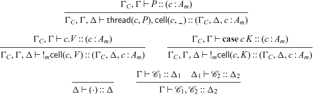
The types of Seax are the propositions of adjoint logic, augmented with general equirecursive types formed via mutually recursive type definitions in a global signature — most of the basic types are familiar as session types (Honda Reference Honda1993; Honda et al. Reference Honda, Vasconcelos and Kubo1998; Gay & Vasconcelos Reference Gay and Vasconcelos2010) (or as propositions of intuitionistic linear logic Girard & Lafont (Reference Girard and Lafont1987)), tagged with subscripts for modes. The grammar of types (as well as processes) can be found in Figure 2. Note that while our grammar includes mode subscripts on types, type constructors, and variables we will often omit them when they are clear from context.
Types and process expressions.
The typing judgment for processes has the form
 \begin{equation*} x_1:A^1_{m_1}, \ldots, x_n:A^n_{m_n} \vdash P :: (x : A_k)\end{equation*}
where P is a process expression and we require that each $m_i \geq k$
. Given such a judgment, we say that P provides or writes x, and uses or reads
$m_i \geq k$
. Given such a judgment, we say that P provides or writes x, and uses or reads $x_1, \ldots, x_n$
. We may often write a superscript on the variables to indicate whether they are being used for writing or reading. For instance, we would write
$x_1, \ldots, x_n$
. We may often write a superscript on the variables to indicate whether they are being used for writing or reading. For instance, we would write $x^{{\mathchoice{\textsf{W}}{\textsf{W}}{\scriptscriptstyle\textsf{W}}{\scriptscriptstyle\textsf{W}}}}$
in P to denote that P writes to x, and
$x^{{\mathchoice{\textsf{W}}{\textsf{W}}{\scriptscriptstyle\textsf{W}}{\scriptscriptstyle\textsf{W}}}}$
in P to denote that P writes to x, and $x_1^{{\mathchoice{\textsf{R}}{\textsf{R}}{\scriptscriptstyle\textsf{R}}{\scriptscriptstyle\textsf{R}}}}$
to denote that P reads from
$x_1^{{\mathchoice{\textsf{R}}{\textsf{R}}{\scriptscriptstyle\textsf{R}}{\scriptscriptstyle\textsf{R}}}}$
to denote that P reads from $x_1$
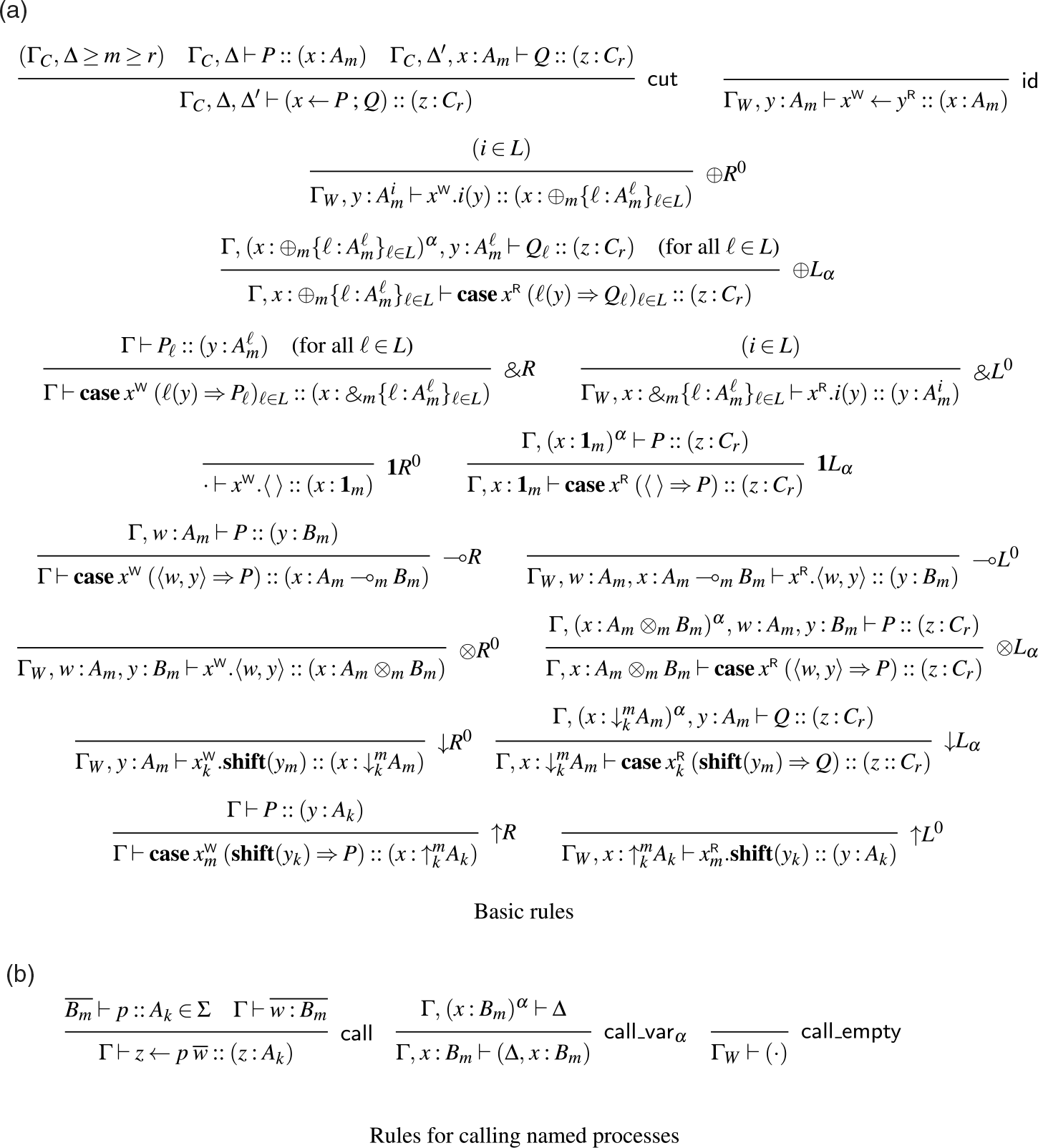
. While this information is not necessary for the semantics (and can in fact be inferred statically, and so is omitted from the formal semantics), it is convenient when writing down example processes for clarity, and so we will use it both in examples and in the typing rules, where it helps to clarify a key intuition of this system, which is that right rules write and left rules read. Not all reads and writes will be visible like this, however — we may call a process or invoke a stored continuation, and the resulting process may read or write (but since it is not obligated to, we do not mark these reads/writes at the callsite). The rules for this judgment can be found in Figure 3, and are just the logical rules from Figure 1, augmented with process terms and variables to label each assumption. We also include in this figure the rules for calling named processes, which make use of a fixed signature
$x_1$
. While this information is not necessary for the semantics (and can in fact be inferred statically, and so is omitted from the formal semantics), it is convenient when writing down example processes for clarity, and so we will use it both in examples and in the typing rules, where it helps to clarify a key intuition of this system, which is that right rules write and left rules read. Not all reads and writes will be visible like this, however — we may call a process or invoke a stored continuation, and the resulting process may read or write (but since it is not obligated to, we do not mark these reads/writes at the callsite). The rules for this judgment can be found in Figure 3, and are just the logical rules from Figure 1, augmented with process terms and variables to label each assumption. We also include in this figure the rules for calling named processes, which make use of a fixed signature $\Sigma$
for type and process definitions, as well as another judgment, which we explain later in this section.
$\Sigma$
for type and process definitions, as well as another judgment, which we explain later in this section.
Typing rules ( $\alpha \in \{0,1\}$
with
$\alpha \in \{0,1\}$
with $\alpha = 1$
permitted only if
$\alpha = 1$
permitted only if $C \in \sigma(m)$
).
$C \in \sigma(m)$
).
As usual, we require each of the $x_i$
and x to be distinct and allow silent renaming of bound variables
Footnote 3
in process expressions.
$x_i$
and x to be distinct and allow silent renaming of bound variables
Footnote 3
in process expressions.
Note that there is no explicit rule for (possibly recursively defined) type variables t, since they can be silently replaced by their definitions. Equality between types and type-checking can both easily be seen to be decidable using a combination of standard techniques for substructural-type systems (Cervesato et al. Reference Cervesato, Hodas and Pfenning2000) and subtyping for equirecursive session types, (Gay & Hole Reference Gay and Hole2005) which relies on a coinductive interpretation of the types, but not on their linearity, and so can be adapted to the adjoint setting. Some experience with a closely related algorithm (Das & Pfenning Reference Das and Pfenning2020) for type equality and type checking suggests that this is practical.
We now go on to briefly examine the terms and loosely describe their meanings from the perspective of a shared-memory semantics. We will make this more precise in Sections 4 and 5, where we develop the dynamics of such a shared-memory semantics.
Both the grammar and the typing rules show that we have five primary constructs for processes, which then break down further into specific cases.
The first two process constructs are type-agnostic. The $\textsf{cut}$
rule, with term
$\textsf{cut}$
rule, with term $x \leftarrow P \mathrel{;} Q$
, allocates a new memory cell x, spawns a new process P which may write to x, and continues as Q which may read from x. The new cell x thus serves as the point of communication between the new process P and the continuing Q. The
$x \leftarrow P \mathrel{;} Q$
, allocates a new memory cell x, spawns a new process P which may write to x, and continues as Q which may read from x. The new cell x thus serves as the point of communication between the new process P and the continuing Q. The $\textsf{id}$
rule, with term
$\textsf{id}$
rule, with term $x_m \leftarrow y_m$
, copies the contents of cell
$x_m \leftarrow y_m$
, copies the contents of cell $y_m$
into cell
$y_m$
into cell $x_m$
. If
$x_m$
. If $C \notin \sigma(m)$
, we can think of this instead as moving the contents of cell
$C \notin \sigma(m)$
, we can think of this instead as moving the contents of cell $y_m$
into cell
$y_m$
into cell $x_m$
and freeing
$x_m$
and freeing $y_m$
.
$y_m$
.
The next two constructs, $x.V$
and
$x.V$
and $\mathbf{case}\, x\, K$
, come in pairs that perform communication, one pair for each type. A process of one of these forms will either write to or read from x, depending on whether the variable is in the succedent (write) or antecedent (read).
$\mathbf{case}\, x\, K$
, come in pairs that perform communication, one pair for each type. A process of one of these forms will either write to or read from x, depending on whether the variable is in the succedent (write) or antecedent (read).
A write is straightforward and stores either the value V or the continuation K into the cell x, while a read pulls a continuation K’ or a value V’ from the cell, and combines either K’ and V (in the case of $x.V$
) or K and V’ (
$x.V$
) or K and V’ ( $\mathbf{case}\, x\, K$
). The symmetry of this, in which continuations and values are both eligible to be written to memory and read from memory, comes from the duality between
$\mathbf{case}\, x\, K$
). The symmetry of this, in which continuations and values are both eligible to be written to memory and read from memory, comes from the duality between $\oplus$
and
$\oplus$
and ![]() , between
, between $\otimes$
and
$\otimes$
and $\multimap$
, and between
$\multimap$
, and between ${\downarrow}$
and
${\downarrow}$
and ${\uparrow}$
. We see this in the typing rules, where, for instance,
${\uparrow}$
. We see this in the typing rules, where, for instance, $\oplus R^0$
and
$\oplus R^0$
and ![]() have the same process term, swapping only the roles of each variable between read and write. However, the values do have different meaning depending on whether they are being used to read or to write. In the case of
have the same process term, swapping only the roles of each variable between read and write. However, the values do have different meaning depending on whether they are being used to read or to write. In the case of $x^{{\mathchoice{\textsf{W}}{\textsf{W}}{\scriptscriptstyle\textsf{W}}{\scriptscriptstyle\textsf{W}}}}.\langle y, z \rangle$
, for instance, we are writing a pair of addresses
$x^{{\mathchoice{\textsf{W}}{\textsf{W}}{\scriptscriptstyle\textsf{W}}{\scriptscriptstyle\textsf{W}}}}.\langle y, z \rangle$
, for instance, we are writing a pair of addresses $\langle y, z \rangle$
to address x (though this does not guarantee that the cells at addresses y or z have been filled in). A future reader K of x will see addresses y and z, and is entitled to read from them. By contrast,
$\langle y, z \rangle$
to address x (though this does not guarantee that the cells at addresses y or z have been filled in). A future reader K of x will see addresses y and z, and is entitled to read from them. By contrast, $w^{{\mathchoice{\textsf{R}}{\textsf{R}}{\scriptscriptstyle\textsf{R}}{\scriptscriptstyle\textsf{R}}}}.\langle u, v \rangle$
reads a continuation K out of the cell at address w and passes it the pair of addresses
$w^{{\mathchoice{\textsf{R}}{\textsf{R}}{\scriptscriptstyle\textsf{R}}{\scriptscriptstyle\textsf{R}}}}.\langle u, v \rangle$
reads a continuation K out of the cell at address w and passes it the pair of addresses $\langle u, v \rangle$
. Unlike in the previous case, the continuation K is entitled to read from u, but to write to v.
Footnote 4
We can think of u as the argument being passed in to K, and v as the destination where K should store its result, as in the destination-passing style (Wadler Reference Wadler1984; Larus Reference Larus1989; Cervesato et al. Reference Cervesato, Pfenning, Walker and Watkins2002; Simmons Reference Simmons2012) of semantics for functional languages.
$\langle u, v \rangle$
. Unlike in the previous case, the continuation K is entitled to read from u, but to write to v.
Footnote 4
We can think of u as the argument being passed in to K, and v as the destination where K should store its result, as in the destination-passing style (Wadler Reference Wadler1984; Larus Reference Larus1989; Cervesato et al. Reference Cervesato, Pfenning, Walker and Watkins2002; Simmons Reference Simmons2012) of semantics for functional languages.
As cells may contain either values V or continuations K, it will be useful to have a way to refer to this class of expression:
 \begin{equation*} \mbox{Cell data} \qquad D ::= V \mid K \end{equation*}
The final construct allows for calling named processes, which we use for recursion. As is customary in session types, we use equirecursive types, collected in a signature $\Sigma$
in which we also collect recursive process definitions and their types. For each type definition
$\Sigma$
in which we also collect recursive process definitions and their types. For each type definition $t = A$
, the type A must be contractive so that we can treat types equirecursively with a straightforward coinductive definition and an efficient algorithm for type equality (Gay & Hole Reference Gay and Hole2005).
$t = A$
, the type A must be contractive so that we can treat types equirecursively with a straightforward coinductive definition and an efficient algorithm for type equality (Gay & Hole Reference Gay and Hole2005).
A named process p is declared as $B^1_{m_1}, \ldots, B^n_{m_n} \vdash p :: A_k$
which means it requires arguments of types
$B^1_{m_1}, \ldots, B^n_{m_n} \vdash p :: A_k$
which means it requires arguments of types $B^i_{m_i}$
(in that order) and provides a result of type
$B^i_{m_i}$
(in that order) and provides a result of type $A_k$
. For ease of readability, we may sometimes write in variable names as well, but they are actually only needed for the corresponding definitions
$A_k$
. For ease of readability, we may sometimes write in variable names as well, but they are actually only needed for the corresponding definitions $x \leftarrow p \; y_1, \ldots, y_n = P$
.
$x \leftarrow p \; y_1, \ldots, y_n = P$
.
We can then formally define signatures as follows, allowing definitions of types, declarations of processes, and definitions of processes:
 \begin{equation*} \begin{array}{llcl} \mbox{Signatures} & \Sigma & ::= & \cdot \mid \Sigma, t = A \mid \Sigma, \overline{B_m} \vdash p :: A_k \mid \Sigma, x \leftarrow p \; \overline{y} = P \end{array}\end{equation*}
For valid signatures, we require that each declaration $\overline{B_m} \vdash p :: A_k$
has a corresponding definition
$\overline{B_m} \vdash p :: A_k$
has a corresponding definition $x \leftarrow p \; \overline{y} = P$
with
$x \leftarrow p \; \overline{y} = P$
with $\overline{y : B_m} \vdash P :: (x : A_k)$
. This means that all type and process definitions can be mutually recursive.
$\overline{y : B_m} \vdash P :: (x : A_k)$
. This means that all type and process definitions can be mutually recursive.
In the remainder of this paper, we assume that we have a fixed valid signature $\Sigma$
, so we annotate neither the typing judgment nor the computation rules with an explicit signature, other than in the
$\Sigma$
, so we annotate neither the typing judgment nor the computation rules with an explicit signature, other than in the $\textsf{call}$
rule, where we extract a process definition from
$\textsf{call}$
rule, where we extract a process definition from $\Sigma$
.
$\Sigma$
.
Operationally, a call $z \leftarrow p \; \overline{w}$
expands to its definition with a substitution
$z \leftarrow p \; \overline{w}$
expands to its definition with a substitution $[\overline{w}/\overline{y}, z/x]P$
, replacing variables by addresses. In order to type a call, therefore, we need to ensure that this substitution is valid. The substitution of z for x is always valid, and so we check the remainder of the substitution with the rules
$[\overline{w}/\overline{y}, z/x]P$
, replacing variables by addresses. In order to type a call, therefore, we need to ensure that this substitution is valid. The substitution of z for x is always valid, and so we check the remainder of the substitution with the rules $\textsf{call_var}_\alpha$
and
$\textsf{call_var}_\alpha$
and $\textsf{call_empty}$
, defining a judgment
$\textsf{call_empty}$
, defining a judgment $\Gamma \vdash \overline{w : B_m}$
which verifies that
$\Gamma \vdash \overline{w : B_m}$
which verifies that $\Gamma$
can provide the arguments
$\Gamma$
can provide the arguments $\overline{w : B_m}$
to the process.
$\overline{w : B_m}$
to the process.
4 Concurrent semantics
We will now present a concurrent shared-memory semantics for Seax, using multiset rewriting rules (Cervesato & Scedrov Reference Cervesato and Scedrov2009). The state of a running program is a multiset of semantic objects, which we refer to as a process configuration. We have three distinct types of semantic objects, each of which tracks the address it provides, in order to link it with users of that address:
-
1. $\textsf{thread}(c_m, P)$
: thread executing P with destination
$c_m$
$\textsf{thread}(c_m, P)$
: thread executing P with destination
$c_m$
-
2.
$\textsf{cell}(c_m, \_)$
: cell
$c_m$
that has been allocated, but not yet written -
3.
${!}_m \textsf{cell}(c_m, D)$
: cell
$c_m$
containing data D


Here, we prefix a semantic object with ${!}_m$
to indicate that it is persistent when
${!}_m$
to indicate that it is persistent when $C \in \sigma(m)$
, and ephemeral otherwise. Note that empty cells are always ephemeral, so that we can modify them by writing to them, while filled cells may be persistent, as each cell has exactly one writer, which will terminate on writing. We maintain the invariant that in a configuration either
$C \in \sigma(m)$
, and ephemeral otherwise. Note that empty cells are always ephemeral, so that we can modify them by writing to them, while filled cells may be persistent, as each cell has exactly one writer, which will terminate on writing. We maintain the invariant that in a configuration either $\textsf{thread}(c_m, P)$
appears together with
$\textsf{thread}(c_m, P)$
appears together with $\textsf{cell}(c_m, \_)$
, or we have just
$\textsf{cell}(c_m, \_)$
, or we have just ${!}_m \textsf{cell}(c_m, D)$
, as well as that if two semantic objects provide the same address
${!}_m \textsf{cell}(c_m, D)$
, as well as that if two semantic objects provide the same address $c_m$
, then they are exactly a
$c_m$
, then they are exactly a $\textsf{thread}(c_m, P)$
,
$\textsf{thread}(c_m, P)$
, $\textsf{cell}(c_m, \_)$
pair. While this invariant can be made slightly cleaner by removing the
$\textsf{cell}(c_m, \_)$
pair. While this invariant can be made slightly cleaner by removing the $\textsf{cell}(c_m, \_)$
objects, this leads to an interpretation where cells are allocated lazily just before they are written. While this has some advantages, it is unclear how to inform the thread which will eventually read from the new cell where said cell can be found, and so, in the interest of having a realistically implementable semantics, we just allocate an empty cell on spawning a new thread, allowing the parent thread to see the location of that cell.
$\textsf{cell}(c_m, \_)$
objects, this leads to an interpretation where cells are allocated lazily just before they are written. While this has some advantages, it is unclear how to inform the thread which will eventually read from the new cell where said cell can be found, and so, in the interest of having a realistically implementable semantics, we just allocate an empty cell on spawning a new thread, allowing the parent thread to see the location of that cell.
We can then define configurations with the following grammar (and the additional constraint of our invariant):
 \begin{equation*} \begin{array}{llcl} \mbox{Configurations} & \mathcal{C} & ::= & \cdot \mid \textsf{thread}(c_m, P), \textsf{cell}(c_m, \_) \mid {!}_m \textsf{cell}(c_m, D) \mid \mathcal{C}_1, \mathcal{C}_2 \end{array}\end{equation*}
We think of the join $\mathcal{C}_1, \mathcal{C}_2$
of two configurations as a commutative and associative operation so that this grammar defines a multiset rather than a list or tree.
$\mathcal{C}_1, \mathcal{C}_2$
of two configurations as a commutative and associative operation so that this grammar defines a multiset rather than a list or tree.
A multiset rewriting rule takes the collection of objects on the left-hand side of the rule, consumes them (if they are ephemeral), and then adds in the objects on the right-hand side of the rule. Rules may be applied to any subconfiguration, leaving the remainder of the configuration unchanged. This yields a naturally nondeterministic semantics, but we will see that the semantics are nonetheless confluent (Theroem 3). Additionally, while our configurations are not ordered, we will adopt the convention that the writer of an address appears to the left of any readers of that address.
Our semantic rules are based on a few key ideas:
-
1. Variables represent addresses in shared memory.
-
2. Cut/spawn is the only way to allocate a new cell.
-
3. Identity/forward will move or copy data between cells.
-
4. A process
$\textsf{thread}(c, P)$
will (eventually) write to the cell at address c and then terminate. -
5. A process
$\textsf{thread}(d, Q)$
that is trying to read from
$c \neq d$
will wait until the cell with address c is available (i.e. its contents is no longer
$\_$
), perform the read, and then continue.


The counterintuitive part of this interpretation (when using a message-passing semantics as a point of reference) is that a process providing ![]() does not read a value from shared memory. Instead, it writes a continuation to memory and terminates. Conversely, a client of such a channel does not write a value to shared memory. Instead, it continues by jumping to the continuation. This ability to write continuations to memory is a major feature distinguishing this from a message-passing semantics where potentially large closures would have to be captured, serialized, and deserialized, the cost of which is difficult to control (Miller et al. Reference Miller, Haller, MÜller and Boullier2016).
does not read a value from shared memory. Instead, it writes a continuation to memory and terminates. Conversely, a client of such a channel does not write a value to shared memory. Instead, it continues by jumping to the continuation. This ability to write continuations to memory is a major feature distinguishing this from a message-passing semantics where potentially large closures would have to be captured, serialized, and deserialized, the cost of which is difficult to control (Miller et al. Reference Miller, Haller, MÜller and Boullier2016).
The final piece that we need to present the semantics is a key operation, namely that of passing a value V to a continuation K to get a new process P. This operation is defined as follows:
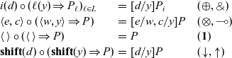
When any of these reductions is applied, either the value or the continuation has been read from a cell while the other is a part of the executing process. With this notation, we can give a concise set of rules for the concurrent dynamics. We present these rules in Figure 4.
Concurrent dynamic rules
(All addresses with distinct names [e.g. $c_m$
and
$c_m$
and $d_m$
] are different).
$d_m$
] are different).
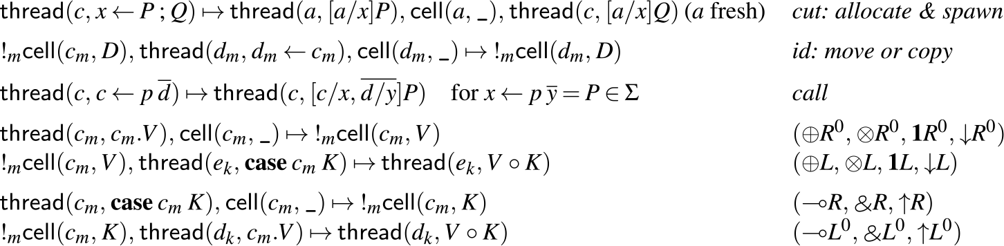
These rules match well with our intuitions from before. In the cut rule, we allocate a new empty cell a, spawn a new thread to execute P, and continue executing Q, just as we described informally in Section 3. Similarly, in the id rule, we either move or copy (depending on whether $C \in \sigma(m)$
) the contents of cell c into cell d and terminate. The rules that write values to cells are exactly the right rules for positive types (
$C \in \sigma(m)$
) the contents of cell c into cell d and terminate. The rules that write values to cells are exactly the right rules for positive types ( $\oplus, \otimes, \mathbf{1}, {\downarrow}$
), while the right rules for negative types (
$\oplus, \otimes, \mathbf{1}, {\downarrow}$
), while the right rules for negative types (![]() ) write continuations to cells instead. Dually, to read from a cell of positive type, we must have a continuation to pass the stored value to, while to read from a cell of negative type, we need a value to pass to the stored continuation.
) write continuations to cells instead. Dually, to read from a cell of positive type, we must have a continuation to pass the stored value to, while to read from a cell of negative type, we need a value to pass to the stored continuation.
4.1 Results
We have standard results for this system — a form of progress, of preservation, and a confluence result. To discuss progress and preservation, we must first extend our notion of typing for process terms to configurations. Configurations are typed with the judgment $\Gamma \vdash \mathcal{C} :: \Delta$
which means that configuration
$\Gamma \vdash \mathcal{C} :: \Delta$
which means that configuration $\mathcal{C}$
may read from the addresses in
$\mathcal{C}$
may read from the addresses in $\Gamma$
and write to the addresses in
$\Gamma$
and write to the addresses in $\Delta$
. We can then give the following set of rules for typing configurations, which make use of the typing judgment
$\Delta$
. We can then give the following set of rules for typing configurations, which make use of the typing judgment $\Gamma \vdash P :: (c : A_m)$
for process terms in the base cases. Recall that we use
$\Gamma \vdash P :: (c : A_m)$
for process terms in the base cases. Recall that we use $\Gamma_C$
to denote a context in which all propositions are contractible, and which can therefore be freely duplicated.
$\Gamma_C$
to denote a context in which all propositions are contractible, and which can therefore be freely duplicated.
Note that our invariants on configurations mean that there is no need to separately type the objects $\textsf{thread}(c, P)$
and
$\textsf{thread}(c, P)$
and $\textsf{cell}(c, \_)$
, as they can only occur together. Additionally, while our configurations are multisets, and therefore not inherently ordered, observe that the typing derivation for a configuration induces an order on the configuration, something which is quite useful in proving progress.
Footnote 5
$\textsf{cell}(c, \_)$
, as they can only occur together. Additionally, while our configurations are multisets, and therefore not inherently ordered, observe that the typing derivation for a configuration induces an order on the configuration, something which is quite useful in proving progress.
Footnote 5
Our preservation theorem differs slightly from the standard, in that it allows the collection of typed channels $\Delta$
offered by a configuration
$\Delta$
offered by a configuration $\mathcal{C}$
to grow after a step, as steps may introduce new persistent memory cells. Note that the
$\mathcal{C}$
to grow after a step, as steps may introduce new persistent memory cells. Note that the $\Delta$
cannot shrink, despite the fact that affine or linear cells may be deallocated after read. This is because a linear cell that is read from never appeared in
$\Delta$
cannot shrink, despite the fact that affine or linear cells may be deallocated after read. This is because a linear cell that is read from never appeared in $\Delta$
in the first place — the process that reads it also consumes it in the typing derivation. Likewise, an affine cell that is read from will not appear in
$\Delta$
in the first place — the process that reads it also consumes it in the typing derivation. Likewise, an affine cell that is read from will not appear in $\Delta$
, while an affine cell with no reader appears in
$\Delta$
, while an affine cell with no reader appears in $\Delta$
(but of course, since it has no reader, it will not be deallocated).
$\Delta$
(but of course, since it has no reader, it will not be deallocated).
Theorem 1 (Type Preservation) If $\Gamma \vdash \mathcal{C} :: \Delta$
and
$\Gamma \vdash \mathcal{C} :: \Delta$
and $\mathcal{C} \mapsto \mathcal{C}'$
then
$\mathcal{C} \mapsto \mathcal{C}'$
then $\Gamma \vdash \mathcal{C}' :: \Delta'$
for some
$\Gamma \vdash \mathcal{C}' :: \Delta'$
for some $\Delta' \supseteq \Delta$
.
$\Delta' \supseteq \Delta$
.
Proof. By cases on the transition relation for configurations, applying repeated inversions to the typing judgment on $\mathcal{C}$
to obtain the necessary information to assemble a typing derivation for
$\mathcal{C}$
to obtain the necessary information to assemble a typing derivation for $\mathcal{C}'$
. This requires some straightforward lemmas expressing that non-interfering processes and cells can be exchanged in a typing derivation.
$\mathcal{C}'$
. This requires some straightforward lemmas expressing that non-interfering processes and cells can be exchanged in a typing derivation. $\square$
Progress is entirely standard, with configurations comprised entirely of filled cells taking the role that values play in a functional language.
Theorem 2 (Progress) If $\cdot \vdash \mathcal{C} :: \Delta$
then either
$\cdot \vdash \mathcal{C} :: \Delta$
then either $\mathcal{C} \mapsto \mathcal{C}'$
for some
$\mathcal{C} \mapsto \mathcal{C}'$
for some $\mathcal{C}'$
, or for every channel
$\mathcal{C}'$
, or for every channel $c_m : A_m \in \Delta$
there is an object
$c_m : A_m \in \Delta$
there is an object ${!}_m \textsf{cell}(c_m,D) \in \mathcal{C}$
.
${!}_m \textsf{cell}(c_m,D) \in \mathcal{C}$
.
Proof. We first re-associate all applications of the typing rule for joining configurations to the left. Then we perform an induction over the structure of the resulting derivation, distinguishing cases for the rightmost cell or thread and potentially applying the induction hypothesis on the configuration to its left. This structure, together with inversion on the typing of the cell or thread yields the theorem. $\square$
In addition to these essential properties, we also have a confluence result, for which we need to define a weak notion of equivalence on configurations. We say $\mathcal{C}_1 \sim \mathcal{C}_2$
if there is a renaming
$\mathcal{C}_1 \sim \mathcal{C}_2$
if there is a renaming $\rho$
of addresses such that
$\rho$
of addresses such that $\rho\mathcal{C}_1 = \mathcal{C}_2$
. We can then establish the following version of the diamond property:
$\rho\mathcal{C}_1 = \mathcal{C}_2$
. We can then establish the following version of the diamond property:
Theorem 3 (Diamond Property) $\Delta \vdash \mathcal{C} :: \Gamma$
. If
$\Delta \vdash \mathcal{C} :: \Gamma$
. If $\mathcal{C} \mapsto \mathcal{C}_1$
and
$\mathcal{C} \mapsto \mathcal{C}_1$
and $\mathcal{C} \mapsto \mathcal{C}_2$
such that
$\mathcal{C} \mapsto \mathcal{C}_2$
such that $\mathcal{C}_1 \not\sim \mathcal{C}_2$
. Then there exist
$\mathcal{C}_1 \not\sim \mathcal{C}_2$
. Then there exist $\mathcal{C}_1'$
and
$\mathcal{C}_1'$
and $\mathcal{C}_2'$
such that
$\mathcal{C}_2'$
such that $\mathcal{C}_1 \mapsto \mathcal{C}_1'$
and
$\mathcal{C}_1 \mapsto \mathcal{C}_1'$
and $\mathcal{C}_2 \mapsto \mathcal{C}_2'$
with
$\mathcal{C}_2 \mapsto \mathcal{C}_2'$
with $\mathcal{C}_1' \sim \mathcal{C}_2'$
.
$\mathcal{C}_1' \sim \mathcal{C}_2'$
.
Proof. The proof is straightforward by cases. There are no critical pairs involving ephemeral (that is, non-persistent) objects in the left-hand sides of transition rules. $\square$
4.2 Examples
We present here a few examples of concurrent programs, illustrating various aspects of our language.
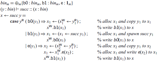
4.2.1 Example: Binary Numbers.
As a first simple example we consider binary numbers, defined as a type bin at mode m. The structural properties of mode m are arbitrary for our examples. For concreteness, assume that m is linear, that is, $\sigma(m) = \{\,\}$
.
$\sigma(m) = \{\,\}$
.
 \begin{equation*} {bin}_m = {\oplus}_m\{\textsf{b0} : {bin}_m, \textsf{b1} : {bin}_m, \textsf{e} : \mathbf{1}_m\}\end{equation*}
Unless multiple modes are involved, we will henceforth omit the mode m. As an example, the number $6 = (110)_2$
would be represented by a sequence of labels
$6 = (110)_2$
would be represented by a sequence of labels $\textsf{e}, \textsf{b1}, \textsf{b1}, \textsf{b0}$
, chained together in a linked list. The first cell in the list would contain the bit
$\textsf{e}, \textsf{b1}, \textsf{b1}, \textsf{b0}$
, chained together in a linked list. The first cell in the list would contain the bit $\textsf{b0}$
. It has some address
$\textsf{b0}$
. It has some address $c_0$
, and also contains an address
$c_0$
, and also contains an address $c_1$
pointing to the next cell in the list. Writing out the whole sequence as a configuration we have
$c_1$
pointing to the next cell in the list. Writing out the whole sequence as a configuration we have
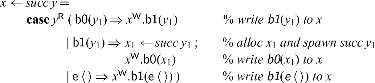
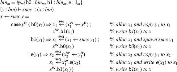
4.2.2 Example: Computing with Binary Numbers.
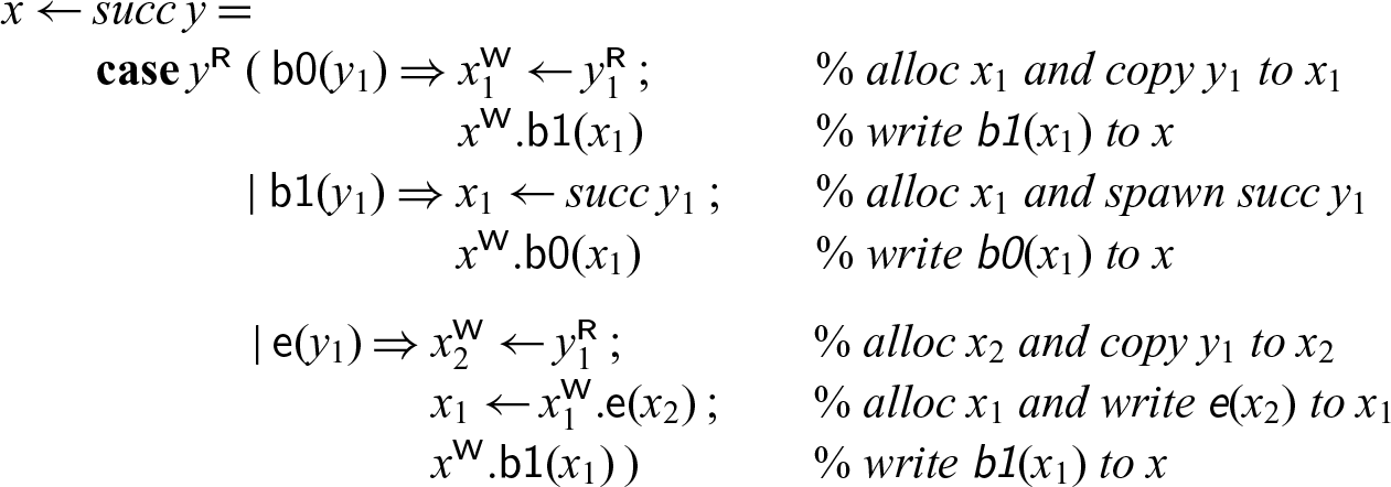
We implement a recursive process succ that reads the bits of a binary number n starting at address y and writes the bits for the binary number $n+1$
starting at x. This process may block until the input cell (referenced as y) has been written to; the output cells are allocated one by one as needed. Since we assumed the mode m is linear, the cells read by the succ process from will be deallocated.
$n+1$
starting at x. This process may block until the input cell (referenced as y) has been written to; the output cells are allocated one by one as needed. Since we assumed the mode m is linear, the cells read by the succ process from will be deallocated.
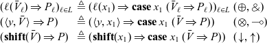
In this example and others, we find certain repeating patterns. Abbreviating these makes the code easier to read and also more compact to write. As a first simplification, we can use the following shortcuts:
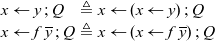 \begin{equation*} \begin{array}{lcll} x \leftarrow y \mathrel{;} Q & \triangleq & x\leftarrow (x \leftarrow y) \mathrel{;} Q \\ x \leftarrow f \; \overline{y} \mathrel{;} Q & \triangleq & x \leftarrow (x \leftarrow f \; \overline{y}) \mathrel{;} Q \end{array}\end{equation*}
With these, the code for successor becomes
The second pattern we notice are sequences of allocations followed by immediate (single) uses of the new address. We can collapse these by a kind of specialized substitution. We describe the inverse, namely how the abbreviated notation is elaborated into the language primitives.
 \begin{equation*} \begin{array}{llcl} \mbox{Value Sequence} & \bar{V} & ::= & i(\bar{V}) \mid (y,\bar{V}) \mid \mathbf{shift}(\bar{V}) \mid V \end{array}\end{equation*}
At positive types ( ${\oplus},{\otimes},{\mathbf{1}},{{\downarrow}}$
), which write to the variable x with
${\oplus},{\otimes},{\mathbf{1}},{{\downarrow}}$
), which write to the variable x with $x.\bar{V}$
, we define:
$x.\bar{V}$
, we define:
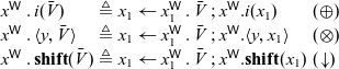 \begin{equation*} \begin{array}{lcll} x^{{\mathchoice{\textsf{W}}{\textsf{W}}{\scriptscriptstyle\textsf{W}}{\scriptscriptstyle\textsf{W}}}}\mathrel{.} i(\bar{V}) & \triangleq & x_1 \leftarrow x_1^{{\mathchoice{\textsf{W}}{\textsf{W}}{\scriptscriptstyle\textsf{W}}{\scriptscriptstyle\textsf{W}}}}\mathrel{.} \bar{V} \mathrel{;} x^{{\mathchoice{\textsf{W}}{\textsf{W}}{\scriptscriptstyle\textsf{W}}{\scriptscriptstyle\textsf{W}}}}.i(x_1) & (\oplus) \\ x^{{\mathchoice{\textsf{W}}{\textsf{W}}{\scriptscriptstyle\textsf{W}}{\scriptscriptstyle\textsf{W}}}}\mathrel{.} \langle y,\bar{V}\rangle & \triangleq & x_1 \leftarrow x_1^{{\mathchoice{\textsf{W}}{\textsf{W}}{\scriptscriptstyle\textsf{W}}{\scriptscriptstyle\textsf{W}}}}\mathrel{.} \bar{V} \mathrel{;} x^{{\mathchoice{\textsf{W}}{\textsf{W}}{\scriptscriptstyle\textsf{W}}{\scriptscriptstyle\textsf{W}}}}.\langle y,x_1\rangle & (\otimes) \\ x^{{\mathchoice{\textsf{W}}{\textsf{W}}{\scriptscriptstyle\textsf{W}}{\scriptscriptstyle\textsf{W}}}}\mathrel{.} \mathbf{shift}(\bar{V}) & \triangleq & x_1 \leftarrow x_1^{{\mathchoice{\textsf{W}}{\textsf{W}}{\scriptscriptstyle\textsf{W}}{\scriptscriptstyle\textsf{W}}}}\mathrel{.} \bar{V} \mathrel{;} x^{{\mathchoice{\textsf{W}}{\textsf{W}}{\scriptscriptstyle\textsf{W}}{\scriptscriptstyle\textsf{W}}}}.\mathbf{shift}(x_1) & ({\downarrow}) \\ \end{array}\end{equation*}
In each case, and similar definitions below, $x_1$
is a fresh variable. Using these abbreviations in our example, we can shorten it further.
$x_1$
is a fresh variable. Using these abbreviations in our example, we can shorten it further.
For negative types (![]() ) the expansion is symmetric, swapping the left- and right-hand sides of the cut. This is because these constructs read a continuation from memory at x and pass it a value.
) the expansion is symmetric, swapping the left- and right-hand sides of the cut. This is because these constructs read a continuation from memory at x and pass it a value.
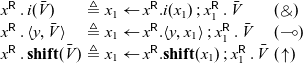
Similarly, we can decompose a continuation matching against a value sequence $(\bar{V} \Rightarrow P)$
. For simplicity, we assume here that the labels for each branch of a pattern match for internal (
$(\bar{V} \Rightarrow P)$
. For simplicity, we assume here that the labels for each branch of a pattern match for internal ( $\oplus$
) or external (
$\oplus$
) or external (![]() ) choice are distinct; a generalization to nested patterns is conceptually straightforward but syntactically somewhat complex so we do not specify it formally.
) choice are distinct; a generalization to nested patterns is conceptually straightforward but syntactically somewhat complex so we do not specify it formally.
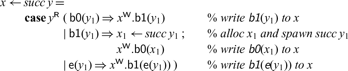
For example, we can rewrite the successor program one more time to express that $y_1$
in the last case must actually contain the unit element
$y_1$
in the last case must actually contain the unit element $\langle\,\rangle$
and match against it as well as construct it on the right-hand side.
$\langle\,\rangle$
and match against it as well as construct it on the right-hand side.
We have to remember, however, that intermediate matches and allocations still take place and the last two programs are not equivalent in case the process with destination y’ does not terminate.
To implement plus2 we can just compose succ with itself.

In our concurrent semantics, the two successor processes form a concurrently executing pipeline — the first reads the initial number from memory, bit by bit, and then writes a new number (again, bit by bit) to memory for the second successor process to read.
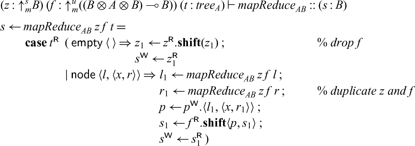
4.2.3 Example: MapReduce.
As a second example we consider mapReduce applied to a tree. We have a neutral element z (which stands in for every leaf) and a process f to be applied at every node to reduce the whole tree to a single value. This exhibits a high degree of parallelism, since the operations on the left and right subtree can be done independently. We abstract over the type of element A and the result B at the meta-level, so that $\textsf{tree}_A$
is a family of types, and
$\textsf{tree}_A$
is a family of types, and ${mapReduce}_{AB}$
is a family of processes, indexed by A and B.
${mapReduce}_{AB}$
is a family of processes, indexed by A and B.
 \begin{equation*}{tree}_A = {\oplus}_m\{\textsf{empty} : \mathbf{1}, \textsf{node} : {tree}_A \otimes A \otimes {tree}_A\}\end{equation*}
Since mapReduce applies reduction at every node in the tree, it is linear in the tree. On the other hand, the neutral element z is used for every leaf, and the associative operation f for every node, so z requires at least contraction (there must be at least one leaf) and f both weakening and contraction (there may be arbitrarily many nodes). Therefore, we use three modes: the linear mode m for the tree and the result of mapReduce, a strict mode s for the neutral element z, and an unrestricted mode u for the operation applied at each node.
4.2.4 Example: λ-Calculus.
As a third example, we show an encoding of the $\lambda$
-calculus using higher order abstract syntax and parallel evaluation. We specify, at an arbitrary mode m:
$\lambda$
-calculus using higher order abstract syntax and parallel evaluation. We specify, at an arbitrary mode m:
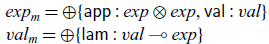 \begin{equation*} {exp}_m = \oplus\{\textsf{app} : {exp} \otimes {exp}, \textsf{val} : {val}\} \\ {val}_m = \oplus\{\textsf{lam} : {val} \multimap {exp}\}\end{equation*}
An interesting property of this representation is that if we pick m to be linear, we obtain the linear $\lambda$
-calculus (Lincoln & Mitchell Reference Lincoln and Mitchell1992), if we pick m to be strict (
$\lambda$
-calculus (Lincoln & Mitchell Reference Lincoln and Mitchell1992), if we pick m to be strict ( $\sigma(m) = \{C\}$
) we obtain Church and Rosser’s original
$\sigma(m) = \{C\}$
) we obtain Church and Rosser’s original $\lambda I$
calculus (Church & Rosser Reference Church and Rosser1936), and if we set
$\lambda I$
calculus (Church & Rosser Reference Church and Rosser1936), and if we set $\sigma(m) = \{W,C\}$
we obtain the usual (intuitionistic)
$\sigma(m) = \{W,C\}$
we obtain the usual (intuitionistic) $\lambda$
-calculus. Evaluation (that is, parallel reduction to a weak head-normal form) is specified by the following process, no matter which version of the
$\lambda$
-calculus. Evaluation (that is, parallel reduction to a weak head-normal form) is specified by the following process, no matter which version of the $\lambda$
-calculus we consider.
$\lambda$
-calculus we consider.
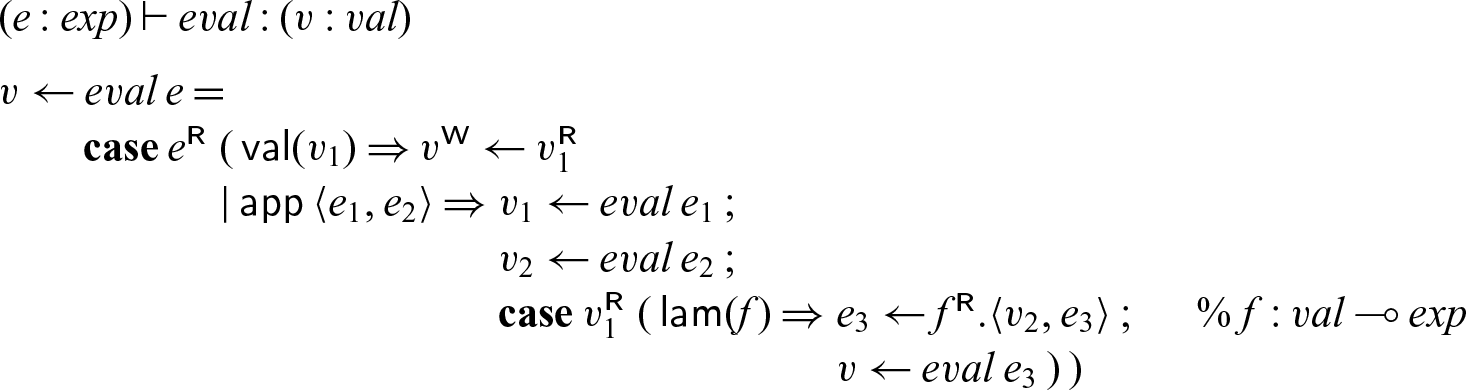
In this code, $v_2$
acts like a future: we spawn the evaluation of
$v_2$
acts like a future: we spawn the evaluation of $e_2$
with the promise to place the result in
$e_2$
with the promise to place the result in $v_2$
. In our dynamics, we allocate a new cell for
$v_2$
. In our dynamics, we allocate a new cell for $v_2$
, as yet unfilled. When we pass
$v_2$
, as yet unfilled. When we pass $v_2$
to f in
$v_2$
to f in $f.\langle v_2,e_3\rangle$
the process
$f.\langle v_2,e_3\rangle$
the process ${eval}\; e_2$
may still be computing, and we will not block until we eventually try to read from
${eval}\; e_2$
may still be computing, and we will not block until we eventually try to read from $v_2$
(which may or may not happen).
$v_2$
(which may or may not happen).
5 Sequential semantics
While our concurrent semantics is quite expressive and allows for a great deal of parallelism, in a real-world setting, the overhead of spawning a new thread can make it inefficient to do so unless the work that thread does is substantial. The ability to express sequentiality is therefore convenient from an implementation standpoint, as well as for ease of reasoning about programs. Moreover, many of the patterns of concurrent computation that we would like to model involve adding some limited access to concurrency in a largely sequential language. We can address both of these issues with the concurrent semantics by adding a construct to enforce sequentiality. Here, we will take as our definition of sequentiality that only one thread (the active thread) is able to take a step at a time, with all other threads being blocked.
The key idea in enforcing sequentiality is to observe that only the cut/spawn rule turns a single thread into two. When we apply the cut/spawn rule to the term $x \leftarrow P \mathrel{;} Q$
, P and Q are executed concurrently. One obvious way (we discuss another later in this section) to enforce sequentiality is to introduce a sequential cut construct
$x \leftarrow P \mathrel{;} Q$
, P and Q are executed concurrently. One obvious way (we discuss another later in this section) to enforce sequentiality is to introduce a sequential cut construct $x \overset{\textsf{seq}}{\leftarrow} P \mathrel{;} Q$
that ensures that P runs to completion, writing its result into x, before Q can continue. We do not believe that we can ensure this using our existing (concurrent) semantics. However, with a small addition to the language and semantics, we are able to define a sequential cut as syntactic sugar for a Seax term that does enforce this.
$x \overset{\textsf{seq}}{\leftarrow} P \mathrel{;} Q$
that ensures that P runs to completion, writing its result into x, before Q can continue. We do not believe that we can ensure this using our existing (concurrent) semantics. However, with a small addition to the language and semantics, we are able to define a sequential cut as syntactic sugar for a Seax term that does enforce this.
Example revisited: A sequential successor. Before we move to the formal definition that enforces sequentiality, we reconsider the successor example on binary numbers in its most explicit form. We make all cuts sequential.
This now behaves like a typical sequential implementation of a successor function, but in destination-passing style (Wadler Reference Wadler1984; Larus Reference Larus1989; Cervesato et al. Reference Cervesato, Pfenning, Walker and Watkins2002; Simmons Reference Simmons2012). Much like in continuation-passing style, where each function, rather than returning, calls a continuation that is passed in, in destination-passing style, rather than returning, a function stores its result in a destination that is passed in. Likewise, our processes take in an address or destination, compute their result, and write it to that address. When there is a carry (manifest as a recursive call to succ), the output bit zero will not be written until the effect of the carry has been fully computed.
To implement sequential cut, we will take advantage of the fact that a shift from a mode m to itself does not affect provability, but does force synchronization. If $x : A_m$
, we would like to define
$x : A_m$
, we would like to define
 \begin{equation*}x \overset{\textsf{seq}}{\leftarrow} P \mathrel{;} Q \triangleq x_1 \leftarrow P' \mathrel{;} \mathbf{case}\; x_1\; (\mathbf{shift}(x) \Rightarrow Q),\end{equation*}
where $x_1 : {\downarrow}^m_m A_m$
, and (informally) P’ can be derived from P by a replacement operation that turns each write to x in P into a pair of simultaneous writes to x and
$x_1 : {\downarrow}^m_m A_m$
, and (informally) P’ can be derived from P by a replacement operation that turns each write to x in P into a pair of simultaneous writes to x and $x_1$
in P’. We will formally define this operation below, but first, we consider how the overall process
$x_1$
in P’. We will formally define this operation below, but first, we consider how the overall process $x \overset{\textsf{seq}}{\leftarrow} P \mathrel{;} Q$
behaves. We see that Q is blocked until
$x \overset{\textsf{seq}}{\leftarrow} P \mathrel{;} Q$
behaves. We see that Q is blocked until $x_1$
has been written to, and so since P’ writes to x and
$x_1$
has been written to, and so since P’ writes to x and $x_1$
simultaneously, we guarantee that x is written to before Q can continue. By doing this, we use
$x_1$
simultaneously, we guarantee that x is written to before Q can continue. By doing this, we use $x_1$
as a form of acknowledgment that cannot be written to until P has finished its computation.
Footnote 6
$x_1$
as a form of acknowledgment that cannot be written to until P has finished its computation.
Footnote 6
In order to define P’ from P, we need to provide a way to write to x and $x_1$
simultaneously. This requires an addition to the language, since all existing write constructs only write to a single cell at a time. The simplest way to enable this is to provide a limited form of atomic write which writes to two cells simultaneously. We define three new constructs for these atomic writes, shown here along with the non-atomic processes that they imitate. We do not show typing rules here, but each atomic write can be typed in the same way as its non-atomic equivalent.
$x_1$
simultaneously. This requires an addition to the language, since all existing write constructs only write to a single cell at a time. The simplest way to enable this is to provide a limited form of atomic write which writes to two cells simultaneously. We define three new constructs for these atomic writes, shown here along with the non-atomic processes that they imitate. We do not show typing rules here, but each atomic write can be typed in the same way as its non-atomic equivalent.
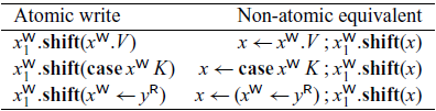
Each atomic write simply evaluates in a single step to the configuration where both x and $x_1$
have been written to, much as if the non-atomic equivalent had taken three steps — first for the cut, second to write to x, and third to write to
$x_1$
have been written to, much as if the non-atomic equivalent had taken three steps — first for the cut, second to write to x, and third to write to $x_1$
. This intuition is formalized in the following transition rules:
$x_1$
. This intuition is formalized in the following transition rules:

Note that the rule for the identity case is different from the other two — it requires the cell $y_k$
to have been written to in order to continue. This is because the
$y_k$
to have been written to in order to continue. This is because the $x^{{\mathchoice{\textsf{W}}{\textsf{W}}{\scriptscriptstyle\textsf{W}}{\scriptscriptstyle\textsf{W}}}} \leftarrow y^{{\mathchoice{\textsf{R}}{\textsf{R}}{\scriptscriptstyle\textsf{R}}{\scriptscriptstyle\textsf{R}}}}$
construct reads from y and writes to x — if we wish to write to x and
$x^{{\mathchoice{\textsf{W}}{\textsf{W}}{\scriptscriptstyle\textsf{W}}{\scriptscriptstyle\textsf{W}}}} \leftarrow y^{{\mathchoice{\textsf{R}}{\textsf{R}}{\scriptscriptstyle\textsf{R}}{\scriptscriptstyle\textsf{R}}}}$
construct reads from y and writes to x — if we wish to write to x and $x_1$
atomically, we must also perform the read from y.
$x_1$
atomically, we must also perform the read from y.
Now, to obtain P’ from P, we define a substitution operation $[x_1.\mathbf{shift}(x) // x]$
that replaces writes to x with atomic writes to x and
$[x_1.\mathbf{shift}(x) // x]$
that replaces writes to x with atomic writes to x and $x_1$
as follows:
$x_1$
as follows:
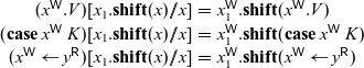 \begin{equation*}\begin{array}{rcl}(x^{{\mathchoice{\textsf{W}}{\textsf{W}}{\scriptscriptstyle\textsf{W}}{\scriptscriptstyle\textsf{W}}}}.V)[x_1.\mathbf{shift}(x) // x] &=& x_1^{{\mathchoice{\textsf{W}}{\textsf{W}}{\scriptscriptstyle\textsf{W}}{\scriptscriptstyle\textsf{W}}}}.\mathbf{shift}(x^{{\mathchoice{\textsf{W}}{\textsf{W}}{\scriptscriptstyle\textsf{W}}{\scriptscriptstyle\textsf{W}}}}.V) \\(\mathbf{case}\; x^{{\mathchoice{\textsf{W}}{\textsf{W}}{\scriptscriptstyle\textsf{W}}{\scriptscriptstyle\textsf{W}}}}\; K)[x_1.\mathbf{shift}(x) // x] &=& x_1^{{\mathchoice{\textsf{W}}{\textsf{W}}{\scriptscriptstyle\textsf{W}}{\scriptscriptstyle\textsf{W}}}}.\mathbf{shift}(\mathbf{case}\; x^{{\mathchoice{\textsf{W}}{\textsf{W}}{\scriptscriptstyle\textsf{W}}{\scriptscriptstyle\textsf{W}}}}\; K) \\(x^{{\mathchoice{\textsf{W}}{\textsf{W}}{\scriptscriptstyle\textsf{W}}{\scriptscriptstyle\textsf{W}}}} \leftarrow y^{{\mathchoice{\textsf{R}}{\textsf{R}}{\scriptscriptstyle\textsf{R}}{\scriptscriptstyle\textsf{R}}}})[x_1.\mathbf{shift}(x) // x] &=& x_1^{{\mathchoice{\textsf{W}}{\textsf{W}}{\scriptscriptstyle\textsf{W}}{\scriptscriptstyle\textsf{W}}}}.\mathbf{shift}(x^{{\mathchoice{\textsf{W}}{\textsf{W}}{\scriptscriptstyle\textsf{W}}{\scriptscriptstyle\textsf{W}}}} \leftarrow y^{{\mathchoice{\textsf{R}}{\textsf{R}}{\scriptscriptstyle\textsf{R}}{\scriptscriptstyle\textsf{R}}}}) \\\end{array}\end{equation*}
Extending $[x_1.\mathbf{shift}(x) // x]$
compositionally over our other language constructs, we can define
$[x_1.\mathbf{shift}(x) // x]$
compositionally over our other language constructs, we can define $P' = P[x_1.\mathbf{shift}(x) // x]$
, and so
$P' = P[x_1.\mathbf{shift}(x) // x]$
, and so
 \begin{equation*}x \overset{\textsf{seq}}{\leftarrow} P \mathrel{;} Q \triangleq x_1 \leftarrow P[x_1.\mathbf{shift}(x) // x] \mathrel{;} \mathbf{case}\; x_1^{{\mathchoice{\textsf{R}}{\textsf{R}}{\scriptscriptstyle\textsf{R}}{\scriptscriptstyle\textsf{R}}}}\; (\mathbf{shift}(x) \Rightarrow Q).\end{equation*}
We now can use the sequential cut to enforce an order on computation. Of particular interest is the case where we restrict our language so that all cuts are sequential. This gives us a fully sequential language, where we indeed have that only one thread is active at a time. We will make extensive use of this ability to give a fully sequential language, and in Sections 7 and 9, we will add back limited access to concurrency to such a sequential language in order to reconstruct various patterns of concurrent computation.
There are a few properties of the operation $[x_1.\mathbf{shift}(x) // x]$
and the sequential cut that we will make use of in our embeddings. Essentially, we would like to know that
$[x_1.\mathbf{shift}(x) // x]$
and the sequential cut that we will make use of in our embeddings. Essentially, we would like to know that $P[x_1.\mathbf{shift}(x) // x]$
has similar behavior from a typing perspective to P, and that a sequential cut can be typed in a similar manner to a standard concurrent cut. We make this precise with the following lemmas:
$P[x_1.\mathbf{shift}(x) // x]$
has similar behavior from a typing perspective to P, and that a sequential cut can be typed in a similar manner to a standard concurrent cut. We make this precise with the following lemmas:
Lemma 4. If $\Gamma \vdash P :: (x : A_m)$
, then
$\Gamma \vdash P :: (x : A_m)$
, then $\Gamma \vdash P[x_1.\mathbf{shift}(x) // x] :: (x_1 : {\downarrow}^m_m A_m)$
.
$\Gamma \vdash P[x_1.\mathbf{shift}(x) // x] :: (x_1 : {\downarrow}^m_m A_m)$
.
Lemma 5. The rule
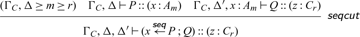
is admissible.
Lemma 4 follows from a simple induction on the structure of P, and Lemma 5 can be proven by deriving the $\textsf{seqcut}$
rule using Lemma 4.
$\textsf{seqcut}$
rule using Lemma 4.
In an earlier version of this paper, Footnote 7 we developed a separate set of sequential semantics which is bisimilar to the presentation we give here in terms of sequential cuts. However, by embedding the sequential cut into the concurrent semantics as syntactic sugar, we are able to drastically reduce the conceptual and technical overhead needed to look at interactions between the two different frameworks and simplify our encodings of various concurrency patterns.
Example revisited: $\lambda$
-calculus.
$\lambda$
-calculus.
If we make all cuts in the $\lambda$
-calculus interpreter sequential, we obtain a call-by-value semantics. In particular, it may no longer compute a weak head-normal form even if it exists. Note that just as we used syntactic sugar for standard cuts with the identity or call rule on the left, we will also define for convenience
$\lambda$
-calculus interpreter sequential, we obtain a call-by-value semantics. In particular, it may no longer compute a weak head-normal form even if it exists. Note that just as we used syntactic sugar for standard cuts with the identity or call rule on the left, we will also define for convenience
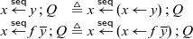 \begin{equation*} \begin{array}{lcll} x \overset{\textsf{seq}}{\leftarrow} y \mathrel{;} Q & \triangleq & x\overset{\textsf{seq}}{\leftarrow} (x \leftarrow y) \mathrel{;} Q \\ x \overset{\textsf{seq}}{\leftarrow} f \; \overline{y} \mathrel{;} Q & \triangleq & x \overset{\textsf{seq}}{\leftarrow} (x \leftarrow f \; \overline{y}) \mathrel{;} Q \end{array}\end{equation*}
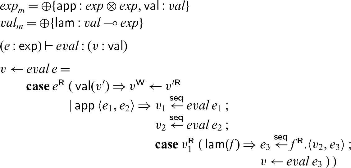
Call-by-name. As mentioned at the beginning of this section, there are multiple approaches to enforcing that only one thread is active at a time. We can think of the sequential cut defined in Section 5 as a form of call-by-value — P is fully evaluated before Q can continue. Here, we will define a different sequential cut $x \overset{N}{\leftarrow} P \mathrel{;} Q$
, which will behave more like call-by-name, delaying execution of P until Q attempts to read from x. Interestingly, this construct avoids the need for atomic write operations! We nevertheless prefer the “call-by-value” form of sequentiality as our default, as it aligns better with Halstead’s approach to futures (Halstead Reference Halstead1985), which were defined in a call-by-value language, and also avoids recomputing P if x is used multiple times in Q.
$x \overset{N}{\leftarrow} P \mathrel{;} Q$
, which will behave more like call-by-name, delaying execution of P until Q attempts to read from x. Interestingly, this construct avoids the need for atomic write operations! We nevertheless prefer the “call-by-value” form of sequentiality as our default, as it aligns better with Halstead’s approach to futures (Halstead Reference Halstead1985), which were defined in a call-by-value language, and also avoids recomputing P if x is used multiple times in Q.
As before, we take advantage of shifts for synchronization, here using an upwards shift rather than a downward one. If $x : A_m$
, we would like to define
$x : A_m$
, we would like to define
 \begin{equation*}x \overset{N}{\leftarrow} P \mathrel{;} Q \triangleq x_1 \leftarrow \mathbf{case}\; x_1^{{\mathchoice{\textsf{W}}{\textsf{W}}{\scriptscriptstyle\textsf{W}}{\scriptscriptstyle\textsf{W}}}}\;(\mathbf{shift}(x) \Rightarrow P) \mathrel{;} Q',\end{equation*}
where $x_1 : {\uparrow}_m^m A_m$
, and Q’ can be derived from Q by a replacement operation that turns each read from x in Q into a read from
$x_1 : {\uparrow}_m^m A_m$
, and Q’ can be derived from Q by a replacement operation that turns each read from x in Q into a read from $x_1$
, followed by a read from x. We can formalize the operation that takes Q to Q’ in a similar manner to
$x_1$
, followed by a read from x. We can formalize the operation that takes Q to Q’ in a similar manner to $[x_1.\mathbf{shift}(x) // x]$
. We will call this operation
$[x_1.\mathbf{shift}(x) // x]$
. We will call this operation $[x_1.\mathbf{shift}(x) \% x]$
, so
$[x_1.\mathbf{shift}(x) \% x]$
, so $Q' = Q[x_1.\mathbf{shift}(x) \% x]$
.
$Q' = Q[x_1.\mathbf{shift}(x) \% x]$
.
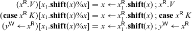 \begin{equation*}\begin{array}{rcl}(x^{{\mathchoice{\textsf{R}}{\textsf{R}}{\scriptscriptstyle\textsf{R}}{\scriptscriptstyle\textsf{R}}}}.V)[x_1.\mathbf{shift}(x) \% x] &=& x \leftarrow x_1^{{\mathchoice{\textsf{R}}{\textsf{R}}{\scriptscriptstyle\textsf{R}}{\scriptscriptstyle\textsf{R}}}}.\mathbf{shift}(x) \mathrel{;} x^{{\mathchoice{\textsf{R}}{\textsf{R}}{\scriptscriptstyle\textsf{R}}{\scriptscriptstyle\textsf{R}}}}.V \\(\mathbf{case}\; x^{{\mathchoice{\textsf{R}}{\textsf{R}}{\scriptscriptstyle\textsf{R}}{\scriptscriptstyle\textsf{R}}}}\; K)[x_1.\mathbf{shift}(x) \% x] &=& x \leftarrow x_1^{{\mathchoice{\textsf{R}}{\textsf{R}}{\scriptscriptstyle\textsf{R}}{\scriptscriptstyle\textsf{R}}}}.\mathbf{shift}(x) \mathrel{;} \mathbf{case}\; x^{{\mathchoice{\textsf{R}}{\textsf{R}}{\scriptscriptstyle\textsf{R}}{\scriptscriptstyle\textsf{R}}}}\; K \\(y^{{\mathchoice{\textsf{W}}{\textsf{W}}{\scriptscriptstyle\textsf{W}}{\scriptscriptstyle\textsf{W}}}} \leftarrow x^{{\mathchoice{\textsf{R}}{\textsf{R}}{\scriptscriptstyle\textsf{R}}{\scriptscriptstyle\textsf{R}}}})[x_1.\mathbf{shift}(x) \% x] &=& x \leftarrow x_1^{{\mathchoice{\textsf{R}}{\textsf{R}}{\scriptscriptstyle\textsf{R}}{\scriptscriptstyle\textsf{R}}}}.\mathbf{shift}(x) \mathrel{;} y^{{\mathchoice{\textsf{W}}{\textsf{W}}{\scriptscriptstyle\textsf{W}}{\scriptscriptstyle\textsf{W}}}} \leftarrow x^{{\mathchoice{\textsf{R}}{\textsf{R}}{\scriptscriptstyle\textsf{R}}{\scriptscriptstyle\textsf{R}}}} \\\end{array}\end{equation*}
Note that unlike in our “call-by-value” sequential cut, where we wrote to two cells atomically to ensure that one was written before the other, here, the order of reads is enforced because $x_1^{{\mathchoice{\textsf{R}}{\textsf{R}}{\scriptscriptstyle\textsf{R}}{\scriptscriptstyle\textsf{R}}}}.\mathbf{shift}(x)$
will execute the stored continuation
$x_1^{{\mathchoice{\textsf{R}}{\textsf{R}}{\scriptscriptstyle\textsf{R}}{\scriptscriptstyle\textsf{R}}}}.\mathbf{shift}(x)$
will execute the stored continuation $\mathbf{shift}(x) \Rightarrow P$
, which finishes by writing to x. As such, we are guaranteed that Q’ is paused waiting to read from x until P finishes executing. Moreover, P is paused within a continuation until Q’ reads from
$\mathbf{shift}(x) \Rightarrow P$
, which finishes by writing to x. As such, we are guaranteed that Q’ is paused waiting to read from x until P finishes executing. Moreover, P is paused within a continuation until Q’ reads from $x_1$
, after which it immediately blocks on x, so we maintain only one active thread as desired.
$x_1$
, after which it immediately blocks on x, so we maintain only one active thread as desired.
While we will not make much use of this form of sequentiality, we find it interesting that it is so simply encoded, and that the encoding is so similar to that of call-by-value cuts. Both constructions are also quite natural — the main decision that we make is whether to pause P or Q inside a continuation. From this, the rest of the construction follows, as there are two natural places to wake up the paused process — as early as possible or as late as possible. If we wake the paused process P immediately after the cut, as in
 \begin{equation*}x_1 \leftarrow \mathbf{case}\; x_1^{{\mathchoice{\textsf{W}}{\textsf{W}}{\scriptscriptstyle\textsf{W}}{\scriptscriptstyle\textsf{W}}}}\;(\mathbf{shift}(x) \Rightarrow P) \mathrel{;} x \leftarrow x_1^{{\mathchoice{\textsf{R}}{\textsf{R}}{\scriptscriptstyle\textsf{R}}{\scriptscriptstyle\textsf{R}}}}.\mathbf{shift}(x) \mathrel{;} Q,\end{equation*}
the result is a concurrent cut with the extra overhead of the shift. Our sequential cuts are the result of waking the paused process as late as possible — once there is no more work to be done in P in the call-by-value cut, and once Q starts to actually depend on the result of P in the call-by-name cut. $\lambda$
-Calculus example revisited. We can achieve a sequential interpreter for the
$\lambda$
-Calculus example revisited. We can achieve a sequential interpreter for the $\lambda$
-calculus with a single use of a by-name cut. This interpreter is then complete: if a weak head-normal form exists, it will compute it. We also recall that this property holds no matter which structural properties we allow for the
$\lambda$
-calculus with a single use of a by-name cut. This interpreter is then complete: if a weak head-normal form exists, it will compute it. We also recall that this property holds no matter which structural properties we allow for the $\lambda$
-calculus (e.g., purely linear if the mode allows neither weakening nor contraction, of the
$\lambda$
-calculus (e.g., purely linear if the mode allows neither weakening nor contraction, of the $\lambda I$
-calculus if the mode only allows contraction).
$\lambda I$
-calculus if the mode only allows contraction).
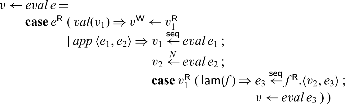
6 Functions
Rather than presenting an embedding or translation of a full (sequential) functional language into our system, we will focus on the case of functions. There is a standard translation of natural deduction to sequent calculus taking introduction rules to right rules, and constructing elimination rules from cut and left rules. We base our embedding of functions into our language on this translation. By following a similar process with other types, one can similarly embed other functional constructs, such as products and sums.
We will embed functions into an instance of Seax with a single mode m. For this example, we specify $\sigma(m) = \{W, C\}$
in order to model a typical functional language, but we could, for instance, take
$\sigma(m) = \{W, C\}$
in order to model a typical functional language, but we could, for instance, take $\sigma(m) = \{\}$
to model the linear
$\sigma(m) = \{\}$
to model the linear $\lambda$
-calculus. We also restrict the language at mode m to only have sequential cuts, which will allow us to better model a sequential language. Note that while we only specify one mode here, we could work within a larger mode structure, as long as it contains a suitable mode m at which to implement functions — namely, one with the appropriate structural properties, and where we have the restriction of only having sequential cuts. It is this modularity that allows us to freely combine the various reconstructions presented here and in the following sections. As we are only working within a single mode in this section, we will generally omit mode subscripts, but everything is implicitly at mode m.
$\lambda$
-calculus. We also restrict the language at mode m to only have sequential cuts, which will allow us to better model a sequential language. Note that while we only specify one mode here, we could work within a larger mode structure, as long as it contains a suitable mode m at which to implement functions — namely, one with the appropriate structural properties, and where we have the restriction of only having sequential cuts. It is this modularity that allows us to freely combine the various reconstructions presented here and in the following sections. As we are only working within a single mode in this section, we will generally omit mode subscripts, but everything is implicitly at mode m.
Now, to add functions to this language, we begin by adding a new type $A \to B$
and two new constructs — a constructor and a destructor for this type. The constructor,
$A \to B$
and two new constructs — a constructor and a destructor for this type. The constructor, $z^{{\mathchoice{\textsf{W}}{\textsf{W}}{\scriptscriptstyle\textsf{W}}{\scriptscriptstyle\textsf{W}}}}.(\lambda x . P_\star)$
, writes a
$z^{{\mathchoice{\textsf{W}}{\textsf{W}}{\scriptscriptstyle\textsf{W}}{\scriptscriptstyle\textsf{W}}}}.(\lambda x . P_\star)$
, writes a $\lambda$
-abstraction to destination z. Here, we write
$\lambda$
-abstraction to destination z. Here, we write $P_\star$
for a process expression P whose destination is
$P_\star$
for a process expression P whose destination is $\star$
. We will write
$\star$
. We will write $P_y$
for
$P_y$
for $P[y/\star]$
. The use of
$P[y/\star]$
. The use of $\star$
makes this closer to the standard functional style, where the location that the result is returned to is not made explicit. The destructor,
$\star$
makes this closer to the standard functional style, where the location that the result is returned to is not made explicit. The destructor, $P_\star(Q_\star)$
, applies the function
$P_\star(Q_\star)$
, applies the function $P_\star$
to
$P_\star$
to $Q_\star$
. These can be typed using variants of the standard
$Q_\star$
. These can be typed using variants of the standard $\to I$
and
$\to I$
and $\to E$
rules labeled with channels:
$\to E$
rules labeled with channels:

In order to avoid having to augment our language each time, we wish to add a new feature, we will show that these new constructs can be treated as syntactic sugar for terms already in the language, and, moreover, that those terms behave as we would expect of functions and function applications.
We take the following definitions for the new type and terms:
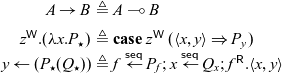 \begin{equation*}\begin{array}{rcl}A \to B &\triangleq& A \multimap B \\[1ex]z^{{\mathchoice{\textsf{W}}{\textsf{W}}{\scriptscriptstyle\textsf{W}}{\scriptscriptstyle\textsf{W}}}}.(\lambda x . P_\star) &\triangleq&\mathbf{case}\, z^{{\mathchoice{\textsf{W}}{\textsf{W}}{\scriptscriptstyle\textsf{W}}{\scriptscriptstyle\textsf{W}}}}\, (\langle x, y \rangle \Rightarrow P_y) \\y \leftarrow (P_\star(Q_\star)) &\triangleq&f \overset{\textsf{seq}}{\leftarrow} P_f ; x \overset{\textsf{seq}}{\leftarrow} Q_x ; f^{{\mathchoice{\textsf{R}}{\textsf{R}}{\scriptscriptstyle\textsf{R}}{\scriptscriptstyle\textsf{R}}}}.\langle x, y \rangle \\\end{array}\end{equation*}
These definitions are type-correct, as shown by the following theorem:
Theorem 6 If we expand all new constructs using $\triangleq$
, then the typing rules rules
$\triangleq$
, then the typing rules rules $\to I$
and
$\to I$
and $\to E$
above are admissible.
$\to E$
above are admissible.
We can prove this by deriving the typing rules, using Lemma 5 in a few places.
Now that we have established that we can expand this syntactic sugar for functions in a type-correct manner, we examine the evaluation behavior of these terms. First, we consider the lambda abstraction $z^{{\mathchoice{\textsf{W}}{\textsf{W}}{\scriptscriptstyle\textsf{W}}{\scriptscriptstyle\textsf{W}}}}.(\lambda x . P_\star)$
and its expansion
$z^{{\mathchoice{\textsf{W}}{\textsf{W}}{\scriptscriptstyle\textsf{W}}{\scriptscriptstyle\textsf{W}}}}.(\lambda x . P_\star)$
and its expansion $\mathbf{case}\, z^{{\mathchoice{\textsf{W}}{\textsf{W}}{\scriptscriptstyle\textsf{W}}{\scriptscriptstyle\textsf{W}}}}\, (\langle x, y \rangle \Rightarrow P_y)$
. A lambda abstraction should already be a value, and so we might expect that it can be written to memory immediately. Indeed, in the expansion, we immediately write the continuation
$\mathbf{case}\, z^{{\mathchoice{\textsf{W}}{\textsf{W}}{\scriptscriptstyle\textsf{W}}{\scriptscriptstyle\textsf{W}}}}\, (\langle x, y \rangle \Rightarrow P_y)$
. A lambda abstraction should already be a value, and so we might expect that it can be written to memory immediately. Indeed, in the expansion, we immediately write the continuation $(\langle x, y \rangle \Rightarrow P_y)$
, which serves as the analogue for
$(\langle x, y \rangle \Rightarrow P_y)$
, which serves as the analogue for $(\lambda x . P_\star)$
. This term thus behaves as expected.
$(\lambda x . P_\star)$
. This term thus behaves as expected.
We expect that when applying a function $P_\star$
to an argument
$P_\star$
to an argument $Q_\star$
, we first reduce
$Q_\star$
, we first reduce $P_\star$
to a value, then reduce
$P_\star$
to a value, then reduce $Q_\star$
to a value, and then apply the value of
$Q_\star$
to a value, and then apply the value of $P_\star$
to the value of
$P_\star$
to the value of $Q_\star$
, generally by substitution. In the term
$Q_\star$
, generally by substitution. In the term $f \overset{\textsf{seq}}{\leftarrow} P_f ; x \overset{\textsf{seq}}{\leftarrow} Q_x ; f^{{\mathchoice{\textsf{R}}{\textsf{R}}{\scriptscriptstyle\textsf{R}}{\scriptscriptstyle\textsf{R}}}}.\langle x, y \rangle$
, we see exactly this behavior. We first evaluate
$f \overset{\textsf{seq}}{\leftarrow} P_f ; x \overset{\textsf{seq}}{\leftarrow} Q_x ; f^{{\mathchoice{\textsf{R}}{\textsf{R}}{\scriptscriptstyle\textsf{R}}{\scriptscriptstyle\textsf{R}}}}.\langle x, y \rangle$
, we see exactly this behavior. We first evaluate $P_f$
into f, then
$P_f$
into f, then $Q_x$
into x, and then apply the continuation stored in f to the pair
$Q_x$
into x, and then apply the continuation stored in f to the pair $\langle x, y \rangle$
.
$\langle x, y \rangle$
.
7 Futures
Futures (Halstead Reference Halstead1985) are a classic example of a primitive to introduce concurrency into a sequential language. In the usual presentation, we add to a (sequential) functional language the ability to create a future that immediately returns a promise and spawns a concurrent computation. Touching a promise by trying to access its value blocks until that value has been computed. Futures have been a popular mechanism for parallel execution in both statically and dynamically typed languages, and they are also used to encapsulate various communication primitives.
The development of a sequential cut in Section 5 provides us with ways to model or reconstruct concurrency primitives, and futures are a surprisingly simple example of this. Starting with a language that only allows sequential cuts, we would like to add a new construct that serves to create a future, as we added functions to the base language in Section 6. In this case, however, we already have a construct that behaves exactly as desired. The concurrent cut $x \leftarrow P \mathrel{;} Q$
spawns a new process P and executes P and Q concurrently. When Q tries to read from x, it will block until P has computed a result W and written it to x. If we wish to add an explicit synchronization point, we can do so with minimal overhead by making use of identity to read from x. For instance, the process
$x \leftarrow P \mathrel{;} Q$
spawns a new process P and executes P and Q concurrently. When Q tries to read from x, it will block until P has computed a result W and written it to x. If we wish to add an explicit synchronization point, we can do so with minimal overhead by making use of identity to read from x. For instance, the process $z \leftarrow (z^{{\mathchoice{\textsf{W}}{\textsf{W}}{\scriptscriptstyle\textsf{W}}{\scriptscriptstyle\textsf{W}}}} \leftarrow x^{{\mathchoice{\textsf{R}}{\textsf{R}}{\scriptscriptstyle\textsf{R}}{\scriptscriptstyle\textsf{R}}}}) \mathrel{;} Q$
will first copy or move the contents of cell x to cell z, and then run Q. As such, it delays the execution of Q until x has been written to, even if Q does not need to look at the value of x until later. This is analogous to the touch construct of some approaches to futures.
$z \leftarrow (z^{{\mathchoice{\textsf{W}}{\textsf{W}}{\scriptscriptstyle\textsf{W}}{\scriptscriptstyle\textsf{W}}}} \leftarrow x^{{\mathchoice{\textsf{R}}{\textsf{R}}{\scriptscriptstyle\textsf{R}}{\scriptscriptstyle\textsf{R}}}}) \mathrel{;} Q$
will first copy or move the contents of cell x to cell z, and then run Q. As such, it delays the execution of Q until x has been written to, even if Q does not need to look at the value of x until later. This is analogous to the touch construct of some approaches to futures.
In other words, in this language, futures, rather than being a construct that we need to add and examine carefully, are in fact the default. This is, in a sense, opposite to the standard approach, where sequentiality is the norm and a new construct is needed to handle futures. By instead adding sequential cut to our otherwise concurrent language, we get the same expressive power, being able to specify whenever we spawn a new computation whether it should be run concurrently with or sequentially before the continuation process.
These futures, much like those in Halstead’s Multilisp, are not distinguished at the type level and do not require an explicit touch construct for synchronization, although we can add synchronization points as shown. It is possible to provide an encoding of futures with a distinct type, as they are used in many more modern languages (see Appendix 1), but we find the form presented here more natural, as it allows a great deal of flexibility to the programmer — a process using a variable x does not know and need not care whether the value of x is computed concurrently or not.
One interesting result that arises from this approach to futures, and in particular from the fact that this approach works at any mode m, regardless of what $\sigma(m)$
is, is that by considering the case where
$\sigma(m)$
is, is that by considering the case where $\sigma(m) = \{\}$
, we recover a definition of linear futures, which must be used exactly once. This is limited in that the base language at mode m will also be linear, along with its futures. However, we are not restricted to working with one mode. For instance, we may take a mode
$\sigma(m) = \{\}$
, we recover a definition of linear futures, which must be used exactly once. This is limited in that the base language at mode m will also be linear, along with its futures. However, we are not restricted to working with one mode. For instance, we may take a mode ${\mathchoice{\textsf{S}}{\textsf{S}}{\scriptscriptstyle\textsf{S}}{\scriptscriptstyle\textsf{S}}}$
with
${\mathchoice{\textsf{S}}{\textsf{S}}{\scriptscriptstyle\textsf{S}}{\scriptscriptstyle\textsf{S}}}$
with $\sigma({\mathchoice{\textsf{S}}{\textsf{S}}{\scriptscriptstyle\textsf{S}}{\scriptscriptstyle\textsf{S}}}) = \{\}$
, which allows for programming linearly with futures, and a mode
$\sigma({\mathchoice{\textsf{S}}{\textsf{S}}{\scriptscriptstyle\textsf{S}}{\scriptscriptstyle\textsf{S}}}) = \{\}$
, which allows for programming linearly with futures, and a mode ${\mathchoice{\textsf{S}}{\textsf{S}}{\scriptscriptstyle\textsf{S}}{\scriptscriptstyle\textsf{S}}}^*$
with
${\mathchoice{\textsf{S}}{\textsf{S}}{\scriptscriptstyle\textsf{S}}{\scriptscriptstyle\textsf{S}}}^*$
with $\sigma({\mathchoice{\textsf{S}}{\textsf{S}}{\scriptscriptstyle\textsf{S}}{\scriptscriptstyle\textsf{S}}}^*) = \{\textsf{W}, \textsf{C}\}$
and
$\sigma({\mathchoice{\textsf{S}}{\textsf{S}}{\scriptscriptstyle\textsf{S}}{\scriptscriptstyle\textsf{S}}}^*) = \{\textsf{W}, \textsf{C}\}$
and ${\mathchoice{\textsf{S}}{\textsf{S}}{\scriptscriptstyle\textsf{S}}{\scriptscriptstyle\textsf{S}}} < {\mathchoice{\textsf{S}}{\textsf{S}}{\scriptscriptstyle\textsf{S}}{\scriptscriptstyle\textsf{S}}}^*$
, which allows for standard functional programming. The shifts between the linear and non-linear modes allow both types of futures to be used in the same program, embedding the linear language (including its futures) into the non-linear language via the monad
${\mathchoice{\textsf{S}}{\textsf{S}}{\scriptscriptstyle\textsf{S}}{\scriptscriptstyle\textsf{S}}} < {\mathchoice{\textsf{S}}{\textsf{S}}{\scriptscriptstyle\textsf{S}}{\scriptscriptstyle\textsf{S}}}^*$
, which allows for standard functional programming. The shifts between the linear and non-linear modes allow both types of futures to be used in the same program, embedding the linear language (including its futures) into the non-linear language via the monad ${\uparrow}_{\mathchoice{\textsf{S}}{\textsf{S}}{\scriptscriptstyle\textsf{S}}{\scriptscriptstyle\textsf{S}}}^{{\mathchoice{\textsf{S}}{\textsf{S}}{\scriptscriptstyle\textsf{S}}{\scriptscriptstyle\textsf{S}}}^*} {\downarrow}^{{\mathchoice{\textsf{S}}{\textsf{S}}{\scriptscriptstyle\textsf{S}}{\scriptscriptstyle\textsf{S}}}^*}_{\mathchoice{\textsf{S}}{\textsf{S}}{\scriptscriptstyle\textsf{S}}{\scriptscriptstyle\textsf{S}}}$
. Uses for linear futures (without a full formalization) in the efficient expression of certain parallel algorithms have already been explored in prior work (Blelloch & Reid-Miller Reference Blelloch and Reid-Miller1999), but to our knowledge, no formalization of linear futures has yet been given.
${\uparrow}_{\mathchoice{\textsf{S}}{\textsf{S}}{\scriptscriptstyle\textsf{S}}{\scriptscriptstyle\textsf{S}}}^{{\mathchoice{\textsf{S}}{\textsf{S}}{\scriptscriptstyle\textsf{S}}{\scriptscriptstyle\textsf{S}}}^*} {\downarrow}^{{\mathchoice{\textsf{S}}{\textsf{S}}{\scriptscriptstyle\textsf{S}}{\scriptscriptstyle\textsf{S}}}^*}_{\mathchoice{\textsf{S}}{\textsf{S}}{\scriptscriptstyle\textsf{S}}{\scriptscriptstyle\textsf{S}}}$
. Uses for linear futures (without a full formalization) in the efficient expression of certain parallel algorithms have already been explored in prior work (Blelloch & Reid-Miller Reference Blelloch and Reid-Miller1999), but to our knowledge, no formalization of linear futures has yet been given.
Binary numbers revisited. The program for plus2 presented in Section 4.2 is a classic example of a (rather short-lived) pipeline set up with futures. For this to exhibit the expected parallelism, the individual succ process should also be concurrent in its recursive call.
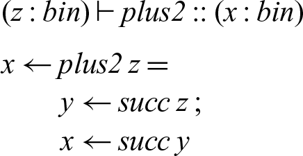
Simple variations (for example, setting up a Boolean circuit on bit streams) follow the same pattern of composition using futures.
mapReduce Revisited. As a use of futures, consider making all cuts in mapReduce sequential except those representing a recursive call:
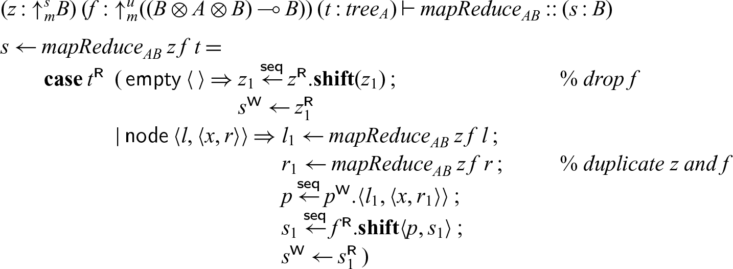
In this program, the computation at each node is sequential, but the two recursive calls to mapReduce are spawned as futures. We synchronize on these futures when they are needed in the computation of f.
8 Fork/Join parallelism
While futures allow us a great deal of freedom in writing concurrent programs with fine-grained control, sometimes it is useful to have a more restrictive concurrency primitive, either for implementation reasons or for reasoning about the behavior of programs. Fork/join parallelism is a simple, yet practically highly successful paradigm, allowing multiple independent threads to run in parallel, and then collecting the results together after those threads are finished, using a join construct. Many slightly different treatments of fork/join exist. Here, we will take as the primitive construct a parallel pair $\langle P_\star \mid Q_\star \rangle$
, which runs
$\langle P_\star \mid Q_\star \rangle$
, which runs $P_\star$
and
$P_\star$
and $Q_\star$
in parallel, and then stores the pair of results. Joining the computation then occurs when the pair is read from, which requires both
$Q_\star$
in parallel, and then stores the pair of results. Joining the computation then occurs when the pair is read from, which requires both $P_\star$
and
$P_\star$
and $Q_\star$
to have terminated. This form of fork/join is common in the literature dealing with scheduling and other optimizations for parallelism, particularly nested parallelism (e.g. Reference Acar, CharguÉraud, Guatto, Rainey and SieczkowskiAcar et al. (2018)), due to its relative simplicity.
$Q_\star$
to have terminated. This form of fork/join is common in the literature dealing with scheduling and other optimizations for parallelism, particularly nested parallelism (e.g. Reference Acar, CharguÉraud, Guatto, Rainey and SieczkowskiAcar et al. (2018)), due to its relative simplicity.
As with our reconstruction of functions in Section 6, we will use a single mode m which may have arbitrary structural properties, but only allows sequential cuts. As we are working with only a single mode, we will generally omit the subscripts that indicate mode, writing A rather than $A_m$
.
$A_m$
.
We introduce a new type $A_m \Vert B_m$
of parallel pairs and new terms to create and read from such pairs. We present these terms in the following typing rules:
$A_m \Vert B_m$
of parallel pairs and new terms to create and read from such pairs. We present these terms in the following typing rules:
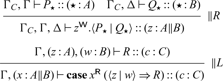
As in Section 6 we can reconstruct these types and terms in Seax already. Here, we define:
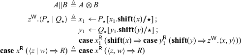 \begin{equation*}\begin{array}{rcl}A \Vert B &\triangleq&A \otimes B \\[1ex]z^{{\mathchoice{\textsf{W}}{\textsf{W}}{\scriptscriptstyle\textsf{W}}{\scriptscriptstyle\textsf{W}}}}.\langle P_\star \mid Q_\star \rangle &\triangleq&x_1 \leftarrow P_\star[x_1.\mathbf{shift}(x) // \star] \mathrel{;} \\&& y_1 \leftarrow Q_\star[y_1.\mathbf{shift}(y) // \star] \mathrel{;} \\&& \mathbf{case}\; x_1^{{\mathchoice{\textsf{R}}{\textsf{R}}{\scriptscriptstyle\textsf{R}}{\scriptscriptstyle\textsf{R}}}}\; (\mathbf{shift}(x) \Rightarrow \mathbf{case}\; y_1^{{\mathchoice{\textsf{R}}{\textsf{R}}{\scriptscriptstyle\textsf{R}}{\scriptscriptstyle\textsf{R}}}}\; (\mathbf{shift}(y) \Rightarrow z^{{\mathchoice{\textsf{W}}{\textsf{W}}{\scriptscriptstyle\textsf{W}}{\scriptscriptstyle\textsf{W}}}}.\langle x, y \rangle )) \\\mathbf{case}\; x^{{\mathchoice{\textsf{R}}{\textsf{R}}{\scriptscriptstyle\textsf{R}}{\scriptscriptstyle\textsf{R}}}}\; (\langle z \mid w \rangle \Rightarrow R) &\triangleq&\mathbf{case}\; x^{{\mathchoice{\textsf{R}}{\textsf{R}}{\scriptscriptstyle\textsf{R}}{\scriptscriptstyle\textsf{R}}}}\; (\langle z, w \rangle \Rightarrow R)\\\end{array}\end{equation*}
This definition respects the typing as prescribed by the $\Vert R$
and
$\Vert R$
and $\Vert L$
rules.
$\Vert L$
rules.
Theorem 7 If we expand all new constructs using $\triangleq$
, then the
$\triangleq$
, then the $\Vert R$
and
$\Vert R$
and $\Vert L$
rules above are admissible.
$\Vert L$
rules above are admissible.
This theorem follows quite straightforwardly from Lemma 4.
The evaluation behavior of these parallel pairs is quite simple — we first observe that, as the derivation of $\Vert L$
in the theorem above suggests, the reader of a parallel pair behaves exactly as the reader of an ordinary pair. The only difference, then, is in the synchronization behavior of the writer of the pair. Examining the term
$\Vert L$
in the theorem above suggests, the reader of a parallel pair behaves exactly as the reader of an ordinary pair. The only difference, then, is in the synchronization behavior of the writer of the pair. Examining the term
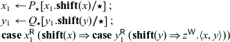 \begin{equation*}\begin{array}{l}x_1 \leftarrow P_\star[x_1.\mathbf{shift}(x) // \star] \mathrel{;} \\y_1 \leftarrow Q_\star[y_1.\mathbf{shift}(y) // \star] \mathrel{;} \\\mathbf{case}\; x_1^{{\mathchoice{\textsf{R}}{\textsf{R}}{\scriptscriptstyle\textsf{R}}{\scriptscriptstyle\textsf{R}}}}\; (\mathbf{shift}(x) \Rightarrow \mathbf{case}\; y_1^{{\mathchoice{\textsf{R}}{\textsf{R}}{\scriptscriptstyle\textsf{R}}{\scriptscriptstyle\textsf{R}}}}\; (\mathbf{shift}(y) \Rightarrow z^{{\mathchoice{\textsf{W}}{\textsf{W}}{\scriptscriptstyle\textsf{W}}{\scriptscriptstyle\textsf{W}}}}.\langle x, y \rangle )) \\\end{array}\end{equation*}
we see that it spawns two new threads, which run concurrently with the original thread. The new threads execute $P_\star[x_1.\mathbf{shift}(x) // \star]$
and
$P_\star[x_1.\mathbf{shift}(x) // \star]$
and $Q_\star[y_1.\mathbf{shift}(y) // \star]$
with destinations
$Q_\star[y_1.\mathbf{shift}(y) // \star]$
with destinations $x_1$
and
$x_1$
and $y_1$
, respectively, while the original thread waits first on
$y_1$
, respectively, while the original thread waits first on $x_1$
, then on
$x_1$
, then on $y_1$
, before writing the pair
$y_1$
, before writing the pair $\langle x, y \rangle$
to z. Because the new threads will write to x and
$\langle x, y \rangle$
to z. Because the new threads will write to x and $x_1$
atomically, and similarly for y and
$x_1$
atomically, and similarly for y and $y_1$
, by the time
$y_1$
, by the time $\langle x, y \rangle$
is written to z, x and y must have already been written to. However, because both cuts in this term are concurrent cuts,
$\langle x, y \rangle$
is written to z, x and y must have already been written to. However, because both cuts in this term are concurrent cuts, $P_\star$
and
$P_\star$
and $Q_\star$
run concurrently, as we expect from a parallel pair.
$Q_\star$
run concurrently, as we expect from a parallel pair.
mapReduce Revisited. We can use the fork/join pattern in the implementation of mapReduce so that we first synchronize on the results returned from the two recursive calls before we call f on them.
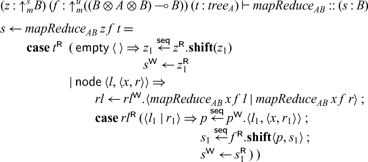
9 Monadic concurrency
For a different type of concurrency primitive, we look at a monad for concurrency, taking some inspiration from SILL (Toninho et al. Reference Toninho, Caires and Pfenning2013; Toninho Reference Toninho2015; Griffith Reference Griffith2016), which makes use of a contextual monad to embed the concurrency primitives of linear session types into a functional language. This allows us to have both a fully-featured sequential functional language and a fully-featured concurrent linear language, with the concurrent layer able to refer on variables in the sequential layer, but not the other way around. By keeping the layers separate in this way, we can reason about them independently. Moreover, the sequential layer could be implemented more simply than the concurrent layer — while the concurrent layer needs some form of locking or synchronization to ensure that a cell is not read from until it has been written to, the sequential layer can avoid all of this overhead. Similarly, while in the sequential layer, an implementation could avoid the extra work of thread management by maintaining a single thread.
To construct this concurrency monad, we will use two modes ${\mathchoice{\textsf{N}}{\textsf{N}}{\scriptscriptstyle\textsf{N}}{\scriptscriptstyle\textsf{N}}}$
and
${\mathchoice{\textsf{N}}{\textsf{N}}{\scriptscriptstyle\textsf{N}}{\scriptscriptstyle\textsf{N}}}$
and ${\mathchoice{\textsf{S}}{\textsf{S}}{\scriptscriptstyle\textsf{S}}{\scriptscriptstyle\textsf{S}}}$
with
${\mathchoice{\textsf{S}}{\textsf{S}}{\scriptscriptstyle\textsf{S}}{\scriptscriptstyle\textsf{S}}}$
with ${\mathchoice{\textsf{N}}{\textsf{N}}{\scriptscriptstyle\textsf{N}}{\scriptscriptstyle\textsf{N}}} < {\mathchoice{\textsf{S}}{\textsf{S}}{\scriptscriptstyle\textsf{S}}{\scriptscriptstyle\textsf{S}}}$
. Intuitively, the linear concurrent portion of the language is at mode
${\mathchoice{\textsf{N}}{\textsf{N}}{\scriptscriptstyle\textsf{N}}{\scriptscriptstyle\textsf{N}}} < {\mathchoice{\textsf{S}}{\textsf{S}}{\scriptscriptstyle\textsf{S}}{\scriptscriptstyle\textsf{S}}}$
. Intuitively, the linear concurrent portion of the language is at mode ${\mathchoice{\textsf{N}}{\textsf{N}}{\scriptscriptstyle\textsf{N}}{\scriptscriptstyle\textsf{N}}}$
, while the functional portion is at mode
${\mathchoice{\textsf{N}}{\textsf{N}}{\scriptscriptstyle\textsf{N}}{\scriptscriptstyle\textsf{N}}}$
, while the functional portion is at mode ${\mathchoice{\textsf{S}}{\textsf{S}}{\scriptscriptstyle\textsf{S}}{\scriptscriptstyle\textsf{S}}}$
. As in common in functional languages,
${\mathchoice{\textsf{S}}{\textsf{S}}{\scriptscriptstyle\textsf{S}}{\scriptscriptstyle\textsf{S}}}$
. As in common in functional languages, ${\mathchoice{\textsf{S}}{\textsf{S}}{\scriptscriptstyle\textsf{S}}{\scriptscriptstyle\textsf{S}}}$
allows weakening and contraction (
${\mathchoice{\textsf{S}}{\textsf{S}}{\scriptscriptstyle\textsf{S}}{\scriptscriptstyle\textsf{S}}}$
allows weakening and contraction ( $\sigma({\mathchoice{\textsf{S}}{\textsf{S}}{\scriptscriptstyle\textsf{S}}{\scriptscriptstyle\textsf{S}}}) = \{W,C\}$
), but only permits sequential cuts (by which we mean that any cut whose principal formula is at mode
$\sigma({\mathchoice{\textsf{S}}{\textsf{S}}{\scriptscriptstyle\textsf{S}}{\scriptscriptstyle\textsf{S}}}) = \{W,C\}$
), but only permits sequential cuts (by which we mean that any cut whose principal formula is at mode ${\mathchoice{\textsf{S}}{\textsf{S}}{\scriptscriptstyle\textsf{S}}{\scriptscriptstyle\textsf{S}}}$
must be a sequential cut) so that it models a sequential functional language. By contrast,
${\mathchoice{\textsf{S}}{\textsf{S}}{\scriptscriptstyle\textsf{S}}{\scriptscriptstyle\textsf{S}}}$
must be a sequential cut) so that it models a sequential functional language. By contrast, ${\mathchoice{\textsf{N}}{\textsf{N}}{\scriptscriptstyle\textsf{N}}{\scriptscriptstyle\textsf{N}}}$
allows concurrent cuts, but is linear (
${\mathchoice{\textsf{N}}{\textsf{N}}{\scriptscriptstyle\textsf{N}}{\scriptscriptstyle\textsf{N}}}$
allows concurrent cuts, but is linear ( $\sigma({\mathchoice{\textsf{S}}{\textsf{S}}{\scriptscriptstyle\textsf{S}}{\scriptscriptstyle\textsf{S}}}) = \{\}$
). We will write
$\sigma({\mathchoice{\textsf{S}}{\textsf{S}}{\scriptscriptstyle\textsf{S}}{\scriptscriptstyle\textsf{S}}}) = \{\}$
). We will write $A_{\mathchoice{\textsf{S}}{\textsf{S}}{\scriptscriptstyle\textsf{S}}{\scriptscriptstyle\textsf{S}}}$
and
$A_{\mathchoice{\textsf{S}}{\textsf{S}}{\scriptscriptstyle\textsf{S}}{\scriptscriptstyle\textsf{S}}}$
and $A_{\mathchoice{\textsf{N}}{\textsf{N}}{\scriptscriptstyle\textsf{N}}{\scriptscriptstyle\textsf{N}}}$
for sequential and concurrent types, respectively.
$A_{\mathchoice{\textsf{N}}{\textsf{N}}{\scriptscriptstyle\textsf{N}}{\scriptscriptstyle\textsf{N}}}$
for sequential and concurrent types, respectively.
The basic operations that we need, embedding concurrent processes in the functional layer and functional values in the concurrent layer, are simply the shifts ${\uparrow}_{\mathchoice{\textsf{N}}{\textsf{N}}{\scriptscriptstyle\textsf{N}}{\scriptscriptstyle\textsf{N}}}^{\mathchoice{\textsf{S}}{\textsf{S}}{\scriptscriptstyle\textsf{S}}{\scriptscriptstyle\textsf{S}}}$
and
${\uparrow}_{\mathchoice{\textsf{N}}{\textsf{N}}{\scriptscriptstyle\textsf{N}}{\scriptscriptstyle\textsf{N}}}^{\mathchoice{\textsf{S}}{\textsf{S}}{\scriptscriptstyle\textsf{S}}{\scriptscriptstyle\textsf{S}}}$
and ${\downarrow}^{\mathchoice{\textsf{S}}{\textsf{S}}{\scriptscriptstyle\textsf{S}}{\scriptscriptstyle\textsf{S}}}_{\mathchoice{\textsf{N}}{\textsf{N}}{\scriptscriptstyle\textsf{N}}{\scriptscriptstyle\textsf{N}}}$
, respectively. Composing these then yields a monad
${\downarrow}^{\mathchoice{\textsf{S}}{\textsf{S}}{\scriptscriptstyle\textsf{S}}{\scriptscriptstyle\textsf{S}}}_{\mathchoice{\textsf{N}}{\textsf{N}}{\scriptscriptstyle\textsf{N}}{\scriptscriptstyle\textsf{N}}}$
, respectively. Composing these then yields a monad ${\uparrow}_{\mathchoice{\textsf{N}}{\textsf{N}}{\scriptscriptstyle\textsf{N}}{\scriptscriptstyle\textsf{N}}}^{\mathchoice{\textsf{S}}{\textsf{S}}{\scriptscriptstyle\textsf{S}}{\scriptscriptstyle\textsf{S}}} {\downarrow}^{\mathchoice{\textsf{S}}{\textsf{S}}{\scriptscriptstyle\textsf{S}}{\scriptscriptstyle\textsf{S}}}_{\mathchoice{\textsf{N}}{\textsf{N}}{\scriptscriptstyle\textsf{N}}{\scriptscriptstyle\textsf{N}}} A_{\mathchoice{\textsf{S}}{\textsf{S}}{\scriptscriptstyle\textsf{S}}{\scriptscriptstyle\textsf{S}}}$
, with cell data of this type being a stored concurrent process which, when evaluated, yields a a functional value of type
${\uparrow}_{\mathchoice{\textsf{N}}{\textsf{N}}{\scriptscriptstyle\textsf{N}}{\scriptscriptstyle\textsf{N}}}^{\mathchoice{\textsf{S}}{\textsf{S}}{\scriptscriptstyle\textsf{S}}{\scriptscriptstyle\textsf{S}}} {\downarrow}^{\mathchoice{\textsf{S}}{\textsf{S}}{\scriptscriptstyle\textsf{S}}{\scriptscriptstyle\textsf{S}}}_{\mathchoice{\textsf{N}}{\textsf{N}}{\scriptscriptstyle\textsf{N}}{\scriptscriptstyle\textsf{N}}} A_{\mathchoice{\textsf{S}}{\textsf{S}}{\scriptscriptstyle\textsf{S}}{\scriptscriptstyle\textsf{S}}}$
, with cell data of this type being a stored concurrent process which, when evaluated, yields a a functional value of type $A_{\mathchoice{\textsf{S}}{\textsf{S}}{\scriptscriptstyle\textsf{S}}{\scriptscriptstyle\textsf{S}}}$
, tagged with a shift.
$A_{\mathchoice{\textsf{S}}{\textsf{S}}{\scriptscriptstyle\textsf{S}}{\scriptscriptstyle\textsf{S}}}$
, tagged with a shift.
To illustrate how this can be used for programming, we will present implementations of some of the features of SILL in this instance of Seax. SILL uses the type $\{ A_{\mathchoice{\textsf{N}}{\textsf{N}}{\scriptscriptstyle\textsf{N}}{\scriptscriptstyle\textsf{N}}} \}$
to lift processes from the concurrent layer to the functional layer, and types
$\{ A_{\mathchoice{\textsf{N}}{\textsf{N}}{\scriptscriptstyle\textsf{N}}{\scriptscriptstyle\textsf{N}}} \}$
to lift processes from the concurrent layer to the functional layer, and types $A_{\mathchoice{\textsf{S}}{\textsf{S}}{\scriptscriptstyle\textsf{S}}{\scriptscriptstyle\textsf{S}}} \land B_{\mathchoice{\textsf{N}}{\textsf{N}}{\scriptscriptstyle\textsf{N}}{\scriptscriptstyle\textsf{N}}}$
and
$A_{\mathchoice{\textsf{S}}{\textsf{S}}{\scriptscriptstyle\textsf{S}}{\scriptscriptstyle\textsf{S}}} \land B_{\mathchoice{\textsf{N}}{\textsf{N}}{\scriptscriptstyle\textsf{N}}{\scriptscriptstyle\textsf{N}}}$
and $A_{\mathchoice{\textsf{S}}{\textsf{S}}{\scriptscriptstyle\textsf{S}}{\scriptscriptstyle\textsf{S}}} \supset B_{\mathchoice{\textsf{N}}{\textsf{N}}{\scriptscriptstyle\textsf{N}}{\scriptscriptstyle\textsf{N}}}$
to send and receive functional values in the concurrent layer, respectively. Sending and receiving in a message-passing setting have analogs in writing values and continuations in Seax. For instance, rather than sending an
$A_{\mathchoice{\textsf{S}}{\textsf{S}}{\scriptscriptstyle\textsf{S}}{\scriptscriptstyle\textsf{S}}} \supset B_{\mathchoice{\textsf{N}}{\textsf{N}}{\scriptscriptstyle\textsf{N}}{\scriptscriptstyle\textsf{N}}}$
to send and receive functional values in the concurrent layer, respectively. Sending and receiving in a message-passing setting have analogs in writing values and continuations in Seax. For instance, rather than sending an $A_{\mathchoice{\textsf{S}}{\textsf{S}}{\scriptscriptstyle\textsf{S}}{\scriptscriptstyle\textsf{S}}}$
and continuing as
$A_{\mathchoice{\textsf{S}}{\textsf{S}}{\scriptscriptstyle\textsf{S}}{\scriptscriptstyle\textsf{S}}}$
and continuing as $B_{\mathchoice{\textsf{N}}{\textsf{N}}{\scriptscriptstyle\textsf{N}}{\scriptscriptstyle\textsf{N}}}$
, a process in Seax with type
$B_{\mathchoice{\textsf{N}}{\textsf{N}}{\scriptscriptstyle\textsf{N}}{\scriptscriptstyle\textsf{N}}}$
, a process in Seax with type $A_{\mathchoice{\textsf{S}}{\textsf{S}}{\scriptscriptstyle\textsf{S}}{\scriptscriptstyle\textsf{S}}} \land B_{\mathchoice{\textsf{N}}{\textsf{N}}{\scriptscriptstyle\textsf{N}}{\scriptscriptstyle\textsf{N}}}$
will write a pair of addresses pointing to an
$A_{\mathchoice{\textsf{S}}{\textsf{S}}{\scriptscriptstyle\textsf{S}}{\scriptscriptstyle\textsf{S}}} \land B_{\mathchoice{\textsf{N}}{\textsf{N}}{\scriptscriptstyle\textsf{N}}{\scriptscriptstyle\textsf{N}}}$
will write a pair of addresses pointing to an $A_{\mathchoice{\textsf{S}}{\textsf{S}}{\scriptscriptstyle\textsf{S}}{\scriptscriptstyle\textsf{S}}}$
and a
$A_{\mathchoice{\textsf{S}}{\textsf{S}}{\scriptscriptstyle\textsf{S}}{\scriptscriptstyle\textsf{S}}}$
and a $B_{\mathchoice{\textsf{N}}{\textsf{N}}{\scriptscriptstyle\textsf{N}}{\scriptscriptstyle\textsf{N}}}$
.
$B_{\mathchoice{\textsf{N}}{\textsf{N}}{\scriptscriptstyle\textsf{N}}{\scriptscriptstyle\textsf{N}}}$
.
The type $\{ A_{\mathchoice{\textsf{N}}{\textsf{N}}{\scriptscriptstyle\textsf{N}}{\scriptscriptstyle\textsf{N}}} \}$
of SILL has as values process expressions
$\{ A_{\mathchoice{\textsf{N}}{\textsf{N}}{\scriptscriptstyle\textsf{N}}{\scriptscriptstyle\textsf{N}}} \}$
of SILL has as values process expressions $\{ P_\star\}$
such that
$\{ P_\star\}$
such that ${P_\star :: (\star : A_{\mathchoice{\textsf{N}}{\textsf{N}}{\scriptscriptstyle\textsf{N}}{\scriptscriptstyle\textsf{N}}})}$
. These process expressions can be constructed and passed around in the functional layer. In order to actually execute these processes, however, we need to use a bind construct
${P_\star :: (\star : A_{\mathchoice{\textsf{N}}{\textsf{N}}{\scriptscriptstyle\textsf{N}}{\scriptscriptstyle\textsf{N}}})}$
. These process expressions can be constructed and passed around in the functional layer. In order to actually execute these processes, however, we need to use a bind construct $\{c_{\mathchoice{\textsf{N}}{\textsf{N}}{\scriptscriptstyle\textsf{N}}{\scriptscriptstyle\textsf{N}}}\} \leftarrow Q_\star$
in the functional layer, which will evaluate
$\{c_{\mathchoice{\textsf{N}}{\textsf{N}}{\scriptscriptstyle\textsf{N}}{\scriptscriptstyle\textsf{N}}}\} \leftarrow Q_\star$
in the functional layer, which will evaluate $Q_\star$
into an encapsulated process expression
$Q_\star$
into an encapsulated process expression $\{P_\star\}$
and then run
$\{P_\star\}$
and then run $P_\star$
, storing its result in
$P_\star$
, storing its result in $c_{\mathchoice{\textsf{N}}{\textsf{N}}{\scriptscriptstyle\textsf{N}}{\scriptscriptstyle\textsf{N}}}$
. We can add
$c_{\mathchoice{\textsf{N}}{\textsf{N}}{\scriptscriptstyle\textsf{N}}{\scriptscriptstyle\textsf{N}}}$
. We can add $\{\cdot\}$
to our language with the typing rules below. Here,
$\{\cdot\}$
to our language with the typing rules below. Here, $\Gamma_{\mathchoice{\textsf{S}}{\textsf{S}}{\scriptscriptstyle\textsf{S}}{\scriptscriptstyle\textsf{S}}}$
indicates that all assumptions in
$\Gamma_{\mathchoice{\textsf{S}}{\textsf{S}}{\scriptscriptstyle\textsf{S}}{\scriptscriptstyle\textsf{S}}}$
indicates that all assumptions in $\Gamma$
are at mode
$\Gamma$
are at mode ${\mathchoice{\textsf{S}}{\textsf{S}}{\scriptscriptstyle\textsf{S}}{\scriptscriptstyle\textsf{S}}}$
:
${\mathchoice{\textsf{S}}{\textsf{S}}{\scriptscriptstyle\textsf{S}}{\scriptscriptstyle\textsf{S}}}$
:

Since they live in the session-typed layer, the $\land$
and
$\land$
and $\supset$
constructs fit more straightforwardly into our language. We will focus on the type
$\supset$
constructs fit more straightforwardly into our language. We will focus on the type $A_{\mathchoice{\textsf{S}}{\textsf{S}}{\scriptscriptstyle\textsf{S}}{\scriptscriptstyle\textsf{S}}} \land B_{\mathchoice{\textsf{N}}{\textsf{N}}{\scriptscriptstyle\textsf{N}}{\scriptscriptstyle\textsf{N}}}$
, but
$A_{\mathchoice{\textsf{S}}{\textsf{S}}{\scriptscriptstyle\textsf{S}}{\scriptscriptstyle\textsf{S}}} \land B_{\mathchoice{\textsf{N}}{\textsf{N}}{\scriptscriptstyle\textsf{N}}{\scriptscriptstyle\textsf{N}}}$
, but $A_{\mathchoice{\textsf{S}}{\textsf{S}}{\scriptscriptstyle\textsf{S}}{\scriptscriptstyle\textsf{S}}} \supset B_{\mathchoice{\textsf{N}}{\textsf{N}}{\scriptscriptstyle\textsf{N}}{\scriptscriptstyle\textsf{N}}}$
can be handled similarly. A process of type
$A_{\mathchoice{\textsf{S}}{\textsf{S}}{\scriptscriptstyle\textsf{S}}{\scriptscriptstyle\textsf{S}}} \supset B_{\mathchoice{\textsf{N}}{\textsf{N}}{\scriptscriptstyle\textsf{N}}{\scriptscriptstyle\textsf{N}}}$
can be handled similarly. A process of type $A_{\mathchoice{\textsf{S}}{\textsf{S}}{\scriptscriptstyle\textsf{S}}{\scriptscriptstyle\textsf{S}}} \land B_{\mathchoice{\textsf{N}}{\textsf{N}}{\scriptscriptstyle\textsf{N}}{\scriptscriptstyle\textsf{N}}}$
writes a pair of a functional value with type
$A_{\mathchoice{\textsf{S}}{\textsf{S}}{\scriptscriptstyle\textsf{S}}{\scriptscriptstyle\textsf{S}}} \land B_{\mathchoice{\textsf{N}}{\textsf{N}}{\scriptscriptstyle\textsf{N}}{\scriptscriptstyle\textsf{N}}}$
writes a pair of a functional value with type $A_{\mathchoice{\textsf{S}}{\textsf{S}}{\scriptscriptstyle\textsf{S}}{\scriptscriptstyle\textsf{S}}}$
and a concurrent value with type
$A_{\mathchoice{\textsf{S}}{\textsf{S}}{\scriptscriptstyle\textsf{S}}{\scriptscriptstyle\textsf{S}}}$
and a concurrent value with type $B_{\mathchoice{\textsf{N}}{\textsf{N}}{\scriptscriptstyle\textsf{N}}{\scriptscriptstyle\textsf{N}}}$
. These terms and their typing rules are shown below:
$B_{\mathchoice{\textsf{N}}{\textsf{N}}{\scriptscriptstyle\textsf{N}}{\scriptscriptstyle\textsf{N}}}$
. These terms and their typing rules are shown below:
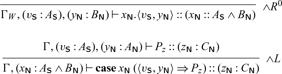
To show that these constructs can be expressed in the base language, we define
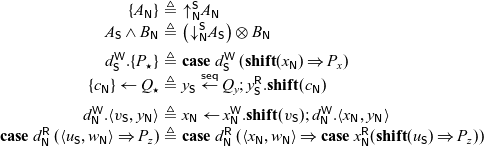 \begin{equation*}\begin{array}{rcl}\{A_{\mathchoice{\textsf{N}}{\textsf{N}}{\scriptscriptstyle\textsf{N}}{\scriptscriptstyle\textsf{N}}}\} &\triangleq& {\uparrow}_{\mathchoice{\textsf{N}}{\textsf{N}}{\scriptscriptstyle\textsf{N}}{\scriptscriptstyle\textsf{N}}}^{\mathchoice{\textsf{S}}{\textsf{S}}{\scriptscriptstyle\textsf{S}}{\scriptscriptstyle\textsf{S}}} A_{\mathchoice{\textsf{N}}{\textsf{N}}{\scriptscriptstyle\textsf{N}}{\scriptscriptstyle\textsf{N}}} \\A_{\mathchoice{\textsf{S}}{\textsf{S}}{\scriptscriptstyle\textsf{S}}{\scriptscriptstyle\textsf{S}}} \land B_{\mathchoice{\textsf{N}}{\textsf{N}}{\scriptscriptstyle\textsf{N}}{\scriptscriptstyle\textsf{N}}} &\triangleq& \left({\downarrow}^{\mathchoice{\textsf{S}}{\textsf{S}}{\scriptscriptstyle\textsf{S}}{\scriptscriptstyle\textsf{S}}}_{\mathchoice{\textsf{N}}{\textsf{N}}{\scriptscriptstyle\textsf{N}}{\scriptscriptstyle\textsf{N}}} A_{\mathchoice{\textsf{S}}{\textsf{S}}{\scriptscriptstyle\textsf{S}}{\scriptscriptstyle\textsf{S}}}\right) \otimes B_{\mathchoice{\textsf{N}}{\textsf{N}}{\scriptscriptstyle\textsf{N}}{\scriptscriptstyle\textsf{N}}} \\[1ex]d_{\mathchoice{\textsf{S}}{\textsf{S}}{\scriptscriptstyle\textsf{S}}{\scriptscriptstyle\textsf{S}}}^{{\mathchoice{\textsf{W}}{\textsf{W}}{\scriptscriptstyle\textsf{W}}{\scriptscriptstyle\textsf{W}}}}.\{P_\star\} &\triangleq&\mathbf{case}\; d_{\mathchoice{\textsf{S}}{\textsf{S}}{\scriptscriptstyle\textsf{S}}{\scriptscriptstyle\textsf{S}}}^{{\mathchoice{\textsf{W}}{\textsf{W}}{\scriptscriptstyle\textsf{W}}{\scriptscriptstyle\textsf{W}}}}\; (\mathbf{shift}(x_{\mathchoice{\textsf{N}}{\textsf{N}}{\scriptscriptstyle\textsf{N}}{\scriptscriptstyle\textsf{N}}}) \Rightarrow P_x) \\\{c_{\mathchoice{\textsf{N}}{\textsf{N}}{\scriptscriptstyle\textsf{N}}{\scriptscriptstyle\textsf{N}}}\} \leftarrow Q_\star &\triangleq&y_{\mathchoice{\textsf{S}}{\textsf{S}}{\scriptscriptstyle\textsf{S}}{\scriptscriptstyle\textsf{S}}} \overset{\textsf{seq}}{\leftarrow} Q_y ; y_{\mathchoice{\textsf{S}}{\textsf{S}}{\scriptscriptstyle\textsf{S}}{\scriptscriptstyle\textsf{S}}}^{{\mathchoice{\textsf{R}}{\textsf{R}}{\scriptscriptstyle\textsf{R}}{\scriptscriptstyle\textsf{R}}}}.\mathbf{shift}(c_{\mathchoice{\textsf{N}}{\textsf{N}}{\scriptscriptstyle\textsf{N}}{\scriptscriptstyle\textsf{N}}}) \\[1ex]d_{\mathchoice{\textsf{N}}{\textsf{N}}{\scriptscriptstyle\textsf{N}}{\scriptscriptstyle\textsf{N}}}^{{\mathchoice{\textsf{W}}{\textsf{W}}{\scriptscriptstyle\textsf{W}}{\scriptscriptstyle\textsf{W}}}}.\langle v_{\mathchoice{\textsf{S}}{\textsf{S}}{\scriptscriptstyle\textsf{S}}{\scriptscriptstyle\textsf{S}}}, y_{\mathchoice{\textsf{N}}{\textsf{N}}{\scriptscriptstyle\textsf{N}}{\scriptscriptstyle\textsf{N}}} \rangle &\triangleq&x_{\mathchoice{\textsf{N}}{\textsf{N}}{\scriptscriptstyle\textsf{N}}{\scriptscriptstyle\textsf{N}}} \leftarrow x_{\mathchoice{\textsf{N}}{\textsf{N}}{\scriptscriptstyle\textsf{N}}{\scriptscriptstyle\textsf{N}}}^{{\mathchoice{\textsf{W}}{\textsf{W}}{\scriptscriptstyle\textsf{W}}{\scriptscriptstyle\textsf{W}}}}.\mathbf{shift}(v_{\mathchoice{\textsf{S}}{\textsf{S}}{\scriptscriptstyle\textsf{S}}{\scriptscriptstyle\textsf{S}}}) ; d_{\mathchoice{\textsf{N}}{\textsf{N}}{\scriptscriptstyle\textsf{N}}{\scriptscriptstyle\textsf{N}}}^{{\mathchoice{\textsf{W}}{\textsf{W}}{\scriptscriptstyle\textsf{W}}{\scriptscriptstyle\textsf{W}}}}.\langle x_{\mathchoice{\textsf{N}}{\textsf{N}}{\scriptscriptstyle\textsf{N}}{\scriptscriptstyle\textsf{N}}}, y_{\mathchoice{\textsf{N}}{\textsf{N}}{\scriptscriptstyle\textsf{N}}{\scriptscriptstyle\textsf{N}}} \rangle \\\mathbf{case}\; d_{\mathchoice{\textsf{N}}{\textsf{N}}{\scriptscriptstyle\textsf{N}}{\scriptscriptstyle\textsf{N}}}^{{\mathchoice{\textsf{R}}{\textsf{R}}{\scriptscriptstyle\textsf{R}}{\scriptscriptstyle\textsf{R}}}}\; (\langle u_{\mathchoice{\textsf{S}}{\textsf{S}}{\scriptscriptstyle\textsf{S}}{\scriptscriptstyle\textsf{S}}}, w_{\mathchoice{\textsf{N}}{\textsf{N}}{\scriptscriptstyle\textsf{N}}{\scriptscriptstyle\textsf{N}}} \rangle \Rightarrow P_z) &\triangleq&\mathbf{case}\; d_{\mathchoice{\textsf{N}}{\textsf{N}}{\scriptscriptstyle\textsf{N}}{\scriptscriptstyle\textsf{N}}}^{{\mathchoice{\textsf{R}}{\textsf{R}}{\scriptscriptstyle\textsf{R}}{\scriptscriptstyle\textsf{R}}}}\; (\langle x_{\mathchoice{\textsf{N}}{\textsf{N}}{\scriptscriptstyle\textsf{N}}{\scriptscriptstyle\textsf{N}}}, w_{\mathchoice{\textsf{N}}{\textsf{N}}{\scriptscriptstyle\textsf{N}}{\scriptscriptstyle\textsf{N}}} \rangle \Rightarrow \mathbf{case}\; x_{\mathchoice{\textsf{N}}{\textsf{N}}{\scriptscriptstyle\textsf{N}}{\scriptscriptstyle\textsf{N}}}^{{\mathchoice{\textsf{R}}{\textsf{R}}{\scriptscriptstyle\textsf{R}}{\scriptscriptstyle\textsf{R}}}} (\mathbf{shift}(u_{\mathchoice{\textsf{S}}{\textsf{S}}{\scriptscriptstyle\textsf{S}}{\scriptscriptstyle\textsf{S}}}) \Rightarrow P_z)) \\\end{array}\end{equation*}
These definitions give us the usual type-correctness theorem: If we expand all new constructs using $\triangleq$
, then the typing rules for
$\triangleq$
, then the typing rules for $\{\cdot\}$
and
$\{\cdot\}$
and $\land$
are admissible.
$\land$
are admissible.
As with the previous sections, it is not enough to know that these definitions are well-typed — we would also like to verify that they have the behavior we expect from SILL. In both cases, this is relatively straightforward. Examining the term
 \begin{equation*}d_{\mathchoice{\textsf{S}}{\textsf{S}}{\scriptscriptstyle\textsf{S}}{\scriptscriptstyle\textsf{S}}}^{{\mathchoice{\textsf{W}}{\textsf{W}}{\scriptscriptstyle\textsf{W}}{\scriptscriptstyle\textsf{W}}}}.\{P_\star\} \quad \triangleq \quad\mathbf{case}\; d_{\mathchoice{\textsf{S}}{\textsf{S}}{\scriptscriptstyle\textsf{S}}{\scriptscriptstyle\textsf{S}}}^{{\mathchoice{\textsf{W}}{\textsf{W}}{\scriptscriptstyle\textsf{W}}{\scriptscriptstyle\textsf{W}}}}\; (\mathbf{shift}(x_{\mathchoice{\textsf{N}}{\textsf{N}}{\scriptscriptstyle\textsf{N}}{\scriptscriptstyle\textsf{N}}}) \Rightarrow P_x),\end{equation*}
we see that this writes a continuation into memory, containing the process $P_x$
. A reference to this continuation can then be passed around freely, until it is executed using the bind construct:
$P_x$
. A reference to this continuation can then be passed around freely, until it is executed using the bind construct:
 \begin{equation*}\{c_{\mathchoice{\textsf{N}}{\textsf{N}}{\scriptscriptstyle\textsf{N}}{\scriptscriptstyle\textsf{N}}}\} \leftarrow P_\star \quad \triangleq \quad y_{\mathchoice{\textsf{S}}{\textsf{S}}{\scriptscriptstyle\textsf{S}}{\scriptscriptstyle\textsf{S}}} \overset{\textsf{seq}}{\leftarrow} P_y ; y_{\mathchoice{\textsf{S}}{\textsf{S}}{\scriptscriptstyle\textsf{S}}{\scriptscriptstyle\textsf{S}}}.\mathbf{shift}(c_{\mathchoice{\textsf{N}}{\textsf{N}}{\scriptscriptstyle\textsf{N}}{\scriptscriptstyle\textsf{N}}})\end{equation*}
This construct first evaluates $P_y$
with destination
$P_y$
with destination $y_{\mathchoice{\textsf{S}}{\textsf{S}}{\scriptscriptstyle\textsf{S}}{\scriptscriptstyle\textsf{S}}}$
, to get a stored process, and then executes that stored process with destination
$y_{\mathchoice{\textsf{S}}{\textsf{S}}{\scriptscriptstyle\textsf{S}}{\scriptscriptstyle\textsf{S}}}$
, to get a stored process, and then executes that stored process with destination $c_{\mathchoice{\textsf{N}}{\textsf{N}}{\scriptscriptstyle\textsf{N}}{\scriptscriptstyle\textsf{N}}}$
.
$c_{\mathchoice{\textsf{N}}{\textsf{N}}{\scriptscriptstyle\textsf{N}}{\scriptscriptstyle\textsf{N}}}$
.
The $\land$
construct is even simpler. Writing a functional value using the term
$\land$
construct is even simpler. Writing a functional value using the term
 \begin{equation*}d_{\mathchoice{\textsf{N}}{\textsf{N}}{\scriptscriptstyle\textsf{N}}{\scriptscriptstyle\textsf{N}}}.\langle v_{\mathchoice{\textsf{S}}{\textsf{S}}{\scriptscriptstyle\textsf{S}}{\scriptscriptstyle\textsf{S}}}, y_{\mathchoice{\textsf{N}}{\textsf{N}}{\scriptscriptstyle\textsf{N}}{\scriptscriptstyle\textsf{N}}} \rangle\quad \triangleq \quad x_{\mathchoice{\textsf{N}}{\textsf{N}}{\scriptscriptstyle\textsf{N}}{\scriptscriptstyle\textsf{N}}} \leftarrow x_{\mathchoice{\textsf{N}}{\textsf{N}}{\scriptscriptstyle\textsf{N}}{\scriptscriptstyle\textsf{N}}}.\mathbf{shift}(v_{\mathchoice{\textsf{S}}{\textsf{S}}{\scriptscriptstyle\textsf{S}}{\scriptscriptstyle\textsf{S}}}) ; d_{\mathchoice{\textsf{N}}{\textsf{N}}{\scriptscriptstyle\textsf{N}}{\scriptscriptstyle\textsf{N}}}.\langle x_{\mathchoice{\textsf{N}}{\textsf{N}}{\scriptscriptstyle\textsf{N}}{\scriptscriptstyle\textsf{N}}}, y_{\mathchoice{\textsf{N}}{\textsf{N}}{\scriptscriptstyle\textsf{N}}{\scriptscriptstyle\textsf{N}}} \rangle\end{equation*}
sends both a shift (bringing the functional value into the concurrent layer) and the pair $\langle x_{\mathchoice{\textsf{N}}{\textsf{N}}{\scriptscriptstyle\textsf{N}}{\scriptscriptstyle\textsf{N}}}, y_{\mathchoice{\textsf{N}}{\textsf{N}}{\scriptscriptstyle\textsf{N}}{\scriptscriptstyle\textsf{N}}} \rangle$
of the continuation
$\langle x_{\mathchoice{\textsf{N}}{\textsf{N}}{\scriptscriptstyle\textsf{N}}{\scriptscriptstyle\textsf{N}}}, y_{\mathchoice{\textsf{N}}{\textsf{N}}{\scriptscriptstyle\textsf{N}}{\scriptscriptstyle\textsf{N}}} \rangle$
of the continuation $y_{\mathchoice{\textsf{N}}{\textsf{N}}{\scriptscriptstyle\textsf{N}}{\scriptscriptstyle\textsf{N}}}$
and the shift-encapsulated value
$y_{\mathchoice{\textsf{N}}{\textsf{N}}{\scriptscriptstyle\textsf{N}}{\scriptscriptstyle\textsf{N}}}$
and the shift-encapsulated value $x_{\mathchoice{\textsf{N}}{\textsf{N}}{\scriptscriptstyle\textsf{N}}{\scriptscriptstyle\textsf{N}}}$
. Reading such a value using the term
$x_{\mathchoice{\textsf{N}}{\textsf{N}}{\scriptscriptstyle\textsf{N}}{\scriptscriptstyle\textsf{N}}}$
. Reading such a value using the term
 \begin{equation*}\mathbf{case}\; d_{\mathchoice{\textsf{N}}{\textsf{N}}{\scriptscriptstyle\textsf{N}}{\scriptscriptstyle\textsf{N}}}\; (\langle v_{\mathchoice{\textsf{S}}{\textsf{S}}{\scriptscriptstyle\textsf{S}}{\scriptscriptstyle\textsf{S}}}, y_{\mathchoice{\textsf{N}}{\textsf{N}}{\scriptscriptstyle\textsf{N}}{\scriptscriptstyle\textsf{N}}} \rangle \Rightarrow P_z)\quad \triangleq \quad\mathbf{case}\; d_{\mathchoice{\textsf{N}}{\textsf{N}}{\scriptscriptstyle\textsf{N}}{\scriptscriptstyle\textsf{N}}}\; (\langle x_{\mathchoice{\textsf{N}}{\textsf{N}}{\scriptscriptstyle\textsf{N}}{\scriptscriptstyle\textsf{N}}}, y_{\mathchoice{\textsf{N}}{\textsf{N}}{\scriptscriptstyle\textsf{N}}{\scriptscriptstyle\textsf{N}}} \rangle \Rightarrow \mathbf{case}\; x_{\mathchoice{\textsf{N}}{\textsf{N}}{\scriptscriptstyle\textsf{N}}{\scriptscriptstyle\textsf{N}}} (\mathbf{shift}(v_{\mathchoice{\textsf{S}}{\textsf{S}}{\scriptscriptstyle\textsf{S}}{\scriptscriptstyle\textsf{S}}}) \Rightarrow P_z))\end{equation*}
just does the opposite — we read the pair out of memory, peel the shift off of the functional value $v_{\mathchoice{\textsf{S}}{\textsf{S}}{\scriptscriptstyle\textsf{S}}{\scriptscriptstyle\textsf{S}}}$
to return it to the sequential, functional layer, and continue with the process
$v_{\mathchoice{\textsf{S}}{\textsf{S}}{\scriptscriptstyle\textsf{S}}{\scriptscriptstyle\textsf{S}}}$
to return it to the sequential, functional layer, and continue with the process $P_z$
, which may make use of both
$P_z$
, which may make use of both $v_{\mathchoice{\textsf{S}}{\textsf{S}}{\scriptscriptstyle\textsf{S}}{\scriptscriptstyle\textsf{S}}}$
and the continuation
$v_{\mathchoice{\textsf{S}}{\textsf{S}}{\scriptscriptstyle\textsf{S}}{\scriptscriptstyle\textsf{S}}}$
and the continuation $y_{\mathchoice{\textsf{N}}{\textsf{N}}{\scriptscriptstyle\textsf{N}}{\scriptscriptstyle\textsf{N}}}$
.
$y_{\mathchoice{\textsf{N}}{\textsf{N}}{\scriptscriptstyle\textsf{N}}{\scriptscriptstyle\textsf{N}}}$
.
These terms therefore capture the general behavior of a monad used to encapsulate concurrency inside a functional language. The details of the monad we present here are different from that of SILL’s (contextual) monad, despite our use of similar notation, but the essential idea is the same.
Example: A concurrent counter. We continue our example of binary numbers, this time supposing that the mode $m = {\mathchoice{\textsf{S}}{\textsf{S}}{\scriptscriptstyle\textsf{S}}{\scriptscriptstyle\textsf{S}}}$
, that is, our numbers and the successor function on them are sequential and allow weakening and contraction. counter represents a concurrently running process that can receive
$m = {\mathchoice{\textsf{S}}{\textsf{S}}{\scriptscriptstyle\textsf{S}}{\scriptscriptstyle\textsf{S}}}$
, that is, our numbers and the successor function on them are sequential and allow weakening and contraction. counter represents a concurrently running process that can receive $\textsf{inc}$
and
$\textsf{inc}$
and $\textsf{val}$
messages to increment or retrieve the counter value, respectively.
$\textsf{val}$
messages to increment or retrieve the counter value, respectively.
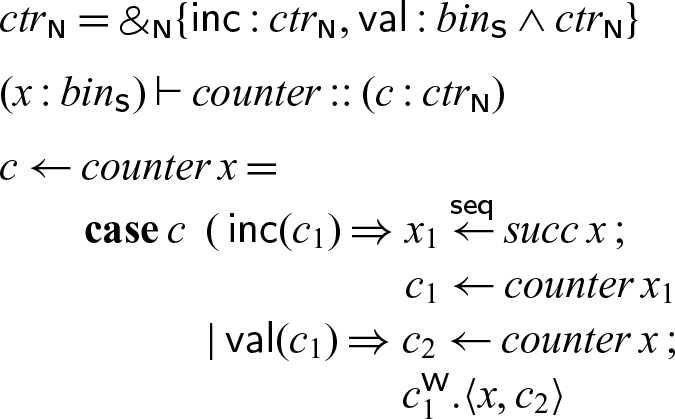
10 Conclusion
We have presented a concurrent shared-memory semantics based on a semi-axiomatic (DeYoung et al. Reference DeYoung, Pfenning and Pruiksma2020) presentation of adjoint logic (Reed Reference Reed2009; Licata & Shulman Reference Licata and Shulman2016; Licata et al. Reference Licata, Shulman, Riley and Miller2017; Pruiksma & Pfenning Reference Pruiksma, Pfenning, Martins and Orchard2019), for which we have usual variants of progress and preservation, as well as confluence. We then demonstrate that by adding a limited form of atomic writes, we can model sequential computation. Taking advantage of this, we reconstruct several patterns that provide limited access to concurrency in a sequential language, such as fork/join, futures, and monadic concurrency in the style of SILL. The uniform nature of these reconstructions means that they are all mutually compatible, and so we can freely work with any set of these concurrency primitives within the same language. Moreover, taking advantage of the adjoint nature of the language, we can have multiple modes, each with different features — for instance, one mode where computation is purely sequential, another with futures, and yet another with fork/join. The separation between these modes means that we can reason about programs at each mode separately — not needing to think about concurrency at the purely sequential mode, for example. Building on this, an actual implementation of this language could make optimizations based on the restrictions at each mode, not needing to worry about the full range of features that may exist at other modes. Seax therefore allows us to get many of the benefits of working in a restricted language (at a specific mode), without the drawbacks of only having specific tools to work with (since we can weaken those restrictions or place other restrictions at different modes).
There are several potential directions that future work in this space could take. In our reconstruction of futures, we incidentally also provide a definition of linear futures, which have been used in designing pipelines (Blelloch & Reid-Miller Reference Blelloch and Reid-Miller1999), but to our knowledge have not been examined formally or implemented. One item of future work, then, would be to further explore linear futures, now aided by a formal definition which is also amenable to implementation. We also believe that it would be interesting to explore an implementation of our language as a whole and to investigate what other concurrency patterns arise naturally when working in it. Another item of future work is to make more precise the correctness of the encodings we describe in Sections 6, 8 and 9. For instance, for functions, we can prove beta reduction admissible already, but for the other encodings, we lack similar results, as this kind of functional correctness result appears to require a better notion of equivalence for Seax processes, allowing us to compare terms in the languages augmented with additional constructs to terms in the base language that use encodings in place of those additional constructs. Additionally, the stratification of the language into layers connected with adjoint operators strongly suggests that some properties of a language instance as a whole can be obtained modularly from properties of the sublanguages at each mode. Although based on different primitives, research on monads and comonads to capture effects and coeffects, respectively (Curien et al. Reference Curien, Fiore and Munch-Maccagnoni2016; Gaboardi et al. Reference Gaboardi, ya Katsumata, Orchard, Breuvart and Uustalu2016), also points in this direction. In particular, we would like to explore a modular theory of (observational) equivalence using this approach. Some work on observational equivalence in a substructural setting already exists (Kavanagh Reference Kavanagh2020), but works in a message-passing setting and does not seem to translate directly to the shared-memory setting of Seax.
Conflicts of Interest
None.
Acknowledgments
This material is based upon work supported by the National Science Foundation under Grant No. 1718267.
1 Typed futures
The futures that we discuss in Section 7 behave much like Halstead’s original futures in Multilisp Halstead (Reference Halstead1985), which, rather than being distinguished at the type level, are purely operational. One side effect of this is that while we can explicitly synchronize these futures, we can also make use of implicit synchronization, where accessing the value of the future blocks until it has been computed, without the need for a touch construct.
Here, we will look at a different encoding of futures, which distinguishes futures at the type level, as they have often been presented since. As in Section 6, we will work with a single mode m, in which we will only allow sequential cuts, and which may have any set $\sigma(m)$
of structural properties. To the base language, we add the following new types and process terms for futures:
$\sigma(m)$
of structural properties. To the base language, we add the following new types and process terms for futures:
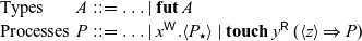 \begin{equation*} \begin{array}{llcl} \mbox{Types} & A & ::= & \ldots \mid \mathbf{fut}\, A \\ \mbox{Processes} & P & ::= & \ldots \mid x^{{\mathchoice{\textsf{W}}{\textsf{W}}{\scriptscriptstyle\textsf{W}}{\scriptscriptstyle\textsf{W}}}}.\langle P_\star \rangle \mid \mathbf{touch}\, y^{{\mathchoice{\textsf{R}}{\textsf{R}}{\scriptscriptstyle\textsf{R}}{\scriptscriptstyle\textsf{R}}}}\, (\langle z\rangle \Rightarrow P) \end{array}\end{equation*}
We type these new constructs as:
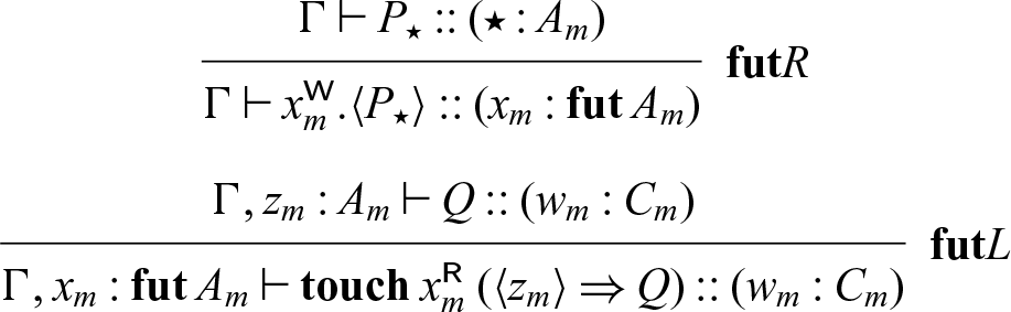
We then reconstruct this in Seax by defining
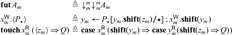 \begin{equation*} \begin{array}{lcl} \mathbf{fut}\, A_m & \triangleq & {\downarrow}^m_m {\downarrow}^m_m A_m \\[1ex] x_m^{{\mathchoice{\textsf{W}}{\textsf{W}}{\scriptscriptstyle\textsf{W}}{\scriptscriptstyle\textsf{W}}}}.\langle P_\star \rangle & \triangleq & y_m \leftarrow P_\star[y_m.\mathbf{shift}(z_m) // \star] \mathrel{;} x_m^{{\mathchoice{\textsf{W}}{\textsf{W}}{\scriptscriptstyle\textsf{W}}{\scriptscriptstyle\textsf{W}}}}.\mathbf{shift}(y_m) \\ \mathbf{touch}\, x_m^{{\mathchoice{\textsf{R}}{\textsf{R}}{\scriptscriptstyle\textsf{R}}{\scriptscriptstyle\textsf{R}}}}\, (\langle z_m\rangle \Rightarrow Q) & \triangleq & \mathbf{case}\, x_m^{{\mathchoice{\textsf{R}}{\textsf{R}}{\scriptscriptstyle\textsf{R}}{\scriptscriptstyle\textsf{R}}}}\, (\mathbf{shift}(y_m) \Rightarrow \mathbf{case}\, y_m^{{\mathchoice{\textsf{R}}{\textsf{R}}{\scriptscriptstyle\textsf{R}}{\scriptscriptstyle\textsf{R}}}} (\mathbf{shift}(z_m) \Rightarrow Q)) \\ \end{array}\end{equation*}
This is not the only possible reconstruction, Footnote 8 but we use it because it is the simplest one that we have found. The first property to verify is that these definitions are type-correct:
Theorem 9 If we expand all new constructs using $\triangleq$
, then the rules
$\triangleq$
, then the rules ${\mathbf{fut} L}$
and
${\mathbf{fut} L}$
and ${\mathbf{fut} R}$
are admissible.
${\mathbf{fut} R}$
are admissible.
Proof. By examining typing derivations for these processes, we see that these rules can be derived as follows:
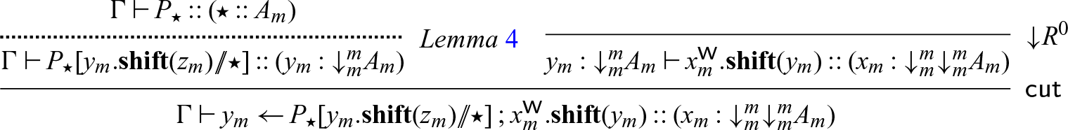
Note that we omit mode conditions on cut because within a single mode m, they are necessarily satisfied. $\square$
Now, we examine the computational behavior of these terms to demonstrate that they behave as futures. The type ${\downarrow}^m_m A_m$
, much like in Section 5 where we used it to model sequentiality, adds an extra synchronization point. Here, we shift twice, giving
${\downarrow}^m_m A_m$
, much like in Section 5 where we used it to model sequentiality, adds an extra synchronization point. Here, we shift twice, giving ${\downarrow}^m_m {\downarrow}^m_m A_m$
, to introduce two synchronization points. The first is that enforced by our restriction to only allow sequential cuts in this language (outside of futures), while the second will become the
${\downarrow}^m_m {\downarrow}^m_m A_m$
, to introduce two synchronization points. The first is that enforced by our restriction to only allow sequential cuts in this language (outside of futures), while the second will become the $\mathbf{touch}$
construct. We will see both of these when we examine each process term.
$\mathbf{touch}$
construct. We will see both of these when we examine each process term.
We begin by examining the constructor for futures. Intuitively, when creating a future, we would like to spawn a new thread to evaluate $P_\star$
with new destination
$P_\star$
with new destination $z_m$
, and immediately write the promise of
$z_m$
, and immediately write the promise of $z_m$
(represented by a hypothetical new value
$z_m$
(represented by a hypothetical new value $\langle z_m \rangle$
) into
$\langle z_m \rangle$
) into $x_m$
, so that any process waiting on
$x_m$
, so that any process waiting on $x_m$
can immediately proceed. The term
$x_m$
can immediately proceed. The term
 \begin{equation*}x_m^{{\mathchoice{\textsf{W}}{\textsf{W}}{\scriptscriptstyle\textsf{W}}{\scriptscriptstyle\textsf{W}}}}.\langle P_\star \rangle\quad \triangleq \quad y_m^{{\mathchoice{\textsf{W}}{\textsf{W}}{\scriptscriptstyle\textsf{W}}{\scriptscriptstyle\textsf{W}}}} \leftarrow P_\star[y_m.\mathbf{shift}(z_m) // \star] \mathrel{;} x_m^{{\mathchoice{\textsf{W}}{\textsf{W}}{\scriptscriptstyle\textsf{W}}{\scriptscriptstyle\textsf{W}}}}.\mathbf{shift}(y_m)\end{equation*}
behaves almost exactly as expected. Rather than spawning $P_\star$
with destination
$P_\star$
with destination $z_m$
, we spawn
$z_m$
, we spawn $P_\star[y_m.\mathbf{shift}(z_m) // \star]$
, which will write the result of
$P_\star[y_m.\mathbf{shift}(z_m) // \star]$
, which will write the result of $P_\star$
to
$P_\star$
to $z_m$
, and a synchronizing shift to
$z_m$
, and a synchronizing shift to $y_m$
. Concurrently, we write the value
$y_m$
. Concurrently, we write the value $\mathbf{shift}(y_m)$
to
$\mathbf{shift}(y_m)$
to $x_m$
, allowing the client of
$x_m$
, allowing the client of $x_m$
to resume execution, even if
$x_m$
to resume execution, even if $x_m$
was created by a sequential cut. This value
$x_m$
was created by a sequential cut. This value $\mathbf{shift}(y_m)$
is the first half of the promise
$\mathbf{shift}(y_m)$
is the first half of the promise $\langle z_m \rangle$
, and the second half,
$\langle z_m \rangle$
, and the second half, $\mathbf{shift}(z_m)$
, will be written to
$\mathbf{shift}(z_m)$
, will be written to $y_m$
when P finishes executing.
$y_m$
when P finishes executing.
If, while P continues to execute, we touch $x_m$
, we would expect to block until the promise
$x_m$
, we would expect to block until the promise $\langle z_m \rangle$
has been fulfilled by P having written to
$\langle z_m \rangle$
has been fulfilled by P having written to $z_m$
. Again, we see exactly this behavior from the term
$z_m$
. Again, we see exactly this behavior from the term
 \begin{equation*}\mathbf{touch}\, x_m^{{\mathchoice{\textsf{R}}{\textsf{R}}{\scriptscriptstyle\textsf{R}}{\scriptscriptstyle\textsf{R}}}}\, (\langle z_m\rangle \Rightarrow Q)\quad \triangleq \quad\mathbf{case}\, x_m^{{\mathchoice{\textsf{R}}{\textsf{R}}{\scriptscriptstyle\textsf{R}}{\scriptscriptstyle\textsf{R}}}}\, (\mathbf{shift}(y_m) \Rightarrow \mathbf{case}\, y_m^{{\mathchoice{\textsf{R}}{\textsf{R}}{\scriptscriptstyle\textsf{R}}{\scriptscriptstyle\textsf{R}}}} (\mathbf{shift}(z_m) \Rightarrow Q)).\end{equation*}
This process will successfully read $\mathbf{shift}(y_m)$
from
$\mathbf{shift}(y_m)$
from $x_m$
, but will block trying to read from
$x_m$
, but will block trying to read from $y_m$
until
$y_m$
until $y_m$
is written to. Since
$y_m$
is written to. Since $z_m$
and
$z_m$
and $y_m$
are written to at the same time, we block until
$y_m$
are written to at the same time, we block until $z_m$
is written to, at which point the promise is fulfilled. Once a result W has been written to
$z_m$
is written to, at which point the promise is fulfilled. Once a result W has been written to $z_m$
and (simultaneously)
$z_m$
and (simultaneously) $\mathbf{shift}(z_m)$
has been written to
$\mathbf{shift}(z_m)$
has been written to $y_m$
, this process can continue, reading both
$y_m$
, this process can continue, reading both $y_m$
and
$y_m$
and $z_m$
, and continuing as Q. Again, this is the behavior we expect a touch construct to have.
$z_m$
, and continuing as Q. Again, this is the behavior we expect a touch construct to have.
This approach does effectively model a form of typed future, which ensures that all synchronization is explicit, but comes at the cost of overhead from the additional shifts. Both this and the simpler futures that we describe in Section 7 have their uses, but we believe that the futures native to Seax are more intuitive in general.
2 Proofs of type correctness
In Sections 6, 8 and 9, we present type-correctness theorems for our reconstructions of various concurrency primitives, but omit the details of the proofs. Here, we present those details.
Functions. We derive the typing rules as follows, making use of Lemma 5 to use the admissible $\textsf{seqcut}$
rule. We omit the conditions on modes for cut, as we only have one mode:
$\textsf{seqcut}$
rule. We omit the conditions on modes for cut, as we only have one mode:
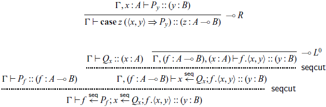
Fork/Join. Due to the length of the process term that defines $z.\langle P_\star \mid Q_\star \rangle$
, we elide portions of it throughout the derivation below, and we will write P’ for
$z.\langle P_\star \mid Q_\star \rangle$
, we elide portions of it throughout the derivation below, and we will write P’ for $P_\star[x'.\mathbf{shift}(x) // \star]$
, and similarly Q’ for
$P_\star[x'.\mathbf{shift}(x) // \star]$
, and similarly Q’ for $Q_\star[y'.\mathbf{shift}(y) // \star]$
. With these abbreviations, we have the following derivation for the
$Q_\star[y'.\mathbf{shift}(y) // \star]$
. With these abbreviations, we have the following derivation for the $\Vert R$
rule, where the dashed inferences are made via Lemma 4.
$\Vert R$
rule, where the dashed inferences are made via Lemma 4.
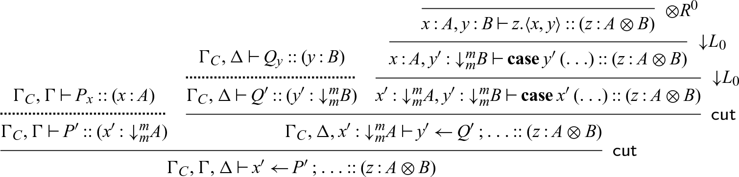
The left rule is much more straightforward, since this encoding makes the writer of the pair rather than the reader responsible for synchronization.
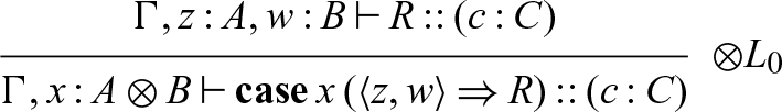
Monadic Concurrency. We first construct the typing rules for $\{\cdot\}$
, which are straightforward:
$\{\cdot\}$
, which are straightforward:
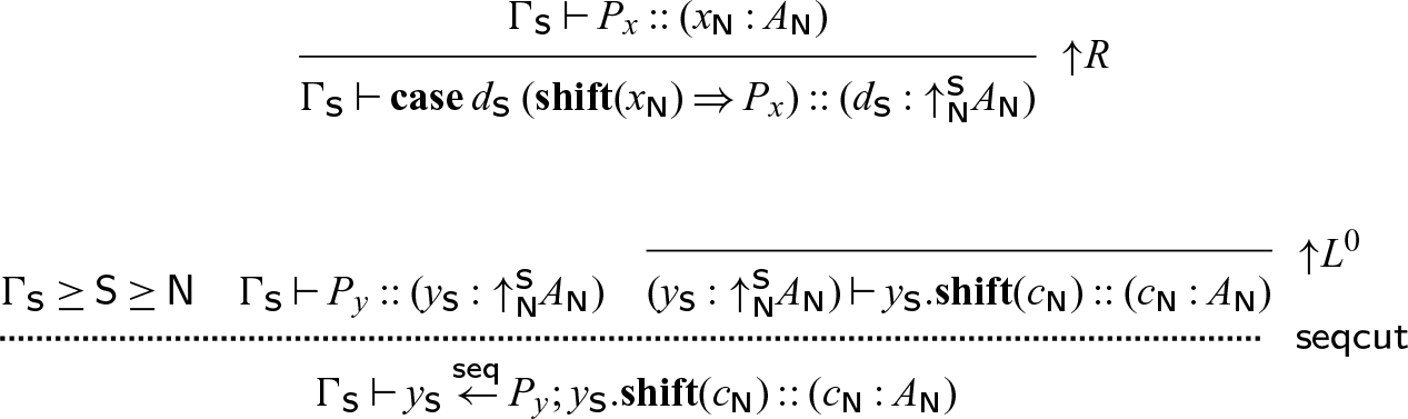
We then construct the typing rules for $\land$
:
$\land$
:
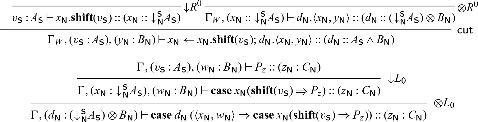
Note that unlike the rules for $\{\cdot\}$
or for many of the constructs in previous sections, those for
$\{\cdot\}$
or for many of the constructs in previous sections, those for $\land$
are not only admissible — they are derivable.
$\land$
are not only admissible — they are derivable.


 Open access
Discussions
No Discussions have been published for this article.