2 Sneak preview

To illustrate the trinity of printer, parser, and proof combinators, we use the type of bushes, defined below, as a running example. (A similar datatype is required later for Huffman encoding, so our efforts are not wasted.)

For each type ${\textit{A}}$ whose elements we wish to serialise, we define a module called ${\textit{Codec-A}}$ .

Printing combinators. A bit string or code is generated using ${\epsilon}$ , ${\_\mathord{\cdot}\_}$ , , and ${\mathtt{I}}$ . The encoder for bushes employs all four combinators.

An encoder for elements of type ${\textit{A}}$ is typically defined by structural recursion on ${\textit{A}}$ , encode is no exception. Each constructor is encoded by a suitable number of bits followed by the encodings of its arguments, if any. For the example at hand, a single bit suffices. In general, we require $\lceil\log_2 n\rceil$ bits if the datatype comprises n constructors. (Of course, we may also apply Huffman’s idea to the encoding of constructors using variable-length instead of fixed-length bit codes.) Concatenation ${\_\mathord{\cdot}\_}$ is associative with ${\epsilon}$ as its neutral element, so the trailing ${\epsilon}$ s seem a bit odd—odd, but convenient as we shall see shortly.

Parsing combinators. Decoders can be most conveniently defined using -notation as the type of decoders has the structure of a monad.

The decoder performs a case analysis on the first bit of the implicit input bit string, and then, it decodes the arguments, if any. In the best, or, worst tradition of Haskell, is defined recursively. Unfortunately, Agda is not able to establish its termination. All is safe, however: the case analysis consumes a bit, so both recursive calls process strictly smaller bit strings. The pragma preceding the definition communicates our findings to Agda.

We have come across a well-known problem in parsing: a recursive-descent parser may fail to terminate if the underlying grammar is left-recursive. Consequently, when decoders are defined recursively, we need to make sure that each recursive call is guarded by at least one case combinator. Are we happy to accept the potential threat of non-termination? No! We should be able to do better than that. And indeed, the parser library features a grown-up version of case analysis that allows for safe recursive calls.

The combinator can be seen as a recursion principle for bit strings; it passes the ability to issue recursive calls to each branch. All is well now: Agda happily accepts the definition; decode terminates on all inputs.

Proof combinators. We have created two independent artefacts: an encoder and a decoder. It remains to relate the two: we require that decoding an encoded value gives back the original value. To capture this property, we make use of a ternary relation, relating bit strings, values, and decoders: ${\textit{s}\mkern6mu\mathord{\langle}\mkern6mu\textit{a}\mkern6mu\mathord{\rangle}\mkern6mu\textit{p}}$ holds iff ${\textit{p}}$ “applied” to s returns a. The correctness criterion then reads

(2.1)

The library offers six proof combinators for discharging the proof obligation, presented as proof rules below. (Each rule is actually the type of the proof combinator—“propositions as types” at work.)

The axiom relates the unit of the monoid to the “unit” of the monad; the rule relates the multiplication of the monoid to the “multiplication” of the monad.

The case parser consumes a bit and then acts as one of the branches. The recursive variant additionally passes “itself” to the branch.

The proof of correctness then typically proceeds by structural recursion on the type of the to-be-encoded values, here the type of bushes.

Two remarks are in order.

The definition of encode features trailing ${\epsilon}$ s so that all three artefacts, printers, parsers, and proofs, exhibit exactly the same structure. Any deviation incurs additional proof effort as monoid and monad laws do not hold on the nose, for example, ${\textit{s}\mkern6mu{\cdot}\mkern6mu\epsilon}$ is not definitionally equal to s, only propositionally.

Each proof combinator takes a couple of implicit arguments—the variables appearing in the proof rules. Agda happily infers these arguments from the data provided, with one exception: the needs p and q as explicit arguments. Consequently, the proof is actually more verbose.

On the positive side, the additional arguments show very clearly how the parsing process proceeds, creating a in two steps.

Codecs. For convenience, the three entities are wrapped up in a record.

For each serialisable type ${\textit{A}\mkern6mu\mathord{:}\mkern6mu\textit{Set}}$ we define a codec . You may want to view ${\textit{Codec}}$ as a property of a type, or as a type class and ${\textit{Codec}\mkern6mu\textit{A}}$ as an instance dictionary.

The definition makes use of a nifty Agda feature: the syntax constructs a record of type R, using suitable components from the module M.

For reference, Figure 1 shows a codec for a second example, the naturals. This completes the description of the interface. Next, we turn to the implementation, starting with parsing combinators as their design dictates everything else.

Fig. 1.

A codec for natural numbers.

3 Parsing combinators

The goal is clear: our parsing combinators should come with a termination guarantee as Agda is not able to establish termination of recursively defined decoders. To understand the cure, let us delve a bit deeper into the problem.

First, we introduce the type of bit strings. A bit string is either empty, written , or a binary digit, or , followed by a bit string.

The problem. A decoder is a deterministic parser, combining state, bit strings of type Bits, and partiality, the Maybe monad (see Appendix 1). Not using any special combinators, a decoder for bushes can be implemented as follows.

Observe how the state, the bit string, is threaded through the program. Putting the termination spectacles on, the first recursive call is benign as bs is an immediate substring of bs. The second recursive call is, however, problematic as decode is applied to the string returned from the first call. Agda has no clue that is actually smaller than bs.

The recursion pattern is an instance of course-of-values recursion or strong recursion where a function recurses on all smaller values, for example, where ${\textit{f}\mkern6mu(\textit{n}\mkern6mu\mathord{+}\mkern6mu1)}$ is computed from ${\textit{f}\mkern6mu(0)}$ , $\ldots$ , ${\textit{f}\mkern6mu(\textit{n})}$ . Perhaps a short detour is worthwhile to remind ourselves of this induction and recursion principle.

Detour: strong versus structural recursion. Say, is a property of the naturals, established by strong induction. Strong induction can be reduced to structural induction by proving a stronger property: ${\textit{Q}\mkern6mu\textit{m}\mkern6mu\mathrel{=}\mkern6mu\textit{P}\mkern6mu0\mkern6mu\wedge\mkern6mu\cdots\mkern6mu\wedge\mkern6mu\textit{P}\mkern6mu\textit{m}}$ , or, avoiding ellipsis ${\textit{Q}\mkern6mu\textit{m}\mkern6mu\mathrel{=}\mkern6mu\forall\mkern6mu\textit{n}\mkern6mu\mathord{\to}\mkern6mu\textit{m}\mkern6mu\succcurlyeq\mkern6mu\textit{n}\mkern6mu\mathord{\to}\mkern6mu\textit{P}\mkern6mu\textit{n}}$ .

Say, is a function from the naturals, defined by strong recursion. Strong recursion can be reduced to structural recursion by defining a stronger function: ${\textit{g}\mkern6mu\textit{m}\mkern6mu\mathord{:}\mkern6mu\forall\mkern6mu\textit{n}\mkern6mu\mathord{\to}\mkern6mu\textit{m}\mkern6mu\succcurlyeq\mkern6mu\textit{n}\mkern6mu\mathord{\to}\mkern6mu\textit{A}}$ . Consider as an example,

This is the simplest, non-trivial example I could think of: ${\textit{f}\mkern6mu(\textit{n}\mkern6mu\mathord{+}\mkern6mu1)}$ is given by the sum of all smaller values: ${\textit{f}\mkern6mu(0)\mkern6mu\mathord{+}\mkern6mu\cdots\mkern6mu\mathord{+}\mkern6mu\textit{f}\mkern6mu(\textit{n})}$ . (Do you see what f computes?) Its stronger counterpart is given by

If we remove the first and the third argument of g and the second argument of the helper function sg, we get back the original definition: ${\textit{g}\mkern6mu\textit{m}\mkern6mu\textit{n}\mkern6mu\textit{m}\succcurlyeq\textit{n}\mkern6mu\equiv\mkern6mu\textit{f}\mkern6mu\textit{n}}$ for all natural numbers m and n with In particular, f can be reduced to its counterpart: ${\textit{f}\mkern6mu\textit{n}\mkern6mu\mathrel{=}\mkern6mu\textit{g}\mkern6mu\textit{n}\mkern6mu\textit{n}\mkern6mu\mathord{\succcurlyeq}\!{-reflexive}}.$ Observe that g is defined by structural recursion on the first argument; the helper function maintains the invariant that the “actual” argument i is at most m.

The solution. Returning to our application, we would like to define decoders by strong induction over the length of bit strings. As a preparatory step, we replace the original definition of Bits by an indexed type that records the length.

Compared to the number-theoretic example above, there is one further complication: we need to relate the length of the residual bit string returned by a parser to the length of its input. Exact numbers are not called for; it suffices to know that the length of the output is at most the length of the input. To this end, we introduce ${\textit{Bits}\mathord{\preccurlyeq}\mkern6mu\textit{n}}$ , the type of bit strings of length below a given upper bound n.

The record features three fields, the first of which is hidden, indicated by curly braces. If the decoder transmogrifies, say, ${\textit{bs}\mkern6mu\mathord{:}\mkern6mu\textit{Bits}\mkern6mu\textit{i}}$ to with ${\textit{i}\mathord{\succcurlyeq}\textit{j}\mkern6mu\mathord{:}\mkern6mu\textit{i}\mkern6mu\succcurlyeq\mkern6mu\textit{j}}$ , then the residual output of type ${\textit{Bits}\mathord{\preccurlyeq}\mkern6mu\textit{i}}$ is given by .

Finally, we have all the gadgets in place, to define a decoder that is approved by Agda’s termination checker. As to be expected, its type is more involved. In a sense, decode says: I can decode a bit string of size i, but I am happy to accept any bit string of smaller size; I promise to return a bush and a string, the length of which is at most the size of the string given to me.

Voilà, decode is defined by structural recursion on the natural number i. To reduce clutter, the actual size of the bit string is passed implicitly. In the recursive case, we have ${\textit{bs}\mkern6mu\mathord{:}\mkern6mu\textit{Bits}\mkern6mu\textit{j}}$ , and with ${\textit{j}\mkern6mu\succcurlyeq\mkern6mu\textit{k}}$ and ${\textit{k}\mkern6mu\succcurlyeq\mkern6mu\textit{m}}$ . All that remains to be done is to hide the plumbing of state and proofs.

Hiding the plumbing. A decoder is a function from bit strings to an optional pair of things and bit strings, promising not to increase the length of the string.

Both ${\textit{IDecoder}\mkern6mu\textit{A}}$ and ${\textit{Bits}\mathord{\preccurlyeq}}$ are indexed by naturals numbers, and they are functions of type . But there is more to them, they are actually functors: ${\textit{IDecoder}\mkern6mu\textit{A}}$ is a covariant functor from the preorder ${({\mathbb{N},}\mkern6mu\succcurlyeq)}$ , viewed as a category, to the category of sets and total functions. Its action on arrows is defined

The function lower makes precise the idea that a decoder can be applied to any shorter bit string. By contrast, ${\textit{Bits}\mathord{\preccurlyeq}}$ is a contravariant functor: we may relax the upper bound.

Turning to the implementation of the monad operations, the definition of return is standard, except for the proof that the length is unchanged.

The implementation of monadic bind is more interesting.

The value a returned by p is passed to the continuation q. Since we wish to apply ${\textit{q}\mkern6mu\textit{a}}$ to the residual input , we need to lower its index. This move has a knock-on effect: the upper bound of q’s result is consequently too low and needs to be relaxed in a final step.

The case combinator dispatches on the first bit of the input bit string. It fails if the input is exhausted. This is the single source of undefinedness—the correctness proofs guarantee that this failure never happens for “legal” inputs.

Again, we first lower the index and then adjust the upper bound of the result. The proof records the fact that bs is one element shorter compared to or .

It is time to bring in the harvest! The implementation of recursive case analysis merits careful study.

The recursor is defined by structural induction on its first argument. The entire set-up—the use of indexed types, keeping track of bounds—serves the sole purpose of enabling this definition. Observe that the type of branches involves a local quantifier: the branches work for any index, in particular, they happily accept the recursive call at index ${\textit{i}\mkern6mu\mathord{-}\mkern6mu1}$ .

Ultimately, the four combinators enable the user to construct decoders that work for any index.

4 Pretty-printing combinators

For reasons of efficiency, encoders use John Hughes’ representation of lists (Hughes, Reference Hughes1986), specialised to bit strings.

Encoders are dual to decoders. While decoders promise not to increase the size of the bit string, encoders guarantee not to decrease its size. To capture this invariant, we need the dual of ${\textit{Bits}\mathord{\preccurlyeq}}$ , bit strings of size above a given bound:

Composition of functions and proofs then serves as concatenation with the identity as its neutral element.

The combinators and ${\mathtt{I}}$ increase the size by one.

As an amusing aside, the proof that Code is a monoid makes use of the fact that ${({\mathbb{N},}\mkern6mu\preccurlyeq)}$ is a category: ${\mathord{\preccurlyeq}{-transitive}}$ is associative with ${\mathord{\preccurlyeq}{-reflexive}}$ as its neutral element.

5 Proof combinators

Decoders are partial functions. Given an arbitrary bit string, a decoder might fail, unexpectedly exhausting the input. The correctness criterion (2.1) guarantees that this does not happen if a decoder is applied to an encoding. This guarantee is, in a sense, the sole purpose of the whole exercise. The ternary relation ${\_\mathord{\langle}\_\mathord{\rangle}\_}$ underlying (2.1) relates a code, an element, and a decoder.

The function code prepends some bits to bs; the decoder removes this prefix returning the value a and bs. This relation must hold for any upper bound i.

The implementation of the proof combinators is fairly straightforward. The code is, however, not too instructive, so we content ourselves with two illustrative examples. (The definition of the remaining combinators can be found in the accompanying material.)

The axiom $\epsilon$ -axiom holds definitionally: Agda can show its correctness solely by unfolding definitions, witnessed by the use of ${\mathord{\equiv}{-reflexive}\mkern6mu\mathord{:}\mkern6mu\textit{a}\mkern6mu\equiv\mkern6mu\textit{a}}$ .

To establish the ,

we apply the premise to the argument of ${\textit{relax}\mkern6mu{succ-n}\mathord{\succcurlyeq}{n}}$ .

Now that the core library is in place, we can finally deal with the motivating example, Huffman Encoding. Its implementation turns out to be a nice exercise in datatype-generic programming.

6 Application: Huffman encoding

Before diving into the mechanics of Huffman compression, let us state the guiding principles of the design: (1) we would like to seamlessly combine statistical compression with standard serialisers; (2) we aim to avoid irrelevant detail, such as: Is the code unambiguous? Does the alphabet contain at least two characters? Huffman encoding typically relies on a dictionary, mapping characters to codes; Huffman decoding makes use of a code tree. Does the dictionary contain a code for each to-be-encoded character? Is the code tree actually related to the dictionary? And so forth, and so forth … In other words, we are aiming for a clean, lean interface.

We proceed in three steps, defining a codec for a single character, for a sequence of characters, and for Huffman code trees.

6.1 Encoding and decoding characters

The central property of variable-length encodings is that no code is a prefix of any other code. This property is guaranteed by construction if a code tree is used instead of a code table. The code tree corresponding to Table (1.2) is depicted below.

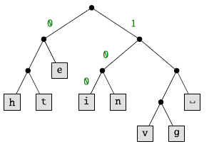
The character , for example, is encoded by . So, as a first requirement, we assume that a code tree is given to us. A code tree is either a singleton, written , or a binary node , where t and u are code trees (the bushes of Section 2 are code trees without codes).

The code tree above is represented by

Using this encoding, we can compress the text (1.1), but not genius, as neither u nor s have an encoding. This motivates the second requirement: we need evidence that the to-be-compressed character is contained in the code tree.

The evidence can be seen as a path into the tree. For example,

certifies that is in the code tree code: starting at the root, it can be found going to the right and then twice to the left.

Perhaps surprisingly, no further requirements are necessary: our Huffman compressor takes a pair such as , consisting of a single character and a proof that this character is contained in the code tree. Observe that the type of the second component depends on the value of the first component (in the “propositions as types” paradigm a proposition such as is a type). In other words, the data are a dependent pair, an element of a $\Sigma$ type (Alphabet is an implicit type argument, indicated by curly braces).

Elements of the type ${\textit{In}\mkern6mu\textit{t}}$ can be seen as self-certifying data: data that can be readily serialised.

The encoder turns the evidence, the path into the code tree, into a bit string, ignoring both the code tree and the character!

The decoder has to resurrect the path. For this to work out, the code tree is required.

The bits steer the search, the decoder stops if a leaf is reached. Note that we do not use the recursive case combinator; decode is recursively defined by induction on the structure of the code tree.

The proof of correctness replicates the structure of encoder and decoder.

For brevity, we henceforth omit the correctness proof—in all the examples, it can be mechanically derived from the encoder.

Provided with a code tree, the Huffman serialiser happily deals with a single self-certified character.

Before we tackle the encoding of strings, it is worthwhile recording what we do not need to assume. We do not require that the character has a unique code; it may appear multiple times in the code tree. (Perhaps, bit strings are used to exchange secret messages. Using different codes for the same letter may slightly improve security.) Neither do we require that each element of Alphabet appears in the code tree. (If the underlying alphabet is large—the current Unicode standard defines 144,697 characters—then a text will rarely include each character.) Finally, the compressor works for arbitrary code trees, including trees that consist of a single leaf. These extreme cases feature a fantastic compression rate as no bits are required. (Usually some care must be exercised to avoid sending the decoder into an infinite loop. The decoder presented in Stump (Reference Stump2016) exercises this care but fails with an error message instead!)

6.2 Encoding and decoding sequences

Let us be slightly more ambitious by not only considering strings, sequences of characters, but sequences of arbitrary encodable values. There are at least two options for defining a suitable container type; we discuss each in turn.

The obvious choice is to use standard lists, given by the definition below.

The type features two data constructors; to distinguish between empty and non-empty lists we need one bit.

The codec for List takes a codec for A to a codec for ${\textit{List}\mkern6mu\textit{A}}$ .

You may recognise the type pattern if you are familiar with Haskell’s type classes or with datatype-generic programming.

Unfortunately, if we compose the list encoder with our Huffman encoder, then the compression factor suffers, as the code for each character is effectively prolonged by one bit. By contrast, the standard Huffman compressor, which operates on strings, simply concatenates the character codes; the decompressor keeps decoding until the input is exhausted. Alas, this approach is in conflict with our modularity requirements: such a codec cannot be used as a component of other codecs. (Imagine compressing tree-structured data such as HTML, using the statistical compressor for leaves, paragraphs of text.)

We can save the additional bit per list item if we keep track of the total number of items. In other words, we may want to use a vector, a length-indexed list, instead of a standard list.

The constructor names are chosen to reflect that a vector is really a nested pair. Like the type of lists, Vector features two data constructors. However, only one of these is available for each given length—there is only one shape of vector. So the good news is that no bits are required to encode the constructors.

The encoder and the decoder are driven by the length argument, which is passed implicitly to encode and explicitly to decode.

Of course, for our application at hand we need to store the length alongside the vector, another case for dependent pairs:

Inspecting the type on the right-hand side, we note that we already have a codec for naturals and vectors, so we are left with defining a codec for $\Sigma$ -types.

Encoding dependent pairs is not too hard, the main challenge is to get the type signature right. A dependent pair consists of a field ${\textit{a}\mkern6mu\mathord{:}\mkern6mu\textit{A}}$ and a field ${\textit{b}\mkern6mu\mathord{:}\mkern6mu\textit{B}\mkern6mu\textit{a}}$ . This dependency is reflected in the types of the codecs:

The implementation is identical to a codec for standard pairs, except that the first field is passed to the codec for the second field.

Assembling the various bits and pieces,

is a space-efficient codec for sequences. Well, not quite. A moment’s reflection reveals that we have not gained anything: and produce bit strings of exactly the same length. (This tells you something about the relation between lists, naturals, and vectors.) We have chosen to represent naturals in unary. Consequently, the vector length n is encoded by a bit string of length $n + 1$ . That said, a cure is readily at hand: we simply switch to a binary or ternary representation.

We seize the opportunity and define a general codec for representation changers. Given an isomorphism ${\textit{A}\mkern6mu\cong\mkern6mu\textit{B}}$ , we can turn a codec for A into a codec for B. The functions witnessing the isomorphism are called and .

We chose to replace unary numbers by ternary ^{Footnote 1} numbers, obtaining the final implementation of the encoder for sequences:

Our library is taking shape. s

We can, for instance, confirm that the introductory example (1.1) is compressed to 59 bits—we assume below that ${\textit{text}\mkern6mu\mathord{:}\mkern6mu\textit{Vector}\mkern6mu(\textit{In}\mkern6mu\textit{code})\mkern6mu20}$ is provided from somewhere.

Additional 8 bits are needed to store the length.

6.3 Encoding and decoding code trees

All that remains to be done is to define a codec for Huffman trees. The type of code trees is a standard container type, so this is a routine exercise by now—the codec for bushes, see Section 2, serves nicely as a blueprint.

A Huffman compressor stores the code tree alongside the encoded text. Since the encoding depends on the tree this is another example of a dependent pair—actually, quite a nice one. (Once you start looking closely, you notice that dependent pairs are everywhere.)

An element of the type is a dependent pair consisting of a code tree and a length-encoded list of self-certifying characters. The corresponding codec is obtained simply by changing the font.

Voilà, again. The compositional approach shows its strengths. In particular, it is easy to change aspects. For example, to compress a list of lists of characters, we simply replace the inner codec by .