


1 Introduction
Primitive recursion has a solid foundation in a variety of different fields. In the categorical setting, it can be seen in the structures of algebras. In the logical setting, it corresponds to proofs by induction. And in the computational setting, it can be phrased in terms of languages and type theories with terminating loops, like Gödel’s System (Gödel, Reference Gödel1980). The latter viewpoint of computation reveals a fine-grained lens with which we can study the subtle impact of the primitive combinators that capture different forms of recursion. For example, the recursive combinators given by Mendler (Reference Mendler1987, Reference Mendler1988) yield a computational complexity for certain programs when compared to encodings in System (Böhm & Berarducci, Reference Böhm and Berarducci1985; Girard et al., Reference Girard, Lafont and Taylor1989). Recursive combinators have desirable properties—like the fact that they always terminate—which make them useful for the design of well-behaved programs (Meijer et al., Reference Meijer, Fokkinga and Paterson1991; Gibbons, Reference Gibbons2003), also for optimizations made possible by applying those properties and theorems (Malcolm, Reference Malcolm1990).
The current treatment of the dual of primitive recursion—primitive corecursion—is not so fortunate. Being the much less understood of the two, corecursion is usually only viewed in light of this duality. Consequently, corecursion tends to be relegated to a notion of coalgebras (Rutten, Reference Rutten2019), because only the language of category theory speaks clearly enough about their duality. This can be seen in the study of corecursion schemes, where coalgebraic “anamorphisms” (Meijer et al., Reference Meijer, Fokkinga and Paterson1991) and “apomorphisms” (Vos, Reference Vos1995; Vene & Uustalu, 1998) are the dual counterparts to algebraic “catamorphisms” (Meertens, Reference Meertens1987; Meijer et al., Reference Meijer, Fokkinga and Paterson1991; Hinze et al., 2013) and “paramorphisms” (Meertens, Reference Meertens1992). Yet the logical and computational status of corecursion is not so clear. For example, the introduction of stream objects is sometimes described as the “dual” to the elimination of natural numbers (Crole, Reference Crole2003; Sangiorgi, Reference Sangiorgi2011), but how is this so?
The goal of this paper is to provide a purely computational and logical foundation for primitive corecursion based on classical logic. Specifically, we will express different principles of corecursion in a small core calculus, analogous to the canonical computational presentation of recursion (Gödel, Reference Gödel1980). Much of the early pioneering work in this area was inspired directly by the duality inherent in (co)algebras and category theory (Hagino, 1987; Cockett & Spencer, Reference Cockett and Spencer1995). In contrast, we derive the symmetry between recursion and corecursion through the mechanics of programming language implementations, formalized in terms of an abstract machine. This symmetry is encapsulated by the syntactic and semantic duality (Downen et al., Reference Downen, Johnson-Freyd and Ariola2015) between data types—defined by the structure of objects—and codata types—defined by the behavior of objects.
We begin in Section 2 with a review of the formalization of primitive recursion in terms of a foundational calculus: System T (Gödel, Reference Gödel1980). We point out the impact of evaluation strategy on different primitive recursion combinators, namely the recursor and the iterator:
In call-by-value, the recursor is just as (in)efficient as the iterator.
In call-by-name, the recursor may end early; an asymptotic complexity improvement.
Section 3 presents an abstract machine for both call-by-value and call-by-name evaluation and unifies both into a single presentation (Ariola et al., 2009; Downen & Ariola, 2018b).The lower-level nature of the abstract machine explicitly expresses how the recursor of inductive types, like numbers, accumulates a continuation during evaluation, maintaining the progress of recursion. This is implicit in the operational model of System T. The machine is shown correct, in the sense that a well-typed program will always terminate and produce an observable value (Theorem 3.2), which in our case is a number.
Section 4 continues by extending the abstract machine with the primitive corecursor for streams. The novelty is that this machine is derived by applying syntactic duality, corresponding to de Morgan duality, to the machine with recursion on natural numbers, leading us to a classical corecursive combinator with multiple outputs modeled as multiple continuations. This corecursor is classical in the sense that it abstracts binds first-class continuations using control effects in a way that corresponds to multiple conclusions in classical logic (à la $\lambda\mu$
-calculus (Parigot, 1992) and the classical sequent calculus (Curien & Herbelin, 2000)). From de Morgan duality in the machine, we can see that the corecursor relies on a value accumulator; this is logically dual to the recursor’s return continuation. Like recursion versus iteration, in Section 5 we compare corecursion versus coiteration: corecursion can be more efficient than coiteration by letting corecursive processes stop early. Since corecursion is dual to recursion, and call-by-value is dual to call-by-name (Curien & Herbelin, 2000; Wadler, Reference Wadler2003), this improvement in algorithmic complexity is only seen in call-by-value corecursion. Namely:
$\lambda\mu$
-calculus (Parigot, 1992) and the classical sequent calculus (Curien & Herbelin, 2000)). From de Morgan duality in the machine, we can see that the corecursor relies on a value accumulator; this is logically dual to the recursor’s return continuation. Like recursion versus iteration, in Section 5 we compare corecursion versus coiteration: corecursion can be more efficient than coiteration by letting corecursive processes stop early. Since corecursion is dual to recursion, and call-by-value is dual to call-by-name (Curien & Herbelin, 2000; Wadler, Reference Wadler2003), this improvement in algorithmic complexity is only seen in call-by-value corecursion. Namely:
In call-by-name, the corecursor is just as (in)efficient as the coiterator.
In call-by-value, the corecursor may end early; an asymptotic complexity improvement.
Yet, even though we have added infinite streams, we don’t want to ruin System T’s desirable properties. So in Section 6, we give an interpretation of the type system which extends previous models of finite types (Downen et al., Reference Downen, Johnson-Freyd and Ariola2020, Reference Downen, Ariola and Ghilezan2019) with the (co)recursive types of numbers and streams. The novel key step in reasoning about (co)recursive types is in reconciling two well-known fixed point constructions—Kleene’s and Knaster-Tarski’s—which is non-trivial for classical programs with control effects. This lets us show that, even with infinite streams, our abstract machine is terminating and type safe (Theorem 6.14).
In summary, we make the following contributions to the understanding of (co)recursion in programs:
We present a typed uniform abstract machine, with both call-by-name and call-by-value instances, that can represent functional programs that operate on both an inductive type (Figs. 4 and 6) and a coinductive type (Figs. 7 to 8).
In the context of the abstract machine (Section 4.2), we show how the primitive corecursion combinator for a coinductive type can be formally derived from the usual recursor of an inductive type using the notion of de Morgan duality in classical logic. This derivation is made possible by a computational interpretation of involutive duality inherent to classical logic (Fig. 9 and Theorem 4.2).
We informally analyze the impact of call-by-value versus call-by-name evaluation on the algorithmic complexity of different primitive combinators for (co)inductive types. Dual to the fact that primitive recursion is more efficient than iteration (only) in call-name (Section 3.5), we show that classical corecursion is more efficient than intuitionistic coiteration (only) in call-by-value (Section 5).
The combination of primitive recursion and corecursion is shown to be type safe and terminating in the abstract machine (Theorem 6.14), even though it can express infinite streams that do not end. This is proved using an extension of bi-orthogonal logical relations built on a semantic notion of subtyping (Section 6).
Proofs to all theorems that follow are given in the appendix. For further examples of how to apply classical corecursion in real-world programming languages, and for an illustration of how classicality adds expressive power to corecursion, see the companion paper (Downen & Ariola, 2021).
2 Recursion on natural numbers: System T
We start with Gödel’s System T (Gödel, Reference Gödel1980), a core calculus which allows us to define functions by structural recursion. Its syntax is given in Fig. 1. It is a canonical extension of the simply typed $\lambda$
-calculus, whose focus is on functions of type
$\lambda$
-calculus, whose focus is on functions of type $A \to B$
, with ways to construct natural numbers of type
$A \to B$
, with ways to construct natural numbers of type $\operatorname{Nat}$
. The
$\operatorname{Nat}$
. The $\operatorname{Nat}$
type comes equipped with two constructors
$\operatorname{Nat}$
type comes equipped with two constructors $\operatorname{zero}$
and
$\operatorname{zero}$
and $\operatorname{succ}$
, and a built-in recursor, which we write as
$\operatorname{succ}$
, and a built-in recursor, which we write as $\operatorname{\mathbf{rec}} M \operatorname{\mathbf{as}}{} \{\operatorname{zero} \to N \mid \operatorname{succ} x \to y.N'\}$
. This
$\operatorname{\mathbf{rec}} M \operatorname{\mathbf{as}}{} \{\operatorname{zero} \to N \mid \operatorname{succ} x \to y.N'\}$
. This $\operatorname{\mathbf{rec}}$
-expression analyzes M to determine if it has the shape
$\operatorname{\mathbf{rec}}$
-expression analyzes M to determine if it has the shape $\operatorname{zero}$
or
$\operatorname{zero}$
or $\operatorname{succ} x$
, and the matching branch is returned. In addition to binding the predecessor of M to x in the
$\operatorname{succ} x$
, and the matching branch is returned. In addition to binding the predecessor of M to x in the $\operatorname{succ} x$
branch, the recursive result—calculated by replacing M with its predecessor x—is bound to y.
$\operatorname{succ} x$
branch, the recursive result—calculated by replacing M with its predecessor x—is bound to y.
System T: $\lambda$
-calculus with numbers and recursion.
$\lambda$
-calculus with numbers and recursion.

The type system of System T is given in Fig. 2. The var, ${\to}I$
and
${\to}I$
and ${\to}E$
typing rules are from the simply typed
${\to}E$
typing rules are from the simply typed $\lambda$
-calculus. The two
$\lambda$
-calculus. The two ${\operatorname{Nat}}I$
introduction rules give the types of the constructors of
${\operatorname{Nat}}I$
introduction rules give the types of the constructors of $\operatorname{Nat}$
, and the
$\operatorname{Nat}$
, and the ${\operatorname{Nat}}E$
elimination rule types the
${\operatorname{Nat}}E$
elimination rule types the $\operatorname{Nat}$
recursor.
$\operatorname{Nat}$
recursor.
Type system of System T.

System T’s call-by-name and call-by-value operational semantics are given in Fig. 3. Both of these evaluation strategies share operational rules of the same form, with $\beta_\to$
being the well-known
$\beta_\to$
being the well-known $\beta$
rule of the
$\beta$
rule of the $\lambda$
-calculus, and
$\lambda$
-calculus, and $\beta_{\operatorname{zero}}$
and
$\beta_{\operatorname{zero}}$
and $\beta_{\operatorname{succ}}$
defining recursion on the two
$\beta_{\operatorname{succ}}$
defining recursion on the two $\operatorname{Nat}$
constructors. The only difference between call-by-value and call-by-name evaluation lies in their notion of values V (i.e., those terms which can be substituted for variables) and evaluation contexts (i.e., the location of the next reduction step to perform). Note that we take this notion seriously and never substitute a non-value for a variable. As such, the
$\operatorname{Nat}$
constructors. The only difference between call-by-value and call-by-name evaluation lies in their notion of values V (i.e., those terms which can be substituted for variables) and evaluation contexts (i.e., the location of the next reduction step to perform). Note that we take this notion seriously and never substitute a non-value for a variable. As such, the $\beta_{\operatorname{succ}}$
rule does not substitute the recursive computation
$\beta_{\operatorname{succ}}$
rule does not substitute the recursive computation $\operatorname{\mathbf{rec}} V \operatorname{\mathbf{as}} \ \{ \operatorname{zero} \to N \mid \operatorname{succ} x \to y. N' \}$
for y, since it might not be a value (in call-by-value). The next reduction step depends on the evaluation strategy. In call-by-name, this next step is indeed to substitute
$\operatorname{\mathbf{rec}} V \operatorname{\mathbf{as}} \ \{ \operatorname{zero} \to N \mid \operatorname{succ} x \to y. N' \}$
for y, since it might not be a value (in call-by-value). The next reduction step depends on the evaluation strategy. In call-by-name, this next step is indeed to substitute $\operatorname{\mathbf{rec}} V \operatorname{\mathbf{as}} \ \{ \operatorname{zero} \to N \mid \operatorname{succ} x \to y. N' \}$
for y, and so we have:
$\operatorname{\mathbf{rec}} V \operatorname{\mathbf{as}} \ \{ \operatorname{zero} \to N \mid \operatorname{succ} x \to y. N' \}$
for y, and so we have:

So call-by-name recursion is computed starting with the current (largest) number first and ending with the smallest number needed (possibly the base case for $\operatorname{zero}$
). If a recursive result is not needed, then it is not computed at all, allowing for an early end of the recursion. In contrast, call-by-value must evaluate the recursive result first before it can be substituted for y. As such, call-by-value recursion always starts by computing the base case for
$\operatorname{zero}$
). If a recursive result is not needed, then it is not computed at all, allowing for an early end of the recursion. In contrast, call-by-value must evaluate the recursive result first before it can be substituted for y. As such, call-by-value recursion always starts by computing the base case for $\operatorname{zero}$
(whether or not it is needed), and the intermediate results are propagated backwards until the case for the initial number is reached. So call-by-value allows for no opportunity to end the computation of
$\operatorname{zero}$
(whether or not it is needed), and the intermediate results are propagated backwards until the case for the initial number is reached. So call-by-value allows for no opportunity to end the computation of $\operatorname{\mathbf{rec}}$
early.
$\operatorname{\mathbf{rec}}$
early.
Call-by-name and Call-by-value Operational semantics of System T.

Example 2.1. The common arithmetic functions $\mathit{plus}$
,
$\mathit{plus}$
, $\mathit{times}$
,
$\mathit{times}$
, $\mathit{pred}$
, and
$\mathit{pred}$
, and $\mathit{fact}$
can be written in System T as follows:
$\mathit{fact}$
can be written in System T as follows:
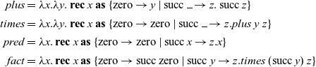 \begin{align*} \mathit{plus} &= \lambda x. \lambda y. \operatorname{\mathbf{rec}} x \operatorname{\mathbf{as}} \ \{ \operatorname{zero} \to y \mid \operatorname{succ} \rule{1ex}{0.5pt} \to z. \operatorname{succ} z \} \\ \mathit{times} &= \lambda x. \lambda y. \operatorname{\mathbf{rec}} x \operatorname{\mathbf{as}} \ \{ \operatorname{zero} \to \operatorname{zero} \mid \operatorname{succ} \rule{1ex}{0.5pt} \to z. \mathit{plus}~y~z \} \\ \mathit{pred} &= \lambda x. \operatorname{\mathbf{rec}} x \operatorname{\mathbf{as}} \ \{ \operatorname{zero} \to \operatorname{zero} \mid \operatorname{succ} x \to z.x \} \\ \mathit{fact} &= \lambda x. \operatorname{\mathbf{rec}} x \operatorname{\mathbf{as}} \ \{ \operatorname{zero} \to \operatorname{succ}\operatorname{zero} \mid \operatorname{succ} y \to z. \mathit{times}~(\operatorname{succ} y)~z \}\end{align*}
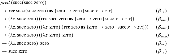
Executing $pred~(\operatorname{succ}(\operatorname{succ}\operatorname{zero}))$
in call-by-name proceeds like so:
$pred~(\operatorname{succ}(\operatorname{succ}\operatorname{zero}))$
in call-by-name proceeds like so:
 \begin{align*} & \mathit{pred}~(\operatorname{succ}(\operatorname{succ}\operatorname{zero})) \\ &\mapsto \operatorname{\mathbf{rec}} \operatorname{succ}(\operatorname{succ}\operatorname{zero}) \operatorname{\mathbf{as}} \ \{ \operatorname{zero} \to \operatorname{zero} \mid \operatorname{succ} x \to z.x \} &&(\beta_\to) \\ &\mapsto (\lambda z. \operatorname{succ}\operatorname{zero}) ~ (\operatorname{\mathbf{rec}} \operatorname{succ}\operatorname{zero} \operatorname{\mathbf{as}} \ \{ \operatorname{zero} \to \operatorname{zero} \mid \operatorname{succ} x \to z.x \}) &&(\beta_{\operatorname{succ}}) \\ &\mapsto \operatorname{succ}\operatorname{zero} &&(\beta_\to)\end{align*}
However, in call-by-value, the predecessor of both $\operatorname{succ} \operatorname{zero}$
and
$\operatorname{succ} \operatorname{zero}$
and $\operatorname{zero}$
is computed even though these intermediate results are not needed in the end:
$\operatorname{zero}$
is computed even though these intermediate results are not needed in the end:
 \begin{align*} & \mathit{pred}~(\operatorname{succ}(\operatorname{succ}\operatorname{zero})) \\ &\mapsto \operatorname{\mathbf{rec}} \operatorname{succ}(\operatorname{succ}\operatorname{zero}) \operatorname{\mathbf{as}} \ \{ \operatorname{zero} \to \operatorname{zero} \mid \operatorname{succ} x \to z.x \} &&(\beta_\to) \\ &\mapsto (\lambda z. \operatorname{succ}\operatorname{zero}) ~ (\operatorname{\mathbf{rec}} \operatorname{succ}\operatorname{zero} \operatorname{\mathbf{as}} \ \{ \operatorname{zero} \to \operatorname{zero} \mid \operatorname{succ} x \to z.x \}) &&(\beta_{\operatorname{succ}}) \\ &\mapsto (\lambda z. \operatorname{succ}\operatorname{zero}) ~ ((\lambda z.\operatorname{zero}) ~ (\operatorname{\mathbf{rec}} \operatorname{zero} \operatorname{\mathbf{as}} \ \{ \operatorname{zero} \to \operatorname{zero} \mid \operatorname{succ} x \to z.x \})) &&(\beta_{\operatorname{succ}}) \\ &\mapsto (\lambda z. \operatorname{succ}\operatorname{zero})~ ((\lambda z.\operatorname{zero}) ~ \operatorname{zero}) &&(\beta_{\operatorname{zero}}) \\ &\mapsto (\lambda z. \operatorname{succ}\operatorname{zero}) ~ \operatorname{zero} &&(\beta_\to) \\ &\mapsto \operatorname{succ}\operatorname{zero} &&(\beta_\to)\end{align*}
In general, $\mathit{pred}$
is a constant time (O(1)) function over the size of its argument when following the call-by-name semantics, which computes the predecessor of any natural number in a fixed number of steps. In contrast,
$\mathit{pred}$
is a constant time (O(1)) function over the size of its argument when following the call-by-name semantics, which computes the predecessor of any natural number in a fixed number of steps. In contrast, $\mathit{pred}$
is a linear time (O(n)) function when following the call-by-value semantics, where
$\mathit{pred}$
is a linear time (O(n)) function when following the call-by-value semantics, where $\mathit{pred}~(\operatorname{succ}^n\operatorname{zero})$
executes with a number of steps proportional to the size n of its argument because it requires at least n applications of the
$\mathit{pred}~(\operatorname{succ}^n\operatorname{zero})$
executes with a number of steps proportional to the size n of its argument because it requires at least n applications of the $\beta_{\operatorname{succ}}$
rule before an answer can be returned.
$\beta_{\operatorname{succ}}$
rule before an answer can be returned.
3 Recursion in an abstract machine
In order to explore the lower-level performance details of recursion, we can use an abstract machine for modeling an implementation of System T. Please suggest whether the spelling of the term ’redex’ in the sentence ’Unlike the reduction step’ is OK.Unlike the operational semantics given in Fig. 3, which requires a costly recursive search deep into an expression to find the next redex at every step, an abstract machine explicitly includes this search in the computation itself which can immediately resume from the same position as the previous reduction step. As such, every step of the machine can be applied by matching only on the top-level form of the machine state, which models the fact that a real implementations in a machine does not have to recursively search for the next reduction step to perform, but can identify and jump to the next step in a constant amount of time. Thus, in an abstract machine instead of working with terms one works with configurations of the form:
 $$\langle {M} |\!| {E} \rangle$$
where M is a term also called a producer and E is a continuation or evaluation context, also called a consumer. A state, also called a command, puts together a producer and a consumer, so that the output of M is given as the input to E. We first present distinct abstract machines for call-by-name and call-by-value, we then smooth out the differences in the uniform abstract machine.
3.1 Call-by-name abstract machine
The call-by-name abstract machine for System T is based on the Krivine machine (Krivine, 2007), which is defined in terms of these continuations (representing evaluation contexts, for example, $\operatorname{\mathbf{tp}}$
represents the empty, top-level context) and transition rules:
Footnote 1
$\operatorname{\mathbf{tp}}$
represents the empty, top-level context) and transition rules:
Footnote 1 $^{\kern-1pt,}$
Footnote 2
$^{\kern-1pt,}$
Footnote 2
 \begin{align*} E &::= \operatorname{\mathbf{tp}} \mid N \cdot E \mid \operatorname{\mathbf{rec}} \{ \operatorname{zero} \to M \mid \operatorname{succ} x \to z. N \} \operatorname{\mathbf{with}} E\end{align*}
Refocusing rules:
 \begin{align*} \langle {M~N} |\!| {E} \rangle &\mapsto \langle {M} |\!| {N \cdot E} \rangle \\ \langle {\operatorname{\mathbf{rec}} M \operatorname{\mathbf{as}} \{\dots\} } |\!| {E} \rangle &\mapsto \langle {M} |\!| {\operatorname{\mathbf{rec}} \{\dots\} \operatorname{\mathbf{with}} E} \rangle\end{align*}
Reduction rules:

The first two rules are refocusing rules that move the attention of the machine closer to the next reduction building a larger continuation: $N \cdot E$
corresponds to the context
$N \cdot E$
corresponds to the context $E[\square~N]$
, and the continuation
$E[\square~N]$
, and the continuation $\operatorname{\mathbf{rec}} \{\operatorname{zero} \to N \mid \operatorname{succ} x \to y.N'\} \operatorname{\mathbf{with}} E$
corresponds to the context
$\operatorname{\mathbf{rec}} \{\operatorname{zero} \to N \mid \operatorname{succ} x \to y.N'\} \operatorname{\mathbf{with}} E$
corresponds to the context $E[\operatorname{\mathbf{rec}} \square \operatorname{\mathbf{as}} \{\operatorname{zero} \to N \mid \operatorname{succ} x \to y.N'\} ]$
. The latter three rules are reduction rules which correspond to steps of the operational semantics in Fig. 3. While the distinction between refocusing and reduction rules is just a mere classification now, the difference will become an important tool for generalizing the abstract machine into a more uniform presentation later in Section 3.3.
$E[\operatorname{\mathbf{rec}} \square \operatorname{\mathbf{as}} \{\operatorname{zero} \to N \mid \operatorname{succ} x \to y.N'\} ]$
. The latter three rules are reduction rules which correspond to steps of the operational semantics in Fig. 3. While the distinction between refocusing and reduction rules is just a mere classification now, the difference will become an important tool for generalizing the abstract machine into a more uniform presentation later in Section 3.3.
3.2 Call-by-value abstract machine
A CEK-style (Felleisen & Friedman, 1986), call-by-value abstract machine for System T—which evaluates applications $M_1~M_2~\dots~M_n$
left-to-right to match the call-by-value semantics in Fig. 3—is given by these continuations E and transition rules:
$M_1~M_2~\dots~M_n$
left-to-right to match the call-by-value semantics in Fig. 3—is given by these continuations E and transition rules:
 \begin{align*} E &::= \operatorname{\mathbf{tp}} \mid n \cdot E \mid V \circ E \mid \operatorname{succ} \circ E \mid \operatorname{\mathbf{rec}} \{\operatorname{zero} \to M \mid \operatorname{succ} x \to y. N\} \operatorname{\mathbf{with}} E\end{align*}
Refocusing rules:
 \begin{align*} \langle {M~N} |\!| {E} \rangle &\mapsto \langle {M} |\!| {N \cdot E} \rangle \\ \langle {V} |\!| {R \cdot E} \rangle &\mapsto \langle {R} |\!| {V \circ E} \rangle \\ \langle {V} |\!| {V' \circ E} \rangle &\mapsto \langle {V'} |\!| {V \cdot E} \rangle \\ \langle {\operatorname{\mathbf{rec}} M \operatorname{\mathbf{as}} \{\dots\}} |\!| {E} \rangle &\mapsto \langle {M} |\!| {\operatorname{\mathbf{rec}} \{\dots\} \operatorname{\mathbf{with}} E} \rangle \\ \langle {\operatorname{succ} R} |\!| {E} \rangle &\mapsto \langle {R} |\!| {\operatorname{succ} \circ E} \rangle \\ \langle {V} |\!| {\operatorname{succ} \circ E} \rangle &\mapsto \langle {\operatorname{succ} V} |\!| {E} \rangle\end{align*}
Reduction rules:

where R stands for a non-value term. Since the call-by-value operational semantics has more forms of evaluation contexts, this machine has additional refocusing rules for accumulating more forms of continuations including applications of functions ( $V \circ E$
corresponding to
$V \circ E$
corresponding to $E[V~\square]$
) and the successor constructor (
$E[V~\square]$
) and the successor constructor ( $\operatorname{succ} \circ E$
corresponding to
$\operatorname{succ} \circ E$
corresponding to $E[\operatorname{succ}~\square]$
). Also note that the final reduction rule for the
$E[\operatorname{succ}~\square]$
). Also note that the final reduction rule for the $\operatorname{succ}$
case of recursion is different, accounting for the fact that recursion in call-by-value follows a different order than in call-by-name. Indeed, the recursor must explicitly accumulate and build upon a continuation, “adding to” the place it returns to with every recursive call. But otherwise, the reduction rules are the same.
Footnote 3
$\operatorname{succ}$
case of recursion is different, accounting for the fact that recursion in call-by-value follows a different order than in call-by-name. Indeed, the recursor must explicitly accumulate and build upon a continuation, “adding to” the place it returns to with every recursive call. But otherwise, the reduction rules are the same.
Footnote 3
3.3 Uniform abstract machine
We now unite both evaluation strategies with a common abstract machine, shown in Fig. 4. As before, machine configurations are of the form
 $$\langle {v} |\!| {e} \rangle$$
which put together a term v and a continuation e (often referred to as a coterm). However, both terms and continuations are more general than before. Our uniform abstract machine is based on the sequent calculus, a symmetric language reflecting many dualities of classical logic (Curien & Herbelin, 2000; Wadler, Reference Wadler2003). An advantage of this sequent-based system is that the explicit symmetry inherent in its syntax gives us a language to express and understand the implicit symmetries that are hiding in computations and types. This utility of a symmetric language is one of the key insights of our approach, which will let us syntactically derive a notion of corecursion which is dual to recursion.
Uniform, recursive abstract machine for System T.

Unlike the previous machines, continuations go beyond evaluation contexts and include ${\tilde{\mu}}{x}. \langle {v} |\!| {e} \rangle$
, which is a continuation that binds its input value to x and then steps to the machine state
${\tilde{\mu}}{x}. \langle {v} |\!| {e} \rangle$
, which is a continuation that binds its input value to x and then steps to the machine state $\langle {v} |\!| {e} \rangle$
. This new form allows us to express the additional call-by-value evaluation contexts:
$\langle {v} |\!| {e} \rangle$
. This new form allows us to express the additional call-by-value evaluation contexts: $V \circ E$
becomes
$V \circ E$
becomes ${\tilde{\mu}}{x}. \langle {V} |\!| {x \cdot E} \rangle$
, and
${\tilde{\mu}}{x}. \langle {V} |\!| {x \cdot E} \rangle$
, and $\operatorname{succ} \circ E$
is
$\operatorname{succ} \circ E$
is ${\tilde{\mu}}{x}. \langle {\operatorname{succ} x} |\!| {E} \rangle$
. Evaluation contexts are also more restrictive than before; only values can be pushed on the calling stack. We represent the application continuation
${\tilde{\mu}}{x}. \langle {\operatorname{succ} x} |\!| {E} \rangle$
. Evaluation contexts are also more restrictive than before; only values can be pushed on the calling stack. We represent the application continuation $M \cdot E$
with a non-value argument M by naming its partner—the generic value V—with y:
$M \cdot E$
with a non-value argument M by naming its partner—the generic value V—with y: $ {\tilde{\mu}}{y}. \langle {M} |\!| {{\tilde{\mu}}{x}. \langle {y} |\!| {x \cdot E} \rangle} \rangle$
.
Footnote 4
$ {\tilde{\mu}}{y}. \langle {M} |\!| {{\tilde{\mu}}{x}. \langle {y} |\!| {x \cdot E} \rangle} \rangle$
.
Footnote 4
The refocusing rules can be subsumed all together by extending terms with a dual form of ${\tilde{\mu}}$
-binding. The
${\tilde{\mu}}$
-binding. The $\mu$
-abstraction expression
$\mu$
-abstraction expression $\mu{\alpha}. \langle {v} |\!| {e} \rangle$
binds its continuation to
$\mu{\alpha}. \langle {v} |\!| {e} \rangle$
binds its continuation to $\alpha$
and then steps to the machine state
$\alpha$
and then steps to the machine state $\langle {v} |\!| {e} \rangle$
. With
$\langle {v} |\!| {e} \rangle$
. With $\mu$
-bindings, all the refocusing rules for call-by-name and call-by-value can be encoded in terms of
$\mu$
-bindings, all the refocusing rules for call-by-name and call-by-value can be encoded in terms of $\mu$
and
$\mu$
and ${\tilde{\mu}}$
.
Footnote 5
It is also not necessary to do these steps at run-time, but can all be done before execution through a compilation step. The target language of this compilation step becomes the syntax of the uniform abstract machine, as shown in Fig. 4. This language does not include anymore applications
${\tilde{\mu}}$
.
Footnote 5
It is also not necessary to do these steps at run-time, but can all be done before execution through a compilation step. The target language of this compilation step becomes the syntax of the uniform abstract machine, as shown in Fig. 4. This language does not include anymore applications $M~N$
and the recursive term
$M~N$
and the recursive term $\operatorname{\mathbf{rec}} M \operatorname{\mathbf{as}} \{\dots\}$
. Also, unlike System T, the syntax of terms and coterms depends on the definition of values and covalues;
$\operatorname{\mathbf{rec}} M \operatorname{\mathbf{as}} \{\dots\}$
. Also, unlike System T, the syntax of terms and coterms depends on the definition of values and covalues; $\operatorname{succ} V$
,
$\operatorname{succ} V$
, $\operatorname{\mathbf{rec}} \{\dots\} \operatorname{\mathbf{with}} E$
, and call stacks
$\operatorname{\mathbf{rec}} \{\dots\} \operatorname{\mathbf{with}} E$
, and call stacks $V \cdot E$
are valid in both call-by-name and call-by-value, just with different definitions of V and E. Yet, all System T terms can still be translated to the smaller language of the machine, as shown in Fig. 5. General terms also include the
$V \cdot E$
are valid in both call-by-name and call-by-value, just with different definitions of V and E. Yet, all System T terms can still be translated to the smaller language of the machine, as shown in Fig. 5. General terms also include the $\mu$
- and
$\mu$
- and ${\tilde{\mu}}$
-binders described above:
${\tilde{\mu}}$
-binders described above: $\mu{\alpha}. c$
is not a value in call-by-value, and
$\mu{\alpha}. c$
is not a value in call-by-value, and ${\tilde{\mu}}{x}. c$
is not a covalue in call-by-name. So for example,
${\tilde{\mu}}{x}. c$
is not a covalue in call-by-name. So for example, $\operatorname{succ} (\mu{\alpha}. c)$
is not a legal term in call-by-value, but can be translated instead to
$\operatorname{succ} (\mu{\alpha}. c)$
is not a legal term in call-by-value, but can be translated instead to $\mu{\beta}. \langle {\mu{\alpha}. c} |\!| {{\tilde{\mu}}{x}. \langle {\operatorname{succ} x} |\!| {\beta} \rangle} \rangle$
following Fig. 5. Similarly
$\mu{\beta}. \langle {\mu{\alpha}. c} |\!| {{\tilde{\mu}}{x}. \langle {\operatorname{succ} x} |\!| {\beta} \rangle} \rangle$
following Fig. 5. Similarly $x \cdot {\tilde{\mu}}{y}. c$
is not a legal call stack in call-by-name, but it can be rewritten to
$x \cdot {\tilde{\mu}}{y}. c$
is not a legal call stack in call-by-name, but it can be rewritten to ${\tilde{\mu}}{z}. \langle {\mu{\alpha}.\langle {z} |\!| {x \cdot \alpha} \rangle} |\!| {{\tilde{\mu}}{y}. c} \rangle$
.
${\tilde{\mu}}{z}. \langle {\mu{\alpha}.\langle {z} |\!| {x \cdot \alpha} \rangle} |\!| {{\tilde{\mu}}{y}. c} \rangle$
.
The translation from System T to the uniform abstract machine.

As with System T, the notions of values and covalues drive the reduction rules in Fig. 4. In particular, the $\mu$
and
$\mu$
and ${\tilde{\mu}}$
rules will only substitute a value for a variable or a covalue for a covariable, respectively. Likewise, the
${\tilde{\mu}}$
rules will only substitute a value for a variable or a covalue for a covariable, respectively. Likewise, the $\beta_\to$
rule implements function calls, but taking the next argument value off of a call stack and plugging it into the function. The only remaining rules are
$\beta_\to$
rule implements function calls, but taking the next argument value off of a call stack and plugging it into the function. The only remaining rules are $\beta_{\operatorname{zero}}$
and
$\beta_{\operatorname{zero}}$
and $\beta_{\operatorname{succ}}$
for reducing a recursor when given a number constructed by
$\beta_{\operatorname{succ}}$
for reducing a recursor when given a number constructed by $\operatorname{zero}$
or
$\operatorname{zero}$
or $\operatorname{succ}$
. While the
$\operatorname{succ}$
. While the $\beta_{\operatorname{zero}}$
is exactly the same as it was previously in both specialized machine, notice how
$\beta_{\operatorname{zero}}$
is exactly the same as it was previously in both specialized machine, notice how $\beta_{\operatorname{succ}}$
is different. Rather than committing to one evaluation order or the other,
$\beta_{\operatorname{succ}}$
is different. Rather than committing to one evaluation order or the other, $\beta_{\operatorname{succ}}$
is neutral: the recursive predecessor (expressed as the term
$\beta_{\operatorname{succ}}$
is neutral: the recursive predecessor (expressed as the term $\mu{\alpha}.\langle {V} |\!| {\operatorname{\mathbf{rec}}\{\dots\}\operatorname{\mathbf{with}}\alpha} \rangle$
on the right-hand side) is neither given precedence (at the top of the command) nor delayed (by substituting it for y). Instead, this recursive predecessor is bound to y with a
$\mu{\alpha}.\langle {V} |\!| {\operatorname{\mathbf{rec}}\{\dots\}\operatorname{\mathbf{with}}\alpha} \rangle$
on the right-hand side) is neither given precedence (at the top of the command) nor delayed (by substituting it for y). Instead, this recursive predecessor is bound to y with a ${\tilde{\mu}}$
-abstraction. This way, the correct evaluation order can be decided in the next step by either an application of
${\tilde{\mu}}$
-abstraction. This way, the correct evaluation order can be decided in the next step by either an application of $\mu$
or
$\mu$
or ${\tilde{\mu}}$
reduction.
${\tilde{\mu}}$
reduction.
Notice one more advantage of translating System T at “compile-time” into a smaller language in the abstract machine. In the same way that the $\lambda$
-calculus supports both a deterministic operational semantics along with a rewriting system that allows for optimizations that apply reductions to any sub-expression, so too does the syntax of this uniform abstract machine allow for optimizations that reduce sub-expressions in advance of the usual execution order. For example, consider the term
$\lambda$
-calculus supports both a deterministic operational semantics along with a rewriting system that allows for optimizations that apply reductions to any sub-expression, so too does the syntax of this uniform abstract machine allow for optimizations that reduce sub-expressions in advance of the usual execution order. For example, consider the term $\operatorname{\mathbf{let}} f = (\lambda{x}. (\lambda{y}. y)~x) \operatorname{\mathbf{in}} M$
.
Footnote 6
Its next step is to substitute the abstraction
$\operatorname{\mathbf{let}} f = (\lambda{x}. (\lambda{y}. y)~x) \operatorname{\mathbf{in}} M$
.
Footnote 6
Its next step is to substitute the abstraction $(\lambda{x}. (\lambda{y}. y)~x)$
for f in M, and every time M calls
$(\lambda{x}. (\lambda{y}. y)~x)$
for f in M, and every time M calls $(f~V)$
we must repeat the steps
$(f~V)$
we must repeat the steps
 \begin{align*} (\lambda{x}. (\lambda{y}. y)~x)~V \mapsto (\lambda{y}. y)~V \mapsto V\end{align*}
again. But applying a
\begin{align*} (\lambda{x}. (\lambda{y}. y)~x)~V \mapsto (\lambda{y}. y)~V \mapsto V\end{align*}
again. But applying a $\beta$
reduction under the
$\beta$
reduction under the $\lambda$
bound to f, we can instead optimize this expression to
$\lambda$
bound to f, we can instead optimize this expression to $\operatorname{\mathbf{let}} f = (\lambda{x}. x) \operatorname{\mathbf{in}} M$
. With this optimization, when M calls
$\operatorname{\mathbf{let}} f = (\lambda{x}. x) \operatorname{\mathbf{in}} M$
. With this optimization, when M calls $(f~V)$
it reduces as
$(f~V)$
it reduces as $(\lambda{x}. x)~V \mapsto V$
in one step. This same approach applies to the uniform abstract machine, too, because all elimination forms like
$(\lambda{x}. x)~V \mapsto V$
in one step. This same approach applies to the uniform abstract machine, too, because all elimination forms like $\square~N$
and
$\square~N$
and $\operatorname{\mathbf{rec}} \square \operatorname{\mathbf{as}} \{\dots\}$
have been compiled to continuations of the form
$\operatorname{\mathbf{rec}} \square \operatorname{\mathbf{as}} \{\dots\}$
have been compiled to continuations of the form $N \cdot \alpha$
and
$N \cdot \alpha$
and $\operatorname{\mathbf{rec}}\{\dots\}\operatorname{\mathbf{with}}\alpha$
that we can use to apply machine reductions. For example, the translation of
$\operatorname{\mathbf{rec}}\{\dots\}\operatorname{\mathbf{with}}\alpha$
that we can use to apply machine reductions. For example, the translation of $\operatorname{\mathbf{let}} f = (\lambda{x}. (\lambda{y}. y)~x) \operatorname{\mathbf{in}} M$
is quite large, but we can optimize away several
$\operatorname{\mathbf{let}} f = (\lambda{x}. (\lambda{y}. y)~x) \operatorname{\mathbf{in}} M$
is quite large, but we can optimize away several $\mu$
and
$\mu$
and ${\tilde{\mu}}$
reductions—which are responsible for the administrative duty of directing information and control flow—in advance inside sub-expressions to simplify the translation to:
Footnote 7
${\tilde{\mu}}$
reductions—which are responsible for the administrative duty of directing information and control flow—in advance inside sub-expressions to simplify the translation to:
Footnote 7
where $\mathrel{\to\!\!\!\!\to}$
denotes zero or more reduction steps
$\mathrel{\to\!\!\!\!\to}$
denotes zero or more reduction steps $\mapsto$
applied inside any context. From there, we can further optimize the program by simplifying the application of
$\mapsto$
applied inside any context. From there, we can further optimize the program by simplifying the application of $\lambda{y}. y$
in advance, by applying the
$\lambda{y}. y$
in advance, by applying the $\beta_\to$
rule inside the
$\beta_\to$
rule inside the $\mu$
s binding
$\mu$
s binding $\alpha$
and
$\alpha$
and $\beta$
and the
$\beta$
and the $\lambda$
binding x like so:
$\lambda$
binding x like so:
This way, we are able to still optimize the program even after compilation to the abstract machine language, the same as if we were optimizing the original $\lambda$
-calculus source code.
$\lambda$
-calculus source code.
Intermezzo 3.1 We can now summarize how some basic concepts of recursion are directly modeled in our syntactic framework:
– With inductive data types, values are constructed and the consumer is a recursive process that uses the data. Natural numbers are terms or producers, and their use is a process which is triggered when the term becomes a value.
– Construction of data is finite and its consumption is (potentially) infinite, in the sense that there must be no limit to the size of the data that a consumer can process. We can only build values from a finite number of constructor applications. However, the consumer does not know how big of an input it will be given, so it has to be ready to handle data structures of any size. In the end, termination is preserved because only finite values are consumed.
– Recursion uses the data, rather than producing it. $\operatorname{\mathbf{rec}}$
is a coterm, not a term.
$\operatorname{\mathbf{rec}}$
is a coterm, not a term.– Recursion starts big and potentially reduces down to a base case. As shown in the reduction rules, the recursor breaks down the data structure and might end when the base case is reached.
– The values of a data structures are all independent from each other but the results of the recursion potentially depend on each other. In the reduction rule for the successor case, the result at a number n might depend on the result at
$n-1$
.


3.4 Examples of recursion
Restricting the $\mu$
and
$\mu$
and ${\tilde{\mu}}$
rules to only binding (co)values effectively implements the chosen evaluation strategy. For example, consider the application
${\tilde{\mu}}$
rules to only binding (co)values effectively implements the chosen evaluation strategy. For example, consider the application $(\lambda z. \operatorname{succ}\operatorname{zero})~((\lambda x. x)~\operatorname{zero})$
. Call-by-name evaluation will reduce the outer application first and return
$(\lambda z. \operatorname{succ}\operatorname{zero})~((\lambda x. x)~\operatorname{zero})$
. Call-by-name evaluation will reduce the outer application first and return $\operatorname{succ}\operatorname{zero}$
right away, whereas call-by-value evaluation will first reduce the inner application
$\operatorname{succ}\operatorname{zero}$
right away, whereas call-by-value evaluation will first reduce the inner application $((\lambda x.x)~\operatorname{zero})$
. How is this different order of evaluation made explicit in the abstract machine, which uses the same set of rules in both cases? First, consider the translation of
$((\lambda x.x)~\operatorname{zero})$
. How is this different order of evaluation made explicit in the abstract machine, which uses the same set of rules in both cases? First, consider the translation of $[\![ (\lambda z. x)~((\lambda x. x)~y) ]\!]$
:
$[\![ (\lambda z. x)~((\lambda x. x)~y) ]\!]$
:
This is quite a large term for such a simple source expression. To make the example clearer, let us first simplify the administrative-style ${\tilde{\mu}}$
-bindings out of the way (using applications of
${\tilde{\mu}}$
-bindings out of the way (using applications of ${\tilde{\mu}}$
rules for to substitute
${\tilde{\mu}}$
rules for to substitute $\lambda$
-abstractions and variables in a way that is valid for both call-by-name and call-by-value) to get the shorter term:
$\lambda$
-abstractions and variables in a way that is valid for both call-by-name and call-by-value) to get the shorter term:
 \begin{align*} [\![ (\lambda z. x)~((\lambda x. x)~y) ]\!] &\mathrel{\to\!\!\!\!\to}_{{\tilde{\mu}}} \mu{\alpha}. \langle {\mu{\beta}.\langle {\lambda x. x} |\!| {y \cdot \beta} \rangle} |\!| {} {{\tilde{\mu}}{z}. \langle {\lambda z. x} |\!| {z \cdot \alpha} \rangle \rangle}\end{align*}
To execute it, we need to put it in interaction with an actual context. In our case, we can simply use a covariable $\alpha$
. Call-by-name execution then proceeds from the simplified as:
$\alpha$
. Call-by-name execution then proceeds from the simplified as:
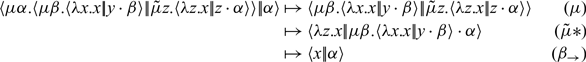
And call-by-value execution of the simplified proceeds as:
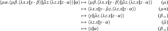
The first two steps are the same for either evaluation strategy. Where the two begin to diverge is in the third step (marked by a $*$
), which is an interaction between a
$*$
), which is an interaction between a $\mu$
- and a
$\mu$
- and a ${\tilde{\mu}}$
-binder. In call-by-name, the
${\tilde{\mu}}$
-binder. In call-by-name, the ${\tilde{\mu}}$
rule takes precedence (because a
${\tilde{\mu}}$
rule takes precedence (because a ${\tilde{\mu}}$
-coterm is not a covalue), leading to the next step which throws away the first argument, unevaluated. In call-by-value, the
${\tilde{\mu}}$
-coterm is not a covalue), leading to the next step which throws away the first argument, unevaluated. In call-by-value, the $\mu$
rule takes precedence (because a
$\mu$
rule takes precedence (because a $\mu$
-term is not a value), leading to the next step which evaluates the first argument, producing y to bind to z that eventually gets thrown away.
$\mu$
-term is not a value), leading to the next step which evaluates the first argument, producing y to bind to z that eventually gets thrown away.
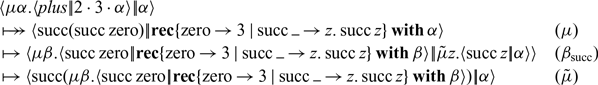
Consider the System T definition of $\mathit{plus}$
from Example 2.1, which is expressed by the machine term
$\mathit{plus}$
from Example 2.1, which is expressed by the machine term
The application $\mathit{plus}~2~3$
is then expressed as
$\mathit{plus}~2~3$
is then expressed as $ \mu{\alpha}. \langle {\mathit{plus}} |\!| { } \rangle {2 \cdot 3 \cdot \alpha}$
, which is obtained by reducing some
$ \mu{\alpha}. \langle {\mathit{plus}} |\!| { } \rangle {2 \cdot 3 \cdot \alpha}$
, which is obtained by reducing some $\mu$
- and
$\mu$
- and ${\tilde{\mu}}$
-bindings in advance. Putting this term in the context
${\tilde{\mu}}$
-bindings in advance. Putting this term in the context $\alpha$
, in call-by-value it executes (eliding the branches of the
$\alpha$
, in call-by-value it executes (eliding the branches of the $\operatorname{\mathbf{rec}}$
continuation, which are the same in every following step) like so:
$\operatorname{\mathbf{rec}}$
continuation, which are the same in every following step) like so:

Notice how this execution shows how, during the recursive traversal of the data structure, the return continuation of the recursor is updated (in blue) to keep track of the growing context of pending operations, which must be fully processed before the final value of 5 ( $\operatorname{succ}(\operatorname{succ} 3)$
) can be returned to the original caller (
$\operatorname{succ}(\operatorname{succ} 3)$
) can be returned to the original caller ( $\alpha$
). This update is implicit in the
$\alpha$
). This update is implicit in the $\lambda$
-calculus-based System T, but becomes explicit in the abstract machine. In contrast, call-by-name only computes numbers as far as they are needed, otherwise stopping at the outermost constructor. The call-by-name execution of the above command proceeds as follows, after fast-forwarding to the first application of
$\lambda$
-calculus-based System T, but becomes explicit in the abstract machine. In contrast, call-by-name only computes numbers as far as they are needed, otherwise stopping at the outermost constructor. The call-by-name execution of the above command proceeds as follows, after fast-forwarding to the first application of $\beta_{\operatorname{succ}}$
:
$\beta_{\operatorname{succ}}$
:
Unless $\alpha$
demands to know something about the predecessor of this number, the term
$\alpha$
demands to know something about the predecessor of this number, the term $\mu{\beta}.\langle {\operatorname{succ}\operatorname{zero}} |\!| {\operatorname{\mathbf{rec}}\{\dots\}\operatorname{\mathbf{with}}\beta} \rangle$
will not be computed.
$\mu{\beta}.\langle {\operatorname{succ}\operatorname{zero}} |\!| {\operatorname{\mathbf{rec}}\{\dots\}\operatorname{\mathbf{with}}\beta} \rangle$
will not be computed.
Now consider $\mathit{pred}~(\operatorname{succ}(\operatorname{succ}\operatorname{zero}))$
, which can be expressed in the machine as:
$\mathit{pred}~(\operatorname{succ}(\operatorname{succ}\operatorname{zero}))$
, which can be expressed in the machine as:
 \begin{align*} & \mu{\alpha}. \langle {\mathit{pred}} |\!| {} \rangle {\operatorname{succ}(\operatorname{succ}\operatorname{zero}) \cdot \alpha} \\ \mathit{pred} &= \lambda x. \mu{\beta}.\langle {x} |\!| {\operatorname{\mathbf{rec}}\{\operatorname{zero}\to\operatorname{zero}\mid\operatorname{succ} x\to z.x\}\operatorname{\mathbf{with}}\beta} \rangle\end{align*}
In call-by-name, it executes with respect to $\alpha$
like so:
$\alpha$
like so:

Notice how, after the first application of $\beta_{\operatorname{succ}}$
, the computation finishes in just one
$\beta_{\operatorname{succ}}$
, the computation finishes in just one ${\tilde{\mu}}$
step, even though we began recursing on the number 2. In call-by-value instead, we have to continue with the recursion even though its result is not needed. Fast-forwarding to the first application of the
${\tilde{\mu}}$
step, even though we began recursing on the number 2. In call-by-value instead, we have to continue with the recursion even though its result is not needed. Fast-forwarding to the first application of the $\beta_{\operatorname{succ}}$
rule, we have:
$\beta_{\operatorname{succ}}$
rule, we have:

3.5 Recursion versus iteration: Expressiveness and efficiency
Recall how the recursor performs two jobs at the same time: finding the predecessor of a natural number as well as calculating the recursive result given for the predecessor. These two functionalities can be captured separately by continuations that perform shallow case analysis and iteration, respectively. Rather than including them as primitives, both can be expressed as syntactic sugar in the form of macro-expansions in the language of the abstract machine like so:
 \begin{align*}\begin{aligned} & \operatorname{\mathbf{case}} \begin{alignedat}[t]{2} \{& \operatorname{zero} &&\to v \\ \mid& \operatorname{succ} x &&\to w \} \end{alignedat} \\ &\operatorname{\mathbf{with}} E\end{aligned}&:=\!\!\begin{aligned} &\operatorname{\mathbf{rec}} \begin{alignedat}[t]{2} \{& \operatorname{zero} &&\to v \\ \mid& \operatorname{succ} x &&\to \rule{1ex}{0.5pt}\,. w \} \end{alignedat} \\ &\operatorname{\mathbf{with}} E\end{aligned}&~~\begin{aligned} & \operatorname{\mathbf{iter}} \begin{alignedat}[t]{2} \{& \operatorname{zero} &&\to v \\ \mid& \operatorname{succ} &&\to x.w \} \end{alignedat} \\ &\operatorname{\mathbf{with}} E\end{aligned}&:=\!\!\begin{aligned} &\operatorname{\mathbf{rec}} \begin{alignedat}[t]{2} \{& \operatorname{zero} &&\to v \\ \mid& \operatorname{succ} \rule{1ex}{0.5pt} &&\to x.w \} \end{alignedat} \\ &\operatorname{\mathbf{with}} E\end{aligned}\end{align*}
The only cost of this encoding of $\operatorname{\mathbf{case}}$
and
$\operatorname{\mathbf{case}}$
and $\operatorname{\mathbf{iter}}$
is an unused variable binding, which is easily optimized away. In practice, this encoding of iteration will perform exactly the same as if we had taken
$\operatorname{\mathbf{iter}}$
is an unused variable binding, which is easily optimized away. In practice, this encoding of iteration will perform exactly the same as if we had taken $\operatorname{\mathbf{iter}}$
ation as a primitive.
$\operatorname{\mathbf{iter}}$
ation as a primitive.
While it is less obvious, going the other way is still possible. It is well known that primitive recursion can be encoded as a macro-expansion of iteration using pairs. The usual macro-expansion in System T is:
 \begin{align*} \begin{aligned} & \operatorname{\mathbf{rec}} M \operatorname{\mathbf{as}} \\ &\quad \begin{alignedat}{2} &\{~ \operatorname{zero} &&\to N \\ &\mid \operatorname{succ} x &&\to y. N' \} \end{alignedat} \end{aligned} &:= \begin{aligned} &\operatorname{snd}~ ( \operatorname{\mathbf{iter}} M \operatorname{\mathbf{as}} \\ &\qquad\quad \begin{alignedat}{2} &\{~ \operatorname{zero} &&\to (\operatorname{zero}, N) \\ &\mid \operatorname{succ} &&\to (x,y).\, (\operatorname{succ} x, N') \} ) \end{alignedat} \end{aligned}\end{align*}
The trick to this encoding is to use $\operatorname{\mathbf{iter}}$
to compute both a reconstruction of the number being iterated upon (the first component of the iterative result) alongside the desired result (the second component). Doing both at once gives access to the predecessor in the
$\operatorname{\mathbf{iter}}$
to compute both a reconstruction of the number being iterated upon (the first component of the iterative result) alongside the desired result (the second component). Doing both at once gives access to the predecessor in the $\operatorname{succ}$
case, which can be extracted from the first component of the previous result (given by the variable x in the pattern match (x,y)).
$\operatorname{succ}$
case, which can be extracted from the first component of the previous result (given by the variable x in the pattern match (x,y)).
To express this encoding in the abstract machine, we need to extend it with pairs, which look like (Wadler, Reference Wadler2003):
 \begin{align*} \langle {(v, w)} |\!| {\operatorname{fst} E} \rangle &\mapsto \langle {v} |\!| {E} \rangle & \langle {(v, w)} |\!| {\operatorname{snd} E} \rangle &\mapsto \langle {w} |\!| {E} \rangle & (\beta_\times)\end{align*}
In the syntax of the abstract machine, the analogous encoding of a $\operatorname{\mathbf{rec}}$
continuation as a macro-expansion looks like this:
$\operatorname{\mathbf{rec}}$
continuation as a macro-expansion looks like this:
 \begin{align*}\begin{aligned} &\operatorname{\mathbf{rec}} \begin{alignedat}[t]{2} \{& \operatorname{zero} &&\to v \\ \mid& \operatorname{succ} x &&\to y.w \} \end{alignedat} \\ &\operatorname{\mathbf{with}} E\end{aligned}&:=\begin{aligned} &\operatorname{\mathbf{iter}} \begin{alignedat}[t]{2} \{& \operatorname{zero} &&\to (\operatorname{zero}, v) \\ \mid& \operatorname{succ} &&\to (x,y). (\operatorname{succ} x, w) \} \end{alignedat} \\ &\operatorname{\mathbf{with}}{} \operatorname{snd} E\end{aligned}\end{align*}
Since the inductive case w might refer to both the predecessor x and the recursive result for the predecessor (named y), the two parts must be extracted from the pair returned from iteration. Here we express this extraction in the form of pattern matching, which is shorthand for:
 \begin{equation*} (x,y). (v_1,v_2) := z. \mu{\alpha}. \langle {z} |\!| {\operatorname{fst}({\tilde{\mu}}{x}. \langle {z} |\!| {\operatorname{snd}({\tilde{\mu}}{y}. \langle {(v_1,v_2)} |\!| {\alpha} \rangle)} \rangle)} \rangle\end{equation*}
Note that the recursor continuation is tasked with passing its final result to E once it has finished. In order to give this same result to E, the encoding has to extract the second component of the final pair before passing it to E, which is exactly what $\operatorname{snd} E$
expresses.
$\operatorname{snd} E$
expresses.
Unfortunately, this encoding of recursion is not always as efficient as the original. If the recursive parameter y is never used (such as in the $\mathit{pred}$
function), then
$\mathit{pred}$
function), then $\operatorname{\mathbf{rec}}$
can provide an answer without computing the recursive result. However, when encoding
$\operatorname{\mathbf{rec}}$
can provide an answer without computing the recursive result. However, when encoding $\operatorname{\mathbf{rec}}$
with
$\operatorname{\mathbf{rec}}$
with $\operatorname{\mathbf{iter}}$
, the result of the recursive value must always be computed before an answer is seen, regardless of whether or not y is needed. As such, redefining
$\operatorname{\mathbf{iter}}$
, the result of the recursive value must always be computed before an answer is seen, regardless of whether or not y is needed. As such, redefining $\mathit{pred}$
using
$\mathit{pred}$
using $\operatorname{\mathbf{iter}}$
in this way changes it from a constant time (O(1)) to a linear time (O(n)) function. Notice that this difference in cost is only apparent in call-by-name, which can be asymptotically more efficient when the recursive y is not needed to compute N’, as in
$\operatorname{\mathbf{iter}}$
in this way changes it from a constant time (O(1)) to a linear time (O(n)) function. Notice that this difference in cost is only apparent in call-by-name, which can be asymptotically more efficient when the recursive y is not needed to compute N’, as in $\mathit{pred}$
. In call-by-value, the recursor must descend to the base case anyway before the incremental recursive steps are propagated backward. That is to say, the call-by-value
$\mathit{pred}$
. In call-by-value, the recursor must descend to the base case anyway before the incremental recursive steps are propagated backward. That is to say, the call-by-value $\operatorname{\mathbf{rec}}$
has the same asymptotic complexity as its encoding via
$\operatorname{\mathbf{rec}}$
has the same asymptotic complexity as its encoding via $\operatorname{\mathbf{iter}}$
.
$\operatorname{\mathbf{iter}}$
.
3.6 Types and correctness
We can also give a type system directly for the abstract machine, as shown in Fig. 6. This system has judgments for assigning types to terms as usual: $\Gamma \vdash v : A$
says v produces an output of type A. In addition, there are also judgments for assigning types to coterms (
$\Gamma \vdash v : A$
says v produces an output of type A. In addition, there are also judgments for assigning types to coterms ( $\Gamma \vdash e \div A$
says e consumes an input of type A) and commands (
$\Gamma \vdash e \div A$
says e consumes an input of type A) and commands ( $\Gamma \vdash c \ $
says c is safe to compute, and does not produce or consume anything).
$\Gamma \vdash c \ $
says c is safe to compute, and does not produce or consume anything).
Type system for the uniform, recursive abstract machine.

This type system ensures that the machine itself is type safe: well-typed, executable commands don’t get stuck while in the process of computing a final state. For our purposes, we will consider “programs” to be commands c with just one free covariable (say $\alpha$
), representing the initial, top-level continuation expecting a natural number as the final answer. Thus, well-typed executable commands will satisfy
$\alpha$
), representing the initial, top-level continuation expecting a natural number as the final answer. Thus, well-typed executable commands will satisfy $\alpha\div\operatorname{Nat} \vdash c \ $
. The only final states of these programs have the form
$\alpha\div\operatorname{Nat} \vdash c \ $
. The only final states of these programs have the form $\langle {\operatorname{zero}} |\!| {\alpha} \rangle$
, which sends 0 to the final continuation
$\langle {\operatorname{zero}} |\!| {\alpha} \rangle$
, which sends 0 to the final continuation $\alpha$
, or
$\alpha$
, or
![]() , which sends the successor of some V to
, which sends the successor of some V to $\alpha$
. But the type system ensures more than just type safety: all well-typed programs will eventually terminate. That’s because
$\alpha$
. But the type system ensures more than just type safety: all well-typed programs will eventually terminate. That’s because $\operatorname{\mathbf{rec}}$
-expressions, which are the only form of recursion in the language, always decrement their input by 1 on each recursive step. So together, every well-typed executable command will eventually (termination) reach a valid final state (type safety).
$\operatorname{\mathbf{rec}}$
-expressions, which are the only form of recursion in the language, always decrement their input by 1 on each recursive step. So together, every well-typed executable command will eventually (termination) reach a valid final state (type safety).
Theorem 3.2 (Type safety & Termination of Programs). For any command c of the recursive abstract machine, if $\alpha\div\operatorname{Nat} \vdash c \ $
then
$\alpha\div\operatorname{Nat} \vdash c \ $
then $c \mathrel{\mapsto\!\!\!\!\to} \langle {\operatorname{zero}} |\!| {\alpha} \rangle$
or
$c \mathrel{\mapsto\!\!\!\!\to} \langle {\operatorname{zero}} |\!| {\alpha} \rangle$
or $c \mathrel{\mapsto\!\!\!\!\to} \langle {\operatorname{succ} V} |\!| {\alpha} \rangle$
for some V.
$c \mathrel{\mapsto\!\!\!\!\to} \langle {\operatorname{succ} V} |\!| {\alpha} \rangle$
for some V.
The truth of this theorem follows directly from the latter development in Section 6, since it is a special case of Theorem 6.14.
Intermezzo 3.3 Since our abstract machine is based on the logic of Gentzen’s sequent (Gentzen, 1935), the type system in Fig. 6 too can be viewed as a term assignment for a particular sequent calculus. In particular, the statement $v : A$
corresponds to a proof that A is true. Dually
$v : A$
corresponds to a proof that A is true. Dually $e \div A$
corresponds to a proof that A is false, and hence the notation, which can be understood as a built-in negation
$e \div A$
corresponds to a proof that A is false, and hence the notation, which can be understood as a built-in negation $-$
in
$-$
in $e : -A$
. As such, the built-in negation in every
$e : -A$
. As such, the built-in negation in every $e \div A$
(or
$e \div A$
(or $\alpha \div A$
) can be removed by swapping between the left- and right-hand sides of the turnstyle (
$\alpha \div A$
) can be removed by swapping between the left- and right-hand sides of the turnstyle ( $\vdash$
), so that
$\vdash$
), so that $e \div A$
on the right becomes
$e \div A$
on the right becomes $e : A$
on the left, and
$e : A$
on the left, and $\alpha \div A$
on the left becomes
$\alpha \div A$
on the left becomes $\alpha : A$
on the right. Doing so gives a conventional two-sided sequent calculus as (Ariola et al., 2009; Downen & Ariola, 2018b), where the rules labeled L with conclusions of the form
$\alpha : A$
on the right. Doing so gives a conventional two-sided sequent calculus as (Ariola et al., 2009; Downen & Ariola, 2018b), where the rules labeled L with conclusions of the form $x_i : B_i, \alpha_j \div C_j \vdash e \div A$
correspond to left rules of the form
$x_i : B_i, \alpha_j \div C_j \vdash e \div A$
correspond to left rules of the form $x_i:B_i \mid e : A \vdash \alpha_j:C_j$
in the sequent calculus. In general, the three forms of two-sided sequents correspond to these three different typing judgments used here (with
$x_i:B_i \mid e : A \vdash \alpha_j:C_j$
in the sequent calculus. In general, the three forms of two-sided sequents correspond to these three different typing judgments used here (with $\Gamma$
rearranged for uniformity):
$\Gamma$
rearranged for uniformity):
-
\begin{align*} x_i : B_i, \overset{i}\dots, \alpha_j \div C_j, \overset{j}\dots \vdash v : A \end{align*}
corresponds to
\begin{align*} x_i : B_i, \overset{i}\dots \vdash v : A \mid \alpha_j : C_j, \overset{j}\dots \end{align*}
.
-
\begin{align*} x_i : B_i, \overset{i}\dots, \alpha_j \div C_j, \overset{j}\dots \vdash e \div A \end{align*}
corresponds to
\begin{align*} x_i : B_i, \overset{i}\dots \mid e : A \vdash \alpha_j : C_j, \overset{j}\dots \end{align*}
.
-
\begin{align*} x_i : B_i, \overset{i}\dots, \alpha_j \div C_j, \overset{j}\dots \vdash c \ \end{align*}
corresponds to
\begin{align*} c : (x_i : B_i, \overset{i}\dots \vdash \alpha_j : C_j, \overset{j}\dots) \end{align*}
.


4 Corecursion in an abstract machine
Instead of coming up with an extension of System T with corecursion and then define an abstract machine, we start directly with the abstract machine which we obtain by applying duality. As a prototypical example of a coinductive type, we consider infinite streams of values, chosen for their familiarity (other coinductive types work just as well), which we represent by the type $\operatorname{Stream} A$
, as given in Fig. 7.
$\operatorname{Stream} A$
, as given in Fig. 7.
Typing rules for streams in the uniform, (co)recursive abstract machine.

The intention is that $\operatorname{Stream} A$
is roughly dual to
$\operatorname{Stream} A$
is roughly dual to $\operatorname{Nat}$
, and so we will flip the roles of terms and coterms belonging to streams. In contrast with
$\operatorname{Nat}$
, and so we will flip the roles of terms and coterms belonging to streams. In contrast with $\operatorname{Nat}$
, which has constructors for building values,
$\operatorname{Nat}$
, which has constructors for building values, $\operatorname{Stream} A$
has two destructors for building covalues. First, the covalue
$\operatorname{Stream} A$
has two destructors for building covalues. First, the covalue $\operatorname{head} E$
(the base case dual to
$\operatorname{head} E$
(the base case dual to $\operatorname{zero}$
) projects out the first element of its given stream and passes its value to E. Second, the covalue
$\operatorname{zero}$
) projects out the first element of its given stream and passes its value to E. Second, the covalue $\operatorname{tail} E$
(the coinductive case dual to
$\operatorname{tail} E$
(the coinductive case dual to $\operatorname{succ} V$
) discards the first element of the stream and passes the remainder of the stream to E. The corecursor is defined by dualizing the recursor, whose general form is:
$\operatorname{succ} V$
) discards the first element of the stream and passes the remainder of the stream to E. The corecursor is defined by dualizing the recursor, whose general form is:
Notice how the internal seed V corresponds to the return continuation E. In the base case of the recursor, term v is sent to the current value of the continuation E. Dually, in the base case of the corecursor, the coterm e receives the current value of the internal seed V. In the recursor’s inductive case, y receives the result of the next recursive step (i.e., the predecessor of the current one), whereas in the corecursor’s coinductive case, $\gamma$
sends the updated seed to the next corecursive step (i.e., the tail of the current one). The two cases of the recursor match the patterns
$\gamma$
sends the updated seed to the next corecursive step (i.e., the tail of the current one). The two cases of the recursor match the patterns $\operatorname{zero}$
(the base case) and
$\operatorname{zero}$
(the base case) and $\operatorname{succ} x$
(the inductive case). Analogously, the corecursor matches against the two possible copatterns: the base case is
$\operatorname{succ} x$
(the inductive case). Analogously, the corecursor matches against the two possible copatterns: the base case is $\operatorname{head}\alpha$
, and the coinductive case is
$\operatorname{head}\alpha$
, and the coinductive case is $\operatorname{tail}\beta$
. So the full form of the stream corecursor is:
$\operatorname{tail}\beta$
. So the full form of the stream corecursor is:
 \[ \operatorname{\mathbf{corec}}{} \{\operatorname{head}\alpha \to e \mid \operatorname{tail}\beta \to \gamma.f\} \operatorname{\mathbf{with}} V\]
The uniform abstract machine is given in Fig. 8, where we highlight the extensions. Note how the corecursor generates (on the fly) the values of the stream using V as an incremental accumulator or seed, saving the progress made through the stream so far. In particular, the base case $\operatorname{head}\alpha \to e$
matching the head projection just passes the accumulator to e, which (may) compute the current element and send it to
$\operatorname{head}\alpha \to e$
matching the head projection just passes the accumulator to e, which (may) compute the current element and send it to $\alpha$
. The corecursive case
$\alpha$
. The corecursive case $\operatorname{tail}\beta \to \gamma.f$
also passes the accumulator to f, which may return an updated accumulator (through
$\operatorname{tail}\beta \to \gamma.f$
also passes the accumulator to f, which may return an updated accumulator (through $\gamma$
) or circumvent further corecursion by returning another stream directly to the remaining projection (via
$\gamma$
) or circumvent further corecursion by returning another stream directly to the remaining projection (via $\beta$
). As with the syntax, the operational semantics is roughly symmetric to the rules for natural numbers, where roles of terms and coterms have been flipped.
$\beta$
). As with the syntax, the operational semantics is roughly symmetric to the rules for natural numbers, where roles of terms and coterms have been flipped.
Uniform, (co)recursive abstract machine.

Intermezzo 4.1 We review how the basic concepts of corecursion are reflected in our syntactic framework. Note how these observations are dual to the basic concepts of recursion.
– With coinductive data types, covalues are constructed and the producer is a process that generates the data. Observers of streams are constructed via the head and tail projections, and their construction is a process.
– Use of codata is finite and its creation is (potentially) infinite in the sense that there must be no limit to the size of the codata that a producer can process. We can only build covalues from a finite number of destructor applications. However, the producer does not know how big of a request it will be given, so it has to be ready to handle codata structures of any size. In the end, termination is preserved because only finite covalues are consumed.
– Corecursion produces the data, rather than using it.
$\operatorname{\mathbf{corec}}$
is a term, not a coterm.– Corecursion starts from a seed and potentially produces bigger and bigger internal states; the corecursor brakes down the codata structure and might end when the base case is reached.
– The values of a codata structure potentially depend on each other. The n-th value of a stream might depend on the value at the index
$n\mbox{-}1$
.


4.1 Examples of corecursion
The infinite streams $x, x, x, x, \dots$
and
$x, x, x, x, \dots$
and $x, f~x, f~(f ~ x), \dots$
, which are written in Haskell as
$x, f~x, f~(f ~ x), \dots$
, which are written in Haskell as
 \begin{align*} \mathit{always}~x &= x : \mathit{always}~x & \mathit{repeat}~f~x &= x : \mathit{repeat}~f~(f~x)\end{align*}
can be calculated by the abstract machine terms
 \begin{align*} \begin{aligned}[t] \textit{always} \ x = \operatorname{\mathbf{corec}}{} \{& \operatorname{head} \alpha \to \alpha \\ \mid& \operatorname{tail} \_ \to \gamma.\gamma \} \\ \operatorname{\mathbf{with}}{}& x \end{aligned} \qquad \begin{aligned}[t] \textit{repeat} \ f \ x = \operatorname{\mathbf{corec}}{} \{& \operatorname{head} \alpha \to \alpha \\ \mid&
\operatorname{tail} \_ \to \gamma.{\tilde{\mu}}{x}. \langle {f} |\!| { x \cdot \gamma} \rangle \} \\ \operatorname{\mathbf{with}}{}& x \end{aligned}\end{align*}
\begin{align*} \begin{aligned}[t] \textit{always} \ x = \operatorname{\mathbf{corec}}{} \{& \operatorname{head} \alpha \to \alpha \\ \mid& \operatorname{tail} \_ \to \gamma.\gamma \} \\ \operatorname{\mathbf{with}}{}& x \end{aligned} \qquad \begin{aligned}[t] \textit{repeat} \ f \ x = \operatorname{\mathbf{corec}}{} \{& \operatorname{head} \alpha \to \alpha \\ \mid&
\operatorname{tail} \_ \to \gamma.{\tilde{\mu}}{x}. \langle {f} |\!| { x \cdot \gamma} \rangle \} \\ \operatorname{\mathbf{with}}{}& x \end{aligned}\end{align*}
So when an observer asks $\mathit{always} \ x$
(
$\mathit{always} \ x$
( $\mathit{repeat}\ f \ x$
) for its head element (matching the copattern
$\mathit{repeat}\ f \ x$
) for its head element (matching the copattern $\operatorname{head}\alpha$
),
$\operatorname{head}\alpha$
), $\mathit{always} \ x$
(
$\mathit{always} \ x$
( $\mathit{repeat} \ f \ x$
) returns (to
$\mathit{repeat} \ f \ x$
) returns (to $\alpha$
) the current value of the seed x. Otherwise, when an observer asks for its tail (matching the copattern
$\alpha$
) the current value of the seed x. Otherwise, when an observer asks for its tail (matching the copattern $\operatorname{tail}\beta$
),
$\operatorname{tail}\beta$
), $\mathit{always} \ x$
(
$\mathit{always} \ x$
( $\mathit{repeat} \ f \ x$
) continues corecursing with the same seed x (
$\mathit{repeat} \ f \ x$
) continues corecursing with the same seed x ( $\mu{\gamma}. \langle {f} |\!| {x \cdot \gamma} \rangle$
).
$\mu{\gamma}. \langle {f} |\!| {x \cdot \gamma} \rangle$
).
The infinite streams containing all zeroes, and the infinite stream of all natural numbers counting up from 0, are then represented as:
 \begin{align*} \mathit{zeroes} = \mu{\alpha}.\langle {\mathit{always}} |\!| {\operatorname \cdot zero\alpha} \rangle \\ \mathit{nats} = \mu{\alpha}.\langle {\mathit{repeat}} |\!| {succ \cdot \operatorname \cdot zero \alpha} \rangle\end{align*}
where $\mathit{succ}$
is defined as
$\mathit{succ}$
is defined as $\lambda x. \mu{\alpha}. \langle {\operatorname{succ} x} |\!| { } \rangle\alpha$
.
$\lambda x. \mu{\alpha}. \langle {\operatorname{succ} x} |\!| { } \rangle\alpha$
.
To better understand execution, let’s trace how computation works in both call-by-name and call-by-value. Asking for the third element of $\mathit{zeroes}$
proceeds with the following calculation in call-by-value (we let
$\mathit{zeroes}$
proceeds with the following calculation in call-by-value (we let $\mathit{always}_x$
stand for the stream with x being the seed):
$\mathit{always}_x$
stand for the stream with x being the seed):
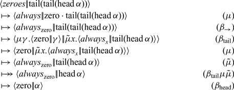
In contrast, notice how the same calculation in call-by-name builds up a delayed computation in the seed:
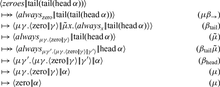
Consider the function that produces a stream that counts down from some initial number n to 0, and then staying at 0. Informally, this function can be understood as:
 \begin{align*} \mathit{countDown} &: \operatorname{Nat} \to \operatorname{Stream} \operatorname{Nat} \\ \mathit{countDown}~n &= n, n-1, n-2, \dots, 3, 2, 1, 0, 0, 0, \dots\end{align*}
which corresponds to the Haskell function
 \begin{align*} \mathit{countDown}~0 &= \mathit{zeroes} \\ \mathit{countDown}~n &= n : \mathit{countDown}~(n-1)\end{align*}
It is formally defined in the abstract machine like so:
 \begin{align*}\begin{aligned}[t] \textit{countDown} \ n = \operatorname{\mathbf{corec}}{} \{& \operatorname{head} \alpha \to \alpha \\ \mid& \operatorname{tail} \_ \to \gamma. \begin{aligned}[t] \operatorname{\mathbf{rec}}{} \{& \operatorname{zero} \to \operatorname{zero} \\ \mid& \operatorname{succ} n \to n \} \operatorname{\mathbf{with}} \gamma \} \end{aligned} \\ \operatorname{\mathbf{with}}{}& n\end{aligned}\end{align*}
This definition of $\mathit{countDown}$
can be understood as follows:
$\mathit{countDown}$
can be understood as follows:
If the head of the stream is requested (matching the copattern
$\operatorname{head}\alpha$
), then the current value x of the seed is returned (to
$\alpha$
) as-is.Otherwise, if the tail is requested (matching the copattern
$\operatorname{tail}\_$
), then the current value of the seed is inspected: if it is 0, then 0 is used again as the seed; otherwise, the seed is the successor of some y, in which case y is given as the updated seed.


The previous definition of $\mathit{countDown}$
is not very efficient; once n reaches zero, one can safely returns the zeroes stream thus avoiding the test for each question. This can be avoided with the power of the corecursor as so:
$\mathit{countDown}$
is not very efficient; once n reaches zero, one can safely returns the zeroes stream thus avoiding the test for each question. This can be avoided with the power of the corecursor as so:
 \begin{align*}\begin{aligned}[t] \mathit{countDown'} \ n = \operatorname{\mathbf{corec}}{} \{& \operatorname{head} \alpha \to \alpha \\ \mid& \operatorname{tail} \beta \to \gamma. \begin{aligned}[t] \operatorname{\mathbf{rec}}{} \{& \operatorname{zero} \to \mu{\_}. \langle {\mathit{zeroes}} |\!| {\beta} \rangle \\ \mid& \operatorname{succ} n \to \gamma. n \} \operatorname{\mathbf{with}} \gamma \} \end{aligned} \\ \operatorname{\mathbf{with}}{}& n\end{aligned}\end{align*}
Note that in the coinductive step, the decision on which continuation is taken (the observer of the tail $\beta$
or the continuation of corecursion
$\beta$
or the continuation of corecursion $\gamma$
) depends on the current value of the seed. If the seed reaches 0 the corecursion is stopped and the stream of zeros is returned instead.
$\gamma$
) depends on the current value of the seed. If the seed reaches 0 the corecursion is stopped and the stream of zeros is returned instead.
Another example of this “switching” behavior, where one corecursive loop (like $\mathit{countDown'}~0$
) ends and switches to another corecursive loop (like
$\mathit{countDown'}~0$
) ends and switches to another corecursive loop (like $\mathit{zeroes}$
) is the
$\mathit{zeroes}$
) is the $\mathit{switch0}$
function informally written as
$\mathit{switch0}$
function informally written as
 \begin{align*} \mathit{switch0}~(x_0,x_1,\dots,0,x_{i+1},\dots)~(y_0,y_1,\dots) &= x_0, x_1, \dots, 0, y_0, y_1, \dots &(\text{if } \forall j < i. x_j \neq 0) \\ \mathit{switch0}~(x_0,x_1,\dots)~(y_0,y_1,\dots) &= x_0, x_1, \dots &(\text{if } \forall j. x_j \neq 0)\end{align*}
which corresponds to the Haskell code:
 \begin{align*} \mathit{switch0}~(0:xs)~ys &= 0 : ys \\ \mathit{switch0}~(x:xs)~ys &= x : \mathit{switch0}~xs~ys\end{align*}
Intuitively, $\mathit{switch0}~xs~ys$
will generate the stream produced by xs until a 0 is reached; at that point, the
$\mathit{switch0}~xs~ys$
will generate the stream produced by xs until a 0 is reached; at that point, the $\mathit{switch0}$
loop ends by returning 0 followed by the whole stream ys as-is. This example is more interesting than
$\mathit{switch0}$
loop ends by returning 0 followed by the whole stream ys as-is. This example is more interesting than $\mathit{countDown}$
because there is no inductive argument (like a number or a list) that the function can inspect in advance to predict when the switch will occur. Instead,
$\mathit{countDown}$
because there is no inductive argument (like a number or a list) that the function can inspect in advance to predict when the switch will occur. Instead, $\mathit{switch0}$
must generate its elements on demand only when they are requested, and the switch to ys will only happen if an observer decides to look deep enough into the stream to hit an 0 inside xs, which might never even happen.
$\mathit{switch0}$
must generate its elements on demand only when they are requested, and the switch to ys will only happen if an observer decides to look deep enough into the stream to hit an 0 inside xs, which might never even happen. $\mathit{switch0}$
can be efficiently implemented in the abstract machine using both continuations provided by the corecursor like so:
$\mathit{switch0}$
can be efficiently implemented in the abstract machine using both continuations provided by the corecursor like so:
 \begin{align*} \mathit{switch0}~xs~ys = \operatorname{\mathbf{corec}} &\{ \operatorname{head} \alpha \to \alpha \\ &\mid \operatorname{tail} \beta \to \gamma. {\tilde{\mu}}{xs}. \langle {xs} |\!| { \operatorname{head} \begin{aligned}[t] \operatorname{\mathbf{rec}} &\{ \operatorname{zero} \to ys \\ &\mid \operatorname{succ} n \to \mu{\_}.\langle {xs} |\!| {\operatorname{tail} \gamma} \rangle \} \\ &\operatorname{\mathbf{with}} \beta \rangle \} \end{aligned} } \\ &\operatorname{\mathbf{with}} xs\end{align*}
The internal state to this corecursive loop contains the remainder of xs that hasn’t been seen yet. While the $\mathit{switch0}$ $\operatorname{\mathbf{corec}}$
loop is active, it will always generate the
$\operatorname{\mathbf{corec}}$
loop is active, it will always generate the $\operatorname{head}$
of the current remainder of xs as its own
$\operatorname{head}$
of the current remainder of xs as its own $\operatorname{head}$
element. When the
$\operatorname{head}$
element. When the $\operatorname{tail}$
is requested, this loop checks the
$\operatorname{tail}$
is requested, this loop checks the $\operatorname{head}$
of the xs remainder to decide what to do:
$\operatorname{head}$
of the xs remainder to decide what to do:
if it is
$\operatorname{zero}$
, then the whole stream ys gets returned to
$\beta$
, which is the original caller who requested the
$\operatorname{tail}$
of the stream, otherwiseif it is
$\operatorname{succ} n$
, the
$\operatorname{\mathbf{corec}}$
loop inside
$\mathit{switch0}$
will continue by returning the
$\operatorname{tail}$
of the remaining xs to the continuation
$\gamma$
which will update the internal state of the loop with one fewer element that has not yet been seen.


4.2 Properly de Morgan Dual (co)recursive types
Although we derived corecursion from recursion using duality, our prototypical examples of natural numbers and streams were not perfectly dual to one another. While the (co)recursive case of $\operatorname{tail} E$
looks similar enough to
$\operatorname{tail} E$
looks similar enough to $\operatorname{succ} V$
, the base cases of
$\operatorname{succ} V$
, the base cases of $\operatorname{head} E$
and
$\operatorname{head} E$
and $\operatorname{zero}$
don’t exactly line up, because
$\operatorname{zero}$
don’t exactly line up, because $\operatorname{head}$
takes a parameter but
$\operatorname{head}$
takes a parameter but $\operatorname{zero}$
does not.
$\operatorname{zero}$
does not.
One way to perfect the duality is to generalize $\operatorname{Nat}$
to
$\operatorname{Nat}$
to $\operatorname{Numbered} A$
which represents a value of type A labeled with a natural number (also known as Burroni naturals).
$\operatorname{Numbered} A$
which represents a value of type A labeled with a natural number (also known as Burroni naturals). $\operatorname{Numbered} A$
has two constructors: the base case
$\operatorname{Numbered} A$
has two constructors: the base case $\operatorname{zero} : A \to \operatorname{Numbered} A$
labels an A value with the number 0, and
$\operatorname{zero} : A \to \operatorname{Numbered} A$
labels an A value with the number 0, and $\operatorname{succ} : \operatorname{Numbered} A \to \operatorname{Numbered} A$
increments the numeric label while leaving the A value alone, as shown by the following rules:
$\operatorname{succ} : \operatorname{Numbered} A \to \operatorname{Numbered} A$
increments the numeric label while leaving the A value alone, as shown by the following rules:
In order to match the generalized $\operatorname{zero}$
constructor, the base case of the recursor needs to be likewise generalized with an extra parameter. In System T, this looks like
$\operatorname{zero}$
constructor, the base case of the recursor needs to be likewise generalized with an extra parameter. In System T, this looks like
 \begin{align*} \operatorname{\mathbf{rec}} M \operatorname{\mathbf{as}}{} \{\operatorname{zero} x \to N \mid \operatorname{succ} y \to z.N'\} ,\end{align*}
while in the abstract machine we get the generalized continuation
\begin{align*} \operatorname{\mathbf{rec}} M \operatorname{\mathbf{as}}{} \{\operatorname{zero} x \to N \mid \operatorname{succ} y \to z.N'\} ,\end{align*}
while in the abstract machine we get the generalized continuation
 \begin{align*} \operatorname{\mathbf{rec}}{} \{\operatorname{zero} x \to v \mid \operatorname{succ} y \to z.w\} \operatorname{\mathbf{with}} E .\end{align*}
The typing rule for this continuation is:
\begin{align*} \operatorname{\mathbf{rec}}{} \{\operatorname{zero} x \to v \mid \operatorname{succ} y \to z.w\} \operatorname{\mathbf{with}} E .\end{align*}
The typing rule for this continuation is:
It turns out that $\operatorname{Numbered} A$
is the proper de Morgan dual to
$\operatorname{Numbered} A$
is the proper de Morgan dual to $\operatorname{Stream} A$
. Notice how the two constructors
$\operatorname{Stream} A$
. Notice how the two constructors $\operatorname{zero} V$
and
$\operatorname{zero} V$
and $\operatorname{succ} W$
exactly mirror the two destructors
$\operatorname{succ} W$
exactly mirror the two destructors $\operatorname{head} E$
and
$\operatorname{head} E$
and $\operatorname{tail} F$
when we swap the roles of values and covalues. The recursor continuation of the form
$\operatorname{tail} F$
when we swap the roles of values and covalues. The recursor continuation of the form
 \begin{align*} \operatorname{\mathbf{rec}}{} \{\operatorname{zero} x \to v \mid \operatorname{succ} y \to z.w\} \operatorname{\mathbf{with}} E\end{align*}
is the perfect mirror image of the stream corecursor
\begin{align*} \operatorname{\mathbf{rec}}{} \{\operatorname{zero} x \to v \mid \operatorname{succ} y \to z.w\} \operatorname{\mathbf{with}} E\end{align*}
is the perfect mirror image of the stream corecursor
 \begin{align*} \operatorname{\mathbf{corec}}{} \{\operatorname{head}\alpha \to e \mid \operatorname{tail}\beta \to \gamma.f\} \operatorname{\mathbf{with}} V\end{align*}
when we likewise swap variables with covariables in the (co)patterns. In more detail, we can write the duality relation between values and covalues as
\begin{align*} \operatorname{\mathbf{corec}}{} \{\operatorname{head}\alpha \to e \mid \operatorname{tail}\beta \to \gamma.f\} \operatorname{\mathbf{with}} V\end{align*}
when we likewise swap variables with covariables in the (co)patterns. In more detail, we can write the duality relation between values and covalues as $\mathrel{\overline\sim}$
. Assuming that
$\mathrel{\overline\sim}$
. Assuming that $V \mathrel{\overline\sim} E$
, we have the following duality between the constructors and destructors of these two types:
$V \mathrel{\overline\sim} E$
, we have the following duality between the constructors and destructors of these two types:
 \begin{align*} \operatorname{zero} V &\mathrel{\overline\sim} \operatorname{head} E & \operatorname{succ} V &\mathrel{\overline\sim} \operatorname{tail} E\end{align*}
For (co)recursion, we have the following dualities, assuming $v \mathrel{\overline\sim} e$
(under
$v \mathrel{\overline\sim} e$
(under $x \mathrel{\overline\sim} \alpha$
)
$x \mathrel{\overline\sim} \alpha$
) $w \mathrel{\overline\sim} f$
(under
$w \mathrel{\overline\sim} f$
(under $y \mathrel{\overline\sim} \beta$
and
$y \mathrel{\overline\sim} \beta$
and $z \mathrel{\overline\sim} \gamma$
), and
$z \mathrel{\overline\sim} \gamma$
), and $V \mathrel{\overline\sim} E$
:
$V \mathrel{\overline\sim} E$
:
 \begin{align*} \operatorname{\mathbf{corec}} \{\operatorname{head} \alpha \to e \mid \operatorname{tail} \beta \to \gamma. f\} \operatorname{\mathbf{with}} V &\mathrel{\overline\sim} \operatorname{\mathbf{rec}} \{\operatorname{zero} x \to v \mid \operatorname{succ} y \to z.w\} \operatorname{\mathbf{with}} E\end{align*}
We could also express the proper de Morgan duality by restricting streams instead of generalizing numbers. In terms of the type defined above, $\operatorname{Nat}$
is isomorphic to
$\operatorname{Nat}$
is isomorphic to $\operatorname{Numbered} \top$
, where
$\operatorname{Numbered} \top$
, where $\top$
represents the usual unit type with a single value (often written as ()). Since
$\top$
represents the usual unit type with a single value (often written as ()). Since $\top$
corresponds to logical truth, its dual is the
$\top$
corresponds to logical truth, its dual is the $\bot$
type corresponding to logical falsehood with no (closed) values, and a single covalue that represents an empty continuation. With this in mind, the type
$\bot$
type corresponding to logical falsehood with no (closed) values, and a single covalue that represents an empty continuation. With this in mind, the type $\operatorname{Nat}$
is properly dual to
$\operatorname{Nat}$
is properly dual to $\operatorname{Stream} \bot$
, i.e., an infinite stream of computations which cannot return any value to their observer.
Footnote 8
$\operatorname{Stream} \bot$
, i.e., an infinite stream of computations which cannot return any value to their observer.
Footnote 8
In order to fully realize this de Morgan duality in an interesting way that can talk about functions, we need to refer to the duals of those functions. Logically, the dual to the function type $A \to B$
(classical equivalent to
$A \to B$
(classical equivalent to $(\neg A) \vee B$
and
$(\neg A) \vee B$
and $\neg (A \wedge (\neg B))$
, whose continuations
$\neg (A \wedge (\neg B))$
, whose continuations $V \cdot E $
contain an argument V of type A paired with a consumer E of Bs) is a subtraction type
$V \cdot E $
contain an argument V of type A paired with a consumer E of Bs) is a subtraction type $B - A$
(classically equivalent to
$B - A$
(classically equivalent to $B \wedge (\neg A)$
for typing a pair
$B \wedge (\neg A)$
for typing a pair $E \cdot V$
of a value V of type B and a continuation E expecting As). Following (Curien & Herbelin, 2000), this subtraction type, along with the units
$E \cdot V$
of a value V of type B and a continuation E expecting As). Following (Curien & Herbelin, 2000), this subtraction type, along with the units $\top$
and
$\top$
and $\bot$
, can be added to our uniform abstract machine with the following extended syntax of (co)values, reduction rule
$\bot$
, can be added to our uniform abstract machine with the following extended syntax of (co)values, reduction rule $\beta_-$
for when a subtraction pair
$\beta_-$
for when a subtraction pair $E \cdot V$
interacts with the continuation abstraction
$E \cdot V$
interacts with the continuation abstraction $\tilde{\lambda} \alpha e$
, and typing rules:
$\tilde{\lambda} \alpha e$
, and typing rules:

Extending the uniform abstract machine with these new rules, lets us formally define a de Morgan duality transformation, shown in Fig. 9, that converts any term v producing type A into the coterm $v^\bot$
consuming type
$v^\bot$
consuming type $A^\bot$
, converts any coterm e expecting type A to a term
$A^\bot$
, converts any coterm e expecting type A to a term $e^\bot$
giving type
$e^\bot$
giving type $A^\bot$
, and converts a command c to its dual command
$A^\bot$
, and converts a command c to its dual command $c^\bot$
. The duality transformation assumes a bijection between variables and covariables (so that
$c^\bot$
. The duality transformation assumes a bijection between variables and covariables (so that $x^\bot$
denotes a unique covariable
$x^\bot$
denotes a unique covariable $\alpha$
such that
$\alpha$
such that $\alpha^\bot = x$
, and vice versa), which makes the whole transformation involutive (e.g.,
$\alpha^\bot = x$
, and vice versa), which makes the whole transformation involutive (e.g., $c^{\bot\bot} = c$
and
$c^{\bot\bot} = c$
and $A^{\bot\bot} = A$
) by definition. This generalizes the previous duality theorems for the classical sequent calculus (Curien & Herbelin, 2000; Wadler, Reference Wadler2003)—namely that involutive duality inverts typing and operational semantics in a meaningful way—to also incorporate (co)recursion on numbers and streams.
$A^{\bot\bot} = A$
) by definition. This generalizes the previous duality theorems for the classical sequent calculus (Curien & Herbelin, 2000; Wadler, Reference Wadler2003)—namely that involutive duality inverts typing and operational semantics in a meaningful way—to also incorporate (co)recursion on numbers and streams.
Duality of types, (co)terms, and commands in the uniform abstract machine.

Theorem 4.2 (Duality) In the fully dual abstract machine (the uniform abstract machine extended with subtraction $A - B$
and units
$A - B$
and units $\top$
and
$\top$
and $\bot$
), the following symmetries hold:
$\bot$
), the following symmetries hold:
-
1.
$\Gamma \vdash v : A$
is derivable if and only if
$\Gamma^\bot \vdash v^\bot \div A^\bot$
is.
-
2.
$\Gamma \vdash c \ $
is derivable if and only if
$\Gamma^\bot \vdash c^\bot \ $
is.
-
3. v is a call-by-value value if and only if
$e^\bot$
is a call-by-name covalue.
-
4.
$c \mapsto c'$
in call-by-name if and only if
$c^\bot \mapsto c'^\bot$
in call-by-value.


The proof of Theorem 4.2 just follows by induction on the given typing derivation or reduction rule and is an application of the duality theorem of general data and codata types (Downen, 2017), extended with the new form of primitive (co)recursor.
Intermezzo 4.3 The reader already familiar with other work on streams and duality, who has heard that finite lists are “dual” to (possibly) infinite streams, might be surprised to see the statement in Fig. 9 and Theorem 4.2 that streams are dual to (a generalization of) natural numbers. How can this be? The conflict is in two different meanings of the word “dual.”
The meaning of “dual” we use here corresponds exactly to the usual notion of de Morgan duality from classical logic. De Morgan duality flips between “true” ( $\top$
) and “false” (
$\top$
) and “false” ( $\bot$
), and between “and” (
$\bot$
), and between “and” ( $A \times B$
) and “or” (
$A \times B$
) and “or” ( $A + B$
), so that the dual of a proposition A is
$A + B$
), so that the dual of a proposition A is $A^\bot$
(logically equivalent to
$A^\bot$
(logically equivalent to $\neg A$
) defined like so:
$\neg A$
) defined like so:
 \begin{align*} \top^\bot &:= \bot & \bot^\bot &:= \top & (A + B)^\bot &:= (A^\bot) \times (B^\bot) & (A \times B)^\bot &:= (A^\bot) + (B^\bot) \end{align*}
Importantly, notice how the duality transformation is deep: $A^\bot$
does not just flip the top connective, it flips all the connectives down to the leaves. For example, the proposition dual to
$A^\bot$
does not just flip the top connective, it flips all the connectives down to the leaves. For example, the proposition dual to $(\top + \bot) \times \top$
(which is tautologically true) is
$(\top + \bot) \times \top$
(which is tautologically true) is
 \begin{align*} ((\top + \bot) \times \top)^\bot = (\bot \times \top) + \bot \end{align*}
(which denotes a falsehood, the dual to truth) and not the erroneous illogical inequality
\begin{align*} ((\top + \bot) \times \top)^\bot = (\bot \times \top) + \bot \end{align*}
(which denotes a falsehood, the dual to truth) and not the erroneous illogical inequality
 \begin{align*} ((\top + \bot) \times \top)^\bot \neq (\top + \bot) + \top \end{align*}
(which still tautology true, and not the dual).
\begin{align*} ((\top + \bot) \times \top)^\bot \neq (\top + \bot) + \top \end{align*}
(which still tautology true, and not the dual).
Previous (Curien & Herbelin, 2000; Wadler, Reference Wadler2003) has showed how this duality of propositions in a logic can naturally extend to a duality of types in a programming language based on the classical sequent calculus. Because we are interested in (co)inductive types here, we also need to consider how this relates to recursion in types. As usual, inductive types like $\operatorname{Nat}$
are modeled as a least fixed point, that we write as
$\operatorname{Nat}$
are modeled as a least fixed point, that we write as $\operatorname{LFP} X. A$
, whereas coinductive types like
$\operatorname{LFP} X. A$
, whereas coinductive types like $\operatorname{Stream} A$
are modeled as a greatest fixed point, that we write as
$\operatorname{Stream} A$
are modeled as a greatest fixed point, that we write as $\operatorname{GFP} X. A$
.
Footnote 9
A key aspect of this paper is to effectively generalize the classical de Morgan duality of Curien & Herbelin (2000); Wadler (Reference Wadler2003) to the known dualities of least and greatest fixed points:
$\operatorname{GFP} X. A$
.
Footnote 9
A key aspect of this paper is to effectively generalize the classical de Morgan duality of Curien & Herbelin (2000); Wadler (Reference Wadler2003) to the known dualities of least and greatest fixed points:
 \begin{align*} (\operatorname{LFP} X. A)^\bot &:= \operatorname{GFP} X. (A^\bot) & (\operatorname{GFP} X. A)^\bot &:= \operatorname{LFP} X. (A^\bot) \end{align*}
The $\operatorname{Stream} A$
,
$\operatorname{Stream} A$
, $\operatorname{Nat}$
, and
$\operatorname{Nat}$
, and $\operatorname{Numbered} A$
types we have seen thus far are isomorphic (denoted as
$\operatorname{Numbered} A$
types we have seen thus far are isomorphic (denoted as $\approx$
) to these usual encodings in terms of greatest and least fixed points built on top of basic type constructors like
$\approx$
) to these usual encodings in terms of greatest and least fixed points built on top of basic type constructors like $+$
and
$+$
and $\times$
:
$\times$
:
 \begin{align*} \operatorname{Stream} A &\approx \operatorname{GFP} X.~ A \times X & \operatorname{Nat} &\approx \operatorname{LFP} X.~ \top + X & \operatorname{Numbered} A &\approx \operatorname{LFP} X.~ A + X \end{align*}
By applying the usual de Morgan duality of classical logic along with the duality of greatest and least fixed points above, we can calculate these duals of streams and natural numbers:
 \begin{align*} (\operatorname{Stream} A)^\bot &\approx \operatorname{LFP} X.~ A^\bot + X \approx \operatorname{Numbered} (A^\bot) & \operatorname{Nat}^\bot &\approx \operatorname{GFP} X.~ \bot \times X \approx \operatorname{Stream} \bot \end{align*}
Contrastingly, other work on (co)inductive types instead calls two types “duals” by just flipping between the greatest or fixed point at the top of the top, but leaving everything else alone. In other words, this other literature says that the dual of $\operatorname{LFP} X. A$
is just
$\operatorname{LFP} X. A$
is just $\operatorname{GFP} X. A$
, instead of
$\operatorname{GFP} X. A$
, instead of $\operatorname{GFP} X. (A^\bot)$
. In comparison, this is a shallow notion of duality that does not look deeper into the type. The typical working example of this notion of duality is that the inductive type of lists (
$\operatorname{GFP} X. (A^\bot)$
. In comparison, this is a shallow notion of duality that does not look deeper into the type. The typical working example of this notion of duality is that the inductive type of lists ( $\operatorname{List} A$
) is dual to the coinductive type of possibly infinite or finite lists (InfList A), modeled like so:
$\operatorname{List} A$
) is dual to the coinductive type of possibly infinite or finite lists (InfList A), modeled like so:
 \begin{align*} \operatorname{List} A &\approx \operatorname{LFP} X. \top + (A \times X) & InfList A &\approx \operatorname{GFP} X. \top + (A \times X) \end{align*}
This other notion of duality, which only swaps a greatest for a list fixed point, is closest to the work on corecursion in lazy functional languages like Haskell, where InfList A represents Haskell’s usual list type [a]. The work has undoubtedly been very productive in showing how to solve practical programming problems involving infinite data in the context of lazy functional languages, but covers different ground than our main objective. For example, shallow duality that just swaps the top-most fixed point—and ignores the rest of the underlying type—fails at providing an involutive duality of types and computation like the one shown in Theorem 4.2 and Fig. 9. Intuitively, $(\operatorname{List} A)^\bot \neq$
InfList A because a finite list of As looks nothing like the continuation expecting a (possibly infinite) list of A, and vice versa!
$(\operatorname{List} A)^\bot \neq$
InfList A because a finite list of As looks nothing like the continuation expecting a (possibly infinite) list of A, and vice versa!
5 Corecursion versus coiteration: Expressiveness and efficiency
Similar to recursion, we can define two special cases of corecursion which only use part of its functionality by just ignoring a parameter in the corecursive branch. We derive the encodings for the creation of streams by applying the syntactic duality to the encodings presented in Section 3.5:
 \begin{align*}\begin{aligned} & \operatorname{\mathbf{cocase}} \\ &\quad \begin{alignedat}[t]{2} \{& \operatorname{head} \alpha &&\to e \\ \mid& \operatorname{tail} \beta &&\to f \} \end{alignedat} \\ &\operatorname{\mathbf{with}} V\end{aligned}&:=\!\!\begin{aligned} &\operatorname{\mathbf{corec}} \\ &\quad \begin{alignedat}[t]{2} \{& \operatorname{head} \alpha &&\to e \\ \mid& \operatorname{tail} \beta &&\to \rule{1ex}{0.5pt}\,. f \} \end{alignedat} \\ &\operatorname{\mathbf{with}} V\end{aligned}&\quad\begin{aligned} & \operatorname{\mathbf{coiter}} \\ &\quad \begin{alignedat}[t]{2} \{& \operatorname{head} \alpha &&\to e \\ \mid& \operatorname{tail} &&\to \gamma.f \} \end{alignedat} \\ &\operatorname{\mathbf{with}} V\end{aligned}&:=\!\!\begin{aligned} &\operatorname{\mathbf{corec}} \\ &\quad \begin{alignedat}[t]{2} \{& \operatorname{head} \alpha &&\to e \\ \mid& \operatorname{tail} \rule{1ex}{0.5pt} &&\to \gamma.f \} \end{alignedat} \\ &\operatorname{\mathbf{with}} V\end{aligned}\end{align*}
Specifically, $\operatorname{\mathbf{cocase}}$
simply matches on the shape of its projection, which has the form
$\operatorname{\mathbf{cocase}}$
simply matches on the shape of its projection, which has the form $\operatorname{head}\alpha$
or
$\operatorname{head}\alpha$
or $\operatorname{tail}\beta$
, without corecursing at all. In contrast,
$\operatorname{tail}\beta$
, without corecursing at all. In contrast, $\operatorname{\mathbf{coiter}}$
always corecurses by providing an updated accumulator in the
$\operatorname{\mathbf{coiter}}$
always corecurses by providing an updated accumulator in the $\operatorname{tail}\beta$
case without ever referring to
$\operatorname{tail}\beta$
case without ever referring to $\beta$
. We have seen already several examples of coiteration. Indeed, all examples given in the previous section, except
$\beta$
. We have seen already several examples of coiteration. Indeed, all examples given in the previous section, except $\mathit{countDown'}$
, are examples of coiteration, as indicated by the absence of the rest of the continuation (named
$\mathit{countDown'}$
, are examples of coiteration, as indicated by the absence of the rest of the continuation (named $\_$
). From the perspective of logic, coiteration can be seen as intuitionistic because it only ever involves one continuation (corresponding to one conclusion) at a time. In contrast, the most general form of the corecursor is inherently classical because the corecursive step
$\_$
). From the perspective of logic, coiteration can be seen as intuitionistic because it only ever involves one continuation (corresponding to one conclusion) at a time. In contrast, the most general form of the corecursor is inherently classical because the corecursive step $\operatorname{tail} \beta \to \gamma. f$
introduces two continuations
$\operatorname{tail} \beta \to \gamma. f$
introduces two continuations $\beta$
and
$\beta$
and $\gamma$
(corresponding to two different conclusion) at the same time.
$\gamma$
(corresponding to two different conclusion) at the same time.
Recall from Section 2 that recursion in call-by-name versus call-by-value have different algorithmic complexities. The same holds for corecursion, with the benefit going instead to call-by-value. Indeed, in call-by-value the simple cocase continuation avoids the corecursive step entirely in two steps:
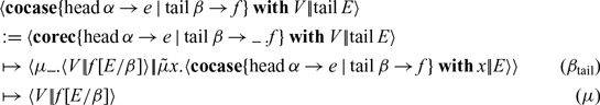
whereas cocase continues corecursing in call-by-name, despite the fact that this work will ultimately be thrown away once any element is requested via $\operatorname{head}$
:
$\operatorname{head}$
:

As an example of cocase, consider the following stream:
 \begin{align*} \mathit{scons}~x~(y_1,y_2,\dots) &= x, y_1, y_2, \dots\end{align*} $\mathit{scons}~x~s$
appends a new element x on top of the stream s. This informal definition can be formalized in terms of
$\mathit{scons}~x~s$
appends a new element x on top of the stream s. This informal definition can be formalized in terms of $\operatorname{\mathbf{cocase}}$
like so:
$\operatorname{\mathbf{cocase}}$
like so:
 \begin{align*} \mathit{scons} &:= \lambda x. \lambda s. \operatorname{\mathbf{cocase}} \{ \operatorname{head} \alpha \to \alpha \mid \operatorname{tail} \beta \to {\tilde{\mu}}{\_}. \langle {s} |\!| {\beta} \rangle \} \operatorname{\mathbf{with}} x \end{align*}
Ideally, $\mathit{scons}$
should not leave a lingering effect on the underlying stream. That is to say, the tail of
$\mathit{scons}$
should not leave a lingering effect on the underlying stream. That is to say, the tail of $\mathit{scons}~x~s$
should just be s. This happens directly in call-by-value. Consider indexing the
$\mathit{scons}~x~s$
should just be s. This happens directly in call-by-value. Consider indexing the $n+1^{th}$
element of
$n+1^{th}$
element of $\mathit{scons}$
in call-by-value, where we write
$\mathit{scons}$
in call-by-value, where we write $\operatorname{tail}^n E$
to mean the n-fold application of
$\operatorname{tail}^n E$
to mean the n-fold application of $\operatorname{tail}$
over E (i.e.,
$\operatorname{tail}$
over E (i.e., $\operatorname{tail}^0 E = E$
and
$\operatorname{tail}^0 E = E$
and $\operatorname{tail}^{n+1} E = \operatorname{tail}(\operatorname{tail}^n E)$
):
$\operatorname{tail}^{n+1} E = \operatorname{tail}(\operatorname{tail}^n E)$
):

Notice how, after the first $\operatorname{tail}$
is resolved, the computation incurred by
$\operatorname{tail}$
is resolved, the computation incurred by $\mathit{scons}$
has completely vanished. In contrast, the computation of
$\mathit{scons}$
has completely vanished. In contrast, the computation of $\mathit{scons}$
continues to linger in call-by-name:
$\mathit{scons}$
continues to linger in call-by-name:

Here, we will spend time over the next n $\operatorname{tail}$
projections to build up an ever larger accumulator until the
$\operatorname{tail}$
projections to build up an ever larger accumulator until the $\operatorname{head}$
is reached, even though the result will inevitably just backtrack to directly ask s for
$\operatorname{head}$
is reached, even though the result will inevitably just backtrack to directly ask s for $\operatorname{tail}^n E$
.
$\operatorname{tail}^n E$
.
However, one question remains: how do we accurately measure the cost of a stream? The answer is more subtle than the cost of numeric loops, because streams more closely resemble functions. With functions, it is not good enough to just count the steps it takes to calculate the closure. We also need to count the steps taken in the body of the function when it is called, i.e., what happens when the function is used. The same issue occurs with streams, where we also need to count what happens when the stream is used, i.e., the number of steps taken inside the stream in response to a projection. Of course, the internal number of steps in both cases can depend on the “size” of the input. For functions, this is the size of its argument; in the simple case of $\operatorname{Nat} \to \operatorname{Nat}$
, this size is just the value n of the numeric argument
$\operatorname{Nat} \to \operatorname{Nat}$
, this size is just the value n of the numeric argument $\operatorname{succ}^n\operatorname{zero}$
itself. For streams, the input is the stream projection of the form
$\operatorname{succ}^n\operatorname{zero}$
itself. For streams, the input is the stream projection of the form $\operatorname{tail}^n(\operatorname{head}\alpha)$
, whose size is proportional to the number n of
$\operatorname{tail}^n(\operatorname{head}\alpha)$
, whose size is proportional to the number n of $\operatorname{tail}$
projections. Therefore, the computational complexity of a stream value s—perhaps defined by a
$\operatorname{tail}$
projections. Therefore, the computational complexity of a stream value s—perhaps defined by a $\operatorname{\mathbf{corec}}$
term—is expressed as some O(f(n)), where n denotes the depth of the projection given by the number of
$\operatorname{\mathbf{corec}}$
term—is expressed as some O(f(n)), where n denotes the depth of the projection given by the number of $\operatorname{tail}$
s.
$\operatorname{tail}$
s.
Now, let us consider the asymptotic cost of $\mathit{scons}$
under both call-by-value and call-by-name evaluation. In general, the difference in performance between
$\mathit{scons}$
under both call-by-value and call-by-name evaluation. In general, the difference in performance between $\langle {\mathit{scons}} |\!| {x \cdot s \cdot E} \rangle$
and
$\langle {\mathit{scons}} |\!| {x \cdot s \cdot E} \rangle$
and $\langle {s} |\!| {E} \rangle$
in call-by-value is just a constant time (O(1)) overhead. So, given that the cost of s is O(f(n)), then the cost of
$\langle {s} |\!| {E} \rangle$
in call-by-value is just a constant time (O(1)) overhead. So, given that the cost of s is O(f(n)), then the cost of $\langle {\mathit{scons}} |\!| {x \cdot s \cdot E} \rangle$
will also be O(f(n)). In contrast, the call-by-name evaluation of
$\langle {\mathit{scons}} |\!| {x \cdot s \cdot E} \rangle$
will also be O(f(n)). In contrast, the call-by-name evaluation of $\mathit{scons}$
incurs an additional linear time (O(n)) overhead based on depth of the projection:
$\mathit{scons}$
incurs an additional linear time (O(n)) overhead based on depth of the projection: $\langle {\mathit{scons}} |\!| {x \cdot s \cdot \operatorname{tail}^{n+1}(\operatorname{head} E)} \rangle$
takes an additional number of steps proportional to n compared to the cost of executing
$\langle {\mathit{scons}} |\!| {x \cdot s \cdot \operatorname{tail}^{n+1}(\operatorname{head} E)} \rangle$
takes an additional number of steps proportional to n compared to the cost of executing $\langle {s} |\!| {\operatorname{tail}^n(\operatorname{head} E)} \rangle$
. As a consequence, the call-by-name cost of
$\langle {s} |\!| {\operatorname{tail}^n(\operatorname{head} E)} \rangle$
. As a consequence, the call-by-name cost of $\langle {\mathit{scons}} |\!| {x \cdot s \cdot E} \rangle$
is
$\langle {\mathit{scons}} |\!| {x \cdot s \cdot E} \rangle$
is $O(n+f(n))$
, given that the cost of s is O(f(n)). So the efficiency of corecursion is better in call-by-value than in call-by-name.
$O(n+f(n))$
, given that the cost of s is O(f(n)). So the efficiency of corecursion is better in call-by-value than in call-by-name.
To make the analysis more concrete, let’s look at an application of $\mathit{scons}$
to a specific underlying stream. Recall the
$\mathit{scons}$
to a specific underlying stream. Recall the $\mathit{countDown}$
function from Section 4.1 which produces a stream counting down from a given n:
$\mathit{countDown}$
function from Section 4.1 which produces a stream counting down from a given n: $n, n-1, \dots, 2, 1, 0, 0, \dots$
. This function (and the similar
$n, n-1, \dots, 2, 1, 0, 0, \dots$
. This function (and the similar $\mathit{countDown'}$
) is defined to immediately return a stream value that captures the starting number n, and then incrementally counts down one at a time with each
$\mathit{countDown'}$
) is defined to immediately return a stream value that captures the starting number n, and then incrementally counts down one at a time with each $\operatorname{tail}$
projection. An alternative method of generating this same stream is to do all the counting up-front: recurse right away on the starting number and use
$\operatorname{tail}$
projection. An alternative method of generating this same stream is to do all the counting up-front: recurse right away on the starting number and use $\mathit{scons}$
to piece together the stream from each step towards zero. This algorithm can be expressed in terms of System T-style recursion like so:
$\mathit{scons}$
to piece together the stream from each step towards zero. This algorithm can be expressed in terms of System T-style recursion like so:
 \begin{align*} \mathit{countNow} \ n = \operatorname{\mathbf{rec}} n \operatorname{\mathbf{as}}{} \{& \operatorname{zero} \to \mathit{zeroes} \\ \mid& \operatorname{succ} x \to xs.~ \mathit{scons}~(\operatorname{succ} x)~xs \}\end{align*}
So that the translation of $\mathit{countNow}$
to the abstract machine language is:
$\mathit{countNow}$
to the abstract machine language is:

What is the cost of $\mathit{countNow}$
? First, the up-front cost of calling the function with the argument
$\mathit{countNow}$
? First, the up-front cost of calling the function with the argument $\operatorname{succ}^n\operatorname{zero}$
is unsurprisingly O(n), due to the use of the recursor. But this doesn’t capture the full cost; what is the efficiency of using the stream value returned by
$\operatorname{succ}^n\operatorname{zero}$
is unsurprisingly O(n), due to the use of the recursor. But this doesn’t capture the full cost; what is the efficiency of using the stream value returned by $\mathit{countNow}$
? To understand the efficiency of the stream, we have to consider both the initial numeric argument as well as the depth of the projection:
$\mathit{countNow}$
? To understand the efficiency of the stream, we have to consider both the initial numeric argument as well as the depth of the projection:
in the abstract machine language, which corresponds to $\operatorname{head}(\operatorname{tail}^m(\mathit{countNow}~(\operatorname{succ}^n\operatorname{zero})))$
in a functional style. In the base case, we have the stream
$\operatorname{head}(\operatorname{tail}^m(\mathit{countNow}~(\operatorname{succ}^n\operatorname{zero})))$
in a functional style. In the base case, we have the stream $\mathit{zeroes}$
, whose cost is O(m) because it must traverse past all m
$\mathit{zeroes}$
, whose cost is O(m) because it must traverse past all m $\operatorname{tail}$
projections before it can return a 0 to the
$\operatorname{tail}$
projections before it can return a 0 to the $\operatorname{head}$
projection. On top of this, we apply n applications of
$\operatorname{head}$
projection. On top of this, we apply n applications of $\mathit{scons}$
. Recall that in call-by-value, we said that the cost of
$\mathit{scons}$
. Recall that in call-by-value, we said that the cost of $\mathit{scons}$
is the same as the underlying stream. Thus, the call-by-value efficiency of the stream returned by
$\mathit{scons}$
is the same as the underlying stream. Thus, the call-by-value efficiency of the stream returned by $\langle {\mathit{countNow}} |\!| {\operatorname{succ}^n\operatorname{zero} \cdot \operatorname{tail}^m(\operatorname{head}\alpha)} \rangle$
is just O(m). In call-by-name in contrast,
$\langle {\mathit{countNow}} |\!| {\operatorname{succ}^n\operatorname{zero} \cdot \operatorname{tail}^m(\operatorname{head}\alpha)} \rangle$
is just O(m). In call-by-name in contrast, $\mathit{scons}$
adds an additional linear time overhead to the underlying stream. Since there are n applications of
$\mathit{scons}$
adds an additional linear time overhead to the underlying stream. Since there are n applications of $\mathit{scons}$
and the projection is m elements deep, the call-by-name efficiency of the stream returned by
$\mathit{scons}$
and the projection is m elements deep, the call-by-name efficiency of the stream returned by $\langle {\mathit{countNow}} |\!| {\operatorname{succ}^n\operatorname{zero} \cdot \operatorname{tail}^m(\operatorname{head}\alpha)} \rangle$
is
$\langle {\mathit{countNow}} |\!| {\operatorname{succ}^n\operatorname{zero} \cdot \operatorname{tail}^m(\operatorname{head}\alpha)} \rangle$
is $O(m(n+1))$
. If the count n and depth m are roughly proportional to each other (so that
$O(m(n+1))$
. If the count n and depth m are roughly proportional to each other (so that $n \approx m$
), the difference between call-by-value and call-by-name evaluation of
$n \approx m$
), the difference between call-by-value and call-by-name evaluation of $\mathit{countNow}$
’s stream is a jump between a linear time and quadratic time computation.
$\mathit{countNow}$
’s stream is a jump between a linear time and quadratic time computation.
5.1 Corecursion in terms of coiteration
Recall in Section 3.5 that we were able to encode $\operatorname{\mathbf{rec}}$
in terms of
$\operatorname{\mathbf{rec}}$
in terms of $\operatorname{\mathbf{iter}}$
, though at an increased computational cost. Applying syntactic duality, we can write a similar encoding of
$\operatorname{\mathbf{iter}}$
, though at an increased computational cost. Applying syntactic duality, we can write a similar encoding of $\operatorname{\mathbf{corec}}$
as a macro-expansion in terms of
$\operatorname{\mathbf{corec}}$
as a macro-expansion in terms of $\operatorname{\mathbf{coiter}}$
. Doing so requires the dual of pairs: sum types. Sum types in the abstract machine look like (Wadler, Reference Wadler2003):
$\operatorname{\mathbf{coiter}}$
. Doing so requires the dual of pairs: sum types. Sum types in the abstract machine look like (Wadler, Reference Wadler2003):
 \begin{align*} \langle {\operatorname{left} V} |\!| {[e_1,e_2]} \rangle &\mapsto \langle {V} |\!| {e_1} \rangle & \langle {\operatorname{right} V} |\!| {[e_1,e_2]} \rangle &\mapsto \langle {V} |\!| {e_2} \rangle &(\beta_+)\end{align*}
The macro-expansion for encoding $\operatorname{\mathbf{corec}}$
as
$\operatorname{\mathbf{corec}}$
as $\operatorname{\mathbf{coiter}}$
derived from duality is:
$\operatorname{\mathbf{coiter}}$
derived from duality is:
 \begin{align*}\begin{aligned} & \operatorname{\mathbf{corec}} \begin{alignedat}[t]{2} \{& \operatorname{head} \alpha &&\to e \\ \mid& \operatorname{tail} \beta &&\to \gamma.f \} \end{alignedat} \\ & \operatorname{\mathbf{with}} V\end{aligned}&:=\begin{aligned} &\operatorname{\mathbf{coiter}} \begin{alignedat}[t]{2} \{& \operatorname{head} \alpha &&\to [\operatorname{head}\alpha, e] \\ \mid& \operatorname{tail} &&\to [\beta, \gamma].[\operatorname{tail}\beta, f] \} \end{alignedat} \\ & \operatorname{\mathbf{with}}{} \operatorname{right} V\end{aligned}\end{align*}
Note how the coinductive step of $\operatorname{\mathbf{coiter}}$
has access to both an option to update the internal seed, or to return some other, fully formed stream as its tail. So dually to the encoding of the recursor, this encoding keeps both options open by reconstructing the original continuation alongside the continuation which uses its internal seed. In the base case matching
$\operatorname{\mathbf{coiter}}$
has access to both an option to update the internal seed, or to return some other, fully formed stream as its tail. So dually to the encoding of the recursor, this encoding keeps both options open by reconstructing the original continuation alongside the continuation which uses its internal seed. In the base case matching $\operatorname{head}\alpha$
, it rebuilds the observation
$\operatorname{head}\alpha$
, it rebuilds the observation $\operatorname{head}\alpha$
and pairs it up with the original response e to the base case. In the coinductive case matching
$\operatorname{head}\alpha$
and pairs it up with the original response e to the base case. In the coinductive case matching $\operatorname{tail}\beta$
, the projection
$\operatorname{tail}\beta$
, the projection $\operatorname{tail}\beta$
is combined with the continuation f which can update the internal seed via
$\operatorname{tail}\beta$
is combined with the continuation f which can update the internal seed via $\gamma$
. Since f might refer to one or both of
$\gamma$
. Since f might refer to one or both of $\beta$
and
$\beta$
and $\gamma$
, we need to “extract” the two parts from the corecursive tail observation. Above, we express this extraction as copattern matching (Abel et al., 2013), which is shorthand for
$\gamma$
, we need to “extract” the two parts from the corecursive tail observation. Above, we express this extraction as copattern matching (Abel et al., 2013), which is shorthand for
Because this encoding is building up a pair of two continuations, the internal seed which is passed to them needs to be a value of the appropriately matching sum type. Thus, the encoding has two modes:
If the seed has the form
$\operatorname{right} x$
, then the
$\operatorname{\mathbf{coiter}}$
is simulating the original
$\operatorname{\mathbf{corec}}$
process with the seed x. This is because the
$\operatorname{right}$
continuations for the base and coinductive steps are exactly those of the encoded recursor (e and f, respectively) which get applied to x.If the seed has the form
$\operatorname{left} s$
, containing some stream s, then the
$\operatorname{\mathbf{coiter}}$
is mimicking s as-is. This is because the
$\operatorname{left}$
continuations for the base and coinductive steps exactly mimic the original observations (
$\operatorname{head}\alpha$
and
$\operatorname{tail}\beta$
, respectively) which get applied to the stream s.


To start the corecursive process off, we begin with $\operatorname{right} V$
, which corresponds to the original seed V given to the corecursor. Then in the coinductive step, if f updates the seed to V’ via
$\operatorname{right} V$
, which corresponds to the original seed V given to the corecursor. Then in the coinductive step, if f updates the seed to V’ via $\gamma$
, the seed is really updated to
$\gamma$
, the seed is really updated to $\operatorname{right} V'$
, continuing the simulation of corecursion. Otherwise, if f returns some other stream s to
$\operatorname{right} V'$
, continuing the simulation of corecursion. Otherwise, if f returns some other stream s to $\beta$
, the seed gets updated to
$\beta$
, the seed gets updated to $\operatorname{left} s$
, and the coiteration continues but instead mimics s at each step.
$\operatorname{left} s$
, and the coiteration continues but instead mimics s at each step.
As with recursion, encoding $\operatorname{\mathbf{corec}}$
in terms of
$\operatorname{\mathbf{corec}}$
in terms of $\operatorname{\mathbf{coiter}}$
forces a performance penalty for functions like
$\operatorname{\mathbf{coiter}}$
forces a performance penalty for functions like $\mathit{scons}$
which can return a stream directly in the coinductive case instead of updating the accumulator. Recall how call-by-value execution was more efficient than call-by-name. Yet, the above encoding results in this same inefficient execution even in call-by-value, as in this command which accesses the
$\mathit{scons}$
which can return a stream directly in the coinductive case instead of updating the accumulator. Recall how call-by-value execution was more efficient than call-by-name. Yet, the above encoding results in this same inefficient execution even in call-by-value, as in this command which accesses the $(n+2)^{th}$
element:
$(n+2)^{th}$
element:

Notice how the internal seed (in blue) changes through this computation. To begin, the seed is
![]() . The first
. The first $\operatorname{tail}$
projection (triggering the
$\operatorname{tail}$
projection (triggering the $\beta_{\operatorname{tail}}$
rule) leads to the decision point (by
$\beta_{\operatorname{tail}}$
rule) leads to the decision point (by $\beta_+$
) which chooses to update the seed with
$\beta_+$
) which chooses to update the seed with
![]() . From that point on, each
. From that point on, each $\operatorname{tail}$
projection to follow will trigger the next step of this coiteration (and another
$\operatorname{tail}$
projection to follow will trigger the next step of this coiteration (and another $\beta_{\operatorname{tail}}$
rule). Each time, this will end up asking
$\beta_{\operatorname{tail}}$
rule). Each time, this will end up asking
![]() for its
for its $\operatorname{tail}$
,
$\operatorname{tail}$
,
![]() , which will be then used to build the next seed,
, which will be then used to build the next seed,
![]() .
.
In order to continue, we need to know something about s, specifically, how it responds to a $\operatorname{tail}$
projection. For simplicity, assume that the tail of s is
$\operatorname{tail}$
projection. For simplicity, assume that the tail of s is $s_1$
, i.e.,
$s_1$
, i.e., $\langle {s} |\!| {\operatorname{tail} E} \rangle \mathrel{\mapsto\!\!\!\!\to} \langle {s_1} |\!| {E} \rangle$
. And then for each following
$\langle {s} |\!| {\operatorname{tail} E} \rangle \mathrel{\mapsto\!\!\!\!\to} \langle {s_1} |\!| {E} \rangle$
. And then for each following $s_i$
, assume its tail is
$s_i$
, assume its tail is $s_{i+1}$
. Under this assumption, execution will proceed to the base case
$s_{i+1}$
. Under this assumption, execution will proceed to the base case $\operatorname{head}$
projection like so:
$\operatorname{head}$
projection like so:

In total, this computation incurs additional $\beta_{\operatorname{tail}}$
steps linearly proportional to
$\beta_{\operatorname{tail}}$
steps linearly proportional to $n+2$
, on top of any additional work needed to compute the same number of
$n+2$
, on top of any additional work needed to compute the same number of $\operatorname{tail}$
projections for each
$\operatorname{tail}$
projections for each $\langle {s_i} |\!| {\operatorname{tail} E} \rangle \mathrel{\mapsto\!\!\!\!\to} \langle {s_{i+1}} |\!| {E} \rangle$
along the way.
$\langle {s_i} |\!| {\operatorname{tail} E} \rangle \mathrel{\mapsto\!\!\!\!\to} \langle {s_{i+1}} |\!| {E} \rangle$
along the way.
6 Safety and termination
Just like System T Theorem 3.2, the (co)recursive abstract machine is both type safe (meaning that well-typed commands never get stuck) and terminating (meaning that well-typed commands always cannot execute forever). In order to prove this fact, we can build a model of type safety and termination rooted in the idea of Girard’s reducibility candidates (Girard et al., 1989), but which matches closer to the structure of the abstract machine. In particular, we will use a model from Downen et al. (2020, 2019) which first identifies a set of commands that are safe to execute (in our case, commands which terminate on a valid final configuration). From there, types are modeled as a combination of terms and coterms that embed this safety property of executable commands.
6.1 Safety and candidates
To begin, we derive our notion of safety from the conclusion of Theorem 3.2. Ultimately we will only run commands that are closed, save for one free covariable $\alpha$
taking a
$\alpha$
taking a $\operatorname{Nat}$
, so we expect all such safe commands to eventually finish execution in a valid final state that provides that
$\operatorname{Nat}$
, so we expect all such safe commands to eventually finish execution in a valid final state that provides that $\alpha$
with a
$\alpha$
with a $\operatorname{Nat}$
construction: either a
$\operatorname{Nat}$
construction: either a $\operatorname{zero}$
or
$\operatorname{zero}$
or $\operatorname{succ}$
essor.
$\operatorname{succ}$
essor.
Definition 6.1 (Safety) The set of safe commands, $\unicode{x2AEB}$
, is:
$\unicode{x2AEB}$
, is:
 \begin{align*} \unicode{x2AEB} &:= \{ c \mid \exists c' \in \mathit{Final}.~ c \mathrel{\mapsto\!\!\!\!\to} c' \} \\ \mathit{Final} &:= \{\langle {\operatorname{zero}} |\!| {\alpha} \rangle \mid \alpha \in \mathit{CoVar}\} \cup \{\langle {\operatorname{succ} V} |\!| {\alpha} \rangle \mid V \in \mathit{Value}, \alpha \in \mathit{CoVar}\}\end{align*}
From here, we will model types as collections of terms and coterms that work well together. A sensible place to start is to demand soundness: all of these terms and coterms can only form safe commands (i.e., ones found in $\unicode{x2AEB}$
). However, we will quickly find that we also need completeness: any terms and coterms that do not break safety are included.
$\unicode{x2AEB}$
). However, we will quickly find that we also need completeness: any terms and coterms that do not break safety are included.
Definition 6.2 (Candidates) A pre-candidate is any pair $\mathbb{A}=(\mathbb{A}^+,\mathbb{A}^-)$
where
$\mathbb{A}=(\mathbb{A}^+,\mathbb{A}^-)$
where $\mathbb{A}^+$
is a set of terms, and
$\mathbb{A}^+$
is a set of terms, and $\mathbb{A}^-$
is a set of coterms, i.e.,
$\mathbb{A}^-$
is a set of coterms, i.e., $\mathbb{A} \in \wp(\mathit{Term}) \times \wp(\mathit{CoTerm})$
.
$\mathbb{A} \in \wp(\mathit{Term}) \times \wp(\mathit{CoTerm})$
.
A sound (pre-)candidate satisfies this additional requirement:
Soundness: for all
$v \in \mathbb{A}^+$
and
$e \in \mathbb{A}^-$
, the command
is safe (i.e.,
$\langle {v} |\!| {e} \rangle \in \unicode{x2AEB}$
).


A complete (pre-)candidate satisfies these two completeness requirements:
Positive completeness: if
is safe (i.e.,
$\langle {v} |\!| {E} \rangle \in \unicode{x2AEB}$
) for all
$E \in \mathbb{A}^-$
then
$v \in \mathbb{A}^+$
.Negative completeness: if
is safe (i.e.,
$\langle {V} |\!| {e} \rangle \in \unicode{x2AEB}$
) for all
$V \in \mathbb{A}^+$
then
$e \in \mathbb{A}^-$
.


A reducibility candidate is any sound and complete (pre-)candidate. ${\mathcal{PC}}$
denotes the set of all pre-candidates,
${\mathcal{PC}}$
denotes the set of all pre-candidates, ${\mathcal{SC}}$
denotes the set of sound ones,
${\mathcal{SC}}$
denotes the set of sound ones, ${\mathcal{CC}}$
the set of complete ones, and
${\mathcal{CC}}$
the set of complete ones, and ${\mathcal{RC}}$
denotes the set of all reducibility candidates.
${\mathcal{RC}}$
denotes the set of all reducibility candidates.
As notation, given any pre-candidate $\mathbb{A}$
, we will always write
$\mathbb{A}$
, we will always write $\mathbb{A}^+$
to denote the first component of
$\mathbb{A}^+$
to denote the first component of $\mathbb{A}$
(the term set
$\mathbb{A}$
(the term set $\pi_1(\mathbb{A})$
) and
$\pi_1(\mathbb{A})$
) and $\mathbb{A}^-$
to denote the second one (the coterm set
$\mathbb{A}^-$
to denote the second one (the coterm set $\pi_2(\mathbb{A})$
). As shorthand, given a reducibility candidate
$\pi_2(\mathbb{A})$
). As shorthand, given a reducibility candidate $\mathbb{A}=(\mathbb{A}^+,\mathbb{A}^-)$
, we write
$\mathbb{A}=(\mathbb{A}^+,\mathbb{A}^-)$
, we write $v \in \mathbb{A}$
to mean
$v \in \mathbb{A}$
to mean $v \in \mathbb{A}^+$
and likewise
$v \in \mathbb{A}^+$
and likewise $e \in \mathbb{A}$
to mean
$e \in \mathbb{A}$
to mean $e \in \mathbb{A}^-$
. Given a set of terms
$e \in \mathbb{A}^-$
. Given a set of terms $\mathbb{A}^+$
, we will occasionally write the pre-candidate
$\mathbb{A}^+$
, we will occasionally write the pre-candidate $(\mathbb{A}^+,\{\})$
as just
$(\mathbb{A}^+,\{\})$
as just $\mathbb{A}^+$
when the difference is clear from context. Likewise, we will occasionally write the pre-candidate
$\mathbb{A}^+$
when the difference is clear from context. Likewise, we will occasionally write the pre-candidate $(\{\},\mathbb{A}^-)$
as just the coterm set
$(\{\},\mathbb{A}^-)$
as just the coterm set $\mathbb{A}^-$
when unambiguous.
$\mathbb{A}^-$
when unambiguous.
The motivation behind soundness may seem straightforward. It ensures that the Cut rule is safe. But soundness is not enough, because the type system does much more than Cut: it makes many promises that several terms and coterms inhabit the different types. For example, the function type contains $\lambda$
-abstractions and call stacks, and every type contains
$\lambda$
-abstractions and call stacks, and every type contains $\mu$
- and
$\mu$
- and ${\tilde{\mu}}$
-abstractions over free (co)variables of the type. Yet, there is nothing in soundness that keeps these promises. For example, the trivial pre-candidate
${\tilde{\mu}}$
-abstractions over free (co)variables of the type. Yet, there is nothing in soundness that keeps these promises. For example, the trivial pre-candidate $(\{\},\{\})$
is sound but it contains nothing, even though ActR and ActL promise many
$(\{\},\{\})$
is sound but it contains nothing, even though ActR and ActL promise many $\mu$
- and
$\mu$
- and ${\tilde{\mu}}$
-abstractions that are left out! So to fully reflect the rules of the type system, we require a more informative model.
${\tilde{\mu}}$
-abstractions that are left out! So to fully reflect the rules of the type system, we require a more informative model.
Completeness ensures that every reducibility candidate has “enough” (co)terms that are promised by the type system. For example, the completeness requirements given in Definition 6.2 are enough to guarantee every complete candidate contains all the appropriate $\mu$
- and
$\mu$
- and ${\tilde{\mu}}$
-abstractions that always step to safe commands for any allowed binding.
${\tilde{\mu}}$
-abstractions that always step to safe commands for any allowed binding.
Lemma 6.3 (Activation) For any complete candidate $\mathbb{A}$
:
$\mathbb{A}$
:
-
1. If
$c[{{E}/{\alpha}}] \in \unicode{x2AEB}$
for all
$E \in \mathbb{A}$
, then
$\mu{\alpha}. c \in \mathbb{A}$
. -
2. If
$c[{{V}/{x}}] \in \unicode{x2AEB}$
for all
$V \in \mathbb{A}$
, then
${\tilde{\mu}}{x}. c \in \mathbb{A}$
.


Proof. Consider the first fact (the second is perfectly dual to it and follows analogously) and assume that $c[{{E}/{\alpha}}] \in \unicode{x2AEB}$
for all
$c[{{E}/{\alpha}}] \in \unicode{x2AEB}$
for all $E \in \mathbb{A}$
. In other words, the definition of
$E \in \mathbb{A}$
. In other words, the definition of $c[{{E}/{\alpha}}] \in \unicode{x2AEB}$
says
$c[{{E}/{\alpha}}] \in \unicode{x2AEB}$
says $c[{{E}/{\alpha}}] \mathrel{\mapsto\!\!\!\!\to} c'$
for some valid command
$c[{{E}/{\alpha}}] \mathrel{\mapsto\!\!\!\!\to} c'$
for some valid command $c' \in \mathit{Final}$
. For any specific
$c' \in \mathit{Final}$
. For any specific $E \in \mathbb{A}$
, we have:
$E \in \mathbb{A}$
, we have:
 \begin{align*} \langle {\mu{\alpha}. c} |\!| {E} \rangle &\mapsto c[{{E}/{\alpha}}] \mathrel{\mapsto\!\!\!\!\to} c' \in \mathit{Final} \end{align*}
By definition of $\unicode{x2AEB}$
(Definition 6.1) and transitivity of reduction,
$\unicode{x2AEB}$
(Definition 6.1) and transitivity of reduction,
![]() as well for any
as well for any $E \in \mathbb{A}$
. Thus,
$E \in \mathbb{A}$
. Thus, $\mathbb{A}$
must contain
$\mathbb{A}$
must contain $\mu{\alpha}.c$
, as required by positive completeness (Definition 6.2)
$\mu{\alpha}.c$
, as required by positive completeness (Definition 6.2)
Notice that the restriction to values and covalues in the definition of completeness (Definition 6.2) is crucial in proving Lemma 6.3. We can easily show that the $\mu$
-abstraction steps to a safe command for every given (co)value, but if we needed to say the same for every (co)term we would be stuck in call-by-name evaluation where the
$\mu$
-abstraction steps to a safe command for every given (co)value, but if we needed to say the same for every (co)term we would be stuck in call-by-name evaluation where the $\mu$
-rule might not fire. Dually, it is always easy to show that the
$\mu$
-rule might not fire. Dually, it is always easy to show that the ${\tilde{\mu}}$
safely steps for every value, but we cannot say the same for every term in call-by-value. The pattern in Lemma 6.3 of reasoning about commands based on the ways they reduce is a crucial key to proving properties of particular (co)terms of interest. The very definition of safe commands
${\tilde{\mu}}$
safely steps for every value, but we cannot say the same for every term in call-by-value. The pattern in Lemma 6.3 of reasoning about commands based on the ways they reduce is a crucial key to proving properties of particular (co)terms of interest. The very definition of safe commands $\unicode{x2AEB}$
is closed under expansion of the machine’s operational semantics.
$\unicode{x2AEB}$
is closed under expansion of the machine’s operational semantics.
Property 6.4 (Expansion) If $c \mapsto c' \in \unicode{x2AEB}$
then
$c \mapsto c' \in \unicode{x2AEB}$
then $c \in \unicode{x2AEB}$
.
$c \in \unicode{x2AEB}$
.
Proof. Follows from the definition of $\unicode{x2AEB}$
(Definition 6.1) and transitivity of reduction.
$\unicode{x2AEB}$
(Definition 6.1) and transitivity of reduction.
This property is the key step used to conclude the proof Lemma 6.3 and can be used to argue that other (co)terms are in specific reducibility candidates due to the way they reduce.
6.2 Subtyping and completion
Before we delve into the interpretations of types as reducibility candidates, we first need to introduce another important concept that the model revolves around: subtyping. The type system (Figs. 6 and 7) for the abstract machine has no rules for subtyping, but nevertheless, a semantic notion of subtyping is useful for organizing and building reducibility candidates. More specifically, notice that there are exactly two basic ways to order pre-candidates based on the inclusion of their underlying sets:
Definition 6.5 (Refinement and Subtype Order) The refinement order ( $\mathbb{A} \sqsubseteq \mathbb{B}$
) and subtype order (
$\mathbb{A} \sqsubseteq \mathbb{B}$
) and subtype order ( $\mathbb{A} \leq \mathbb{B}$
) between pre-candidates is:
$\mathbb{A} \leq \mathbb{B}$
) between pre-candidates is:
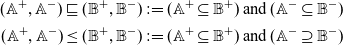 \begin{align*} (\mathbb{A}^+,\mathbb{A}^-) \sqsubseteq (\mathbb{B}^+,\mathbb{B}^-) &:= (\mathbb{A}^+ \subseteq \mathbb{B}^+) \mathbin{\mathrm{and}} (\mathbb{A}^- \subseteq \mathbb{B}^-) \\ (\mathbb{A}^+,\mathbb{A}^-) \leq (\mathbb{B}^+,\mathbb{B}^-) &:= (\mathbb{A}^+ \subseteq \mathbb{B}^+) \mathbin{\mathrm{and}} (\mathbb{A}^- \supseteq \mathbb{B}^-)\end{align*}
The reverse extension order $\mathbb{A} \sqsupseteq \mathbb{B}$
is defined as
$\mathbb{A} \sqsupseteq \mathbb{B}$
is defined as $\mathbb{B} \sqsubseteq \mathbb{A}$
, and supertype order
$\mathbb{B} \sqsubseteq \mathbb{A}$
, and supertype order $\mathbb{A} \geq \mathbb{B}$
is
$\mathbb{A} \geq \mathbb{B}$
is $\mathbb{B} \leq \mathbb{A}$
.
$\mathbb{B} \leq \mathbb{A}$
.
Refinement just expresses basic inclusion: $\mathbb{A}$
refines
$\mathbb{A}$
refines $\mathbb{B}$
when everything in
$\mathbb{B}$
when everything in $\mathbb{A}$
(both term and coterm) is contained within
$\mathbb{A}$
(both term and coterm) is contained within $\mathbb{B}$
. With subtyping, the underlying set orderings go in opposite directions! If
$\mathbb{B}$
. With subtyping, the underlying set orderings go in opposite directions! If $\mathbb{A}$
is a subtype of
$\mathbb{A}$
is a subtype of $\mathbb{B}$
, then
$\mathbb{B}$
, then $\mathbb{A}$
can have fewer terms and more coterms than
$\mathbb{A}$
can have fewer terms and more coterms than $\mathbb{B}$
. While this ordering may seem counter-intuitive, it closely captures the understanding of sound candidates where coterms are tests on terms. If
$\mathbb{B}$
. While this ordering may seem counter-intuitive, it closely captures the understanding of sound candidates where coterms are tests on terms. If $\unicode{x2AEB}$
expresses which terms pass which tests (i.e., coterms), the soundness requires that all of its terms passes each of its tests. If a sound candidate has fewer terms, then it might be able to safely include more tests which were failed by the removed terms. But if a sound candidate has more terms, it might be required to remove some tests that the new terms don’t pass.
$\unicode{x2AEB}$
expresses which terms pass which tests (i.e., coterms), the soundness requires that all of its terms passes each of its tests. If a sound candidate has fewer terms, then it might be able to safely include more tests which were failed by the removed terms. But if a sound candidate has more terms, it might be required to remove some tests that the new terms don’t pass.
This semantics for subtyping formalizes Liskov’s substitution principle (Liskov, 1987): if $\mathbb{A}$
is a subtype of
$\mathbb{A}$
is a subtype of $\mathbb{B}$
, then terms of
$\mathbb{B}$
, then terms of $\mathbb{A}$
are also terms of
$\mathbb{A}$
are also terms of $\mathbb{B}$
because they can be safely used in any context expecting inputs from
$\mathbb{B}$
because they can be safely used in any context expecting inputs from $\mathbb{B}$
(i.e., with any coterm of
$\mathbb{B}$
(i.e., with any coterm of $\mathbb{B}$
). Interestingly, our symmetric model lets us express the logical dual of this substitution principle: if
$\mathbb{B}$
). Interestingly, our symmetric model lets us express the logical dual of this substitution principle: if $\mathbb{A}$
is a subtype of
$\mathbb{A}$
is a subtype of $\mathbb{B}$
, then the coterms of
$\mathbb{B}$
, then the coterms of $\mathbb{B}$
(i.e., contexts expecting inputs of
$\mathbb{B}$
(i.e., contexts expecting inputs of $\mathbb{B}$
) are coterms of
$\mathbb{B}$
) are coterms of $\mathbb{A}$
because they can be safely given any input from
$\mathbb{A}$
because they can be safely given any input from $\mathbb{A}$
. These two principles lead to a natural subtype ordering of reducibility candidates, based on the sets of (co)terms they include.
$\mathbb{A}$
. These two principles lead to a natural subtype ordering of reducibility candidates, based on the sets of (co)terms they include.
The usefulness of this semantic, dual notion of subtyping comes from the way it gives us a complete lattice, which makes it possible to combine and build new candidates from other simpler ones.
>Definition 6.6 (Subtype Lattice). There is a complete lattice of pre-candidates in ${\mathcal{PC}}$
with respect to subtyping order, where the binary intersection (
${\mathcal{PC}}$
with respect to subtyping order, where the binary intersection ( $\mathbb{A} \wedge \mathbb{B}$
, a.k.a meet or greatest lower bound) and union (
$\mathbb{A} \wedge \mathbb{B}$
, a.k.a meet or greatest lower bound) and union ( $\mathbb{A} \vee \mathbb{B}$
, a.k.a join or least upper bound) are defined as:
$\mathbb{A} \vee \mathbb{B}$
, a.k.a join or least upper bound) are defined as:
 \begin{align*} \mathbb{A} \wedge \mathbb{B} &:= (\mathbb{A}^+ \cap \mathbb{B}^+, \mathbb{A}^- \cup \mathbb{B}^-) & \mathbb{A} \vee \mathbb{B} &:= (\mathbb{A}^+ \cup \mathbb{B}^+, \mathbb{A}^- \cap \mathbb{B}^-)\end{align*}
Moreover, these generalize to the intersection ( $\bigwedge \mathcal{A}$
, a.k.a infimum) and union (
$\bigwedge \mathcal{A}$
, a.k.a infimum) and union ( $\bigvee \mathcal{A}$
, a.k.a supremum) of any set
$\bigvee \mathcal{A}$
, a.k.a supremum) of any set $\mathcal{A} \subseteq {\mathcal{PC}}$
of pre-candidates
$\mathcal{A} \subseteq {\mathcal{PC}}$
of pre-candidates
 \begin{align*} \bigwedge \mathcal{A} &:= \left( \bigcap \{\mathbb{A}^+ \mid \mathbb{A} \in \mathcal{A}\} , \bigcup \{\mathbb{A}^- \mid \mathbb{A} \in \mathcal{A}\} \right) \\ \bigvee \mathcal{A} &:= \left( \bigcup \{\mathbb{A}^+ \mid \mathbb{A} \in \mathcal{A}\} , \bigcap \{\mathbb{A}^- \mid \mathbb{A} \in \mathcal{A}\} \right)\end{align*}
The binary least upper bounds and greatest lower bounds have these standard properties:
 \begin{align*} \mathbb{A}\wedge\mathbb{B} &\leq \mathbb{A},\mathbb{B} \leq \mathbb{A}\vee\mathbb{B} & \mathbb{C} \leq \mathbb{A},\mathbb{B} &\implies \mathbb{C} \leq \mathbb{A}\wedge\mathbb{B} & \mathbb{A},\mathbb{B} \leq \mathbb{C} &\implies \mathbb{A}\vee\mathbb{B} \leq \mathbb{C}\end{align*}
In the general case for the bounds on an entire set of pre-candidates, we know:
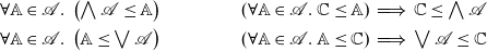 \begin{align*} \forall \mathbb{A} \in \mathcal{A}.~ & \textstyle \left( \bigwedge \mathcal{A} \leq \mathbb{A} \right) & (\forall \mathbb{A} \in \mathcal{A}.~ \mathbb{C} \leq \mathbb{A}) &\implies \textstyle \mathbb{C} \leq \bigwedge \mathcal{A} \\ \forall \mathbb{A} \in \mathcal{A}.~ & \textstyle \left( \mathbb{A} \leq \bigvee \mathcal{A} \right) & (\forall \mathbb{A} \in \mathcal{A}.~ \mathbb{A} \leq \mathbb{C}) &\implies \textstyle \bigvee \mathcal{A} \leq \mathbb{C}\end{align*}
These intersections and unions both preserve soundness, and so they form a lattice of sound candidates in ${\mathcal{SC}}$
as well. However, they do not preserve completeness in general, so they do not form a lattice of reducibility candidates, i.e., sound and complete pre-candidates. Completeness is not preserved because
${\mathcal{SC}}$
as well. However, they do not preserve completeness in general, so they do not form a lattice of reducibility candidates, i.e., sound and complete pre-candidates. Completeness is not preserved because $\mathbb{A} \vee \mathbb{B}$
might be missing some terms (such as
$\mathbb{A} \vee \mathbb{B}$
might be missing some terms (such as $\mu$
s) which could be soundly included, and dually
$\mu$
s) which could be soundly included, and dually $\mathbb{A} \wedge \mathbb{B}$
might be missing some coterms (such as
$\mathbb{A} \wedge \mathbb{B}$
might be missing some coterms (such as ${\tilde{\mu}}$
s). So because all reducibility candidates are sound pre-candidates,
${\tilde{\mu}}$
s). So because all reducibility candidates are sound pre-candidates, $\mathbb{A} \vee \mathbb{B}$
and
$\mathbb{A} \vee \mathbb{B}$
and $\mathbb{A} \wedge \mathbb{B}$
are well-defined, but their results will only be sound candidates (not another reducibility candidate).
Footnote 10
$\mathbb{A} \wedge \mathbb{B}$
are well-defined, but their results will only be sound candidates (not another reducibility candidate).
Footnote 10
What we need is a way to extend arbitrary sound candidates, adding “just enough” to make them full-fledged reducibility candidates. Since there are two possible ways to do this (add the missing terms or add the missing coterms), there are two completions which go in different directions. Also, since the completeness of which (co)terms are guaranteed to be in reducibility candidates is specified up to (co)values, we cannot be sure that absolutely everything ends up in the completed candidate. Instead, we can only ensure that the (co)values that started in the pre-candidate are contained in its completion. This restriction to just the (co)values of a pre-candidate, written $\mathbb{A}^v$
and defined as
$\mathbb{A}^v$
and defined as
 \begin{align*} (\mathbb{A}^+,\mathbb{A}^-)^v &:= (\{V \mid V \in \mathbb{A}^+\}, \{E \mid E \in \mathbb{A}^-\})\end{align*}
becomes a pivotal part of the semantics of types. With this in mind, it follows there are exactly two “ideal” completions, the positive and negative ones, which give a reducibility candidate that is the closest possible to the starting point.
Lemma 6.7 (Positive & Negative Completion). There are two completions, $\operatorname{Pos}$
and
$\operatorname{Pos}$
and $\operatorname{Neg}$
, of any sound candidate
$\operatorname{Neg}$
, of any sound candidate $\mathbb{A}$
with these three properties:
$\mathbb{A}$
with these three properties:
-
1. They are reducibility candidates:
$\operatorname{Pos}(\mathbb{A})$
and
$\operatorname{Neg}(\mathbb{A})$
are both sound and complete. -
2. They are (co)value extensions: Every (co)value of
$\mathbb{A}$
is included in
$\operatorname{Pos}(\mathbb{A})$
and
$\operatorname{Neg}(\mathbb{A})$
.
\begin{align*} \mathbb{A}^v &\sqsubseteq \operatorname{Pos}(\mathbb{A}) & \mathbb{A}^v &\sqsubseteq \operatorname{Neg}(\mathbb{A}) \end{align*}
-
3. They are the least/greatest such candidates: Any reducibility candidate that extends the (co)values of
$\mathbb{A}$
lies between
$\operatorname{Pos}(\mathbb{A})$
and
$\operatorname{Neg}(\mathbb{A})$
, with
$\operatorname{Pos}(\mathbb{A})$
being smaller and
$\operatorname{Neg}(\mathbb{A})$
being greater. In other words, given any reducibility candidate
$\mathbb{C}$
such that
$\mathbb{A}^v \sqsubseteq \mathbb{C}$
:
\begin{align*} \operatorname{Pos}(\mathbb{A}) \leq \mathbb{C} \leq \operatorname{Neg}(\mathbb{A}) \end{align*}


The full proof of these completions (and proofs of the other remaining propositions not given in this section) is given in Appendix 1. We refer to $\operatorname{Pos}(\mathbb{A})$
as the positive completion of
$\operatorname{Pos}(\mathbb{A})$
as the positive completion of $\mathbb{A}$
because it is based entirely on the values of
$\mathbb{A}$
because it is based entirely on the values of $\mathbb{A}$
(i.e., its positive components):
$\mathbb{A}$
(i.e., its positive components): $\operatorname{Pos}(\mathbb{A})$
collects the complete set of coterms that are safe with
$\operatorname{Pos}(\mathbb{A})$
collects the complete set of coterms that are safe with $\mathbb{A}$
’s values and then collects the terms that are safe with the covalues from the previous step, and so on until a fixed point is reached (taking three rounds total). As such, the covalues included in
$\mathbb{A}$
’s values and then collects the terms that are safe with the covalues from the previous step, and so on until a fixed point is reached (taking three rounds total). As such, the covalues included in $\mathbb{A}$
can’t influence the result of
$\mathbb{A}$
can’t influence the result of $\operatorname{Pos}(\mathbb{A})$
. Dually,
$\operatorname{Pos}(\mathbb{A})$
. Dually, $\operatorname{Neg}(\mathbb{A})$
is the negative completion of
$\operatorname{Neg}(\mathbb{A})$
is the negative completion of $\mathbb{A}$
because it is based entirely on
$\mathbb{A}$
because it is based entirely on $\mathbb{A}$
’s covalues in the same manner.
$\mathbb{A}$
’s covalues in the same manner.
Lemma 6.8 (Positive & Negative Invariance). For any sound candidates $\mathbb{A}$
and
$\mathbb{A}$
and $\mathbb{B}$
:
$\mathbb{B}$
:
If the values of
$\mathbb{A}$
and
$\mathbb{B}$
are the same, then
$\operatorname{Pos}(\mathbb{A}) = \operatorname{Pos}(\mathbb{B})$
.If the covalues of
$\mathbb{A}$
and
$\mathbb{B}$
are the same, then
$\operatorname{Neg}(\mathbb{A}) = \operatorname{Neg}(\mathbb{B})$
.


This extra fact gives us another powerful completeness property. We can reason about covalues in the positive candidate $\operatorname{Pos}(\mathbb{A})$
purely in terms of how they interact with
$\operatorname{Pos}(\mathbb{A})$
purely in terms of how they interact with $\mathbb{A}$
’s values, ignoring the rest of
$\mathbb{A}$
’s values, ignoring the rest of $\operatorname{Pos}(\mathbb{A})$
. Dually, we can reason about values in the negative candidate
$\operatorname{Pos}(\mathbb{A})$
. Dually, we can reason about values in the negative candidate $\operatorname{Neg}(\mathbb{A})$
purely based on of
$\operatorname{Neg}(\mathbb{A})$
purely based on of $\mathbb{A}$
’s covalues.
$\mathbb{A}$
’s covalues.
Corollary 6.9 (Strong Positive & Negative Completeness). For any sound candidate $\mathbb{A}$
:
$\mathbb{A}$
:
-
$E \in \operatorname{Pos}(\mathbb{A})$
if and only if
for all
$V \in \mathbb{A}$
.
-
$V \in \operatorname{Neg}(\mathbb{A})$
if and only if
for all
$E \in \mathbb{A}$
.


Proof. Follows directly from Lemmas 6.7 and 6.8.
Now that we know how to turn sound pre-candidates $\mathbb{A}$
into reducibility candidates
$\mathbb{A}$
into reducibility candidates $\operatorname{Pos}(\mathbb{A})$
or
$\operatorname{Pos}(\mathbb{A})$
or $\operatorname{Neg}(\mathbb{A})$
—
$\operatorname{Neg}(\mathbb{A})$
— $\operatorname{Pos}$
and
$\operatorname{Pos}$
and $\operatorname{Neg}$
take anything sound and deliver something sound and complete—we can spell out precisely the subtype-based lattice of reducibility candidates.
$\operatorname{Neg}$
take anything sound and deliver something sound and complete—we can spell out precisely the subtype-based lattice of reducibility candidates.
Theorem 6.10 (Reducibility Subtype Lattice). There is a complete lattice of reducibility candidates in ${\mathcal{RC}}$
with respect to subtyping order, with this binary intersection
${\mathcal{RC}}$
with respect to subtyping order, with this binary intersection $\mathbb{A}\curlywedge\mathbb{B}$
and union
$\mathbb{A}\curlywedge\mathbb{B}$
and union $\mathbb{A}\curlyvee\mathbb{B}$
 \begin{align*} \mathbb{A} \curlywedge \mathbb{B} &:= \operatorname{Neg}(\mathbb{A} \wedge \mathbb{B}) & \mathbb{A} \curlyvee \mathbb{B} &:= \operatorname{Pos}(\mathbb{A} \vee \mathbb{B})\end{align*}
and this intersection (
) and union (
) of any set $\mathcal{A} \subseteq {\mathcal{RC}}$
of reducibility candidates
$\mathcal{A} \subseteq {\mathcal{RC}}$
of reducibility candidates
6.3 Interpretation and adequacy
Using the subtyping lattice, we have enough infrastructure to define an interpretation of types and type-checking judgments as given in Fig. 10. Each type is interpreted as a reducibility candidate. Even though we are dealing with recursive types ( $\operatorname{Nat}$
and
$\operatorname{Nat}$
and $\operatorname{Stream}$
), the candidates for them are defined in a non-recursive way based on Knaster-Tarski’s fixed point construction (Knaster, 1928; Tarski, 1955) and can be read with these intuitions:
$\operatorname{Stream}$
), the candidates for them are defined in a non-recursive way based on Knaster-Tarski’s fixed point construction (Knaster, 1928; Tarski, 1955) and can be read with these intuitions:
-
$[\![ A \to B ]\!]$
is the negatively complete candidate containing all the call stacks built from
$[\![ A ]\!]$
arguments and
$[\![ B ]\!]$
return continuations. Note that this is the same thing (via Lemmas 6.7 and 6.8) as largest candidate containing those call stacks.
-
$[\![ \operatorname{Nat}]\!]$
is the smallest candidate containing
$\operatorname{zero}$
and closed
$\operatorname{succ}$
essor constructors.
-
$[\![ \operatorname{Stream} A ]\!]$
is the largest candidate containing
$\operatorname{head}$
projections expecting an
$[\![ A ]\!]$
element and closed under
$\operatorname{tail}$
projections.


Model of termination and safety of the abstract machine.
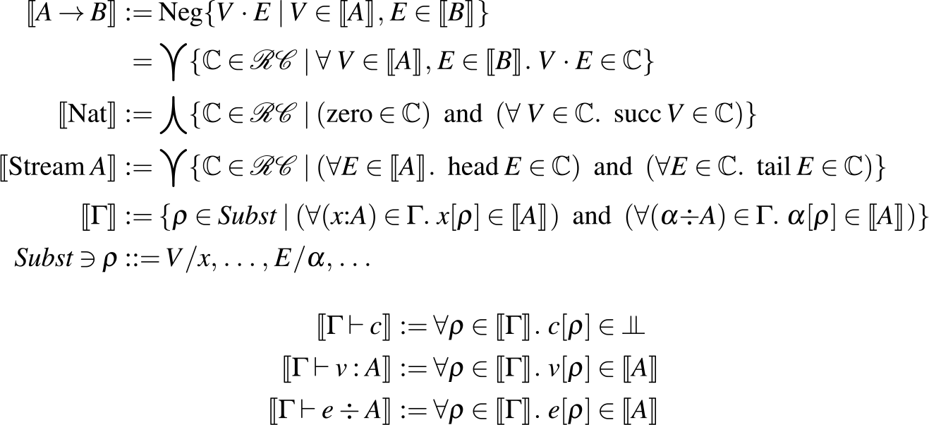
Typing environments ( $\Gamma$
) are interpreted as the set of valid substitutions
$\Gamma$
) are interpreted as the set of valid substitutions $\rho$
which map variables x to values and covariables
$\rho$
which map variables x to values and covariables $\alpha$
to covalues. The interpretation of the typing environment
$\alpha$
to covalues. The interpretation of the typing environment $\Gamma, x : A$
places an additional requirement on these substitutions: a valid substitution
$\Gamma, x : A$
places an additional requirement on these substitutions: a valid substitution $\rho \in [\![\Gamma, x : A]\!]$
must substitute a value of
$\rho \in [\![\Gamma, x : A]\!]$
must substitute a value of $[\![ A ]\!]$
for the variable x, i.e.,
$[\![ A ]\!]$
for the variable x, i.e., $x[{\rho}] \in [\![ A ]\!]$
. Dually, a valid substitution
$x[{\rho}] \in [\![ A ]\!]$
. Dually, a valid substitution $\rho \in [\![\Gamma, \alpha \div A]\!]$
must substitute a covalue of
$\rho \in [\![\Gamma, \alpha \div A]\!]$
must substitute a covalue of $[\![ A ]\!]$
for
$[\![ A ]\!]$
for $\alpha$
, i.e.,
$\alpha$
, i.e., $\alpha[{\rho}] \in [\![ A ]\!]$
. Finally, typing judgments (e.g.,
$\alpha[{\rho}] \in [\![ A ]\!]$
. Finally, typing judgments (e.g., $\Gamma \vdash c \ $
) are interpreted as statements which assert that the command or (co)term belongs to the safe set
$\Gamma \vdash c \ $
) are interpreted as statements which assert that the command or (co)term belongs to the safe set $\unicode{x2AEB}$
or the assigned reducibility candidate for any substitution allowed by the environment. The key lemma is that typing derivations of a judgment ensure that the statement they correspond to holds true.
$\unicode{x2AEB}$
or the assigned reducibility candidate for any substitution allowed by the environment. The key lemma is that typing derivations of a judgment ensure that the statement they correspond to holds true.
Lemma 6.11 (Adequacy).
-
1. If
$\Gamma \vdash c$
is derivable then
$[\![\Gamma \vdash c]\!]$
is true.
-
2. If
$\Gamma \vdash v : A$
is derivable then
$[\![\Gamma \vdash v : A ]\!]$
is true.
-
3. If
$\Gamma \vdash e \div A$
is derivable then
$[\![\Gamma \vdash e \div A ]\!]$
is true.


In order to prove adequacy (Lemma 6.11), we need to know something more about which (co)terms are in the interpretation of types. For example, how do we know that the well-typed call stacks and $\lambda$
-abstractions given by the rules in Fig. 6 end up in
$\lambda$
-abstractions given by the rules in Fig. 6 end up in $[\![ A \to B ]\!]$
? Intuitively, function types themselves are non-recursive. In Fig. 10, the union over the possible candidates
$[\![ A \to B ]\!]$
? Intuitively, function types themselves are non-recursive. In Fig. 10, the union over the possible candidates $\mathbb{C}$
defining
$\mathbb{C}$
defining $[\![ A \to B ]\!]$
requires that certain call stacks must be in each
$[\![ A \to B ]\!]$
requires that certain call stacks must be in each $\mathbb{C}$
, but it does not quantify over the (co)values already in
$\mathbb{C}$
, but it does not quantify over the (co)values already in $\mathbb{C}$
to build upon them. Because of this,
$\mathbb{C}$
to build upon them. Because of this, $[\![ A \to B ]\!]$
is equivalent to the negative candidate
$[\![ A \to B ]\!]$
is equivalent to the negative candidate $\operatorname{Neg}\{V \cdot E \mid V \in [\![ A ]\!], E \in [\![ B ]\!]\}$
, as noted in Fig. 10. It follows from Corollary 6.9 that
$\operatorname{Neg}\{V \cdot E \mid V \in [\![ A ]\!], E \in [\![ B ]\!]\}$
, as noted in Fig. 10. It follows from Corollary 6.9 that $[\![ A \to B ]\!]$
must contain any value which is compatible with just these call stacks, regardless of whatever else might be in
$[\![ A \to B ]\!]$
must contain any value which is compatible with just these call stacks, regardless of whatever else might be in $[\![ A \to B ]\!]$
. This means we can use expansion (Property 6.4) to prove that
$[\![ A \to B ]\!]$
. This means we can use expansion (Property 6.4) to prove that $[\![ A \to B ]\!]$
contains all
$[\![ A \to B ]\!]$
contains all $\lambda$
-abstractions that, when given one of these call stacks, step via
$\lambda$
-abstractions that, when given one of these call stacks, step via $\beta_\to$
reduction to a safe command.
$\beta_\to$
reduction to a safe command.
Lemma 6.12 (Function Abstraction) If $v[{{V}/{x}}] \in [\![ B ]\!]$
for all
$v[{{V}/{x}}] \in [\![ B ]\!]$
for all $V {\in} [\![ A ]\!]$
, then
$V {\in} [\![ A ]\!]$
, then $\lambda x. v \in [\![ A {\to} B ]\!]$
.
$\lambda x. v \in [\![ A {\to} B ]\!]$
.
Proof. Observe that, for any $V \in [\![ A ]\!]$
and
$V \in [\![ A ]\!]$
and $E \in [\![ B ]\!]$
:
$E \in [\![ B ]\!]$
:
 \begin{align*} \langle {\lambda x. v} |\!| {V \cdot E} \rangle &\mapsto \langle {v[{{V}/{x}}]} |\!| {E} \rangle \in \unicode{x2AEB} \end{align*}
where $\langle {v[{{V}/{x}}]} |\!| {E} \rangle \in \unicode{x2AEB}$
is guaranteed due to soundness for the reducibility candidate
$\langle {v[{{V}/{x}}]} |\!| {E} \rangle \in \unicode{x2AEB}$
is guaranteed due to soundness for the reducibility candidate $[\![ B ]\!]$
. By expansion (Property 6.4), we know that
$[\![ B ]\!]$
. By expansion (Property 6.4), we know that $\langle {\lambda x. v} |\!| {V \cdot E} \rangle \in \unicode{x2AEB}$
as well. So from Corollary 6.9:
$\langle {\lambda x. v} |\!| {V \cdot E} \rangle \in \unicode{x2AEB}$
as well. So from Corollary 6.9:
 \begin{equation*} \lambda x. v \in \operatorname{Neg}\{V \cdot E \mid V \in [\![ A ]\!], E \in [\![ B ]\!]\} = [\![ A \to B ]\!] \end{equation*}
But what about $[\![ \operatorname{Nat}]\!]$
and
$[\![ \operatorname{Nat}]\!]$
and $[\![ \operatorname{Stream} A ]\!]$
? The interpretations of (co)inductive types are not exactly instances of
$[\![ \operatorname{Stream} A ]\!]$
? The interpretations of (co)inductive types are not exactly instances of $\operatorname{Pos}$
or
$\operatorname{Pos}$
or $\operatorname{Neg}$
as written, because unlike
$\operatorname{Neg}$
as written, because unlike $[\![ A \to B ]\!]$
, they quantify over elements in the possible
$[\![ A \to B ]\!]$
, they quantify over elements in the possible $\mathbb{C}$
s they are made from. This lets us say these
$\mathbb{C}$
s they are made from. This lets us say these $\mathbb{C}$
s are closed under
$\mathbb{C}$
s are closed under $\operatorname{succ}$
or
$\operatorname{succ}$
or $\operatorname{tail}$
, but it means that we cannot identify a priori a set of (co)values that generate the candidate independent of each
$\operatorname{tail}$
, but it means that we cannot identify a priori a set of (co)values that generate the candidate independent of each $\mathbb{C}$
.
$\mathbb{C}$
.
A solution to this conundrum is to instead describe these (co)inductive types incrementally, building them step-by-step instead of all-at once à la Kleene’s fixed point construction (Kleene, 1952). For example, the set of the natural numbers can be defined incrementally from a series of finite approximations by beginning with the empty set, and then at each step adding the number 0 and the successor of the previous set:
 \begin{align*} \mathbb{N}_0 &:= \{\} & \mathbb{N}_{i+1} &:= \{0\} \cup \{n+1 \mid n \in \mathbb{N}_i\} & \mathbb{N} &:= \bigcup_{i=0}^\infty \{\mathbb{N}_i\}\end{align*}
So that each $\mathbb{N}_i$
contains only the numbers less than i. The final set of all natural numbers,
$\mathbb{N}_i$
contains only the numbers less than i. The final set of all natural numbers, $\mathbb{N}$
, is then the union of each approximation
$\mathbb{N}$
, is then the union of each approximation $\mathbb{N}_i$
along the way. Likewise, we can do a similar incremental definition of finite approximations of
$\mathbb{N}_i$
along the way. Likewise, we can do a similar incremental definition of finite approximations of $[\![ \operatorname{Nat}]\!]$
like so:
$[\![ \operatorname{Nat}]\!]$
like so:

The starting approximation $[\![ \operatorname{Nat}]\!]_0$
is the smallest reducibility candidate, which is given by
$[\![ \operatorname{Nat}]\!]_0$
is the smallest reducibility candidate, which is given by $\operatorname{Pos}\{\}$
. From there, the next approximations are given by the positive candidate containing at least
$\operatorname{Pos}\{\}$
. From there, the next approximations are given by the positive candidate containing at least $\operatorname{zero}$
and the
$\operatorname{zero}$
and the $\operatorname{successor}$
of every value of their predecessor. This construction mimics the approximations
$\operatorname{successor}$
of every value of their predecessor. This construction mimics the approximations $\mathbb{N}_i$
, where we start with the smallest possible base and incrementally build larger and larger reducibility candidates that more accurately approximate the limit.
$\mathbb{N}_i$
, where we start with the smallest possible base and incrementally build larger and larger reducibility candidates that more accurately approximate the limit.
The typical incremental coinductive definition is usually presented in the reverse direction: start out with the “biggest” set (whatever that is), and trim it down step-by-step. Instead, the coinductive construction of reducibility candidates is much more concrete, since they form a complete lattice (with respect to subtyping). There is a specific biggest candidate
(equal to
) containing every term possible and the fewest coterms allowed. From there, we can add explicitly more coterms to each successive approximation, which shrinks the candidate by ruling out some terms that do not run safely with them. Thus, the incremental approximations of $[\![ \operatorname{Stream} A ]\!]$
are defined negatively as:
$[\![ \operatorname{Stream} A ]\!]$
are defined negatively as:

We start with the biggest possible candidate given by $\operatorname{Neg}\{\}$
. From there, the next approximations are given by the negative candidate containing at least
$\operatorname{Neg}\{\}$
. From there, the next approximations are given by the negative candidate containing at least $\operatorname{head} E$
(for any E expecting an element of type
$\operatorname{head} E$
(for any E expecting an element of type $[\![ A ]\!]$
) and the
$[\![ A ]\!]$
) and the $\operatorname{tail}$
of every covalue in the previous approximation. The net effect is that
$\operatorname{tail}$
of every covalue in the previous approximation. The net effect is that $[\![ \operatorname{Stream} A ]\!]_i$
definitely contains all continuations built from (at most) i
$[\![ \operatorname{Stream} A ]\!]_i$
definitely contains all continuations built from (at most) i $\operatorname{head}$
and
$\operatorname{head}$
and $\operatorname{tail}$
destructors. As with
$\operatorname{tail}$
destructors. As with $[\![ \operatorname{Nat} ]\!]_i$
, the goal is to show that
$[\![ \operatorname{Nat} ]\!]_i$
, the goal is to show that $[\![ \operatorname{Stream} A ]\!]$
is the limit of
$[\![ \operatorname{Stream} A ]\!]$
is the limit of $[\![ \operatorname{Stream} A ]\!]_i$
, i.e., that it is the intersection of all finite approximations.
$[\![ \operatorname{Stream} A ]\!]_i$
, i.e., that it is the intersection of all finite approximations.
Lemma 6.13 ((Co)Induction Inversion).

This fact makes it possible to use expansion (Property 6.4) and strong completeness (Corollary 6.9) to prove that the recursor belongs to each of the approximations $[\![ \operatorname{Nat}]\!]_i$
; and thus also to
$[\![ \operatorname{Nat}]\!]_i$
; and thus also to
![]() by induction on i. Dually, the corecursor belongs to each approximation
by induction on i. Dually, the corecursor belongs to each approximation $[\![ \operatorname{Stream} A ]\!]_i$
, so it is included in
$[\![ \operatorname{Stream} A ]\!]_i$
, so it is included in
![]() . This proof of safety for (co)recursion is the final step in proving overall adequacy (Lemma 6.11). In turn, the ultimate type safety and termination property we are after is a special case of a more general notion of observable safety and termination, which follows directly from adequacy for certain typing environments.
. This proof of safety for (co)recursion is the final step in proving overall adequacy (Lemma 6.11). In turn, the ultimate type safety and termination property we are after is a special case of a more general notion of observable safety and termination, which follows directly from adequacy for certain typing environments.
Theorem 6.14 (Type safety & Termination of Programs). If $\alpha\div\operatorname{Nat} \vdash c \ $
in the (co)recursive abstract machine then
$\alpha\div\operatorname{Nat} \vdash c \ $
in the (co)recursive abstract machine then $c \mathrel{\mapsto\!\!\!\!\to} \langle {\operatorname{zero}} |\!| {\alpha} \rangle$
or
$c \mathrel{\mapsto\!\!\!\!\to} \langle {\operatorname{zero}} |\!| {\alpha} \rangle$
or $c \mathrel{\mapsto\!\!\!\!\to} \langle {\operatorname{succ} V} |\!| {\alpha} \rangle$
for some V.
$c \mathrel{\mapsto\!\!\!\!\to} \langle {\operatorname{succ} V} |\!| {\alpha} \rangle$
for some V.
Proof. From Lemma 6.11, we have $[\![\alpha\div\operatorname{Nat} \vdash c \ ]\!]$
. That is, for all
$[\![\alpha\div\operatorname{Nat} \vdash c \ ]\!]$
. That is, for all $E \in [\![ \operatorname{Nat} ]\!]$
,
$E \in [\![ \operatorname{Nat} ]\!]$
, $c[{{E}/{\alpha}}] \in \unicode{x2AEB}$
. Note that both
$c[{{E}/{\alpha}}] \in \unicode{x2AEB}$
. Note that both $\langle {\operatorname{zero}} |\!| {\alpha} \rangle \in \unicode{x2AEB}$
and
$\langle {\operatorname{zero}} |\!| {\alpha} \rangle \in \unicode{x2AEB}$
and $\langle {\operatorname{succ} V} |\!| {\alpha} \rangle \in \unicode{x2AEB}$
(for any V whatsoever) by definition of
$\langle {\operatorname{succ} V} |\!| {\alpha} \rangle \in \unicode{x2AEB}$
(for any V whatsoever) by definition of $\unicode{x2AEB}$
(Definition 6.1). So by Corollary 6.9,
$\unicode{x2AEB}$
(Definition 6.1). So by Corollary 6.9, $\alpha$
itself is a member of
$\alpha$
itself is a member of $[\![ \operatorname{Nat} ]\!]$
, i.e.,
$[\![ \operatorname{Nat} ]\!]$
, i.e., $\alpha \in [\![ \operatorname{Nat} ]\!]$
. Thus,
$\alpha \in [\![ \operatorname{Nat} ]\!]$
. Thus, $c[{{\alpha}/{\alpha}}] = c \in \unicode{x2AEB}$
, and the necessary reduction follows from the definition of
$c[{{\alpha}/{\alpha}}] = c \in \unicode{x2AEB}$
, and the necessary reduction follows from the definition of $\unicode{x2AEB}$
.
$\unicode{x2AEB}$
.
Intermezzo 6.15. The wordings of Theorems 3.2 and 6.14 are meant to reflect the typical statement of type safety for functional and $\lambda$
-calculus-based languages. In a
$\lambda$
-calculus-based languages. In a $\lambda$
-based language, type safety (and notably the “progress” half of a progress and preservation proof) is limited to closed programs which return some basic, observable data type like a boolean value, string, number, or list. For example, type safety might ensure that a term M never gets stuck when
$\lambda$
-based language, type safety (and notably the “progress” half of a progress and preservation proof) is limited to closed programs which return some basic, observable data type like a boolean value, string, number, or list. For example, type safety might ensure that a term M never gets stuck when $\bullet \vdash M : \operatorname{Nat}$
. In our typed abstract machine, commands are the unit of execution rather than terms. So instead of a closed term
$\bullet \vdash M : \operatorname{Nat}$
. In our typed abstract machine, commands are the unit of execution rather than terms. So instead of a closed term $\bullet \vdash v : \operatorname{Nat}$
, we state type safety and termination for a starting command like
$\bullet \vdash v : \operatorname{Nat}$
, we state type safety and termination for a starting command like $\alpha \div \operatorname{Nat} \vdash \langle {v} |\!| {\alpha} \rangle \ $
, where v is the closed “source program” and
$\alpha \div \operatorname{Nat} \vdash \langle {v} |\!| {\alpha} \rangle \ $
, where v is the closed “source program” and $\alpha$
represents an initial continuation or empty context waiting for the final result, which is expected to be a natural number.
$\alpha$
represents an initial continuation or empty context waiting for the final result, which is expected to be a natural number.
The fact that the safe command described by Theorems 3.2 and 6.14 is not closed, Footnote 11 but has a free covariable, raises the question: can safety and termination be generalized to cover other open commands with additional variables or covariables? And what might we require of those open commands in general to still ensure termination?
It turns out, very little of the proof methodology depends the specifics of our particular notion of safety captured by the sets of commands $\unicode{x2AEB}$
and
$\unicode{x2AEB}$
and $\mathit{Final}$
from Definition 6.1. Rather, the only property of these sets that is pervasively used is the Property 6.4 that
$\mathit{Final}$
from Definition 6.1. Rather, the only property of these sets that is pervasively used is the Property 6.4 that $\unicode{x2AEB}$
is closed under expansion (
$\unicode{x2AEB}$
is closed under expansion ( $c \mapsto c' \in \unicode{x2AEB}$
implies
$c \mapsto c' \in \unicode{x2AEB}$
implies $c \in \unicode{x2AEB}$
). In fact, there is only one place in the proof that requires another fact about
$c \in \unicode{x2AEB}$
). In fact, there is only one place in the proof that requires another fact about $\unicode{x2AEB}$
, which is showing that
$\unicode{x2AEB}$
, which is showing that
![]() for Lemma 6.13; this step uses the fact that there is at least one command, namely
for Lemma 6.13; this step uses the fact that there is at least one command, namely $\langle {\operatorname{zero}} |\!| {\alpha} \rangle$
, in
$\langle {\operatorname{zero}} |\!| {\alpha} \rangle$
, in $\unicode{x2AEB}$
. However, this choice of example inhabitant of
$\unicode{x2AEB}$
. However, this choice of example inhabitant of $\unicode{x2AEB}$
is arbitrary, and could be replaced with any other choice of
$\unicode{x2AEB}$
is arbitrary, and could be replaced with any other choice of $\langle {V_0} |\!| {E_0} \rangle \in \unicode{x2AEB}$
without otherwise changing the proof.
$\langle {V_0} |\!| {E_0} \rangle \in \unicode{x2AEB}$
without otherwise changing the proof.
This independence of the general proof methodology from the notion of safety (captured by $\unicode{x2AEB}$
) makes it a rather straightforward exercise to generalize to other results by just redefining the set
$\unicode{x2AEB}$
) makes it a rather straightforward exercise to generalize to other results by just redefining the set $\unicode{x2AEB}$
of safe commands. For example, we could consider additional examples of
$\unicode{x2AEB}$
of safe commands. For example, we could consider additional examples of $\mathit{Final}$
commands which also includes stopping with any variable x observed by a destructor
$\mathit{Final}$
commands which also includes stopping with any variable x observed by a destructor $\operatorname{head} E$
,
$\operatorname{head} E$
, $\operatorname{tail} E$
, or
$\operatorname{tail} E$
, or $V \cdot E$
, letting us observe a larger collection of safe commands
$V \cdot E$
, letting us observe a larger collection of safe commands $\unicode{x2AEB}$
.
$\unicode{x2AEB}$
.
Definition 6.16 (Observable Safety). The set of observably safe commands, $\unicode{x2AEB}$
, is:
$\unicode{x2AEB}$
, is:

The same theorems still hold, up to and including adequacy (Lemma 6.11) and the specific lemmas about the nature of function and (co)inductive types (Lemmas 6.12 and 6.13) after replacing Definition 6.1 with Definition 6.16. As a consequence, we can use this bigger definition of $\unicode{x2AEB}$
to meaningfully observe a larger collection of safe commands than before.
$\unicode{x2AEB}$
to meaningfully observe a larger collection of safe commands than before.
Definition 6.17 (Observable Typing Environment). A typing environment $\Gamma$
is observable when every covariable in
$\Gamma$
is observable when every covariable in $\Gamma$
has the type
$\Gamma$
has the type $\operatorname{Nat}$
, and every variable in
$\operatorname{Nat}$
, and every variable in $\Gamma$
has the type
$\Gamma$
has the type $A \to B$
or
$A \to B$
or $\operatorname{Stream} A$
for some type(s) A and B.
$\operatorname{Stream} A$
for some type(s) A and B.
Theorem 6.18 (Observable Safety & Termination). Given any observable typing environment $\Gamma$
, if
$\Gamma$
, if $\Gamma \vdash c \ $
in the (co)recursive abstract machine then
$\Gamma \vdash c \ $
in the (co)recursive abstract machine then $c \mathrel{\mapsto\!\!\!\!\to} c' \in \mathit{Final}$
, as per Definition 6.16.
$c \mathrel{\mapsto\!\!\!\!\to} c' \in \mathit{Final}$
, as per Definition 6.16.
Proof First, note that the interpretations of specific types are guaranteed to contain variables or covariables as follows:
-
1.
$\alpha \in [\![ \operatorname{Nat} ]\!]$
. This is because
$\langle {\operatorname{zero}} |\!| {\alpha} \rangle \in \mathit{Final} \supseteq \unicode{x2AEB}$
and
for any V whatsoever by definition of
$\unicode{x2AEB}$
(Definition 6.16).So by the updated Corollary 6.9,
$\alpha$
itself is a member of
$[\![ \operatorname{Nat} ]\!]$
. -
2.
$x \in [\![ \operatorname{Stream} A ]\!]$
. This is because
$\langle {x} |\!| {\operatorname{head} E} \rangle \in \mathit{Final} \supseteq \unicode{x2AEB}$
and
$\langle {x} |\!| {\operatorname{tail} E} \rangle \in \mathit{Final} \supseteq \unicode{x2AEB}$
for any E by definition of
$\unicode{x2AEB}$
(Definition 6.16), so x is a member of
$[\![ \operatorname{Stream} A ]\!]$
for any A by the updated Corollary 6.9. -
3.
$x \in [\![ A \to B ]\!]$
. This is because
$\langle {x} |\!| {V \cdot E} \rangle \in \mathit{Final} \supseteq \unicode{x2AEB}$
for any V and E by definition of
$\unicode{x2AEB}$
(Definition 6.16), so x is a member of
$[\![ A \to B ]\!]$
for any A and B by the updated Corollary 6.9.


It follows that for any observable typing environment $\Gamma$
, there is
$\Gamma$
, there is $\mathit{id}_\Gamma \in [\![ \Gamma ]\!]$
where the identity substitution
$\mathit{id}_\Gamma \in [\![ \Gamma ]\!]$
where the identity substitution $\mathit{id}_\Gamma$
is defined as:
$\mathit{id}_\Gamma$
is defined as:
 \begin{align*} \mathit{id}_\Gamma(x) &= x &(\text{if } (x : A) &\in \Gamma) & \mathit{id}_\Gamma(\alpha) &= \alpha &(\text{if } (\alpha \div A) &\in \Gamma) \end{align*}
Now, updated adequacy (Lemma 6.11) ensures $[\![\Gamma \vdash c \ ]\!]$
. That is, for all
$[\![\Gamma \vdash c \ ]\!]$
. That is, for all $\rho \in [\![ \Gamma ]\!]$
,
$\rho \in [\![ \Gamma ]\!]$
, $c[{\rho}] \in \unicode{x2AEB}$
. Since
$c[{\rho}] \in \unicode{x2AEB}$
. Since $\Gamma$
is observable,
$\Gamma$
is observable, $\mathit{id}_\Gamma \in [\![ \Gamma ]\!]$
, and thus
$\mathit{id}_\Gamma \in [\![ \Gamma ]\!]$
, and thus $c[{\mathit{id}_\Gamma}] = c \in \unicode{x2AEB}$
. So by definition of
$c[{\mathit{id}_\Gamma}] = c \in \unicode{x2AEB}$
. So by definition of $\unicode{x2AEB}$
(Definition 6.16),
$\unicode{x2AEB}$
(Definition 6.16), $c \mathrel{\mapsto\!\!\!\!\to} c' \in \mathit{Final}$
.
$c \mathrel{\mapsto\!\!\!\!\to} c' \in \mathit{Final}$
.
7 Related work
The corecursor presented here is a computational interpretation of the categorical model of corecursion in a coalgebra. A coalgebra for a functor F is defined by a morphism $\alpha : A \to F(A)$
, and it is (strongly) terminal if there always exists a unique morphism from any other coalgebra of F into it, satisfying the usual commutation properties (i.e., the coalgebra given by
$\alpha : A \to F(A)$
, and it is (strongly) terminal if there always exists a unique morphism from any other coalgebra of F into it, satisfying the usual commutation properties (i.e., the coalgebra given by $\alpha : A \to F(A)$
is the terminal object in the category of F-coalgebras). As a way to characterize the difference between coiteration and corecursion, Geuvers (1992) relaxes this usual requirement to weakly terminal coalgebras, for which there might be several non-unique morphisms with the correct properties into the weakly terminal coalgebra. A corecursive coalgebra extends this idea by ensuring commutation with other morphisms of the form
$\alpha : A \to F(A)$
is the terminal object in the category of F-coalgebras). As a way to characterize the difference between coiteration and corecursion, Geuvers (1992) relaxes this usual requirement to weakly terminal coalgebras, for which there might be several non-unique morphisms with the correct properties into the weakly terminal coalgebra. A corecursive coalgebra extends this idea by ensuring commutation with other morphisms of the form $X \to F(A + X)$
, rather than just another F-coalgebra
$X \to F(A + X)$
, rather than just another F-coalgebra $X \to F(X)$
.
$X \to F(X)$
.
The dual notion to Geuvers (1992)’s corecursive F-coalgebra is (therein) called a recursive F-algebra: an algebra $\alpha : F(A) \to A$
that is only weakly initial—there is always a morphism from
$\alpha : F(A) \to A$
that is only weakly initial—there is always a morphism from $\alpha$
to any other F-algebra, but it need not be unique—such that it commutes with every morphism of the form
$\alpha$
to any other F-algebra, but it need not be unique—such that it commutes with every morphism of the form $F(A \times X) \to X$
, not just F-algebras
$F(A \times X) \to X$
, not just F-algebras $F(X) \to X$
. Computationally speaking, the generalization to
$F(X) \to X$
. Computationally speaking, the generalization to $F(A \times X) \to X$
corresponds to the difference between the System T recursor and iterator: the
$F(A \times X) \to X$
corresponds to the difference between the System T recursor and iterator: the $A \times X$
corresponds to the two inputs in the successor case of the recursor (with A being the immediate predecessor and X being the solution on the predecessor), in comparison to the single input for the successor case of the iterator (who is only given the solution on the predecessor, but not the predecessor itself). Analogously, the
$A \times X$
corresponds to the two inputs in the successor case of the recursor (with A being the immediate predecessor and X being the solution on the predecessor), in comparison to the single input for the successor case of the iterator (who is only given the solution on the predecessor, but not the predecessor itself). Analogously, the $A + X$
in the commutation with
$A + X$
in the commutation with $X \to F(A + X)$
for a corecursive coalgebra is interpreted as an (intuitionistic) sum type in the pure (i.e., side-effect free)
$X \to F(A + X)$
for a corecursive coalgebra is interpreted as an (intuitionistic) sum type in the pure (i.e., side-effect free) $\lambda$
-calculus model by Geuvers (1992):
$\lambda$
-calculus model by Geuvers (1992): $X + A$
stands for the ordinary data type with two constructors for injecting either of X or A into the sum. Here, we use an interpretation of
$X + A$
stands for the ordinary data type with two constructors for injecting either of X or A into the sum. Here, we use an interpretation of $A + X$
as expressing the classical disjunction of multiple conclusions, represented in the calculus by multiple continuations passed simultaneously to one term. The multi-continuation interpretation of a classical disjunction gives improved generality, and can express some corecursive algorithms that the intuitionistic interpretation cannot (Downen & Ariola, 2021).
$A + X$
as expressing the classical disjunction of multiple conclusions, represented in the calculus by multiple continuations passed simultaneously to one term. The multi-continuation interpretation of a classical disjunction gives improved generality, and can express some corecursive algorithms that the intuitionistic interpretation cannot (Downen & Ariola, 2021).
The coiterator, which we define as the restriction of the corecursor to never short-cut corecursion, corresponds exactly to the Harper’s strgen (Harper, 2016). In this sense, the corecursor is a conservative extension of the purely functional coiterator. Coiteration with control operators is considered in Barthe & Uustalu (2002), which gives a call-by-name CPS translation for a stream coiterator and constructor, corresponding to $\operatorname{\mathbf{coiter}}$
and
$\operatorname{\mathbf{coiter}}$
and $\operatorname{\mathbf{cocase}}$
, but not for
$\operatorname{\mathbf{cocase}}$
, but not for $\operatorname{\mathbf{corec}}$
. Here, the use of an abstract machine serves a similar role as CPS—making explicit information and control flow—but allows us to use the same translation for both call-by-value and call-by-name. An alternative approach to (co)recursive combinators is sized types (Hughes et al., 1996; Abel, 2006), which give the programmer control over recursion while still ensuring termination, and have been used for both purely functional (Abel & Pientka, 2013) and classical (Downen et al., Reference Downen, Johnson-Freyd and Ariola2015) coinductive types. Both of these approaches express (co)recursive algorithms directly in terms of (co)pattern matching.
$\operatorname{\mathbf{corec}}$
. Here, the use of an abstract machine serves a similar role as CPS—making explicit information and control flow—but allows us to use the same translation for both call-by-value and call-by-name. An alternative approach to (co)recursive combinators is sized types (Hughes et al., 1996; Abel, 2006), which give the programmer control over recursion while still ensuring termination, and have been used for both purely functional (Abel & Pientka, 2013) and classical (Downen et al., Reference Downen, Johnson-Freyd and Ariola2015) coinductive types. Both of these approaches express (co)recursive algorithms directly in terms of (co)pattern matching.
In the context of more practical programming, Charity (Fukushima & Cockett, 1992) is a total functional programming language whose design is based closely on categorical semantics, which can express the duality between inductive and coinductive types. As such, it included primitives for iteration and coiteration, as well as case and cocase, similar to $\operatorname{\mathbf{coiter}}$
and
$\operatorname{\mathbf{coiter}}$
and $\operatorname{\mathbf{cocase}}$
primitives in the calculus shown here. More recently, the OCaml language has been extended with copatterns (Regis-Gianas & Laforgue, 2017) as well as an explicit corec form Jeannin et al. (2017) to allow for corecursive functional programming. In other programming paradigms, applications of corecursion have been studied in the context of object-oriented programming (Ancona & Zucca, 2013, 2012a,b)—with a focus on modeling finite structures with cycles via regular corecursion—and logic programming (Ancona, 2013; Dagnino et al., 2020; Dagnino, 2020) with non-well-founded structures in terms of coaxioms that are applied at “infinite” depth in an proof tree.
$\operatorname{\mathbf{cocase}}$
primitives in the calculus shown here. More recently, the OCaml language has been extended with copatterns (Regis-Gianas & Laforgue, 2017) as well as an explicit corec form Jeannin et al. (2017) to allow for corecursive functional programming. In other programming paradigms, applications of corecursion have been studied in the context of object-oriented programming (Ancona & Zucca, 2013, 2012a,b)—with a focus on modeling finite structures with cycles via regular corecursion—and logic programming (Ancona, 2013; Dagnino et al., 2020; Dagnino, 2020) with non-well-founded structures in terms of coaxioms that are applied at “infinite” depth in an proof tree.
Our investigation on evaluation strategy showed the (dual) impact of call-by-value versus call-by-name evaluation (Curien & Herbelin, 2000; Wadler, Reference Wadler2003) on the efficiency of (co)recursion. In contrast to having a monolithic evaluation strategy, another approach is to use a hybrid evaluation strategy as done by call-by-push-value (Levy, 2001) or polarized languages (Zeilberger, 2009; Munch-Maccagnoni, 2013). With a hybrid approach, we could define one language which has the efficient version of both the recursor and corecursor. Polarity also allows for incorporating other evaluation strategies, such as call-by-need which shares the work of computations (Downen & Ariola, 2018a; McDermott & Mycroft, 2019). We leave the investigation of a polarized version of corecursion to future work.
8 Conclusion
This paper provides a foundational calculus for (co)recursion in programs phrased in terms of an abstract machine language. The impact of evaluation strategy is also illustrated, where call-by-value and call-by-name have (opposite) advantages for the efficiency of corecursion and recursion, respectively. These (co)recursion schemes are captured by (co)data types whose duality is made apparent by the language of the abstract machine. In particular, inductive data types, like numbers, revolve around constructing concrete, finite values, so that observations on numbers may be abstract and unbounded. Dually, coinductive codata types, like streams, revolve around concrete, finite observations, so that values may be abstract and unbounded objects. The computational interpretation of this duality lets us bring out hidden connections underlying the implementation of recursion and corecursion. For example, the explicit “seed” or accumulator usually used to generate infinite streams is, in fact, dual to the implicitly growing evaluation context of recursive calls. To show that the combination of primitive recursion and corecursion is well-behaved—that is, every program safely terminates with an answer—we interpreted the type system as a form of classical (bi)orthogonality model capable of handling first-class control effects, and extended with (co)inductive reducibility candidates. Our model reveals how the incremental Kleene-style and wholesale Knaster-Tarski-style constructions of greatest and least fixed points have different advantages for reasoning about program behavior. By showing the two fixed point constructions are the same—a non-trivial task for types of effectful computation—we get a complete picture of the mechanics of classical (co)recursion.
Acknowledgments
We would like to thank the anonymous reviewers for their helpful suggestions and feedback for improving the presentation of this article. This work is supported by the National Science Foundation under Grant No. 1719158.
Conflicts of interest
None.
1 Proof of type safety and termination
Here we give the full details to the proof of the main result, Theorem 6.14, ensuring both safety and termination for all well-typed, executable commands. We use a proof technique suitable for abstract machines based on (Downen et al., Reference Downen, Johnson-Freyd and Ariola2020, Reference Downen, Ariola and Ghilezan2019), which we extend with the inductive type $\operatorname{Nat}$
and the coinductive type
$\operatorname{Nat}$
and the coinductive type $\operatorname{Stream} A$
. To begin in Appendices 1.1 to 1.3, we give a self-contained introduction and summary of the fundamental concepts and results from Downen et al. (Reference Downen, Johnson-Freyd and Ariola2020, Reference Downen, Ariola and Ghilezan2019). Appendix 1.2 in particular gives a new account of positive and negative completion which simplifies the sections that follow. From there, Appendix 1.4 establishes the definition and properties of the (co)inductive types
$\operatorname{Stream} A$
. To begin in Appendices 1.1 to 1.3, we give a self-contained introduction and summary of the fundamental concepts and results from Downen et al. (Reference Downen, Johnson-Freyd and Ariola2020, Reference Downen, Ariola and Ghilezan2019). Appendix 1.2 in particular gives a new account of positive and negative completion which simplifies the sections that follow. From there, Appendix 1.4 establishes the definition and properties of the (co)inductive types $\operatorname{Nat}$
and
$\operatorname{Nat}$
and $\operatorname{Stream} A$
in this model, which lets us prove the fundamental adequacy lemma in Appendix 1.5.
$\operatorname{Stream} A$
in this model, which lets us prove the fundamental adequacy lemma in Appendix 1.5.
1.1 Orthogonal fixed point candidates
Our proof technique revolves around pre-candidates (Definition 6.2) and their more informative siblings reducibility candidates. The first, and most important, operation on pre-candidates is orthogonality. Intuitively, on the one side orthogonality identifies all the terms that are safe with everything in a given set of coterms, and on the other side, it identifies the coterms that are safe with a set of terms. These two dual operations converting back and forth between terms and coterms naturally extend to a single operation on pre-candidates.
Definition 1.1 (Orthogonality). The orthogonal of any set of terms, $\mathbb{A}^+$
, written
$\mathbb{A}^+$
, written $\mathbb{A}^{+\unicode{x2AEB}}$
, is the set of coterms that form safe commands (i.e., in
$\mathbb{A}^{+\unicode{x2AEB}}$
, is the set of coterms that form safe commands (i.e., in $\unicode{x2AEB}$
) with all of
$\unicode{x2AEB}$
) with all of $\mathbb{A}^+$
:
$\mathbb{A}^+$
:
 \begin{align*} \mathbb{A}^{+\unicode{x2AEB}} &:= \{ e \mid \forall v \in \mathbb{A}^+.~ \langle {v} |\!| {e} \rangle \in \unicode{x2AEB} \}\end{align*}
Dually, the orthogonal of any set of coterms $\mathbb{A}^-$
, also written
$\mathbb{A}^-$
, also written $\mathbb{A}^{-\unicode{x2AEB}}$
and disambiguated by context, is the set of terms that form safe commands with all of
$\mathbb{A}^{-\unicode{x2AEB}}$
and disambiguated by context, is the set of terms that form safe commands with all of $\mathbb{A}^-$
:
$\mathbb{A}^-$
:
 \begin{align*} \mathbb{A}^{-\unicode{x2AEB}} &:= \{ v \mid \forall e \in \mathbb{A}^-.~ \langle {v} |\!| {e} \rangle \in \unicode{x2AEB} \}\end{align*}
Finally, the orthogonal of any pre-candidate $\mathbb{A} = (\mathbb{A}^+, \mathbb{A}^-)$
is:
$\mathbb{A} = (\mathbb{A}^+, \mathbb{A}^-)$
is:
 \begin{align*} (\mathbb{A}^+, \mathbb{A}^-)^\unicode{x2AEB} &:= (\mathbb{A}^{-\unicode{x2AEB}}, \mathbb{A}^{+\unicode{x2AEB}})\end{align*}
As a shorthand for mapping over sets, given any set of pre-candidates $\mathcal{A} \subseteq {\mathcal{PC}}$
, we write
$\mathcal{A} \subseteq {\mathcal{PC}}$
, we write $\mathcal{A}^{\unicode{x2AEB}*}$
for the set of orthogonals to each pre-candidate in
$\mathcal{A}^{\unicode{x2AEB}*}$
for the set of orthogonals to each pre-candidate in $\mathcal{A}$
:
$\mathcal{A}$
:
 \begin{align*} \mathcal{A}^{\unicode{x2AEB}*} &:= \{\mathbb{A}^\unicode{x2AEB} \mid \mathbb{A}^\unicode{x2AEB} \in \mathcal{A}\}\end{align*}
We use the same notation for the orthogonals of any set of term-sets ( $\mathcal{A} \subseteq \wp(\mathit{Term})$
) or coterm-sets (
$\mathcal{A} \subseteq \wp(\mathit{Term})$
) or coterm-sets ( $\mathcal{A} \subseteq \wp(\mathit{CoTerm})$
), individually.
$\mathcal{A} \subseteq \wp(\mathit{CoTerm})$
), individually.
Orthogonality is interesting primarily because of the logical structure it creates among pre-candidates. In particular, orthogonality behaves very much like intuitionistic negation ( $\neg$
). Intuitionistic logic rejects double negation elimination (
$\neg$
). Intuitionistic logic rejects double negation elimination ( $\neg \neg A \iff A$
) in favor of the weaker principle of double negation introduction (
$\neg \neg A \iff A$
) in favor of the weaker principle of double negation introduction ( $A \implies \neg \neg A$
). This fundamental property of intuitionistic negation is mimicked by pre-candidate orthogonality.
$A \implies \neg \neg A$
). This fundamental property of intuitionistic negation is mimicked by pre-candidate orthogonality.
Property 1.2 (Orthogonal Negation). The following holds for any pre-candidates $\mathbb{A}$
and
$\mathbb{A}$
and $\mathbb{B}$
:
$\mathbb{B}$
:
-
1. Contrapositive (i.e., antitonicity):
$\mathbb{A} \sqsubseteq \mathbb{B}$
implies
$\mathbb{B}^{\unicode{x2AEB}} \sqsubseteq \mathbb{A}^{\unicode{x2AEB}}$
. -
2. Double orthogonal introduction (DOI):
$\mathbb{A} \sqsubseteq \mathbb{A}^{\unicode{x2AEB}\unicode{x2AEB}}$
. -
3. Triple orthogonal elimination (TOE):
$\mathbb{A}^{\unicode{x2AEB}\unicode{x2AEB}\unicode{x2AEB}} = \mathbb{A}^{\unicode{x2AEB}}$
.


Proof
-
1. Contrapositive: Let
$v \in \mathbb{B}^{\unicode{x2AEB}}$
and
$e \in \mathbb{A}$
. We know
$e \in \mathbb{B}$
(because
$\mathbb{A} \sqsubseteq \mathbb{B}$
implies
$\mathbb{A}^- \subseteq \mathbb{B}^-$
) and thus
$\langle {v} |\!| {e} \rangle \in \unicode{x2AEB}$
(because
$v \in \mathbb{B}^{-\unicode{x2AEB}}$
). Therefore,
$e \in \mathbb{A}^{\unicode{x2AEB}}$
by definition of orthogonality (Definition 1.1). Dually, given any
$e \in \mathbb{B}^{\unicode{x2AEB}}$
and
$v \in \mathbb{A}$
, we know
$v \in \mathbb{B}$
and thus
$\langle {v} |\!| {e} \rangle \in \unicode{x2AEB}$
, so
$e \in \mathbb{B}^{\unicode{x2AEB}}$
as well. -
2. DOI: Suppose
$v \in \mathbb{A}$
. For any
$e \in \mathbb{A}^{\unicode{x2AEB}}$
, we know
$\langle {v} |\!| {e} \rangle \in \unicode{x2AEB}$
by definition of orthogonality (Definition 1.1). Therefore,
$v \in \mathbb{A}^{\unicode{x2AEB}\unicode{x2AEB}}$
also by definition of orthogonality. Dually, every
$e \in \mathbb{A}$
yields
$\langle {v} |\!| {e} \rangle \in \unicode{x2AEB}$
for all
$v \in \mathbb{A}^\unicode{x2AEB}$
, so
$e \in \mathbb{A}^{\unicode{x2AEB}\unicode{x2AEB}}$
as well. -
3. TOE: Note that
$\mathbb{A} \sqsubseteq \mathbb{A}^{\unicode{x2AEB}\unicode{x2AEB}}$
is an instance of double orthogonal introduction above for
$\mathbb{A}$
, so by contrapositive,
$\mathbb{A}^{\unicode{x2AEB}\unicode{x2AEB}\unicode{x2AEB}} \sqsubseteq \mathbb{A}^{\unicode{x2AEB}}$
. Another instance of double orthogonal introduction for
$\mathbb{A}^{\unicode{x2AEB}}$
is
$\mathbb{A}^{\unicode{x2AEB}} \sqsubseteq \mathbb{A}^{\unicode{x2AEB}\unicode{x2AEB}\unicode{x2AEB}}$
. Thus, the two pre-candidates are equal.


The second operation on pre-candidates is the (co)value restriction. This just limits a given pre-candidate to only the values and covalues contained within it and gives us a way to handle the chosen evaluation strategy (here, call-by-name or call-by-value) in the model. In particular, the (co)value restriction is useful for capturing the completeness requirement of reducibility candidates (Definition 6.2), which only tests (co)terms with respect to the (co)values already in the candidate.
Definition 1.3 ((Co)value Restriction). The (co)value restriction of a set of terms $\mathbb{A}^+$
, set of coterms
$\mathbb{A}^+$
, set of coterms $\mathbb{A}^-$
, and pre-candidates
$\mathbb{A}^-$
, and pre-candidates $\mathbb{A} = (\mathbb{A}^+,\mathbb{A}^-)$
is:
$\mathbb{A} = (\mathbb{A}^+,\mathbb{A}^-)$
is:
 \begin{align*} \mathbb{A}^{+v} &:= \{V \mid V \in \mathbb{A}^+\} & \mathbb{A}^{-v} &:= \{E \mid E \in \mathbb{A}^-\} & (\mathbb{A}^+,\mathbb{A}^-)^v &:= (\mathbb{A}^{+v},\mathbb{A}^{-v})\end{align*}
As another shorthand, given any set of pre-candidates $\mathcal{A}$
, we will occasionally write
$\mathcal{A}$
, we will occasionally write $\mathcal{A}^{v*}$
to be the set of (co)value restrictions of each pre-candidate in
$\mathcal{A}^{v*}$
to be the set of (co)value restrictions of each pre-candidate in $\mathcal{A}$
:
$\mathcal{A}$
:
 \begin{align*} \mathcal{A}^{v*} &:= \{\mathbb{A}^v \mid \mathbb{A} \in \mathcal{A}\}\end{align*}
We use the same notation for the (co)value restriction of any set of term-sets or coterm-sets.
Property 1.4 (Monotonicity). Given any pre-candidates $\mathbb{A}$
and
$\mathbb{A}$
and $\mathbb{B}$
,
$\mathbb{B}$
,
-
1.
$\mathbb{A} \leq \mathbb{B}$
implies
$\mathbb{A}^\unicode{x2AEB} \leq \mathbb{B}^\unicode{x2AEB}$
, and
-
2.
$\mathbb{A} \leq \mathbb{B}$
implies
$\mathbb{A}^v \leq \mathbb{B}^v$
. -
3.
$\mathbb{A} \sqsubseteq \mathbb{B}$
implies
$\mathbb{A}^v \sqsubseteq \mathbb{B}^v$
.


Proof. Subtype monotonicity of orthogonality follows from contrapositive (Property 1.2) and the opposed definitions of refinement versus subtyping. Specifically, $\mathbb{A} \leq \mathbb{B}$
means the same thing as
$\mathbb{A} \leq \mathbb{B}$
means the same thing as $(\mathbb{A}^+,\mathbb{B}^-) \sqsubseteq (\mathbb{B}^+,\mathbb{A}^-)$
, which contrapositive (Property 1.2) turns into
$(\mathbb{A}^+,\mathbb{B}^-) \sqsubseteq (\mathbb{B}^+,\mathbb{A}^-)$
, which contrapositive (Property 1.2) turns into
 \begin{align*} (\mathbb{B}^+,\mathbb{A}^-)^\unicode{x2AEB} = (\mathbb{A}^{-\unicode{x2AEB}},\mathbb{B}^{+\unicode{x2AEB}}) \sqsubseteq (\mathbb{B}^{-\unicode{x2AEB}},\mathbb{A}^{+\unicode{x2AEB}}) = (\mathbb{A}^+,\mathbb{B}^-)^\unicode{x2AEB} \end{align*}
which is equivalent to
\begin{align*} (\mathbb{B}^+,\mathbb{A}^-)^\unicode{x2AEB} = (\mathbb{A}^{-\unicode{x2AEB}},\mathbb{B}^{+\unicode{x2AEB}}) \sqsubseteq (\mathbb{B}^{-\unicode{x2AEB}},\mathbb{A}^{+\unicode{x2AEB}}) = (\mathbb{A}^+,\mathbb{B}^-)^\unicode{x2AEB} \end{align*}
which is equivalent to $\mathbb{A}^\unicode{x2AEB} \leq \mathbb{B}^\unicode{x2AEB}$
. Monotonicity of the (co)value restriction with respect to both subtyping and refinement follows directly from its definition.
$\mathbb{A}^\unicode{x2AEB} \leq \mathbb{B}^\unicode{x2AEB}$
. Monotonicity of the (co)value restriction with respect to both subtyping and refinement follows directly from its definition.
Putting the two operations together, (co)value restricted orthogonality ( $\mathbb{A}^{v\unicode{x2AEB}}$
) becomes our primary way of handling reducibility candidates. This combined operation shares essentially the same negation-inspired properties of plain orthogonality (Property 1.2), but is restricted to just (co)values rather than general (co)terms.
$\mathbb{A}^{v\unicode{x2AEB}}$
) becomes our primary way of handling reducibility candidates. This combined operation shares essentially the same negation-inspired properties of plain orthogonality (Property 1.2), but is restricted to just (co)values rather than general (co)terms.
Property 1.5 (Restricted Orthogonal Negation). Given any pre-candidate $\mathbb{A}$
:
$\mathbb{A}$
:
-
1. Restriction idempotency:
$\mathbb{A}^{vv} = \mathbb{A}^{v} \sqsubseteq \mathbb{A}$
-
2. Restricted orthogonal:
$\mathbb{A}^{\unicode{x2AEB}} \sqsubseteq \mathbb{A}^{v\unicode{x2AEB}}$
-
3. Restricted double orthogonal introduction (DOI):
$\mathbb{A}^{v} \sqsubseteq \mathbb{A}^{v\unicode{x2AEB} v\unicode{x2AEB} v}$
. -
4. Restricted triple orthogonal elimination (TOE):
$\mathbb{A}^{v\unicode{x2AEB} v\unicode{x2AEB} v\unicode{x2AEB} v} = \mathbb{A}^{v\unicode{x2AEB} v}$
.


Proof
-
1. Because
$V \in \mathbb{A}$
if and only if
$V \in \mathbb{A}^{v}$
(and symmetrically for covalues). -
2. Follows from contrapositive (Property 1.2) of the above fact that
$\mathbb{A}^{v} \sqsubseteq \mathbb{A}$
. -
3. Double orthogonal introduction (Property 1.2) on
$\mathbb{A}^{v}$
gives
$\mathbb{A}^{v} \sqsubseteq \mathbb{A}^{v \unicode{x2AEB} \unicode{x2AEB}}$
. The restricted orthogonal (above) of
$\mathbb{A}^{v\unicode{x2AEB}}$
implies
$\mathbb{A}^{v\unicode{x2AEB} \unicode{x2AEB}} \sqsubseteq \mathbb{A}^{v\unicode{x2AEB} v\unicode{x2AEB}}$
. Thus from monotonicity (Property 1.4) and restriction idempotency, we have:
\begin{align*} \mathbb{A}^{v} \sqsubseteq \mathbb{A}^{v \unicode{x2AEB} \unicode{x2AEB} v} \sqsubseteq \mathbb{A}^{v \unicode{x2AEB} v \unicode{x2AEB} v} . \end{align*}
-
4. Follows similarly to triple orthogonal elimination in (Property 1.2).
$\mathbb{A}^{v} \sqsubseteq \mathbb{A}^{v\unicode{x2AEB} v\unicode{x2AEB} v}$
is an instance of restricted double orthogonal introduction above, and by contrapositive (Property 1.2) and monotonicity (Property 1.4),
$\mathbb{A}^{v\unicode{x2AEB} v\unicode{x2AEB} v} \sqsubseteq \mathbb{A}^{v \unicode{x2AEB} v}$
. Another instance of restricted double orthogonal introduction on
$\mathbb{A}^{v \unicode{x2AEB} v}$
is
$\mathbb{A}^{v \unicode{x2AEB} v} \sqsubseteq \mathbb{A}^{v\unicode{x2AEB} v\unicode{x2AEB} v}$
. Thus, the two sets are equal.


With these restricted logical properties, we can recast the soundness and completeness properties of reducibility candidates (Definition 6.2) in terms of orthogonality to show reducibility candidates are exactly the same as fixed points of (co)value restricted orthogonality.
Lemma 1.6 (Fixed Point Candidates).
-
1. A pre-candidate
$\mathbb{A}$
is sound if and only if
$\mathbb{A} \sqsubseteq \mathbb{A}^\unicode{x2AEB}$
. -
2. A pre-candidate
$\mathbb{A}$
is complete if and only if
$\mathbb{A}^{v\unicode{x2AEB}} \sqsubseteq \mathbb{A}$
. -
3. A pre-candidate
$\mathbb{A}$
is a reducibility candidate if and only if
$\mathbb{A} = \mathbb{A}^{v\unicode{x2AEB}}$
. -
4. Every reducibility candidate is a fixed point of orthogonality:
$\mathbb{A} \in {\mathcal{RC}}$
implies
$\mathbb{A} = \mathbb{A}^\unicode{x2AEB}$
.


Proof. Unfolding the definitions of orthogonality (Definition 1.1) and the (co)-value restriction (Definition 1.3) shows that the first two refinements are equivalent to soundness and completeness from Definition 6.2.
For the last fact, first recall $\mathbb{A}^{\unicode{x2AEB}} \sqsubseteq \mathbb{A}^{v\unicode{x2AEB}}$
(Property 1.5). So if a pre-candidate
$\mathbb{A}^{\unicode{x2AEB}} \sqsubseteq \mathbb{A}^{v\unicode{x2AEB}}$
(Property 1.5). So if a pre-candidate $\mathbb{A}$
is both sound and complete,
$\mathbb{A}$
is both sound and complete, $\mathbb{A} = \mathbb{A}^{v\unicode{x2AEB}} = \mathbb{A}^\unicode{x2AEB}$
because
$\mathbb{A} = \mathbb{A}^{v\unicode{x2AEB}} = \mathbb{A}^\unicode{x2AEB}$
because
 \begin{equation*} \mathbb{A}^{\unicode{x2AEB}} \sqsubseteq \mathbb{A}^{v\unicode{x2AEB}} \sqsubseteq \mathbb{A} \sqsubseteq \mathbb{A}^{\unicode{x2AEB}} \sqsubseteq \mathbb{A}^{v\unicode{x2AEB}} \end{equation*}
Going the other way, suppose that $\mathbb{A} = \mathbb{A}^{v\unicode{x2AEB}}$
. Completeness is guaranteed by definition, but what of soundness? Suppose that v and e come from the fixed point pre-candidate
$\mathbb{A} = \mathbb{A}^{v\unicode{x2AEB}}$
. Completeness is guaranteed by definition, but what of soundness? Suppose that v and e come from the fixed point pre-candidate $\mathbb{A}=\mathbb{A}^{v\unicode{x2AEB}}=(\mathbb{A}^{-v\unicode{x2AEB}},\mathbb{A}^{+v\unicode{x2AEB}})$
. The reason why
$\mathbb{A}=\mathbb{A}^{v\unicode{x2AEB}}=(\mathbb{A}^{-v\unicode{x2AEB}},\mathbb{A}^{+v\unicode{x2AEB}})$
. The reason why $\mathbb{A}=\mathbb{A}^{v\unicode{x2AEB}}$
forces
$\mathbb{A}=\mathbb{A}^{v\unicode{x2AEB}}$
forces $\langle {v} |\!| {e} \rangle \in \unicode{x2AEB}$
depends on the evaluation strategy.
$\langle {v} |\!| {e} \rangle \in \unicode{x2AEB}$
depends on the evaluation strategy.
Call-by-value, where every coterm is a covalue. Thus, the positive requirement on terms of reducibility candidates is equivalent to:
$v \in \mathbb{A}^+$
if and only if, for all
$e \in \mathbb{A}^-$
,
$\langle {v} |\!| {e} \rangle \in \unicode{x2AEB}$
.Call-by-name, where every term is a value. Thus, the negative requirement on coterms of reducibility candidates is equivalent to:
$e \in \mathbb{A}^-$
if and only if, for all
$v \in \mathbb{A}^+$
,
$\langle {v} |\!| {e} \rangle \in \unicode{x2AEB}$
.


In either case, $\langle {v} |\!| {e} \rangle \in \unicode{x2AEB}$
for one of the above reasons, since
$\langle {v} |\!| {e} \rangle \in \unicode{x2AEB}$
for one of the above reasons, since $v,e\in\mathbb{A}=\mathbb{A}^{v\unicode{x2AEB}}$
.
$v,e\in\mathbb{A}=\mathbb{A}^{v\unicode{x2AEB}}$
.
1.2 Positive and negative completion
Now that we know reducibility candidates are the same thing as fixed points of (co)value restricted orthogonality ( $\rule{1ex}{0.5pt}^{v\unicode{x2AEB}}$
), we have a direct method to define the completion of a sound pre-candidate into a sound and complete one. To complete some
$\rule{1ex}{0.5pt}^{v\unicode{x2AEB}}$
), we have a direct method to define the completion of a sound pre-candidate into a sound and complete one. To complete some $\mathbb{A}$
, there are two opposite points of view: (
$\mathbb{A}$
, there are two opposite points of view: ( $\operatorname{Pos}$
) start with the terms of
$\operatorname{Pos}$
) start with the terms of $\mathbb{A}$
and build everything else around those, or (
$\mathbb{A}$
and build everything else around those, or ( $\operatorname{Neg}$
) start with the coterms of
$\operatorname{Neg}$
) start with the coterms of $\mathbb{A}$
and build around them. Both of these definitions satisfy all the defining criteria promised by Lemmas 6.7 to 6.8 due to the logical properties of orthogonality (Property 1.5).
$\mathbb{A}$
and build around them. Both of these definitions satisfy all the defining criteria promised by Lemmas 6.7 to 6.8 due to the logical properties of orthogonality (Property 1.5).
Definition 1.7 (Positive Negative Reducibility Candidates). For any sound candidate $\mathbb{A} \in {\mathcal{SC}}$
, the positive (
$\mathbb{A} \in {\mathcal{SC}}$
, the positive ( $\operatorname{Pos}(\mathbb{A})$
) and the negative (
$\operatorname{Pos}(\mathbb{A})$
) and the negative ( $\operatorname{Neg}(\mathbb{A})$
) completion of
$\operatorname{Neg}(\mathbb{A})$
) completion of $\mathbb{A}$
are:
$\mathbb{A}$
are:
 \begin{align*} \operatorname{Pos}(\mathbb{A}) &= (\mathbb{A}^+, \mathbb{A}^{+v\unicode{x2AEB}})^{v\unicode{x2AEB} v\unicode{x2AEB}} = (\mathbb{A}^{+v\unicode{x2AEB} v\unicode{x2AEB}}, \mathbb{A}^{+v\unicode{x2AEB} v\unicode{x2AEB} v\unicode{x2AEB}}) \\ \operatorname{Neg}(\mathbb{A}) &= (\mathbb{A}^{-v\unicode{x2AEB}}, \mathbb{A}^-)^{v\unicode{x2AEB} v\unicode{x2AEB}} = (\mathbb{A}^{-v\unicode{x2AEB} v\unicode{x2AEB} v\unicode{x2AEB}}, \mathbb{A}^{-v\unicode{x2AEB} v\unicode{x2AEB}})\end{align*}
Lemma 6.7 (Positive & Negative Completion). There are two completions, $\operatorname{Pos}$
and
$\operatorname{Pos}$
and $\operatorname{Neg}$
, of any sound candidate
$\operatorname{Neg}$
, of any sound candidate $\mathbb{A}$
with these three properties:
$\mathbb{A}$
with these three properties:
-
1. They are reducibility candidates:
$\operatorname{Pos}(\mathbb{A})$
and
$\operatorname{Neg}(\mathbb{A})$
are both sound and complete. -
2. They are (co)value extensions: Every (co)value of
$\mathbb{A}$
is included in
$\operatorname{Pos}(\mathbb{A})$
and
$\operatorname{Neg}(\mathbb{A})$
.
\begin{align*} \mathbb{A}^v &\sqsubseteq \operatorname{Pos}(\mathbb{A}) & \mathbb{A}^v &\sqsubseteq \operatorname{Neg}(\mathbb{A}) \end{align*}
-
3. They are the least/greatest such candidates: Any reducibility candidate that extends the (co)values of
$\mathbb{A}$
lies between
$\operatorname{Pos}(\mathbb{A})$
and
$\operatorname{Neg}(\mathbb{A})$
, with
$\operatorname{Pos}(\mathbb{A})$
being smaller and
$\operatorname{Neg}(\mathbb{A})$
being greater. In other words, given any reducibility candidate
$\mathbb{C}$
such that
$\mathbb{A}^v \sqsubseteq \mathbb{C}$
:
\begin{align*} \operatorname{Pos}(\mathbb{A}) \leq \mathbb{C} \leq \operatorname{Neg}(\mathbb{A}) \end{align*}


Proof. The definitions given in Definition 1.7 satisfy all three requirements:
-
1. They are reducibility candidates: Observe that by restricted triple orthogonal elimination (Property 1.5),
$\operatorname{Pos}(\mathbb{A})$
and
$\operatorname{Neg}(\mathbb{A})$
are reducibility candidates because they are fixed points of
$\rule{1ex}{0.5pt}^{v\unicode{x2AEB}}$
(Lemma 1.6): -
2. They are (co)value extensions: First, note that
by restricted double orthogonal introduction (Property 1.5). Furthermore, soundness of
\begin{align*} \mathbb{A}^{+v} \subseteq \mathbb{A}^{+v\unicode{x2AEB} v\unicode{x2AEB} v} &= \operatorname{Pos}(\mathbb{A})^{+v} \subseteq \operatorname{Pos}(\mathbb{A})^+ \\ \mathbb{A}^{-v} \subseteq \mathbb{A}^{-v\unicode{x2AEB} v\unicode{x2AEB} v} &= \operatorname{Neg}(\mathbb{A})^{-v} \subseteq \operatorname{Neg}(\mathbb{A})^- \end{align*}
$\mathbb{A}$
means
$\mathbb{A} \sqsubseteq \mathbb{A}^\unicode{x2AEB}$
(i.e.,
$\mathbb{A}^+ \subseteq \mathbb{A}^{-\unicode{x2AEB}}$
and
$\mathbb{A}^- \subseteq \mathbb{A}^{+\unicode{x2AEB}}$
), so again by (Property 1.5):
\begin{align*} \mathbb{A}^{-v} \subseteq \mathbb{A}^{+\unicode{x2AEB} v} \subseteq \mathbb{A}^{+v\unicode{x2AEB} v} \subseteq \mathbb{A}^{+v\unicode{x2AEB} v\unicode{x2AEB} v\unicode{x2AEB} v} &= \operatorname{Pos}(\mathbb{A})^{-v} \subseteq \operatorname{Pos}(\mathbb{A})^- \\ \mathbb{A}^{+v} \subseteq \mathbb{A}^{-\unicode{x2AEB} v} \subseteq \mathbb{A}^{-v\unicode{x2AEB} v} \subseteq \mathbb{A}^{-v\unicode{x2AEB} v\unicode{x2AEB} v\unicode{x2AEB} v} &= \operatorname{Neg}(\mathbb{A})^{+v} \subseteq \operatorname{Neg}(\mathbb{A})^+ \end{align*}
-
3. They are the least/greatest such candidates: Suppose there is a reducibility candidate
$\mathbb{C}$
such that
$\mathbb{A}^v \sqsubseteq \mathbb{C}$
. Because
$\mathbb{C}$
is a fixed point of
$\rule{1ex}{0.5pt}^{v\unicode{x2AEB}}$
(Lemma 1.6), iterating contrapositive (Property 1.2) on this refinement gives: Expanding the definition of
\begin{align*} \mathbb{C} = \mathbb{C}^{v\unicode{x2AEB}} &\sqsubseteq \mathbb{A}^{v v\unicode{x2AEB}} = \mathbb{A}^{v\unicode{x2AEB}} & \mathbb{A}^{v\unicode{x2AEB} v\unicode{x2AEB}} &\sqsubseteq \mathbb{C}^{v\unicode{x2AEB}} = \mathbb{C} & \mathbb{C} = \mathbb{C}^{v\unicode{x2AEB}} &\sqsubseteq \mathbb{A}^{v\unicode{x2AEB} v\unicode{x2AEB} v\unicode{x2AEB}} \end{align*}
$\operatorname{Pos}$
,
$\operatorname{Neg}$
, and refinement, this means: Or in other words,
\begin{align*} \operatorname{Pos}(\mathbb{A})^+ = \mathbb{A}^{+v\unicode{x2AEB} v\unicode{x2AEB}} &\subseteq \mathbb{C} & \operatorname{Pos}(\mathbb{A})^- = \mathbb{A}^{+v\unicode{x2AEB} v\unicode{x2AEB} v\unicode{x2AEB}} &\supseteq \mathbb{C} \\ \operatorname{Neg}(\mathbb{A})^+ = \mathbb{A}^{-v\unicode{x2AEB} v\unicode{x2AEB} v\unicode{x2AEB}} &\supseteq \mathbb{C} & \operatorname{Neg}(\mathbb{A})^- = \mathbb{A}^{-v\unicode{x2AEB} v\unicode{x2AEB}} &\subseteq \mathbb{C} \end{align*}
\begin{align*} \operatorname{Pos}(\mathbb{A}) \leq \mathbb{C} \leq \operatorname{Neg}(\mathbb{A}) . \end{align*}


Lemma 6.8 (Positive & Negative Invariance). For any sound candidates $\mathbb{A}$
and
$\mathbb{A}$
and $\mathbb{B}$
:
$\mathbb{B}$
:
If the values of
$\mathbb{A}$
and
$\mathbb{B}$
are the same, then
$\operatorname{Pos}(\mathbb{A}) = \operatorname{Pos}(\mathbb{B})$
.If the covalues of
$\mathbb{A}$
and
$\mathbb{B}$
are the same, then
$\operatorname{Neg}(\mathbb{A}) = \operatorname{Neg}(\mathbb{B})$
.


Proof Because the definition of $\operatorname{Pos}(\mathbb{A})$
depends only on
$\operatorname{Pos}(\mathbb{A})$
depends only on $\mathbb{A}^+$
and not
$\mathbb{A}^+$
and not $\mathbb{A}^-$
, and dually the definition of
$\mathbb{A}^-$
, and dually the definition of $\operatorname{Neg}(\mathbb{A})$
depends only on
$\operatorname{Neg}(\mathbb{A})$
depends only on $\mathbb{A}^-$
.
$\mathbb{A}^-$
.
In addition to these defining properties of $\operatorname{Pos}$
and
$\operatorname{Pos}$
and $\operatorname{Neg}$
, the two completions are also idempotent (i.e., they are closure operations, because multiple applications are the same as just one) and monotonic (i.e., they preserve the subtyping order, by converting any two sound subtype candidates to two sound and complete subtype reducibility candidates).
$\operatorname{Neg}$
, the two completions are also idempotent (i.e., they are closure operations, because multiple applications are the same as just one) and monotonic (i.e., they preserve the subtyping order, by converting any two sound subtype candidates to two sound and complete subtype reducibility candidates).
Corollary 1.8 (Idempotency). For all reducibility candidates $\mathbb{A}$
,
$\mathbb{A}$
, $\operatorname{Pos}(\mathbb{A}) = \mathbb{A} = \operatorname{Neg}(\mathbb{A})$
. It follows that, for all sound candidates
$\operatorname{Pos}(\mathbb{A}) = \mathbb{A} = \operatorname{Neg}(\mathbb{A})$
. It follows that, for all sound candidates $\mathbb{A}$
:
$\mathbb{A}$
:
 \begin{align*} \operatorname{Pos}(\operatorname{Pos}(\mathbb{A})) &= \operatorname{Pos}(\mathbb{A}) & \operatorname{Neg}(\operatorname{Neg}(\mathbb{A})) &= \operatorname{Neg}(\mathbb{A})\end{align*}
Proof $\operatorname{Pos}(\mathbb{A}) = \mathbb{A} = \operatorname{Neg}(\mathbb{A})$
follows from Definition 1.7 because the reducibility candidate
$\operatorname{Pos}(\mathbb{A}) = \mathbb{A} = \operatorname{Neg}(\mathbb{A})$
follows from Definition 1.7 because the reducibility candidate $\mathbb{A}$
is a fixed point of
$\mathbb{A}$
is a fixed point of $\rule{1ex}{0.5pt}^{v\unicode{x2AEB}}$
(Lemma 1.6). The idempotency of
$\rule{1ex}{0.5pt}^{v\unicode{x2AEB}}$
(Lemma 1.6). The idempotency of $\operatorname{Pos}$
and
$\operatorname{Pos}$
and $\operatorname{Neg}$
is then immediate from the fact that they produce reducibility candidates from any sound candidate.
$\operatorname{Neg}$
is then immediate from the fact that they produce reducibility candidates from any sound candidate.
Lemma 1.9 (Monotonicity). Given any sound candidates $\mathbb{A} \leq \mathbb{B}$
: 1.
$\mathbb{A} \leq \mathbb{B}$
: 1. $\operatorname{Pos}(\mathbb{A}) \leq \operatorname{Pos}(\mathbb{B})$
, and 2.
$\operatorname{Pos}(\mathbb{A}) \leq \operatorname{Pos}(\mathbb{B})$
, and 2. $\operatorname{Neg}(\mathbb{A}) \leq \operatorname{Neg}(\mathbb{B})$
.
$\operatorname{Neg}(\mathbb{A}) \leq \operatorname{Neg}(\mathbb{B})$
.
Proof Given $\mathbb{A} \leq \mathbb{B}$
, Lemmas 6.7 to 6.8 imply that
$\mathbb{A} \leq \mathbb{B}$
, Lemmas 6.7 to 6.8 imply that
 \begin{align*} \operatorname{Pos}(\mathbb{A}) = \operatorname{Pos}(\mathbb{A}^+,\{\}) &\leq \operatorname{Pos}(\mathbb{B}^+,\{\}) = \operatorname{Pos}(\mathbb{B}) \\ \operatorname{Neg}(\mathbb{A}) = \operatorname{Neg}(\{\},\mathbb{A}^-) &\leq \operatorname{Neg}(\{\},\mathbb{B}^-) = \operatorname{Neg}(\mathbb{B}) \end{align*}
because $\mathbb{A}^v \leq \mathbb{B}^v$
(Property 1.4), which means
$\mathbb{A}^v \leq \mathbb{B}^v$
(Property 1.4), which means $\mathbb{A}^{+v} \subseteq \mathbb{B}^{+v}$
and
$\mathbb{A}^{+v} \subseteq \mathbb{B}^{+v}$
and $\mathbb{A}^{-v} \supseteq \mathbb{B}^{-v}$
by definition of subtyping. Thus from Lemma 6.7, we know that
$\mathbb{A}^{-v} \supseteq \mathbb{B}^{-v}$
by definition of subtyping. Thus from Lemma 6.7, we know that $(\mathbb{A}^{+v},\{\})\sqsubseteq(\mathbb{B}^{+v},\{\})\sqsubseteq\operatorname{Pos}(\mathbb{B}^+,\{\})$
and
$(\mathbb{A}^{+v},\{\})\sqsubseteq(\mathbb{B}^{+v},\{\})\sqsubseteq\operatorname{Pos}(\mathbb{B}^+,\{\})$
and $\operatorname{Pos}(\mathbb{A}^+,\{\})$
is the least one to do so, forcing
$\operatorname{Pos}(\mathbb{A}^+,\{\})$
is the least one to do so, forcing $\operatorname{Pos}(\mathbb{A}^+,\{\}) \leq \operatorname{Pos}(\mathbb{B}^+,\{\})$
. Likewise from Lemma 6.7, we know that
$\operatorname{Pos}(\mathbb{A}^+,\{\}) \leq \operatorname{Pos}(\mathbb{B}^+,\{\})$
. Likewise from Lemma 6.7, we know that $(\{\},\mathbb{B}^{-v})\sqsubseteq(\{\},\mathbb{A}^{v-})\sqsubseteq\operatorname{Neg}(\{\},\mathbb{A}^{-v})$
and
$(\{\},\mathbb{B}^{-v})\sqsubseteq(\{\},\mathbb{A}^{v-})\sqsubseteq\operatorname{Neg}(\{\},\mathbb{A}^{-v})$
and $\operatorname{Neg}(\mathbb{B}^-,\{\})$
is the greatest one to do so, forcing
$\operatorname{Neg}(\mathbb{B}^-,\{\})$
is the greatest one to do so, forcing $\operatorname{Neg}(\{\},\mathbb{A}^-) \leq \operatorname{Neg}(\{\},\mathbb{B}^-)$
.
$\operatorname{Neg}(\{\},\mathbb{A}^-) \leq \operatorname{Neg}(\{\},\mathbb{B}^-)$
.
1.3 Refinement and subtyping lattices
Because pre-candidates have two different orderings (Definition 6.5), they also have two very different lattice structures. We are primarily interested in the subtyping lattice because it is compatible with both soundness and completeness in both directions. In particular, the naïve subtype lattice as-is always preserves soundness, and combined with the dual completions ( $\operatorname{Pos}$
and
$\operatorname{Pos}$
and $\operatorname{Neg}$
) the subtype lattice preserves completeness as well. This gives us a direct way to assemble complex reducibility candidates from simpler ones.
$\operatorname{Neg}$
) the subtype lattice preserves completeness as well. This gives us a direct way to assemble complex reducibility candidates from simpler ones.
Theorem 1.10 (Sound Subtype Lattice). The subtype intersection $\bigwedge$
and union
$\bigwedge$
and union $\bigvee$
forms a complete semi-lattice over sound candidates in
$\bigvee$
forms a complete semi-lattice over sound candidates in ${\mathcal{SC}}$
.
${\mathcal{SC}}$
.
Proof Let $\mathcal{A} \subseteq {\mathcal{SC}}$
be a set of sound candidates, and suppose
$\mathcal{A} \subseteq {\mathcal{SC}}$
be a set of sound candidates, and suppose $v, e \in \bigwedge\mathcal{A}$
. By definition:
$v, e \in \bigwedge\mathcal{A}$
. By definition:
for all
$\mathbb{A} \in \mathcal{A}$
,
$v \in \mathbb{A}$
, andthere exists an
$\mathbb{A} \in \mathcal{A}$
such that
$e \in \mathbb{A}$
.


Therefore, we know that $v \in \mathbb{A}$
for the particular sound candidate that e inhabits and thus
$v \in \mathbb{A}$
for the particular sound candidate that e inhabits and thus $\langle {v} |\!| {e} \rangle$
by soundness of
$\langle {v} |\!| {e} \rangle$
by soundness of $\mathbb{A}$
. Soundness of
$\mathbb{A}$
. Soundness of $\bigvee\mathcal{A}$
follows dually, because
$\bigvee\mathcal{A}$
follows dually, because $v, e \in \bigvee \mathcal{A}$
implies:
$v, e \in \bigvee \mathcal{A}$
implies:
there exists an
$\mathbb{A} \in \mathcal{A}$
such that
$v \in \mathbb{A}$
, andfor all
$\mathbb{A} \in \mathcal{A}$
,
$e \in \mathbb{A}$
.


Theorem 6.10 (Reducibility Subtype Lattice). There is a complete lattice of reducibility candidates in ${\mathcal{RC}}$
with respect to subtyping order, with this binary intersection
${\mathcal{RC}}$
with respect to subtyping order, with this binary intersection $\mathbb{A}\curlywedge\mathbb{B}$
and union
$\mathbb{A}\curlywedge\mathbb{B}$
and union $\mathbb{A}\curlyvee\mathbb{B}$
 \begin{align*} \mathbb{A} \curlywedge \mathbb{B} &:= \operatorname{Neg}(\mathbb{A} \wedge \mathbb{B}) & \mathbb{A} \curlyvee \mathbb{B} &:= \operatorname{Pos}(\mathbb{A} \vee \mathbb{B})\end{align*}
and this intersection (
) and union (
) of any set $\mathcal{A} \subseteq {\mathcal{RC}}$
of reducibility candidates
$\mathcal{A} \subseteq {\mathcal{RC}}$
of reducibility candidates
Proof Let $\mathcal{A} \subseteq {\mathcal{RC}}$
be any set of reducibility candidates. First, note that
$\mathcal{A} \subseteq {\mathcal{RC}}$
be any set of reducibility candidates. First, note that $\bigwedge\mathcal{A}$
and
$\bigwedge\mathcal{A}$
and $\bigvee\mathcal{A}$
are sound (Theorem 1.10) because every reducibility candidate is sound. Thus, for all
$\bigvee\mathcal{A}$
are sound (Theorem 1.10) because every reducibility candidate is sound. Thus, for all $\mathbb{A} \in \mathcal{\mathcal{A}}$
, monotonicity (Lemma 1.9) and idempotency (Corollary 1.8) of
$\mathbb{A} \in \mathcal{\mathcal{A}}$
, monotonicity (Lemma 1.9) and idempotency (Corollary 1.8) of $\operatorname{Pos}$
and
$\operatorname{Pos}$
and $\operatorname{Neg}$
implies:
$\operatorname{Neg}$
implies:
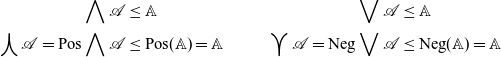
Lemma 1.9 and Corollary 1.8 also imply that these are the tightest such bounds. Suppose there are reducibility candidates $\mathbb{B}$
and
$\mathbb{B}$
and $\mathbb{C}$
such that
$\mathbb{C}$
such that
 \begin{align*} \forall \mathbb{A} \in \mathcal{A}.~ \mathbb{B} &\leq \mathbb{A} & \forall \mathbb{A} \in \mathcal{A}.~ \mathbb{A} &\leq \mathbb{C} \end{align*}
From the lattice properties of $\bigwedge$
and
$\bigwedge$
and $\bigvee$
, monotonicity, and idempotency, we have:
$\bigvee$
, monotonicity, and idempotency, we have:

The other lattice is based on refinement, instead of subtyping. In contrast, the refinement lattice has a opposing relationship with soundness and completeness: one direction of the lattice preserves only soundness, and the other one preserves only completeness.
Definition 1.11 (Refinement Lattice). There is a complete lattice of pre-candidates in ${\mathcal{PC}}$
with respect to refinement order, where the binary intersection (
${\mathcal{PC}}$
with respect to refinement order, where the binary intersection ( $\mathbb{A} \sqcap \mathbb{B}$
a.k.a meet) and union (
$\mathbb{A} \sqcap \mathbb{B}$
a.k.a meet) and union ( $\mathbb{A} \sqcap \mathbb{B}$
, a.k.a join) are defined as:
$\mathbb{A} \sqcap \mathbb{B}$
, a.k.a join) are defined as:
 \begin{align*} \mathbb{A} \sqcap \mathbb{B} &:= (\mathbb{A}^+ \cap \mathbb{B}^+, \mathbb{A}^- \cap \mathbb{B}^-) & \mathbb{A} \sqcup \mathbb{B} &:= (\mathbb{A}^+ \cup \mathbb{B}^+, \mathbb{A}^- \cup \mathbb{B}^-) \end{align*}
Moreover, these generalize to the intersection (
, a.k.a infimum) and union ( $\bigsqcup\mathbb{A}$
, a.k.a supremum) of any set
$\bigsqcup\mathbb{A}$
, a.k.a supremum) of any set $\mathcal{A} \in {\mathcal{PC}}$
of pre-candidates
$\mathcal{A} \in {\mathcal{PC}}$
of pre-candidates

Theorem 1.12 (Sound and Complete Refinement Semi-Lattices). The refinement intersection
![]() forms a meet semi-lattice over sound candidates in
forms a meet semi-lattice over sound candidates in ${\mathcal{SC}}$
, and the refinement union
${\mathcal{SC}}$
, and the refinement union $\bigsqcup$
forms a join semi-lattice over complete candidates in
$\bigsqcup$
forms a join semi-lattice over complete candidates in ${\mathcal{CC}}$
.
${\mathcal{CC}}$
.
Proof Let $\mathcal{A} \in {\mathcal{SC}}$
be a set of sound candidates, i.e., for all
$\mathcal{A} \in {\mathcal{SC}}$
be a set of sound candidates, i.e., for all $\mathbb{A} \in \mathcal{A}$
, we know
$\mathbb{A} \in \mathcal{A}$
, we know $\mathbb{A} \sqsubseteq \mathbb{A}^\unicode{x2AEB}$
. In the refinement lattice on pre-candidates, de Morgan duality (Property 1.13) implies:
$\mathbb{A} \sqsubseteq \mathbb{A}^\unicode{x2AEB}$
. In the refinement lattice on pre-candidates, de Morgan duality (Property 1.13) implies:
So that
is also sound.
Let $\mathcal{A} \in {\mathcal{CC}}$
be a set of complete candidates, i.e., for all
$\mathcal{A} \in {\mathcal{CC}}$
be a set of complete candidates, i.e., for all $\mathbb{A} \in \mathcal{A}$
, we know
$\mathbb{A} \in \mathcal{A}$
, we know $\mathbb{A}^{v\unicode{x2AEB}} \sqsubseteq \mathbb{A}$
. In the refinement lattice on pre-candidates, de Morgan duality (Property 1.13) and the fact that the (co)value restriction
$\mathbb{A}^{v\unicode{x2AEB}} \sqsubseteq \mathbb{A}$
. In the refinement lattice on pre-candidates, de Morgan duality (Property 1.13) and the fact that the (co)value restriction $\rule{1ex}{0.5pt}^v$
distributes over unions implies:
$\rule{1ex}{0.5pt}^v$
distributes over unions implies:
So that $\bigsqcup\mathcal{A}$
is also complete.
$\bigsqcup\mathcal{A}$
is also complete.
Because soundness and completeness are each broken by different directions of this refinement lattice, it doesn’t give us a complete lattice for assembling new reducibility candidates. However, what it does give us is additional insight into the logical properties of orthogonality. That is, while orthogonality behaves like intuitionistic negation, the intersections (
![]() ) and unions (
) and unions ( $\bigsqcup$
) act like conjunction and disjunction, respectively. Together, these give us properties similar to the familiar de Morgan laws of duality intuitionistic logic.
$\bigsqcup$
) act like conjunction and disjunction, respectively. Together, these give us properties similar to the familiar de Morgan laws of duality intuitionistic logic.
Property 1.13 (Orthogonal de Morgan). Given any pre-candidates $\mathbb{A}$
and
$\mathbb{A}$
and $\mathbb{B}$
:
$\mathbb{B}$
:
-
1.
\begin{align*} (\mathbb{A} \sqcup \mathbb{B})^\unicode{x2AEB} = (\mathbb{A}^{\unicode{x2AEB}}) \sqcap (\mathbb{B}^{\unicode{x2AEB}}) . \end{align*}
-
2.
\begin{align*} (\mathbb{A} \sqcap \mathbb{B})^\unicode{x2AEB} \sqsupseteq (\mathbb{A}^{\unicode{x2AEB}}) \sqcup (\mathbb{B}^{\unicode{x2AEB}}) . \end{align*}
-
3.
\begin{align*} (\mathbb{A}^{\unicode{x2AEB}} \sqcap \mathbb{B}^{\unicode{x2AEB}})^{\unicode{x2AEB}\unicode{x2AEB}} = (\mathbb{A}^{\unicode{x2AEB}}) \sqcap (\mathbb{B}^{\unicode{x2AEB}}) = (\mathbb{A} \sqcup \mathbb{B})^{\unicode{x2AEB}} = (\mathbb{A}^{\unicode{x2AEB}\unicode{x2AEB}} \sqcup \mathbb{B}^{\unicode{x2AEB}\unicode{x2AEB}})^\unicode{x2AEB} . \end{align*}


Furthermore, given any set of pre-candidates $\mathcal{A} \subseteq {\mathcal{PC}}$
:
$\mathcal{A} \subseteq {\mathcal{PC}}$
:
-
1.
\begin{align*} (\bigcup\mathcal{A})^\unicode{x2AEB} = \bigcap(\mathcal{A}^{\unicode{x2AEB}*}) . \end{align*}
-
2.
\begin{align*} (\bigcap\mathcal{A})^\unicode{x2AEB} \sqsupseteq \bigcup(\mathcal{A}^{\unicode{x2AEB}*}) . \end{align*}
-
3.
\begin{align*} (\bigcap(\mathcal{A}^{\unicode{x2AEB}*}))^{\unicode{x2AEB}\unicode{x2AEB}} = \bigcap(\mathcal{A}^{\unicode{x2AEB}*}) = \left(\bigcup\mathcal{A}\right)^{\unicode{x2AEB}} = \left(\bigcup\mathcal{A}^{\unicode{x2AEB}*\unicode{x2AEB}*}\right)^{\unicode{x2AEB}} . \end{align*}


Proof We will show only the de Morgan properties for union and intersection over any sets of pre-candidate $\mathcal{A}$
; the binary versions are special cases of these. Note that the union and intersection of the refinement lattice on pre-candidates have these lattice properties:
$\mathcal{A}$
; the binary versions are special cases of these. Note that the union and intersection of the refinement lattice on pre-candidates have these lattice properties:

Taking the contrapositive (Property 1.2) to the facts on the left, and instantiating the facts on the right to $\mathcal{A}^{\unicode{x2AEB}*}$
, gives:
$\mathcal{A}^{\unicode{x2AEB}*}$
, gives:

-
1. We know
$(\bigsqcup\mathcal{A})^\unicode{x2AEB} \sqsubseteq \mathbb{A}^{\unicode{x2AEB}}$
(for each
$\mathbb{A}^{\unicode{x2AEB}} \in \mathcal{A}$
), so
. In the reverse direction, suppose
. For every
$e \in \bigsqcup\mathcal{A}$
, we know there is (at least) one
$\mathbb{A} \in \mathcal{A}$
such that
$e \in \mathbb{A}$
. So since
, we know
$\langle {v} |\!| {e} \rangle \in \unicode{x2AEB}$
by definition of orthogonality (Definition 1.1). Therefore,
$v \in (\bigsqcup\mathcal{A})^\unicode{x2AEB}$
as well. Dually, for every
and
$v \in \bigsqcup\mathcal{A}$
, there it at least one
$v \in \mathbb{A} \in \mathcal{A}$
, forcing
$\langle {v} |\!| {e} \rangle \in \unicode{x2AEB}$
and thus
$e \in (\bigsqcup\mathcal{A})^\unicode{x2AEB}$
. So in general
, making the two sets equal. -
2. We know
(for each
$\mathbb{A}^{\unicode{x2AEB}} \in \mathcal{A}$
), so
. But the reverse direction may not be true:
. Suppose that
. Consider the possibility that each
$\mathbb{A} \in \mathcal{A}$
might contain a term
$v_{\mathbb{A}}$
incompatible with e (i.e.,
$\langle {v_{\mathbb{A}}} |\!| {e} \rangle \notin \unicode{x2AEB}$
), and yet each such
$v_{\mathbb{A}}$
might not end up in the intersection of
$\mathcal{A}$
(
). In this case, e is still orthogonal to every term in
, but there is no individual
$\mathbb{A} \in \mathcal{A}$
such that
$e \in \mathbb{A}^{\unicode{x2AEB}}$
because each one has an associated counter-example
$v_{\mathbb{A}}$
ruling it out. -
3. The last fact follows from the above and triple orthogonal elimination (Property 1.2).


Take note that the missing direction in the asymmetric property (2) ( $(\mathbb{A}\sqcap\mathbb{B})^\unicode{x2AEB} \not\sqsubseteq (\mathbb{A}^\unicode{x2AEB})\sqcup(\mathbb{B}^\unicode{x2AEB})$
) exactly corresponds to the direction of the de Morgan laws which is rejected by intuitionistic logic (the negation of a conjunction does not imply the disjunction of the negations). Instead, we have a weakened version of (2) presented in (3), adding additional applications of orthogonality to restore the symmetric equality rather than an asymmetric refinement. As with other properties like triple orthogonal elimination, this also has a (co)value restricted variant.
$(\mathbb{A}\sqcap\mathbb{B})^\unicode{x2AEB} \not\sqsubseteq (\mathbb{A}^\unicode{x2AEB})\sqcup(\mathbb{B}^\unicode{x2AEB})$
) exactly corresponds to the direction of the de Morgan laws which is rejected by intuitionistic logic (the negation of a conjunction does not imply the disjunction of the negations). Instead, we have a weakened version of (2) presented in (3), adding additional applications of orthogonality to restore the symmetric equality rather than an asymmetric refinement. As with other properties like triple orthogonal elimination, this also has a (co)value restricted variant.
Lemma 1.14 (Restricted de Morgan). For any set of pre-candidates $\mathcal{A} \subseteq {\mathcal{PC}}$
:
$\mathcal{A} \subseteq {\mathcal{PC}}$
:
Proof Follows from the de Morgan laws (Property 1.13), restricted triple orthogonal elimination (Property 1.5), and the fact that the (co)value restriction $\rule{1ex}{0.5pt}^v$
distributes over intersection and unions:
$\rule{1ex}{0.5pt}^v$
distributes over intersection and unions:

With these de Morgan properties of intersection and union, we can be more specific about how the subtype lattice operations $\bigwedge$
and
$\bigwedge$
and $\bigvee$
on pre-candidates are lifted into the complete versions
$\bigvee$
on pre-candidates are lifted into the complete versions
![]() and
and
![]() that form the subtype lattice among reducibility candidates.
that form the subtype lattice among reducibility candidates.
Lemma 1.15. Let $\mathcal{A} \subseteq {\mathcal{RC}}$
be any set of reducibility candidates.
$\mathcal{A} \subseteq {\mathcal{RC}}$
be any set of reducibility candidates.

Proof Follows from de Morgan duality (Property 1.13 and Lemma 1.14) and the fact that reducibility candidates are fixed points of $\rule{1ex}{0.5pt}^{v\unicode{x2AEB}}$
(Lemma 1.6). Let
$\rule{1ex}{0.5pt}^{v\unicode{x2AEB}}$
(Lemma 1.6). Let $\mathcal{A}^+ = \{\mathbb{A}^+ \mid \mathbb{A} \in \mathcal{A}\}$
and
$\mathcal{A}^+ = \{\mathbb{A}^+ \mid \mathbb{A} \in \mathcal{A}\}$
and $\mathcal{A}^- = \{\mathbb{A}^- \mid \mathbb{A} \in \mathcal{A}\}$
in the following:
$\mathcal{A}^- = \{\mathbb{A}^- \mid \mathbb{A} \in \mathcal{A}\}$
in the following:

1.4 (Co)induction and (Co)recursion
We now examine how the (co)inductive types $\operatorname{Nat}$
and
$\operatorname{Nat}$
and $\operatorname{Stream} A$
are properly defined as reducibility candidates in this orthogonality-based, symmetric model. As shorthand, we will use these two functions on reducibility candidates
$\operatorname{Stream} A$
are properly defined as reducibility candidates in this orthogonality-based, symmetric model. As shorthand, we will use these two functions on reducibility candidates
 \begin{align*} N &: {\mathcal{RC}} \to {\mathcal{RC}} & S &: {\mathcal{RC}} \to {\mathcal{RC}} \to {\mathcal{RC}} \\ N(\mathbb{C}) &:= \operatorname{Pos}(\{\operatorname{zero}\} \vee \operatorname{succ}(\mathbb{C})) & S_{\mathbb{A}}(\mathbb{C}) &:= \operatorname{Neg}(\operatorname{head}(\mathbb{A}) \wedge \operatorname{tail}(\mathbb{C}))\end{align*}
defined in terms of these operations that lift constructors and destructors onto candidates:
 \begin{align*} \operatorname{succ}(\mathbb{C}) &:= \{\operatorname{succ} V \mid V \in \mathbb{C}\} & \operatorname{tail}(\mathbb{C}) &:= \{\operatorname{tail} E \mid E \in \mathbb{C}\} & \operatorname{head}(\mathbb{A}) &:= \{\operatorname{head} E \mid E \in \mathbb{A}\}\end{align*}
These capture the (co)inductive steps for the iterative definitions of $[\![ \operatorname{Nat} ]\!]_i$
and
$[\![ \operatorname{Nat} ]\!]_i$
and $[\![ \operatorname{Stream} A ]\!]_i$
:
$[\![ \operatorname{Stream} A ]\!]_i$
:
 \begin{align*} [\![ \operatorname{Nat} ]\!]_{i+1} &= N([\![ \operatorname{Nat} ]\!]_i) & [\![ \operatorname{Stream} A ]\!]_{i+1} &= S_{[\![ A ]\!]}([\![ \operatorname{Stream} A ]\!]_i)\end{align*}
They also capture the all-at-once definitions of $[\![ \operatorname{Nat} ]\!]$
and
$[\![ \operatorname{Nat} ]\!]$
and $[\![ \operatorname{Stream} A ]\!]$
as
$[\![ \operatorname{Stream} A ]\!]$
as
due to the fact that their closure conditions (under $\operatorname{zero},\operatorname{succ},$
and
$\operatorname{zero},\operatorname{succ},$
and $\operatorname{head},\operatorname{tail}$
, respectively) are equivalent to these subtyping conditions.
$\operatorname{head},\operatorname{tail}$
, respectively) are equivalent to these subtyping conditions.
Lemma 1.16. For all reducibility candidates $\mathbb{C}$
-
1.
$N(\mathbb{C}) \leq \mathbb{C}$
if and only if
$\operatorname{zero} \in \mathbb{C}$
and
$\operatorname{succ} V \in \mathbb{C}$
(for all
$V \in \mathbb{C}$
). -
2.
$\mathbb{C} \leq S_{\mathbb{A}}(\mathbb{C})$
if and only if
$\operatorname{head} E \in \mathbb{C}$
(for all
$E \in \mathbb{A}$
) and
$\operatorname{tail} E \in \mathbb{C}$
(for all
$E \in \mathbb{C}$
).


Proof The “only if” directions follow directly from Lemma 6.7 by the definitions of N, $S_{\mathbb{A}}$
, and subtyping. That is, we know that
$S_{\mathbb{A}}$
, and subtyping. That is, we know that $\operatorname{zero} \in N(\mathbb{C})$
and
$\operatorname{zero} \in N(\mathbb{C})$
and $\operatorname{succ} V \in N(\mathbb{C})$
(for all
$\operatorname{succ} V \in N(\mathbb{C})$
(for all $V \in \mathbb{C}$
) by definition of N in terms of
$V \in \mathbb{C}$
) by definition of N in terms of $\operatorname{Pos}$
, and thus, they must be in
$\operatorname{Pos}$
, and thus, they must be in $\mathbb{C} \geq N(\mathbb{C})$
by subtyping. Similarly,
$\mathbb{C} \geq N(\mathbb{C})$
by subtyping. Similarly, $\operatorname{head} E, \operatorname{tail} F \in S_{\mathbb{A}}(\mathbb{C}) \leq \mathbb{C}$
(for all
$\operatorname{head} E, \operatorname{tail} F \in S_{\mathbb{A}}(\mathbb{C}) \leq \mathbb{C}$
(for all $E \in \mathbb{A}$
and
$E \in \mathbb{A}$
and $F \in \mathbb{C}$
) by subtyping and the definition of S in terms of
$F \in \mathbb{C}$
) by subtyping and the definition of S in terms of $\operatorname{Neg}$
.
$\operatorname{Neg}$
.
The “if” direction follows from the universal properties of $\operatorname{Pos}$
and
$\operatorname{Pos}$
and $\operatorname{Neg}$
(Lemma 6.7): for any reducibility candidate
$\operatorname{Neg}$
(Lemma 6.7): for any reducibility candidate $\mathbb{C} \sqsupseteq \mathbb{B}^v$
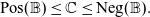 \begin{align*} \operatorname{Pos}(\mathbb{B}) \leq \mathbb{C} \leq \operatorname{Neg}(\mathbb{B}) . \end{align*}
Now note that
 \begin{align*} N(\mathbb{C}) &= \operatorname{Pos}(\{\operatorname{zero}\} \cup \{\operatorname{succ} V \mid V \in \mathbb{C}\},\{\}) \\ S_{\mathbb{A}}(\mathbb{C}) &= \operatorname{Neg} (\{\},\{\operatorname{head} E \mid E \in \mathbb{A}\} \cup \{\operatorname{tail} F \mid F \in \mathbb{C}\}) \end{align*}
Therefore, if $\operatorname{zero} \in \mathbb{C}$
and
$\operatorname{zero} \in \mathbb{C}$
and $\operatorname{succ} V \in \mathbb{C}$
(for all
$\operatorname{succ} V \in \mathbb{C}$
(for all $V \in \mathbb{C}$
) then
$V \in \mathbb{C}$
) then
 \begin{equation*} N(\mathbb{C}) \leq \mathbb{C} \sqsupseteq (\{\operatorname{zero}\} \cup \{\operatorname{succ} V \mid V \in \mathbb{C}\},\{\}) \end{equation*}
Likewise if $\operatorname{head} E \in \mathbb{C}$
and
$\operatorname{head} E \in \mathbb{C}$
and $\operatorname{tail} F \in \mathbb{C}$
(for all
$\operatorname{tail} F \in \mathbb{C}$
(for all $E \in \mathbb{A}$
and
$E \in \mathbb{A}$
and $F \in \mathbb{C}$
) then
$F \in \mathbb{C}$
) then
 \begin{equation*} (\{\},\{\operatorname{head} E \mid E \in \mathbb{A}\} \cup \{\operatorname{tail} F \mid F \in \mathbb{C}\}) \sqsubseteq \mathbb{C} \leq S_{\mathbb{A}}(\mathbb{C}) \end{equation*}
First, consider the model of the $\operatorname{Nat}$
type in terms of the infinite union of approximations:
$\operatorname{Nat}$
type in terms of the infinite union of approximations:
![]() . This reducibility candidate should contain safe instances of the recursor. The reason it does is because the presence of a recursor is preserved by the N stepping operation on reducibility candidates, and so it must remain in the final union
. This reducibility candidate should contain safe instances of the recursor. The reason it does is because the presence of a recursor is preserved by the N stepping operation on reducibility candidates, and so it must remain in the final union
![]() because it is in each approximation
because it is in each approximation $[\![ \operatorname{Nat} ]\!]_i$
.
$[\![ \operatorname{Nat} ]\!]_i$
.
Lemma 1.17 ( $\operatorname{Nat}$
Recursion Step). For any reducibility candidates
$\operatorname{Nat}$
Recursion Step). For any reducibility candidates $\mathbb{B}$
and
$\mathbb{B}$
and $\mathbb{C}$
,
$\mathbb{C}$
,
 \begin{equation*} \operatorname{\mathbf{rec}} \{\operatorname{zero} \to v \mid \operatorname{succ} x \to y.w\} \operatorname{\mathbf{with}} E \in N(\mathbb{C})\end{equation*}
for all $E \in \mathbb{B}$
whenever the following conditions hold:
$E \in \mathbb{B}$
whenever the following conditions hold:
-
$v \in \mathbb{B}$
,
-
$w[{{V}/{x},{W}/{y}}] \in \mathbb{B}$
for all
$V \in \mathbb{C}$
and
$W \in \mathbb{B}$
, and
-
\begin{align*} \operatorname{\mathbf{rec}} \{\operatorname{zero} \to v \mid \operatorname{succ} x \to y.w\} \operatorname{\mathbf{with}} E \in \mathbb{C}\end{align*}
for all
$E \in \mathbb{B}$
.


Proof Note that the accumulator continuation E changes during the successor step, so we will need to generalize over it. As shorthand, let $E^{\operatorname{\mathbf{rec}}}_{E'} := \operatorname{\mathbf{rec}} \{\operatorname{zero} \to v \mid \operatorname{succ} x \to y.w\} \operatorname{\mathbf{with}} E'$
where E’ stands for the given continuation accumulator. It suffices to show (via Corollary 6.9) that for all
$E^{\operatorname{\mathbf{rec}}}_{E'} := \operatorname{\mathbf{rec}} \{\operatorname{zero} \to v \mid \operatorname{succ} x \to y.w\} \operatorname{\mathbf{with}} E'$
where E’ stands for the given continuation accumulator. It suffices to show (via Corollary 6.9) that for all $E' \in \mathbb{B}$
,
$E' \in \mathbb{B}$
, $\langle {\operatorname{zero}} |\!| {E^{\operatorname{\mathbf{rec}}}_{E'}} \rangle$
and
$\langle {\operatorname{zero}} |\!| {E^{\operatorname{\mathbf{rec}}}_{E'}} \rangle$
and $\langle {\operatorname{succ} V} |\!| {E^{\operatorname{\mathbf{rec}}}_{E'}} \rangle$
(for all
$\langle {\operatorname{succ} V} |\!| {E^{\operatorname{\mathbf{rec}}}_{E'}} \rangle$
(for all $V \in \mathbb{C}$
). Observe that, given any
$V \in \mathbb{C}$
). Observe that, given any $E' \in \mathbb{B}$
and
$E' \in \mathbb{B}$
and $V \in \mathbb{C}$
, we have these two possible reductions:
$V \in \mathbb{C}$
, we have these two possible reductions:
Now, we note the following series facts:
-
1.
$\langle {v} |\!| {E'} \rangle \in \unicode{x2AEB}$
because
$v, E' \in \mathbb{B}$
by assumption. -
2.
$w[{{V}/{x},{W}/{y}}] \in \mathbb{B}$
for all
$W \in \mathbb{B}$
because
$V \in \mathbb{C}$
. -
3.
for all
$W \in \mathbb{B}$
. -
4.
by activation (Lemma 6.3). -
5.
$\langle {V} |\!| {E^{\operatorname{\mathbf{rec}}}_{E'}} \rangle \in \unicode{x2AEB}$
for all
$E' \in \mathbb{B}$
by the assumption
$V, E^{\operatorname{\mathbf{rec}}}_{E'} \in \mathbb{C}$
. -
6.
by activation (Lemma 6.3). -
7.


Therefore, $\langle {V} |\!| {E^{\operatorname{\mathbf{rec}}}_{E'}} \rangle$
reduces to a command in
$\langle {V} |\!| {E^{\operatorname{\mathbf{rec}}}_{E'}} \rangle$
reduces to a command in $\unicode{x2AEB}$
for any
$\unicode{x2AEB}$
for any $V \in N(\mathbb{C})$
. It follows from Property 6.4 and Corollary 6.9 that
$V \in N(\mathbb{C})$
. It follows from Property 6.4 and Corollary 6.9 that
 \begin{align*} E^{\operatorname{\mathbf{rec}}}_{E'} \in N(\mathbb{C}) . \end{align*}
Lemma 1.18 ( $\operatorname{Nat}$
Recursion). For any reducibility candidate
$\operatorname{Nat}$
Recursion). For any reducibility candidate $\mathbb{B}$
, if
$\mathbb{B}$
, if
-
$v \in \mathbb{B}$
,
-
$w[{{V}/{x},{W}/{y}}] \in \mathbb{B}$
for all
and
$W \in \mathbb{B}$
, and
-
$E \in \mathbb{B}$
,


then
![]()
Proof By induction on i,
 \begin{align*} \operatorname{\mathbf{rec}} \{\operatorname{zero} \to v \mid \operatorname{succ} x \to y.w\} \operatorname{\mathbf{with}} E' \in [\![ \operatorname{Nat} ]\!]_i \end{align*}
for all
\begin{align*} \operatorname{\mathbf{rec}} \{\operatorname{zero} \to v \mid \operatorname{succ} x \to y.w\} \operatorname{\mathbf{with}} E' \in [\![ \operatorname{Nat} ]\!]_i \end{align*}
for all $E' \in \mathbb{B}$
:
$E' \in \mathbb{B}$
:
(0)
$[\![ \operatorname{Nat} ]\!]_0 = \operatorname{Pos}\{\}$
is the least reducibility candidate w.r.t subtyping, i.e., with the fewest terms and the most coterms, so
$\operatorname{\mathbf{rec}} \{\operatorname{zero} \to v \mid \operatorname{succ} x \to y.w\} \operatorname{\mathbf{with}} E' \in [\![ \operatorname{Nat} ]\!]_0$
trivially.(
$i+1$
) Assume the inductive hypothesis:
\begin{align*} \operatorname{\mathbf{rec}} \{\operatorname{zero} \to v \mid \operatorname{succ} x \to y.w\} \operatorname{\mathbf{with}} E' \in [\![ \operatorname{Nat} ]\!]_i \end{align*}
for all
$E' \in \mathbb{B}$
. Applying Lemma 1.17 to
$[\![ \operatorname{Nat} ]\!]_i$
, we have (for all
$E' \in \mathbb{B}$
):
\begin{align*} \operatorname{\mathbf{rec}} \{\operatorname{zero} \to v \mid \operatorname{succ} x \to y.w\} \operatorname{\mathbf{with}} E' \in N([\![ \operatorname{Nat} ]\!]_{i+1}) = [\![ \operatorname{Nat} ]\!]_{i+1} \end{align*}


Thus, we know that the least upper bound of all $[\![ \operatorname{Nat} ]\!]_i$
in the subtype lattice (Theorem 6.10) contains the instance of this recursor with
$[\![ \operatorname{Nat} ]\!]_i$
in the subtype lattice (Theorem 6.10) contains the instance of this recursor with $E' = E \in \mathbb{B}$
because it is a covalue (Lemma 6.7):
$E' = E \in \mathbb{B}$
because it is a covalue (Lemma 6.7):

Showing that the union
![]() is closed under the
is closed under the $\operatorname{succ}$
constructor is more difficult. The simple union
$\operatorname{succ}$
constructor is more difficult. The simple union $\bigvee_{i=0}^\infty[\![ \operatorname{Nat} ]\!]_i$
is clearly closed under
$\bigvee_{i=0}^\infty[\![ \operatorname{Nat} ]\!]_i$
is clearly closed under $\operatorname{succ}$
: every value in
$\operatorname{succ}$
: every value in $\bigvee_{i=0}^\infty[\![ \operatorname{Nat} ]\!]_i$
must come from some individual approximation
$\bigvee_{i=0}^\infty[\![ \operatorname{Nat} ]\!]_i$
must come from some individual approximation $[\![ \operatorname{Nat} ]\!]_n$
, so its successor is in the next one
$[\![ \operatorname{Nat} ]\!]_n$
, so its successor is in the next one $[\![ \operatorname{Nat} ]\!]_{n+1}$
. However,
$[\![ \operatorname{Nat} ]\!]_{n+1}$
. However,
![]() is not just a simple union; it has been completed by
is not just a simple union; it has been completed by $\operatorname{Pos}$
, so it might—hypothetically—contain more terms which do not come from any individual
$\operatorname{Pos}$
, so it might—hypothetically—contain more terms which do not come from any individual $[\![ \operatorname{Nat} ]\!]_n$
. Thankfully, this does not happen. It turns out the two unions are one in the same—the
$[\![ \operatorname{Nat} ]\!]_n$
. Thankfully, this does not happen. It turns out the two unions are one in the same—the $\operatorname{Pos}$
completion cannot add anything more because of infinite recursors which can inspect numbers of any size—which lets us show that
$\operatorname{Pos}$
completion cannot add anything more because of infinite recursors which can inspect numbers of any size—which lets us show that
![]() is indeed closed under
is indeed closed under $\operatorname{succ}$
.
$\operatorname{succ}$
.
Lemma 1.19 (Nat Choice).
![]()
Proof We already know that
![]() by definition (since all reducibility candidates are pre-candidates), so it suffices to show the reverse:
by definition (since all reducibility candidates are pre-candidates), so it suffices to show the reverse:
![]() .
.
Note from Lemma 1.15 that
We will proceed by showing there is an $E \in \bigvee_{i=0}^\infty[\![ \operatorname{Nat} ]\!]_i$
such that
$E \in \bigvee_{i=0}^\infty[\![ \operatorname{Nat} ]\!]_i$
such that $[\![ {V} |\!| {E} ]\!] \in \unicode{x2AEB}$
forces
$[\![ {V} |\!| {E} ]\!] \in \unicode{x2AEB}$
forces $V \in \bigvee_{i=0}^\infty[\![ \operatorname{Nat} ]\!]_i$
. Since we know that every
$V \in \bigvee_{i=0}^\infty[\![ \operatorname{Nat} ]\!]_i$
. Since we know that every
and $E \in \bigvee_{i=0}^\infty[\![ \operatorname{Nat} ]\!]_i$
forms a safe command
$E \in \bigvee_{i=0}^\infty[\![ \operatorname{Nat} ]\!]_i$
forms a safe command $\langle {V} |\!| {E} \rangle \in \unicode{x2AEB}$
, this proves the result.
$\langle {V} |\!| {E} \rangle \in \unicode{x2AEB}$
, this proves the result.
First, observe that
contains the following instance of the recursor (Lemma 1.18):

which has these reductions with $\operatorname{zero}$
and
$\operatorname{zero}$
and $\operatorname{succ}$
:
$\operatorname{succ}$
:
The reason why this covalue forces values of
into values of $\bigvee_{i=0}^\infty[\![ \operatorname{Nat} ]\!]_i$
depends on the evaluation strategy.
$\bigvee_{i=0}^\infty[\![ \operatorname{Nat} ]\!]_i$
depends on the evaluation strategy.
In call-by-value, the first successor reduction proceeds as:
 \begin{align*} \langle {\operatorname{succ} V} |\!| {\operatorname{\mathbf{rec}}_\infty} \rangle &\mathrel{\mapsto\!\!\!\!\to} \langle {V} |\!| {\operatorname{\mathbf{rec}}_\infty[{{{\tilde{\mu}}{x}. \langle {x} |\!| {\alpha} \rangle}/{\alpha}}]} \rangle \end{align*}
where the continuation accumulator has been ${\tilde{\mu}}$
-expanded. In general, an arbitrary step in this reduction sequence looks like:
${\tilde{\mu}}$
-expanded. In general, an arbitrary step in this reduction sequence looks like:
 \begin{align*} \langle {\operatorname{succ} V} |\!| {\operatorname{\mathbf{rec}}_\infty[{{E}/{\alpha}}]} \rangle &\mathrel{\mapsto\!\!\!\!\to} \langle {V} |\!| {\operatorname{\mathbf{rec}}_\infty[{{{\tilde{\mu}}{x}. \langle {x} |\!| {E} \rangle}/{\alpha}}]} \rangle \end{align*}
The only values (in call-by-value) which do not get stuck with $\operatorname{\mathbf{rec}}_\infty$
(i.e., values V such that
$\operatorname{\mathbf{rec}}_\infty$
(i.e., values V such that $\langle {V} |\!| {\operatorname{\mathbf{rec}}_\infty} \rangle \mathrel{\mapsto\!\!\!\!\to} c \in \mathit{Final}$
) have the form
$\langle {V} |\!| {\operatorname{\mathbf{rec}}_\infty} \rangle \mathrel{\mapsto\!\!\!\!\to} c \in \mathit{Final}$
) have the form $\operatorname{succ}^n \operatorname{zero}$
which is in
$\operatorname{succ}^n \operatorname{zero}$
which is in
![]() .
.
In call-by-name, the successor reduction proceeds as:
 \begin{align*} \langle {\operatorname{succ} V} |\!| {\operatorname{\mathbf{rec}}_\infty} \rangle &\mathrel{\mapsto\!\!\!\!\to} \langle {V} |\!| {\operatorname{\mathbf{rec}}_\infty} \rangle \end{align*}
Call-by-name includes another form of value, $\mu{\beta}. c$
, which is not immediately stuck with
$\mu{\beta}. c$
, which is not immediately stuck with $\operatorname{\mathbf{rec}}_\infty$
. We now need to show that
$\operatorname{\mathbf{rec}}_\infty$
. We now need to show that $\langle {V} |\!| {\operatorname{\mathbf{rec}}_\infty} \rangle \in \unicode{x2AEB}$
, i.e.,
$\langle {V} |\!| {\operatorname{\mathbf{rec}}_\infty} \rangle \in \unicode{x2AEB}$
, i.e., $\langle {V} |\!| {\operatorname{\mathbf{rec}}_\infty} \rangle \mathrel{\mapsto\!\!\!\!\to} c \in \mathit{Final}$
, forces
$\langle {V} |\!| {\operatorname{\mathbf{rec}}_\infty} \rangle \mathrel{\mapsto\!\!\!\!\to} c \in \mathit{Final}$
, forces $V \in [\![ \operatorname{Nat} ]\!]_n$
for some n. Let’s examine this reduction more closely and check the intermediate results by abstracting out
$V \in [\![ \operatorname{Nat} ]\!]_n$
for some n. Let’s examine this reduction more closely and check the intermediate results by abstracting out $\operatorname{\mathbf{rec}}_\infty$
with a fresh covariable
$\operatorname{\mathbf{rec}}_\infty$
with a fresh covariable $\beta$
:
$\beta$
: $\langle {V} |\!| {\operatorname{\mathbf{rec}}_\infty} \rangle \mathrel{\mapsto\!\!\!\!\to} c \in \mathit{Final}$
because
$\langle {V} |\!| {\operatorname{\mathbf{rec}}_\infty} \rangle \mathrel{\mapsto\!\!\!\!\to} c \in \mathit{Final}$
because $\langle {V} |\!| {\operatorname{\mathbf{rec}}_\infty} \rangle \mathrel{\mapsto\!\!\!\!\to} c'[{{\operatorname{\mathbf{rec}}_\infty}/{\beta}}]$
for some
$\langle {V} |\!| {\operatorname{\mathbf{rec}}_\infty} \rangle \mathrel{\mapsto\!\!\!\!\to} c'[{{\operatorname{\mathbf{rec}}_\infty}/{\beta}}]$
for some $\langle {V} |\!| {\beta} \rangle \mathrel{\mapsto\!\!\!\!\to} c' \not\mapsto$
and then
$\langle {V} |\!| {\beta} \rangle \mathrel{\mapsto\!\!\!\!\to} c' \not\mapsto$
and then $c'[{{\operatorname{\mathbf{rec}}_\infty}/{\beta}}] \mathrel{\mapsto\!\!\!\!\to} c \in \mathit{Final}$
. We now proceed by (strong) induction on the length of the remaining reduction sequence (i.e., the number of steps in
$c'[{{\operatorname{\mathbf{rec}}_\infty}/{\beta}}] \mathrel{\mapsto\!\!\!\!\to} c \in \mathit{Final}$
. We now proceed by (strong) induction on the length of the remaining reduction sequence (i.e., the number of steps in $c'[{{\operatorname{\mathbf{rec}}_\infty}/{\beta}}] \mathrel{\mapsto\!\!\!\!\to} c$
) and by cases on the shape of the intermediate c’:
$c'[{{\operatorname{\mathbf{rec}}_\infty}/{\beta}}] \mathrel{\mapsto\!\!\!\!\to} c$
) and by cases on the shape of the intermediate c’:
-
$c' \neq \langle {W} |\!| {\beta} \rangle$
. Then,
\begin{align*} c'[{{\operatorname{\mathbf{rec}}_\infty}/{\beta}}] \in \mathit{Final} \end{align*}
already. In this case,
$\langle {W} |\!| {E} \rangle \in \unicode{x2AEB}$
for any E whatsoever by expansion (Property 6.4), and so
$W \in [\![ \operatorname{Nat} ]\!]_0 = \operatorname{Pos}\{\}$
.
-
$c' = \langle {W} |\!| {\beta} \rangle$
. Then we know that
\begin{align*} c'[{{\operatorname{\mathbf{rec}}_\infty}/{\beta}}] = \langle {W[{{\operatorname{\mathbf{rec}}_\infty}/{\beta}}]} |\!| {\operatorname{\mathbf{rec}}_\infty} \rangle \mathrel{\mapsto\!\!\!\!\to} c \in \mathit{Final} . \end{align*}
Since
$\langle {W} |\!| {\beta} \rangle \not\mapsto$
we know
$W[{{\operatorname{\mathbf{rec}}_\infty}/{\beta}}]$
is not a
$\mu$
-abstraction. The only other possibilities for
$W[{{\operatorname{\mathbf{rec}}_\infty}/{\beta}}]$
, given the known reduction to c, are
$\operatorname{zero}$
or
$\operatorname{succ} V'$
for some V’.
by definition. In the case of
$\operatorname{succ} V'$
, we have the (non-reflexive) reduction sequence
\begin{align*} c'[{{\operatorname{\mathbf{rec}}_\infty}/{\beta}}] = \langle {\operatorname{succ} V'} |\!| {\operatorname{\mathbf{rec}}_\infty} \rangle \mathrel{\mapsto\!\!\!\!\to} \langle {V'} |\!| {\operatorname{\mathbf{rec}}_\infty} \rangle \mathrel{\mapsto\!\!\!\!\to} c . \end{align*}
The inductive hypothesis on the smaller reduction
$\langle {V'} |\!| {\operatorname{\mathbf{rec}}_\infty} \rangle \mathrel{\mapsto\!\!\!\!\to} c$
ensures
$V' \in [\![ \operatorname{Nat} ]\!]_n$
for some n, so that
$\operatorname{succ} V' \in [\![ \operatorname{Nat} ]\!]_{n+1}$
by definition, and thus
$V \in [\![ \operatorname{Nat} ]\!]_{n+1}$
as well by expansion.


So in both call-by-value and call-by-name, we have
 \begin{align*} \left(\bigcap_{i=0}^\infty[\![ \operatorname{Nat} ]\!]_i^-\right)^{v\unicode{x2AEB}} \subseteq \bigcup_{i=0}^\infty[\![ \operatorname{Nat} ]\!]_i^+ . \end{align*}
De Morgan duality (Lemma 1.6) ensures the reverse, so
\begin{align*} \left(\bigcap_{i=0}^\infty[\![ \operatorname{Nat} ]\!]_i^-\right)^{v\unicode{x2AEB}} \subseteq \bigcup_{i=0}^\infty[\![ \operatorname{Nat} ]\!]_i^+ . \end{align*}
De Morgan duality (Lemma 1.6) ensures the reverse, so
 \begin{align*} \left(\bigcap_{i=0}^\infty[\![ \operatorname{Nat} ]\!]_i^-\right)^{v\unicode{x2AEB}} = \bigcup_{i=0}^\infty[\![ \operatorname{Nat} ]\!]_i^+ . \end{align*}
Finally, because all reducibility candidates are fixed points of
\begin{align*} \left(\bigcap_{i=0}^\infty[\![ \operatorname{Nat} ]\!]_i^-\right)^{v\unicode{x2AEB}} = \bigcup_{i=0}^\infty[\![ \operatorname{Nat} ]\!]_i^+ . \end{align*}
Finally, because all reducibility candidates are fixed points of $\rule{1ex}{0.5pt}^{v\unicode{x2AEB}}$
(Lemma 1.6), de Morgan duality further implies:
$\rule{1ex}{0.5pt}^{v\unicode{x2AEB}}$
(Lemma 1.6), de Morgan duality further implies:

Due to the symmetry of the model, the story for $\operatorname{Stream} A$
is very much the same as
$\operatorname{Stream} A$
is very much the same as $\operatorname{Nat}$
. We can show that the intersection of approximations—
$\operatorname{Nat}$
. We can show that the intersection of approximations—
![]() —contains safe instances of the corecursor because its presence is preserved by the stepping function S. The task of showing that this intersection is closed under the
—contains safe instances of the corecursor because its presence is preserved by the stepping function S. The task of showing that this intersection is closed under the $\operatorname{tail}$
destructor is more challenging in the same way as
$\operatorname{tail}$
destructor is more challenging in the same way as $\operatorname{succ}$
closure. We solve it with the dual method: the presence of corecursors which “inspect” stream continuations of any size ensures that there are no new surprises that are not already found in one of the approximations
$\operatorname{succ}$
closure. We solve it with the dual method: the presence of corecursors which “inspect” stream continuations of any size ensures that there are no new surprises that are not already found in one of the approximations $[\![ \operatorname{Stream} A ]\!]_n$
.
$[\![ \operatorname{Stream} A ]\!]_n$
.
Lemma 1.20 ( $\operatorname{Stream}$
Corecursion Step). For any reducibility candidates
$\operatorname{Stream}$
Corecursion Step). For any reducibility candidates $\mathbb{A}$
,
$\mathbb{A}$
, $\mathbb{B}$
and
$\mathbb{B}$
and $\mathbb{C}$
,
$\mathbb{C}$
,
 \begin{align*} \operatorname{\mathbf{corec}} \{\operatorname{head}\alpha \to e \mid \operatorname{tail}\beta \to \gamma.f\} \operatorname{\mathbf{with}} V \in S_{\mathbb{A}}(\mathbb{C})\end{align*}
for all $V \in \mathbb{B}$
whenever the following conditions hold:
$V \in \mathbb{B}$
whenever the following conditions hold:
-
$e[{{E}/{\alpha}}] \in \mathbb{B}$
for all
$E \in \mathbb{A}$
,
-
$f[{{E}/{\beta},{F}/{\gamma}}] \in \mathbb{B}$
for all
$E \in \mathbb{C}$
and
$F \in \mathbb{B}$
, and
-
\begin{align*} \operatorname{\mathbf{corec}} \{\operatorname{head}\alpha \to e \mid \operatorname{tail}\beta \to \gamma.f\} \operatorname{\mathbf{with}} V \in \mathbb{C} \end{align*}
for all
$V \in \mathbb{B}$
.


Proof Since the value accumulator V will change in the tail step, we have to generalize over it. Let
 \begin{align*} V^{\operatorname{\mathbf{corec}}}_{V} := \operatorname{\mathbf{corec}} \{\operatorname{head}\alpha \to e \mid \operatorname{tail}\beta \to \gamma.f\} \operatorname{\mathbf{with}} V , \end{align*}
where V stands for a given value from
\begin{align*} V^{\operatorname{\mathbf{corec}}}_{V} := \operatorname{\mathbf{corec}} \{\operatorname{head}\alpha \to e \mid \operatorname{tail}\beta \to \gamma.f\} \operatorname{\mathbf{with}} V , \end{align*}
where V stands for a given value from $\mathbb{B}$
. It suffices to show (via Corollary 6.9) that for all
$\mathbb{B}$
. It suffices to show (via Corollary 6.9) that for all $V \in \mathbb{B}$
,
$V \in \mathbb{B}$
, $\langle {V^{\operatorname{\mathbf{corec}}}_{V}} |\!| {\operatorname{head} E} \rangle$
(for all
$\langle {V^{\operatorname{\mathbf{corec}}}_{V}} |\!| {\operatorname{head} E} \rangle$
(for all $E \in \mathbb{A}$
) and
$E \in \mathbb{A}$
) and $\langle {V^{\operatorname{\mathbf{corec}}}_{V}} |\!| {\operatorname{tail} E'} \rangle$
(for all
$\langle {V^{\operatorname{\mathbf{corec}}}_{V}} |\!| {\operatorname{tail} E'} \rangle$
(for all $E' \in \mathbb{C}$
). We have these two possible reductions:
$E' \in \mathbb{C}$
). We have these two possible reductions:
Now, we note the following series of facts
-
1.
$e[{{E}/{\alpha}}] \in \mathbb{B}$
by assumption because
$E \in \mathbb{A}$
. -
2.
$\langle {V} |\!| {e[{{E}/{\alpha}}]} \rangle \in \unicode{x2AEB}$
because
$V, e[{{E}/{\alpha}}] \in \mathbb{B}$
by assumption. -
3.
$f[{{E'}/{\beta},{F}/{\gamma}}] \in \mathbb{B}$
for all
$F \in \mathbb{B}$
by because
\begin{align*} E' \in \mathbb{C} . \end{align*}
-
4.
$\langle {V} |\!| {f[{{E'}/{\beta},{F}/{\gamma}}]} \rangle \in \unicode{x2AEB}$
for all
$F \in \mathbb{B}$
. -
5.
$\mu{\gamma}.\langle {V} |\!| {f[{{E'}/{\beta}}]} \rangle \in \mathbb{B}$
by activation (Lemma 6.3). -
6.
$\langle {V^{\operatorname{\mathbf{corec}}}_{V'}} |\!| {E'} \rangle \in \unicode{x2AEB}$
for all
$V' \in \mathbb{B}$
by the inductive hypothesis since
$E' \in [\![ \operatorname{Stream} A ]\!]_i$
. -
7.
${\tilde{\mu}}{x}. \langle {V^{\operatorname{\mathbf{corec}}}_x} |\!| {E'} \rangle \in \mathbb{B}$
by activation (Lemma 6.3). -
8.


Therefore, both $\langle {V^{\operatorname{\mathbf{corec}}}_{V}} |\!| {\operatorname{head} E} \rangle$
and
$\langle {V^{\operatorname{\mathbf{corec}}}_{V}} |\!| {\operatorname{head} E} \rangle$
and $\langle {V^{\operatorname{\mathbf{corec}}}_{V}} |\!| {\operatorname{tail} E'} \rangle$
reduce to a command in
$\langle {V^{\operatorname{\mathbf{corec}}}_{V}} |\!| {\operatorname{tail} E'} \rangle$
reduce to a command in $\unicode{x2AEB}$
for any
$\unicode{x2AEB}$
for any $E \in \mathbb{A}$
and
$E \in \mathbb{A}$
and $E' \in \mathbb{C}$
. It follows from Property 6.4 and Corollary 6.9 that
$E' \in \mathbb{C}$
. It follows from Property 6.4 and Corollary 6.9 that
 \begin{align*} V^{\operatorname{\mathbf{corec}}}_{V'} \in S_{\mathbb{A}}(\mathbb{C}) . \end{align*}
Lemma 1.21 ( $\operatorname{Stream}$
Correcursion). For any reducibility candidate
$\operatorname{Stream}$
Correcursion). For any reducibility candidate $\mathbb{B}$
, if
$\mathbb{B}$
, if
-
$e[{{E}/{\alpha}}] \in \mathbb{B}$
for all
$E \in [\![ A ]\!]$
,
-
$f[{{E}/{\beta},{F}/{\gamma}}] \in \mathbb{B}$
for all
and
$F \in \mathbb{B}$
, and
-
$V \in \mathbb{B}$
,


then
![]()
Proof By induction on i,
 \begin{align*} \operatorname{\mathbf{corec}} \{\operatorname{head}\alpha \to e \mid \operatorname{tail}\beta \to \gamma.f\} \operatorname{\mathbf{with}} V' \in [\![ \operatorname{Stream} A ]\!]_i \end{align*}
for all
\begin{align*} \operatorname{\mathbf{corec}} \{\operatorname{head}\alpha \to e \mid \operatorname{tail}\beta \to \gamma.f\} \operatorname{\mathbf{with}} V' \in [\![ \operatorname{Stream} A ]\!]_i \end{align*}
for all $V' \in \mathbb{B}$
:
$V' \in \mathbb{B}$
:
(0)
$[\![ \operatorname{Stream} A ]\!]_0 = \operatorname{Neg}\{\}$
is the greatest reducibility candidate w.r.t subtyping, i.e., with the most terms, so
\begin{align*} \operatorname{\mathbf{corec}} \{\operatorname{head}\alpha \to e \mid \operatorname{tail}\beta \to \gamma.f\} \operatorname{\mathbf{with}} V' \in [\![ \operatorname{Stream} A ]\!]_0 \end{align*}
trivially.(
$i+1$
) Assume
\begin{align*} \operatorname{\mathbf{corec}} \{\operatorname{head}\alpha \to e \mid \operatorname{tail}\beta \to \gamma.f\} \operatorname{\mathbf{with}} V' \in [\![ \operatorname{Stream} A ]\!]_i \end{align*}
for all
$V' \in \mathbb{B}$
. Applying Lemma 1.20 to
$\mathbb{\operatorname{Stream} A}_i$
, we have (for all
$V' \in \mathbb{B}$
):
\begin{equation*} \operatorname{\mathbf{corec}} \{\operatorname{head}\alpha \to e \mid \operatorname{tail}\beta \to \gamma.f\} \operatorname{\mathbf{with}} V' \in S_{[\![ A ]\!]}(\operatorname{tail}[\![ \operatorname{Stream} A ]\!]_i) = [\![ \operatorname{Stream} A ]\!]_{i+1} \end{equation*}


Thus, we know that in the greatest lower bound of all $[\![ \operatorname{Stream} A ]\!]_i$
in the subtype lattice (Theorem 6.10) contains this corecursor with
$[\![ \operatorname{Stream} A ]\!]_i$
in the subtype lattice (Theorem 6.10) contains this corecursor with $V' = V \in \mathbb{B}$
because it is a value (Lemma 6.7):
$V' = V \in \mathbb{B}$
because it is a value (Lemma 6.7):

Lemma 1.22 (Stream Choice).
![]()
Proof In the special case that $[\![ A ]\!]$
is somehow completely empty of values, it must be the least candidate (w.r.t. subtyping), which also makes each
$[\![ A ]\!]$
is somehow completely empty of values, it must be the least candidate (w.r.t. subtyping), which also makes each $[\![ \operatorname{Stream} A ]\!]_i$
the least candidate as well, forcing
$[\![ \operatorname{Stream} A ]\!]_i$
the least candidate as well, forcing
![]() and
and $\bigwedge_{i=0}^\infty[\![\operatorname{Stream}{A}]\!]_i$
to both be equal to the least candidate and thus equal to each other. Otherwise, we may assume that
$\bigwedge_{i=0}^\infty[\![\operatorname{Stream}{A}]\!]_i$
to both be equal to the least candidate and thus equal to each other. Otherwise, we may assume that $[\![ A ]\!]$
contains at least one value.
$[\![ A ]\!]$
contains at least one value.
Note from Lemma 1.15 that
We will proceed by showing there is a $V \in \bigwedge_{i=0}^\infty[\![ \operatorname{Stream} A ]\!]_i$
such that
$V \in \bigwedge_{i=0}^\infty[\![ \operatorname{Stream} A ]\!]_i$
such that $\langle {V} |\!| {E} \rangle \in \unicode{x2AEB}$
forces
$\langle {V} |\!| {E} \rangle \in \unicode{x2AEB}$
forces $E \in \bigwedge_{i=0}^\infty[\![ \operatorname{Stream} A ]\!]_i$
. Since we know that every
$E \in \bigwedge_{i=0}^\infty[\![ \operatorname{Stream} A ]\!]_i$
. Since we know that every
and $V \in \bigwedge_{i=0}^\infty[\![ \operatorname{Stream} A ]\!]_i$
forms a safe command
$V \in \bigwedge_{i=0}^\infty[\![ \operatorname{Stream} A ]\!]_i$
forms a safe command $\langle {V} |\!| {E} \rangle \in \unicode{x2AEB}$
, this proves the result.
$\langle {V} |\!| {E} \rangle \in \unicode{x2AEB}$
, this proves the result.
First, we define the following corecursive term:
 \begin{align*} \operatorname{\mathbf{corec}}_\infty[V] &:= \operatorname{\mathbf{corec}} \{\operatorname{head} \alpha \to \alpha \to \operatorname{tail} \rule{1ex}{0.5pt} \to \gamma. \gamma\} \operatorname{\mathbf{with}} V \end{align*}
and observe that
(Lemma 1.21) for all $V \in [\![ A ]\!]$
. In general,
$V \in [\![ A ]\!]$
. In general, $\operatorname{\mathbf{corec}}_\infty[V]$
has these reductions with
$\operatorname{\mathbf{corec}}_\infty[V]$
has these reductions with $\operatorname{head}$
and
$\operatorname{head}$
and $\operatorname{tail}$
:
$\operatorname{tail}$
:
The reason why this value forces covalues of
into covalues of $\bigwedge_{i=0}^\infty[\![ \operatorname{Stream} A ]\!]_i$
depends on the evaluation strategy.
$\bigwedge_{i=0}^\infty[\![ \operatorname{Stream} A ]\!]_i$
depends on the evaluation strategy.
In call-by-name, the tail reduction proceeds as:
 \begin{align*} \langle {\operatorname{\mathbf{corec}}_\infty[V]} |\!| {\operatorname{tail} E} \rangle &\mathrel{\mapsto\!\!\!\!\to} \langle {\operatorname{\mathbf{corec}}_\infty[\mu{\gamma}. \langle {V} |\!| {\gamma} \rangle]} |\!| {E} \rangle \end{align*}
where the value accumulator has been $\mu$
-expanded. The only covalues (in call-by-name) which do not get stuck with
$\mu$
-expanded. The only covalues (in call-by-name) which do not get stuck with $\operatorname{\mathbf{corec}}_\infty$
(i.e., covalues E such that
$\operatorname{\mathbf{corec}}_\infty$
(i.e., covalues E such that $\langle {\operatorname{\mathbf{corec}}_\infty[V]} |\!| {E} \rangle \mathrel{\mapsto\!\!\!\!\to} c \in \mathit{Final}$
) have the form
$\langle {\operatorname{\mathbf{corec}}_\infty[V]} |\!| {E} \rangle \mathrel{\mapsto\!\!\!\!\to} c \in \mathit{Final}$
) have the form $\operatorname{tail}^n (\operatorname{head} E)$
with
$\operatorname{tail}^n (\operatorname{head} E)$
with $E \in [\![ A ]\!]$
, which is in
$E \in [\![ A ]\!]$
, which is in
![]() .
.
In call-by-value, the tail reduction proceeds as:
 \begin{align*} \langle {\operatorname{\mathbf{corec}}_\infty[V]} |\!| {\operatorname{tail} E} \rangle &\mathrel{\mapsto\!\!\!\!\to} \langle {\operatorname{\mathbf{corec}}_\infty[V]} |\!| {E} \rangle \end{align*}
Call-by-value includes another form of covalue, ${\tilde{\mu}}{y}. c$
, which is not immediately stuck with
${\tilde{\mu}}{y}. c$
, which is not immediately stuck with $\operatorname{\mathbf{corec}}_\infty$
. We now need to show that if
$\operatorname{\mathbf{corec}}_\infty$
. We now need to show that if $V \in [\![ A ]\!]$
then
$V \in [\![ A ]\!]$
then $\langle {\operatorname{\mathbf{corec}}_\infty[V]} |\!| {E} \rangle \in \unicode{x2AEB}$
, i.e.,
$\langle {\operatorname{\mathbf{corec}}_\infty[V]} |\!| {E} \rangle \in \unicode{x2AEB}$
, i.e., $\langle {\operatorname{\mathbf{corec}}_\infty[V]} |\!| {E} \rangle \mathrel{\mapsto\!\!\!\!\to} c \in \mathit{Final}$
, forces
$\langle {\operatorname{\mathbf{corec}}_\infty[V]} |\!| {E} \rangle \mathrel{\mapsto\!\!\!\!\to} c \in \mathit{Final}$
, forces $E \in [\![ \operatorname{Stream} A ]\!]_n$
for some n. Let’s look at the intermediate results of this reduction sequence by abstracting out
$E \in [\![ \operatorname{Stream} A ]\!]_n$
for some n. Let’s look at the intermediate results of this reduction sequence by abstracting out $\operatorname{\mathbf{corec}}_\infty$
with a fresh variable y:
$\operatorname{\mathbf{corec}}_\infty$
with a fresh variable y: $\langle {\operatorname{\mathbf{corec}}_\infty[V]} |\!| {E} \rangle \mathrel{\mapsto\!\!\!\!\to} c$
because
$\langle {\operatorname{\mathbf{corec}}_\infty[V]} |\!| {E} \rangle \mathrel{\mapsto\!\!\!\!\to} c$
because $\langle {\operatorname{\mathbf{corec}}_\infty[V]} |\!| {E} \rangle \mathrel{\mapsto\!\!\!\!\to} c'[{{\operatorname{\mathbf{corec}}_\infty[V]}/{y}}]$
for some
$\langle {\operatorname{\mathbf{corec}}_\infty[V]} |\!| {E} \rangle \mathrel{\mapsto\!\!\!\!\to} c'[{{\operatorname{\mathbf{corec}}_\infty[V]}/{y}}]$
for some $\langle {y} |\!| {E} \rangle \mathrel{\mapsto\!\!\!\!\to} c' \not\mapsto$
and then
$\langle {y} |\!| {E} \rangle \mathrel{\mapsto\!\!\!\!\to} c' \not\mapsto$
and then $c'[{{\operatorname{\mathbf{corec}}_\infty[V]}/{y}}] \mathrel{\mapsto\!\!\!\!\to} c \in \mathit{Final}$
. We now proceed by (strong) induction on the length of the remain reduction sequence (i.e., the number of steps in
$c'[{{\operatorname{\mathbf{corec}}_\infty[V]}/{y}}] \mathrel{\mapsto\!\!\!\!\to} c \in \mathit{Final}$
. We now proceed by (strong) induction on the length of the remain reduction sequence (i.e., the number of steps in $c'[{{\operatorname{\mathbf{corec}}_\infty[V]}/{y}}] \mathrel{\mapsto\!\!\!\!\to} c$
) and by cases on the shape of the intermediate c’:
$c'[{{\operatorname{\mathbf{corec}}_\infty[V]}/{y}}] \mathrel{\mapsto\!\!\!\!\to} c$
) and by cases on the shape of the intermediate c’:
-
$c' \neq \langle {y} |\!| {F} \rangle$
. Then,
$c'[{{\operatorname{\mathbf{corec}}_\infty[V]}/{y}}] \in \mathit{Final}$
already. In this case,
$\langle {W} |\!| {F} \rangle \in \unicode{x2AEB}$
for any W whatsoever by expansion (Property 6.4), and so
$F \in [\![ \operatorname{Stream} A ]\!]_0 = \operatorname{Neg}\{\}$
.
-
$c' = \langle {y} |\!| {F} \rangle$
. Then,
\begin{align*} c'[{{\operatorname{\mathbf{corec}}_\infty[V]}/{y}}] = \langle {\operatorname{\mathbf{corec}}_\infty[V]} |\!| {F[{{\operatorname{\mathbf{corec}}_\infty[V]}/{y}}]} \rangle \mathrel{\mapsto\!\!\!\!\to} c \in \mathit{Final} . \end{align*}
Since
$\langle {y} |\!| {F} \rangle \not\mapsto$
, we know
$F[{{\operatorname{\mathbf{corec}}_\infty[V]}/{y}}]$
is not a
${\tilde{\mu}}$
-abstraction. The only other possibilities for
$F[{{\operatorname{\mathbf{corec}}_\infty[V]}/{y}}]$
, given the known reduction to c, are
$\operatorname{head} F'$
or
$\operatorname{tail} E'$
. In the first case, we have
\begin{align*} \langle {\operatorname{\mathbf{corec}}_\infty[V]} |\!| {\operatorname{head} F'} \rangle \mapsto \langle {V} |\!| {F'} \rangle \in \unicode{x2AEB} \end{align*}
for all
$V \in [\![ A ]\!]$
; so
$F' \in [\![ A ]\!]$
by completion of
$[\![ A ]\!]$
and thus
$\operatorname{head} F' \in [\![ \operatorname{Stream} A ]\!]_1$
. In the second case, we have the (non-reflexive) reduction sequence
The inductive hypothesis on the smaller reduction
$\langle {\operatorname{\mathbf{corec}}_\infty[V]} |\!| {E'} \rangle \mathrel{\mapsto\!\!\!\!\to} c$
ensures
$E' \in [\![ \operatorname{Stream} A ]\!]_n$
for some n, so that
$\operatorname{head} E' \in [\![ \operatorname{Stream} A ]\!]_{n+1}$
by definition, and thus
$E \in [\![ \operatorname{Stream} A ]\!]_{n+1}$
as well by expansion.


So in both call-by-name and call-by-value, we have
 \begin{align*} \left(\bigcap_{i=0}^\infty[\![ \operatorname{Stream} A ]\!]_i^+\right)^{v\unicode{x2AEB}} \subseteq \bigcup_{i=0}^\infty[\![ \operatorname{Stream} A ]\!]_i^- . \end{align*}
De Morgan duality (Lemma 1.6) ensures
\begin{align*} \left(\bigcap_{i=0}^\infty[\![ \operatorname{Stream} A ]\!]_i^+\right)^{v\unicode{x2AEB}} \subseteq \bigcup_{i=0}^\infty[\![ \operatorname{Stream} A ]\!]_i^- . \end{align*}
De Morgan duality (Lemma 1.6) ensures
 \begin{align*} \left(\bigcap_{i=0}^\infty[\![ \operatorname{Stream} A ]\!]_i^+\right)^{v\unicode{x2AEB}} = \bigcup_{i=0}^\infty[\![ \operatorname{Stream} A ]\!]_i^- . \end{align*}
Finally, because all reducibility candidates are fixed points of
\begin{align*} \left(\bigcap_{i=0}^\infty[\![ \operatorname{Stream} A ]\!]_i^+\right)^{v\unicode{x2AEB}} = \bigcup_{i=0}^\infty[\![ \operatorname{Stream} A ]\!]_i^- . \end{align*}
Finally, because all reducibility candidates are fixed points of $\rule{1ex}{0.5pt}^{v\unicode{x2AEB}}$
(Lemma 1.6), de Morgan duality further implies:
$\rule{1ex}{0.5pt}^{v\unicode{x2AEB}}$
(Lemma 1.6), de Morgan duality further implies:

Now that we know that the iterative interpretations of $\operatorname{Nat}$
and
$\operatorname{Nat}$
and $\operatorname{Stream} A$
contain all the expected parts—the (de)constructors and (co)recursors—we are ready to show that they are the same as the all-at-once definition given in Fig. 10. More specifically, the iterative
$\operatorname{Stream} A$
contain all the expected parts—the (de)constructors and (co)recursors—we are ready to show that they are the same as the all-at-once definition given in Fig. 10. More specifically, the iterative
![]() and
and
![]() correspond to the Kleene notion of (least and greatest, respectively) fixed points. Instead, the all-at-once
correspond to the Kleene notion of (least and greatest, respectively) fixed points. Instead, the all-at-once $[\![ \operatorname{Nat} ]\!]$
and
$[\![ \operatorname{Nat} ]\!]$
and $[\![ \operatorname{Stream} A ]\!]$
correspond to the Knaster-Tarski fixed point definitions. These two correspond because the generating functions N and S are monotonic, and due to the fact that we can choose which approximation each value of
$[\![ \operatorname{Stream} A ]\!]$
correspond to the Knaster-Tarski fixed point definitions. These two correspond because the generating functions N and S are monotonic, and due to the fact that we can choose which approximation each value of
![]() and covalue of
and covalue of
![]() comes from (Lemmas 1.19 and 1.22).
comes from (Lemmas 1.19 and 1.22).
Lemma 1.23 (Monotonicity). Given reducibility candidates $\mathbb{A}$
,
$\mathbb{A}$
, $\mathbb{B}$
, and
$\mathbb{B}$
, and $\mathbb{C}$
, if
$\mathbb{C}$
, if $\mathbb{B} \leq \mathbb{C}$
then
$\mathbb{B} \leq \mathbb{C}$
then $N(\mathbb{B}) \leq N(\mathbb{C})$
and
$N(\mathbb{B}) \leq N(\mathbb{C})$
and $S_{\mathbb{A}}(\mathbb{B}) \leq S_{\mathbb{A}}(\mathbb{C})$
.
$S_{\mathbb{A}}(\mathbb{B}) \leq S_{\mathbb{A}}(\mathbb{C})$
.
Proof Because each of the (de)constructors, $\{\operatorname{zero}\}$
,
$\{\operatorname{zero}\}$
, $\operatorname{succ}(\mathbb{C})$
,
$\operatorname{succ}(\mathbb{C})$
, $\operatorname{head}(\mathbb{A})$
, and
$\operatorname{head}(\mathbb{A})$
, and $\operatorname{succ}(\mathbb{C})$
are monotonic w.r.t subtyping, as are unions, intersections,
$\operatorname{succ}(\mathbb{C})$
are monotonic w.r.t subtyping, as are unions, intersections, $\operatorname{Pos}$
, and
$\operatorname{Pos}$
, and $\operatorname{Neg}$
(Lemma 1.9).
$\operatorname{Neg}$
(Lemma 1.9).
Lemma 6.13
Proof First note that the values of
![]() is closed under
is closed under $\operatorname{zero}$
a and
$\operatorname{zero}$
a and $\operatorname{succ}$
:
$\operatorname{succ}$
:
-
by definition.
Given
, we know
$V \in \bigvee_{i=0}^\infty[\![ \operatorname{Nat} ]\!]_i$
(Lemma 1.19), and thus
$V \in [\![ \operatorname{Nat} ]\!]_n$
for some n. So
by definition.


Similarly, the covalues of
![]() is closed under
is closed under $\operatorname{head}$
and
$\operatorname{head}$
and $\operatorname{tail}$
:
$\operatorname{tail}$
:
For all
$E \in [\![ A ]\!]$
,
by definition.Given
, we know
$E \in \bigwedge_{i=0}^\infty[\![ \operatorname{Stream} A ]\!]_i$
(Lemma 1.22), and thus
$E \in [\![ \operatorname{Stream} A ]\!]_n$
for some n. So
by definition.


Because of these closure facts, we know from the definition of
and
, respectively, that
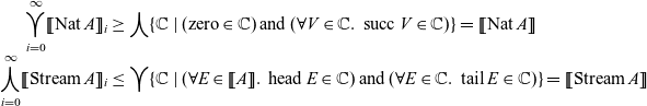
Going the other way, it we need to show that each approximation $[\![ \operatorname{Nat} ]\!]_i$
is a subtype of the
$[\![ \operatorname{Nat} ]\!]_i$
is a subtype of the $\mathbb{C}$
s that make up
$\mathbb{C}$
s that make up $[\![ \operatorname{Nat} ]\!]$
, and dually that each approximation
$[\![ \operatorname{Nat} ]\!]$
, and dually that each approximation $[\![ \operatorname{Stream} A ]\!]_i$
is a supertype of the
$[\![ \operatorname{Stream} A ]\!]_i$
is a supertype of the $\mathbb{C}$
s that make up
$\mathbb{C}$
s that make up $[\![ \operatorname{Stream} A ]\!]$
. Suppose that
$[\![ \operatorname{Stream} A ]\!]$
. Suppose that $\mathbb{C}$
is any reducibility candidate such that
$\mathbb{C}$
is any reducibility candidate such that $N(\mathbb{C}) \leq \mathbb{C}$
. Then
$N(\mathbb{C}) \leq \mathbb{C}$
. Then $[\![ \operatorname{Nat} ]\!]_i \leq \mathbb{C}$
follows by induction on i:
$[\![ \operatorname{Nat} ]\!]_i \leq \mathbb{C}$
follows by induction on i:
(0)
$[\![ \operatorname{Nat} ]\!]_0 = \operatorname{Pos}\{\}$
is the least reducibility candidate w.r.t subtyping, so
$[\![ \operatorname{Nat} ]\!]_0 \leq \mathbb{C}$
.(
$i+1$
) Assume that
$[\![ \operatorname{Nat} ]\!]_i \leq \mathbb{C}$
. The next approximation is
$[\![ \operatorname{Nat} ]\!]_{i+1} = N([\![ \operatorname{Nat} ]\!]_i)$
. Therefore,
\begin{align*} [\![ \operatorname{Nat} ]\!]_{i+1} = N([\![ \operatorname{Nat} ]\!]_i) \leq N(\mathbb{C}) \leq \mathbb{C} \end{align*}
by monotonicity of N (Lemma 1.23).


Similarly, suppose that $\mathbb{C}$
is any reducibility candidate such that
$\mathbb{C}$
is any reducibility candidate such that $S_{[\![ A ]\!]}(\mathbb{C}) \geq \mathbb{C}$
. Then,
$S_{[\![ A ]\!]}(\mathbb{C}) \geq \mathbb{C}$
. Then, $[\![ \operatorname{Stream} A ]\!]_i \geq \mathbb{C}$
follows by induction on i:
$[\![ \operatorname{Stream} A ]\!]_i \geq \mathbb{C}$
follows by induction on i:
(0)
$[\![ \operatorname{Stream} A ]\!]_0 = \operatorname{Neg}\{\}$
is the greatest reducibility candidate w.r.t subtyping, so
$[\![ \operatorname{Stream} A ]\!]_0 \geq \mathbb{C}$
trivially.(
$i+1$
) Assume that
$[\![ \operatorname{Stream} A ]\!]_i \geq \mathbb{C}$
. The next approximation is
$[\![ \operatorname{Stream} A ]\!]_{i+1} = S_{[\![ A ]\!]}([\![ \operatorname{Stream} A ]\!]_i)$
. Therefore,
\begin{align*} [\![ \operatorname{Stream} A ]\!]_{i+1} = S_{[\![ A ]\!]}([\![ \operatorname{Stream} A ]\!]_i) \geq S_{[\![ A ]\!]}(\mathbb{C}) \geq \mathbb{C} \end{align*}
by monotonicity of
$S_{[\![ A ]\!]}$
(Lemma 1.23).


In other words, we know that every $\mathbb{C} \geq N(\mathbb{C})$
is an upper bound of all approximations
$\mathbb{C} \geq N(\mathbb{C})$
is an upper bound of all approximations $[\![ \operatorname{Nat} ]\!]_i$
, and every
$[\![ \operatorname{Nat} ]\!]_i$
, and every $\mathbb{C} \leq S_{[\![ A ]\!]}(\mathbb{C})$
is a lower bound of all approximations
$\mathbb{C} \leq S_{[\![ A ]\!]}(\mathbb{C})$
is a lower bound of all approximations $[\![ \operatorname{Stream} A ]\!]_i$
. So because
$[\![ \operatorname{Stream} A ]\!]_i$
. So because
is the least upper bound and
is the greatest lower bound, we have
In other words,
is a lower bound of the $\mathbb{C}$
s that make up
$\mathbb{C}$
s that make up $[\![ \operatorname{Nat} ]\!]$
and
$[\![ \operatorname{Nat} ]\!]$
and
is an upper bound of the $\mathbb{C}$
s that make up
$\mathbb{C}$
s that make up $[\![ \operatorname{Stream} A ]\!]$
(Lemma 1.16). Again, since
$[\![ \operatorname{Stream} A ]\!]$
(Lemma 1.16). Again, since
is the greatest lower bound and
is the least upper bound, we have
1.5 Adequacy
To conclude, we give the full proof of adequacy (Lemma 6.11) here. With the lemmas that precede in Appendix 1.4, the remaining details are now totally standard. Soundness ensures the safety of the $\mathit{Cut}$
rule and completeness ensures that the terms of each type are included in their interpretations as reducibility candidates. The main role of adequacy is to show that the guarantees given by the premises of each typing rule are strong enough to prove their conclusion and that the notion of substitution corresponds to the interpretation of typing environments.
$\mathit{Cut}$
rule and completeness ensures that the terms of each type are included in their interpretations as reducibility candidates. The main role of adequacy is to show that the guarantees given by the premises of each typing rule are strong enough to prove their conclusion and that the notion of substitution corresponds to the interpretation of typing environments.
Lemma 6.11 (Adequacy).
-
1. If
$\Gamma \vdash c$
is derivable then
$[\![\Gamma \vdash c]\!]$
is true.
-
2. If
$\Gamma \vdash v : A$
is derivable then
$[\![\Gamma \vdash v : A ]\!]$
is true.
-
3. If
$\Gamma \vdash e \div A$
is derivable then
$[\![\Gamma \vdash e \div A ]\!]$
is true.


Proof By (mutual) induction on the given typing derivation for the command or (co)term:
(
$\mathit{Cut}$
) Inductive Hypothesis:
$[\![\Gamma \vdash v : A ]\!]$
and
$[\![\Gamma \vdash e \div A ]\!]$
.Let
$\rho \in [\![ \Gamma ]\!]$
, so
$v[{\rho}]\in[\![ A ]\!]$
and
$e[{\rho}]\in[\![ A ]\!]$
by the inductive hypothesis. Observe that
\begin{align*} \langle {v} |\!| {e} \rangle[{\rho}] = \langle {v[{\rho}]} |\!| {e[{\rho}]} \rangle \in \unicode{x2AEB} \end{align*}
because all reducibility candidates are sound. In other words,
$[\![\Gamma \vdash [\![ {v} |\!| {e} ]\!] \ ]\!]$
.(
$\mathit{VarR}$
and
$\mathit{VarL}$
)
$x[{\rho}] \in [\![ A ]\!]$
for any
$\rho \in [\![\Gamma, x : A]\!]$
by definition. Dually,
$\alpha[{\rho}] \in [\![ A ]\!]$
for any
$\rho \in [\![\Gamma, \alpha \div A]\!]$
by definition. In other words,
$[\![\Gamma, x : A \vdash x : A]\!]$
and
$[\![\Gamma, \alpha \div A \vdash \alpha \div A]\!]$
.(
$\mathit{ActR}$
) Inductive Hypothesis:
$[\![\Gamma, \alpha \div A \vdash c \ ]\!]$
.Let
$\rho \in [\![ \Gamma ]\!]$
, so that for all
$E \in [\![ A ]\!]$
,
${E}/{\alpha},\rho \in [\![\Gamma, \alpha \div A]\!]$
by definition and
\begin{align*} c[{\rho}][{{E}/{\alpha}}] = c[{\rho,{E}/{\alpha}}] \in \unicode{x2AEB} \end{align*}
by the inductive hypothesis. Thus,
\begin{align*} (\mu{\alpha}. c)[{\rho}] = \mu{\alpha}. (c[{\rho}]) \in [\![ A ]\!] \end{align*}
by activation (Lemma 6.3). In other words,
$[\![\Gamma \vdash \mu{\alpha}. c : A]\!]$
.(
$\mathit{ActL}$
) Dual to
$\mathit{ActR}$
above.(
${\to}R$
) Inductive Hypothesis:
$[\![\Gamma, x : A \vdash v : B]\!]$
.Let
$\rho \in [\![ \Gamma ]\!]$
, so for all
$W \in [\![ A ]\!]$
,
${W}/{x},\rho \in [\![\Gamma, x : A]\!]$
by definition and
\begin{align*} v[{\rho}][{{W}/{x}}] = v[{\rho,{W}/{x}}] \in [\![ B ]\!] \end{align*}
by the inductive hypothesis. Thus,
\begin{align*} (\lambda x. v)[{\rho}] = \lambda x. (v[{\rho}]) \in [\![ A \to B ]\!] \end{align*}
Lemma 6.12. In other words
$[\![\Gamma \vdash \lambda x. v : A \to B]\!]$
.(
${\to}L$
) Inductive Hypothesis:
$[\![\Gamma \vdash V : A]\!]$
and
$[\![\Gamma \vdash E \div B]\!]$
.Let
$\rho \in [\![ \Gamma ]\!]$
, so
$V[{\rho}] \in [\![ A ]\!]$
and
$E[{\rho}] \in [\![ B ]\!]$
by the inductive hypothesis. Thus,
\begin{align*} (V \cdot E) [{\rho}] = V[{\rho}] \cdot E[{\rho}] \in [\![ A \to B ]\!] \end{align*}
by definition of
$[\![ A \to B ]\!]$
and Lemma 6.7. In other words,
$[\![\Gamma \vdash V \cdot E \div A \to B]\!]$
.(
${\operatorname{Nat}}R_{\operatorname{zero}}$
): For any substitution
$\rho$
,
\begin{align*} \operatorname{zero}[{\rho}] = \operatorname{zero} \in [\![ \operatorname{Nat} ]\!] \end{align*}
by Lemma 6.7. In other words,
$[\![\Gamma \vdash \operatorname{zero} : \operatorname{Nat}]\!]$
.(
${\operatorname{Nat}}R_{\operatorname{succ}}$
) Inductive Hypothesis:
$[\![\Gamma \vdash V : \operatorname{Nat}]\!]$
.Let
$\rho \in [\![ \Gamma ]\!]$
, so that
$V[{\rho}] \in [\![ \operatorname{Nat} ]\!]$
by the inductive hypothesis. Thus,
\begin{align*} (\operatorname{succ} V)[{\rho}] = \operatorname{succ} (V[{\rho}]) \in [\![ \operatorname{Nat} ]\!] \end{align*}
by Lemma 6.7. In other words,
$[\![\Gamma \vdash \operatorname{succ} V : \operatorname{Nat}]\!]$
.(
${\operatorname{Nat}}L$
) Inductive Hypothesis:
$[\![\Gamma \vdash v : A ]\!]$
,
$[\![\Gamma, x:\operatorname{Nat}, y : A \vdash w : A]\!]$
, and
$[\![ \Gamma \vdash E \div A ]\!]$
.Let
$\rho \in [\![ \Gamma ]\!]$
, so that by the inductive hypothesis:
-
$E[{\rho}] \in [\![ A ]\!]$
,
-
$v [{\rho}] \in [\![ A ]\!]$
, and
-
$w[{\rho}][{{V}/{x},{W}/{y}}] = w[{\rho,{V}/{x},{W}/{y}}] \in [\![ A ]\!]$
for all
$V \in [\![ \operatorname{Nat} ]\!]$
and
$W \in [\![ A ]\!]$
.
Thus,
by Lemmas 6.13 and 1.18. In other words,
\begin{align*} [\![ \Gamma \vdash \operatorname{\mathbf{rec}} \{ \operatorname{zero} \to v \mid \operatorname{succ} x \to y. w \} \operatorname{\mathbf{with}} E \div \operatorname{Nat} ]\!] \end{align*}
(
${\operatorname{Stream}}R$
) Inductive Hypothesis:
$[\![ \Gamma \vdash E \div A ]\!]$
.Let
$\rho \in [\![ \Gamma ]\!]$
, so that
$E[{\rho}] \in [\![ A ]\!]$
by the inductive hypothesis. Thus,
\begin{align*} (\operatorname{head} E)[{\rho}] = \operatorname{head} (E[{\rho}]) \in [\![ \operatorname{Stream} A ]\!] \end{align*}
by Lemma 6.7. In other words,
$[\![\Gamma \vdash \operatorname{head} E \div \operatorname{Stream} A]\!]$
.(
${\operatorname{Stream}}L_{\operatorname{head}}$
) Inductive Hypothesis:
$[\![\Gamma \vdash E \div \operatorname{Stream} A]\!]$
.Let
$\rho \in [\![ \Gamma ]\!]$
, so that
$E[{\rho}] \in [\![ \operatorname{Stream} A ]\!]$
by the inductive hypothesis. Thus,
\begin{align*} (\operatorname{tail} E)[{\rho}] = \operatorname{tail} (E[{\rho}]) \in [\![ \operatorname{Stream} A ]\!] \end{align*}
by Lemma 6.7. In other words,
$[\![\Gamma \vdash \operatorname{tail} E \div \operatorname{Stream} A]\!]$
.(
${\operatorname{Stream}}L_{\operatorname{tail}}$
) Inductive Hypothesis:
$[\![\Gamma, \alpha \div A \vdash e \div B]\!]$
,
$[\![\Gamma, \beta \div \operatorname{Stream} A, \gamma \div B \vdash f \div B]\!]$
, and
$[\![\Gamma \vdash V : B]\!]$
.Let
$\rho \in [\![ \Gamma ]\!]$
, so that by the inductive hypothesis:
–
$V[{\rho}] \in [\![ B ]\!]$
,–
$e[{\rho}][{{E}/{\alpha}}] = e[{\rho,{E}/{\alpha}}] \in [\![ B ]\!]$
for all
$E \in [\![ A ]\!]$
, and–
$f[{\rho}][{{E}/{\beta},{F}/{\gamma}}] = f[{\rho,{E}/{\beta},{F}/{\gamma}}] \in [\![ B ]\!]$
for all
$E \in [\![ \operatorname{Stream} A ]\!]$
and
$F \in [\![ B ]\!]$
.


Thus,

by Lemmas 6.13 and 1.21. In other words
 \begin{equation*} [\![ \Gamma \vdash \operatorname{\mathbf{corec}} \{ \operatorname{head}\alpha \to e \mid \operatorname{tail}\beta \to \gamma. f \} \operatorname{\mathbf{with}} V : \operatorname{Stream} A ]\!] \end{equation*}


 Open access
Discussions
No Discussions have been published for this article.