


1 Introduction
Both the Knuth–Morris–Pratt and the Boyer–Moore algorithms require some complicated preprocessing on the pattern that is difficult to understand and has limited the extent to which they are used.
Robert Sedgewick, Algorithms
String search is a classic problem. Given a string, the pattern, determine if it occurs in a longer string, the text. String search can be solved in  $O(n+m)$ time and O(m) space, where n is the size of the text and m is the size of the pattern. Unfortunately, the algorithm that does so, Knuth–Morris–Pratt (KMP) (Knuth et al., Reference Knuth, Morris and Pratt1977), is hard to understand. Its pseudocode is short, but most explanations of it are not.
Standard treatments, like that of Cormen et al. (Reference Cormen, Leiserson, Rivest and Stein2009) or Sedgewick & Wayne (Reference Sedgewick and Wayne2011), contain headache-inducing descriptions. Actually, neither even explain the genuine KMP algorithm. Cormen et al. explain the simpler Morris–Pratt (MP) algorithm and leave Knuth’s optimization as an exercise. Sedgewick & Wayne present a related algorithm for minimal DFA construction, with greater memory consumption than KMP, and simply assert that it can be improved.
Alternatively, KMP can be derived via program transformation (Takeichi & Akama, Reference Takeichi and Akama1990; Colussi, Reference Colussi1991; Hernández & Rosenblueth, Reference Hernández and Rosenblueth2001; Ager et al., Reference Ager, Danvy and Rohde2003; Bird, Reference Bird2010). Indeed, Knuth himself calculated the algorithm (Knuth et al., Reference Knuth, Morris and Pratt1977, p. 338) from a constructive proof that any language recognizable by a two-way deterministic pushdown automaton can be recognized on a random-access machine in linear time (Cook, Reference Cook1972).
What follows is a journey from naive string search to the full KMP algorithm. Like other derivations, we will take a systematic and incremental approach. Unlike other derivations, visual intuition will be emphasized over program manipulation. The explanation highlights each of the insights that, taken together, lead to an optimal algorithm. Lazy evaluation turns out to be a critical ingredient in the solution.
2 Horizontally naive
The naive O(nm) algorithm for string search attempts to match the pattern at every position in the text. Consider the pattern mama and the text ammamaa. Figure 1 visualizes the naive approach on this example.

Fig. 1. Naive string search (horizontal).
Each row corresponds to a new starting position in the text. Mismatched characters are colored red and underlined. The third row matches fully, indicated by the underlined  $\varepsilon$, so the search is successful. If one just wants to determine if the pattern is present or not, then processing can stop at this point. Related queries, such as counting the number of occurrences of the pattern, require further rows of computation (as shown).
To summarize, naive search finds, if it exists, the left-most suffix of the text whose prefix is the pattern:
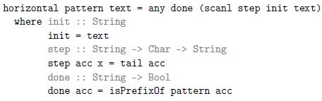
The scanl function is similar to foldl but returns a list of all accumulators instead of just the final one:
The any function determines if some element of the input list satisfies the given predicate:
Coming back to horizontal, the accumulator is initially the entire text. At each step, the accumulator shrinks by one character, generating the next suffix. So, the result of scanl is a list containing all suffixes of the text. Then, any checks to see if some suffix has a prefix that is the pattern.
In the algorithms that follow, any and scanl remain the same; they differ only in the choice of init, step, and done.
3 Vertically naive with a set
Figure 2 is identical to Figure 1 except that it uses vertical lines instead of horizontal ones. This picture suggests a different algorithm. Each column is a set of pattern suffixes, all of which are candidates for a match. Calculating the next column involves three steps:
1. Remove suffixes that do not match the current position in the text (colored red and underlined). These suffixes are failed candidates.
2. Take the tail of those that do. These suffixes remain candidates.
3. Add the pattern itself, corresponding to the diagonal line of mama. Doing so starts a new candidate at each position.

Fig. 2. Naive string search (vertical).
Let us call the result of this procedure the successor of column C on character x. A column containing the empty string, written as  $\varepsilon$, indicates a successful match.
Following this picture yields a new approach. Now, accumulators are columns, columns are sets of strings, and step calculates successors:

As is, verticalSet consumes more memory than horizontal. While step for horizontal does not allocate, step for verticalSet allocates an entirely new set.
There is a trick to negate this drawback. In the same way that sets of natural numbers can be represented using bitstrings, sets of candidate strings can also be represented in binary. Successors can be calculated using left shift and bitwise or. This optimized algorithm, known as Shift-Or (Baeza-Yates & Gonnet, Reference Baeza-Yates and Gonnet1992), performs exceptionally well on small patterns. In particular, Shift-Or works well when the length of the pattern is no greater than the size of a machine word.
Additional notes
String search is equivalent to asking if the regular expression .*pattern.* matches. Compiling this regular expression to an NFA and simulating it shows that the columns of Figure 2 are sets of NFA states. The step function is then the NFA transition function. Equivalently, columns can be viewed as Brzozowski derivatives (Brzozowski, Reference Brzozowski1964; Owens et al., Reference Owens, Reppy and Turon2009) of the regular expression. The step function is then the derivative.
4 Vertically naive with a list
Using a set to represent the accumulator has two drawbacks. First, set operations cannot be fused together. Ideally, step would traverse the accumulator only once, but with sets it must perform more than one traversal. Second, done is not a constant-time operation.
Figure 3 is derived from Figure 2 by removing whitespace from the columns and giving each distinct suffix a unique color and background. This picture suggests representing columns using lists instead of sets, where the first element of the list is the top of the column. The verticalSet function can be easily adapted to this new representation:
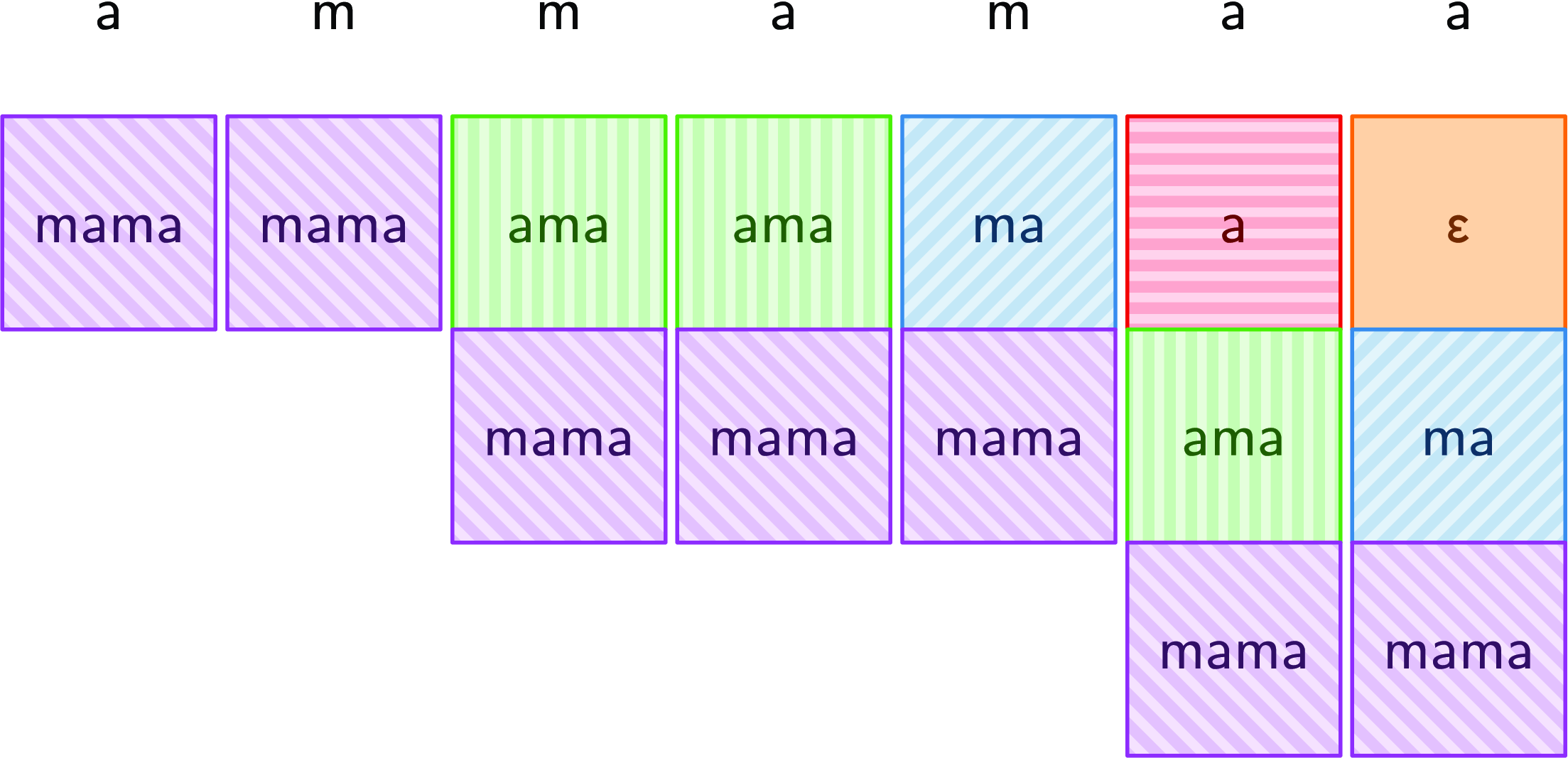
Fig. 3. Columns as lists.
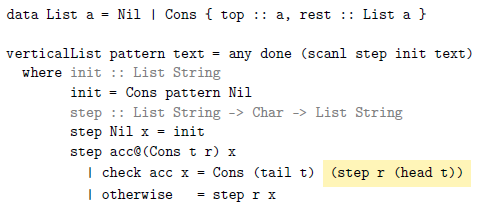
Two features of this snippet may seem unusual now but will be helpful shortly. First, instead of Haskell’s built-in lists, the code defines a new datatype. This will be useful in the next section where this datatype is extended. Second, the highlighted expression could more simply be written as step r x since head t is x in this branch. In the next section, x will be unavailable, and so step r (head t) is the only option at that point.
Now, step is a straightforward recursive function that iterates over the list just once. Moreover, each list is automatically sorted by length. Thus, done can be completed in constant time since it just needs to look at the first element of the list:
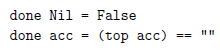
Finally, the check function determines whether the candidate at the top of acc matches the current character of the text:
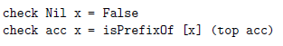
For the remaining algorithms, done and check stay the same.
5 Morris–Pratt
Take another look at Figure 3. There is yet more structure that can be exploited. In particular, two key properties unlock the secret to KMP:
1. For each pattern suffix, there is only one column “shape” where that suffix is top.
2. The rest field of any column is a prior column.
These properties hold for all choices of pattern and text; both can be proved inductively using the definition of step. Informally:
1. To start with, there is only one accumulator: init. A new accumulator can only be generated by calling step acc x when check acc x holds. Doing so yields a new accumulator, where top has shrunk by one character. Additionally, there is only one x such that check acc x holds. Thus, there is only one accumulator of size n, of size $n - 1$, and so forth. Figure 4 shows the five column “shapes” for the pattern mama.
Fig. 4. Column shapes with forward arrows.
2. The rest of column init is empty. All other accumulator values must have been generated by calling step acc x when check acc x holds. Thus, step returns a column where rest is step r (head t). This expression returns a prior column. Figure 5 shows the five columns where rest is indicated by a dashed arrow.
Fig. 5. Column shapes with backward arrows.


Before, we assumed that columns could be any set of pattern suffixes. There are  $2^n$ such sets. Now we know that only n of these sets can ever materialize. Moreover, each column can be represented as a pair consisting of a pattern suffix and a prior column. Combining Figures 4 and 5 yields a compact representation of all possible columns as a graph, pictured in Figure 6.
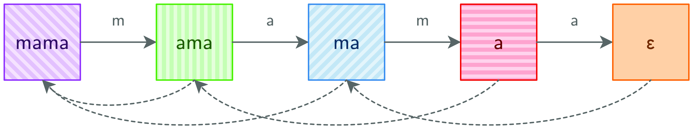
Fig. 6. MP graph.
All that remains is to construct this graph. Just add a next field for the forward edge
and then compute its value with a “smart” constructor (called make here):
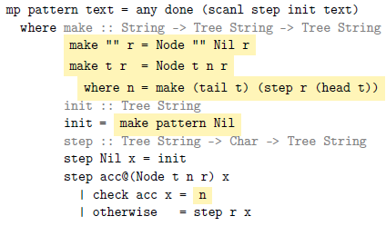
Note how the determination of successor columns has been moved from step (in verticalList) to the constructor (in mp). As a result, init is now the graph from Figure 6. Then, step traverses this graph instead of recomputing successors across the entirety of the text.
In a call-by-value language, this definition would fail because Figure 6 is cyclic. The circularity arises because init is defined in terms of make, which calls step, which returns init in the base case. Fortunately, this kind of cyclic dependency is perfectly acceptable in a lazy language such as Haskell.
This algorithm is called Morris–Pratt (MP), and it runs in linear time. Just a small tweak delivers the full KMP algorithm.
Additional notes
One perspective is that Figure 6 depicts a two-way DFA (Rabin & Scott, Reference Rabin and Scott1959). Backward arrows represent a set of transitions labeled by  $\Sigma \setminus \{x\}$ where x is the matching character. These backward arrows do not consume any input (making it a two-way DFA).
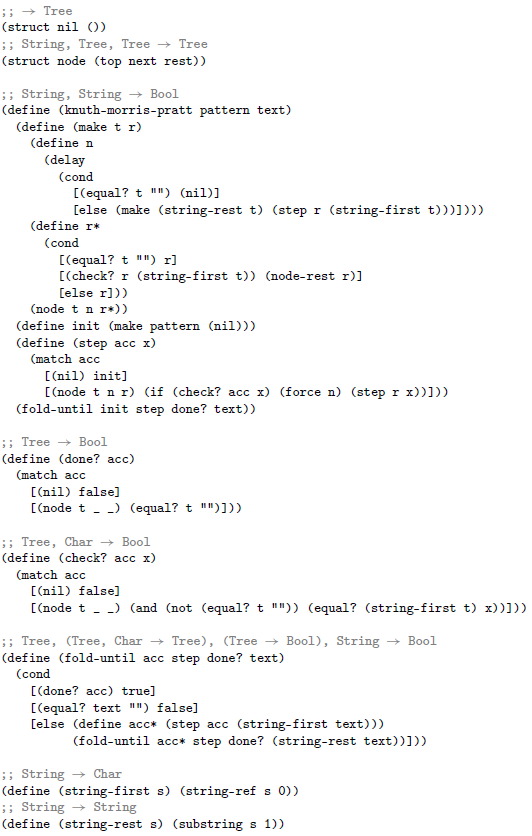
Haskell makes cyclic data construction especially convenient, but it is pretty easy in many eager languages too. Only next needs to be lazy. Appendix A gives a Racket implementation of KMP that uses delay and force to achieve the desired laziness.
Laziness has another benefit. In an eager implementation, the entire graph is always computed, even if it is not needed. In a lazy implementation, if the pattern does not occur in the text, then not of all the graph is used. Thus, not all of the graph is computed.
6 Knuth–Morris–Pratt
Take another look at Figure 6. Suppose the current accumulator is the fourth column (where the top field is a) and the input character is m. That is a mismatch, so MP goes back two columns. That is also a mismatch, so it goes back to the first column. That is a match, so the algorithm ends up at the second column.
Note how a mismatch at column a always skips over column ama because the top values of the two columns start with the same character. Hence, going directly to column mama saves a step. Figure 7 shows the result of transforming Figure 6 according to this insight.
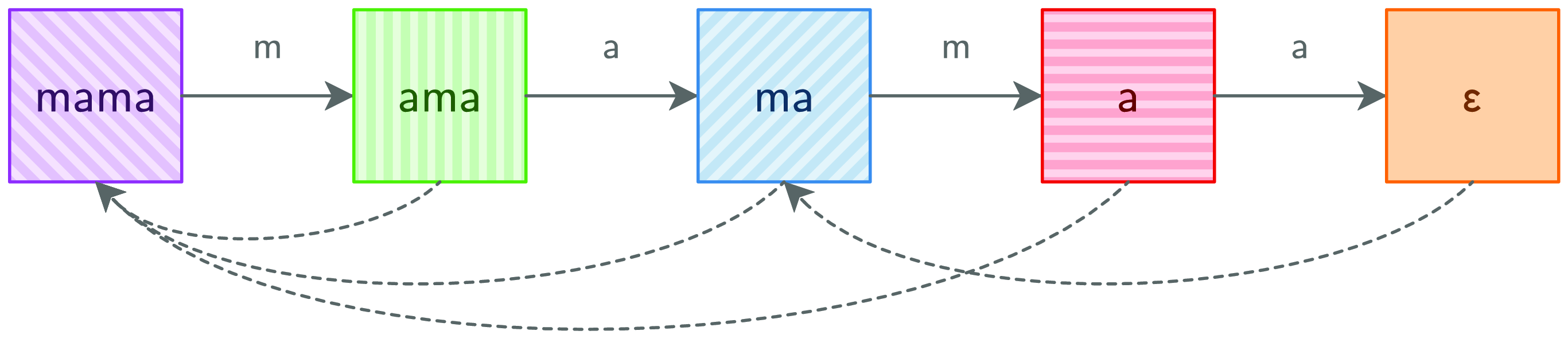
Fig. 7. KMP graph.
Figure 8 shows the code that implements this optimization, delivering the full KMP algorithm. When constructing a column, KMP checks to see if the first character of top matches that of the rest field’s top. If so, it uses the rest field’s rest instead. Since this happens each time a column is constructed, rest is always going to be the “best” column, that is, the earliest one where top has a different first character.
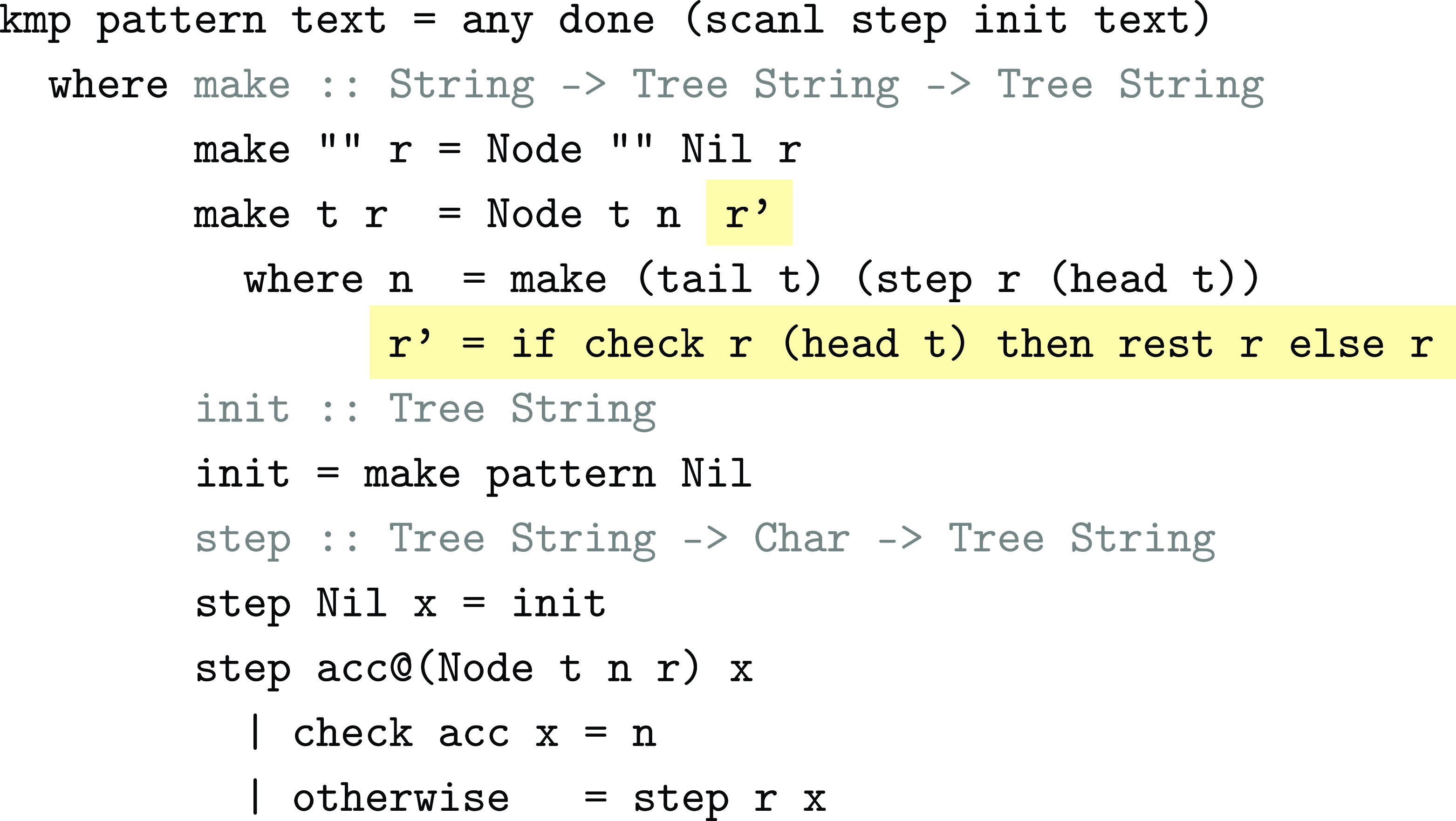
Fig. 8. KMP algorithm.
7 Correctness
One way to test that these implementations are faithful is to check that their traces match a reference implementation (Danvy & Rohde, Reference Danvy and Rohde2006). A trace is the sequence of character comparisons performed during a search. Experiments on a large test suite confirm that the code given in Sections 5 and 6 implement MP and KMP, respectively. Moreover, the number of comparisons made in the KMP implementation is always the same or fewer than in the MP implementation, exactly as expected.
8 Conclusion
Naive string search works row-by-row. Going column-by-column yields a new algorithm, but it is still not linear time. MP takes advantage of the underlying structure of columns, representing them as a cyclic graph. This insight yields a linear-time algorithm. KMP refines this algorithm further, skipping over columns that are guaranteed to fail on a mismatched character.
Acknowledgments
The author thanks Matthias Felleisen, Sam Caldwell, Michael Ballantyne, and anonymous JFP reviewers for their comments and suggestions. This research was supported by National Science Foundation grant SHF 2116372.
Conflicts of Interest
None.
A Racket code


 Open access
Discussions
No Discussions have been published for this article.