


1 Introduction
Reactive systems perform an ongoing interaction with their environment, receiving inputs from the outside, changing their internal state, and producing output. Examples of such systems include GUIs, web applications, video games, and robots. Programming such systems with traditional general-purpose imperative languages can be challenging: the components of the reactive system are put together via a complex and often confusing web of callbacks and shared mutable state. As a consequence, individual components cannot be easily understood in isolation, which makes building and maintaining reactive systems in this manner difficult and error-prone (Parent, Reference Parent2006; Järvi et al., Reference Järvi, Marcus, Parent, Freeman and Smith2008).
Functional reactive programming (FRP), introduced by Elliott and Hudak (Reference Elliott and Hudak1997), tries to remedy this problem by introducing time-varying values (called behaviours or signals) and events as a means of communication between components in a reactive system instead of shared mutable state and callbacks. Crucially, signals and events are first-class values in FRP and can be freely combined and manipulated. These high-level abstractions not only provide a rich and expressive programming model but also make it possible for us to reason about FRP programs by simple equational methods.
Elliott and Hudak’s original conception of FRP is an elegant idea that allows for direct manipulation of time-dependent data but also immediately raises the question of what the interface for signals and events should be. A naive approach would be to model discrete signals as streams defined by the following Haskell data type: Footnote 1
A stream of type $Str\,a$
thus consists of a head of type a and a tail of type
$Str\,a$
thus consists of a head of type a and a tail of type $Str\,a$
. The type
$Str\,a$
. The type $Str\,a$
encodes a discrete signal of type a, where each element of a stream represents the value of that signal at a particular time.
$Str\,a$
encodes a discrete signal of type a, where each element of a stream represents the value of that signal at a particular time.
Combined with the power of higher-order functional programming, we can easily manipulate and compose such signals. For example, we may apply a function to the values of a signal:
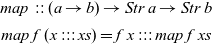 \begin{eqnarray*}
map\, :: (a\to b)\to Str\, a\to Str\, b\nonumber\\
map\, f\,(x ::: xs)=f\,x ::: map\, f\, xs\nonumber
\end{eqnarray*}
\begin{eqnarray*}
map\, :: (a\to b)\to Str\, a\to Str\, b\nonumber\\
map\, f\,(x ::: xs)=f\,x ::: map\, f\, xs\nonumber
\end{eqnarray*}
However, this representation is too permissive and allows the programmer to write non-causal programs, that is, programs where the present output depends on future input such as the following:
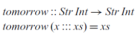
At each time step, this function takes the input of the next time step and returns it in the current time step. In practical terms, this reactive program cannot be effectively executed since we cannot compute the current value of the signal that it defines.
Much of the research in FRP has been dedicated to addressing this problem by adequately restricting the interface that the programmer can use to manipulate signals. This can be achieved by exposing only a carefully selected set of combinators to the programmer or by using a more sophisticated type system. The former approach has been very successful in practice, not least because it can be readily implemented as a library in existing languages. This library approach also immediately integrates the FRP language with a rich ecosystem of existing libraries and inherits the host language’s compiler and tools. The most prominent example of this approach is Arrowised FRP (Nilsson et al., Reference Nilsson, Courtney and Peterson2002), as implemented in the Yampa library for Haskell (Hudak et al., Reference Hudak, Courtney, Nilsson and Peterson2004), which takes signal functions as primitive rather than signals themselves. However, this library approach forfeits some of the simplicity and elegance of the original FRP model as it disallows direct manipulation of signals.
More recently, an alternative to this library approach has been developed (Jeffrey, Reference Jeffrey2014; Krishnaswami and Benton, Reference Krishnaswami and Benton2011; Krishnaswami et al., Reference Krishnaswami, Benton and Hoffmann2012; Krishnaswami Reference Krishnaswami2013; Jeltsch, Reference Jeltsch2013; Bahr et al., Reference Bahr, Graulund and Møgelberg2019, Reference Bahr, Graulund and Møgelberg2021) that uses a modal type operator $\bigcirc$
, which captures the notion of time. Following this idea, an element of type
$\bigcirc$
, which captures the notion of time. Following this idea, an element of type $\bigcirc a$
represents data of type a arriving in the next time step. Signals are then modelled by the type of streams defined instead as follows:
$\bigcirc a$
represents data of type a arriving in the next time step. Signals are then modelled by the type of streams defined instead as follows:
That is, a stream of type $Str\,a$
is an element of type a now and a stream of type
$Str\,a$
is an element of type a now and a stream of type $Str\,a$
later, thus separating consecutive elements of the stream by one time step. Combining this modal type with guarded recursion (Nakano, Reference Nakano2000) in the form of a fixed point operator of type
$Str\,a$
later, thus separating consecutive elements of the stream by one time step. Combining this modal type with guarded recursion (Nakano, Reference Nakano2000) in the form of a fixed point operator of type $(\bigcirc a\to a)\to a$
gives a powerful type system for reactive programming that guarantees not only causality, but also productivity, that is, the property that each element of a stream can be computed in finite time.
$(\bigcirc a\to a)\to a$
gives a powerful type system for reactive programming that guarantees not only causality, but also productivity, that is, the property that each element of a stream can be computed in finite time.
Causality and productivity of an FRP program means that it can be effectively implemented and executed. However, for practical purposes, it is also important whether it can be implemented with given finite resources. If a reactive program requires an increasing amount of memory or computation time, it will eventually run out of resources to make progress or take too long to react to input. It will grind to a halt. Since FRP programs operate on a high level of abstraction, it is typically quite difficult to reason about their space and time cost. A reactive program that exhibits a gradually slower response time, that is, its computations take longer and longer as time progresses, is said to have a time leak. Similarly, we say that a reactive program has a space leak, if its memory use is gradually increasing as time progresses, for example, if it holds on to memory while continually allocating more.
Within both lines of work – the library approach and the modal types approach – there has been an effort to devise FRP languages that avoid implicit space leaks. We say that a space leak is implicit if it is caused not by explicit memory allocations intended by the programmer but rather by the implementation of the FRP language holding on to old data. This is difficult to prevent in a higher-order language as closures may capture references to old data, which consequently must remain in memory for as long as the closure might be invoked. In addition, the language has to carefully balance eager and lazy evaluation: While some computations must necessarily be delayed to wait for input to arrive, we run the risk of needing to keep intermediate values in memory for too long unless we perform computations as soon as all required data have arrived. To avoid implicit space leaks, Ploeg and Claessen (2015) devised an FRP library for Haskell that avoids implicit space leaks by carefully restricting the API to manipulate events and signals. Based on the modal operator $\bigcirc$
described above, Krishnaswami (Reference Krishnaswami2013) has devised a modal FRP calculus that permits an aggressive garbage collection strategy that rules out implicit space leaks.
$\bigcirc$
described above, Krishnaswami (Reference Krishnaswami2013) has devised a modal FRP calculus that permits an aggressive garbage collection strategy that rules out implicit space leaks.
Contributions.
In this paper, we present $\mathsf{Rattus}$
, a practical modal FRP language that takes its ideas from the modal FRP calculi of Krishnaswami (Reference Krishnaswami2013) and Bahr et al. (Reference Bahr, Graulund and Møgelberg2019, Reference Bahr, Graulund and Møgelberg2021) but with a simpler and less restrictive type system that makes it attractive to use in practice. Like the Simply RaTT calculus of Bahr et al., we use a Fitch-style type system (Clouston, Reference Clouston2018), which extends typing contexts with tokens to avoid the syntactic overhead of the dual-context-style type system of Krishnaswami (Reference Krishnaswami2013). In addition, we further simplify the typing system by (1) only requiring one kind of token instead of two, (2) allowing tokens to be introduced without any restrictions, and (3) generalising the guarded recursion scheme. The resulting calculus is simpler and more expressive, yet still retains the operational guarantees of the earlier calculi, namely productivity, causality, and admissibility of an aggressive garbage collection strategy that prevents implicit space leaks. We have proved these properties by a logical relations argument formalised using the Coq theorem prover (see supplementary material and Appendix B).
$\mathsf{Rattus}$
, a practical modal FRP language that takes its ideas from the modal FRP calculi of Krishnaswami (Reference Krishnaswami2013) and Bahr et al. (Reference Bahr, Graulund and Møgelberg2019, Reference Bahr, Graulund and Møgelberg2021) but with a simpler and less restrictive type system that makes it attractive to use in practice. Like the Simply RaTT calculus of Bahr et al., we use a Fitch-style type system (Clouston, Reference Clouston2018), which extends typing contexts with tokens to avoid the syntactic overhead of the dual-context-style type system of Krishnaswami (Reference Krishnaswami2013). In addition, we further simplify the typing system by (1) only requiring one kind of token instead of two, (2) allowing tokens to be introduced without any restrictions, and (3) generalising the guarded recursion scheme. The resulting calculus is simpler and more expressive, yet still retains the operational guarantees of the earlier calculi, namely productivity, causality, and admissibility of an aggressive garbage collection strategy that prevents implicit space leaks. We have proved these properties by a logical relations argument formalised using the Coq theorem prover (see supplementary material and Appendix B).
To demonstrate its use as a practical programming language, we have implemented $\mathsf{Rattus}$
as an embedded language in Haskell. This implementation consists of a library that implements the primitives of the language along with a plugin for the GHC Haskell compiler. The latter is necessary to check the more restrictive variable scope rules of
$\mathsf{Rattus}$
as an embedded language in Haskell. This implementation consists of a library that implements the primitives of the language along with a plugin for the GHC Haskell compiler. The latter is necessary to check the more restrictive variable scope rules of $\mathsf{Rattus}$
and to ensure the eager evaluation strategy that is necessary to obtain the operational properties. Both components are bundled in a single Haskell library that allows the programmer to seamlessly write
$\mathsf{Rattus}$
and to ensure the eager evaluation strategy that is necessary to obtain the operational properties. Both components are bundled in a single Haskell library that allows the programmer to seamlessly write $\mathsf{Rattus}$
code alongside Haskell code. We further demonstrate the usefulness of the language with a number of case studies, including an FRP library based on streams and events as well as an arrowised FRP library in the style of Yampa. We then use both FRP libraries to implement a primitive game. The two libraries implemented in
$\mathsf{Rattus}$
code alongside Haskell code. We further demonstrate the usefulness of the language with a number of case studies, including an FRP library based on streams and events as well as an arrowised FRP library in the style of Yampa. We then use both FRP libraries to implement a primitive game. The two libraries implemented in $\mathsf{Rattus}$
also demonstrate different approaches to FRP libraries: discrete time (streams) versus continuous time (Yampa); and first-class signals (streams) versus signal functions (Yampa). The
$\mathsf{Rattus}$
also demonstrate different approaches to FRP libraries: discrete time (streams) versus continuous time (Yampa); and first-class signals (streams) versus signal functions (Yampa). The $\mathsf{Rattus}$
Haskell library and all examples are included in the supplementary material.
$\mathsf{Rattus}$
Haskell library and all examples are included in the supplementary material.
Overview of paper.
Section 2 gives an overview of the $\mathsf{Rattus}$
language introducing the main concepts and their intuitions. Section 3 presents a case study of a simple FRP library based on streams and events, as well as an arrowised FRP library. Section 4 presents the underlying core calculus of
$\mathsf{Rattus}$
language introducing the main concepts and their intuitions. Section 3 presents a case study of a simple FRP library based on streams and events, as well as an arrowised FRP library. Section 4 presents the underlying core calculus of $\mathsf{Rattus}$
including its type system, its operational semantics, and our main metatheoretical results: productivity, causality, and absence of implicit space leaks. We then reflect on these results and discuss the language design of
$\mathsf{Rattus}$
including its type system, its operational semantics, and our main metatheoretical results: productivity, causality, and absence of implicit space leaks. We then reflect on these results and discuss the language design of $\mathsf{Rattus}$
. Section 5 gives an overview of the proof of our metatheoretical results. Section 6 describes how
$\mathsf{Rattus}$
. Section 5 gives an overview of the proof of our metatheoretical results. Section 6 describes how $\mathsf{Rattus}$
has been implemented as an embedded language in Haskell. Section 7 reviews related work and Section 8 discusses future work.
$\mathsf{Rattus}$
has been implemented as an embedded language in Haskell. Section 7 reviews related work and Section 8 discusses future work.
2 Introduction to Rattus
To illustrate $\mathsf{Rattus}$
, we will use example programs written in the embedding of the language in Haskell. The type of streams is at the centre of these example programs:
$\mathsf{Rattus}$
, we will use example programs written in the embedding of the language in Haskell. The type of streams is at the centre of these example programs:
 \begin{equation*}
\mathbf{data}\; Str\; a =!a:::!(\bigcirc(Str\;a))
\end{equation*}
\begin{equation*}
\mathbf{data}\; Str\; a =!a:::!(\bigcirc(Str\;a))
\end{equation*}
The annotation with bangs (!) ensures that the constructor ::: is strict in both its arguments. We will have a closer look at the evaluation strategy of $\mathsf{Rattus}$
in Section 2.2.
$\mathsf{Rattus}$
in Section 2.2.
The simplest stream one can define just repeats the same value indefinitely. Such a stream is constructed by the $\textit{constInt}$
function below, which takes an integer and produces a constant stream that repeats that integer at every step:
$\textit{constInt}$
function below, which takes an integer and produces a constant stream that repeats that integer at every step:
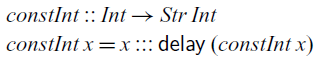
Because the tail of a stream of integers must be of type $\bigcirc(Str\;Int)$
, we have to use
$\bigcirc(Str\;Int)$
, we have to use $\mathsf{delay}$
, which is the introduction form for the type modality
$\mathsf{delay}$
, which is the introduction form for the type modality $\bigcirc$
. Intuitively speaking,
$\bigcirc$
. Intuitively speaking, $\mathsf{delay}$
moves a computation one time step into the future. We could think of
$\mathsf{delay}$
moves a computation one time step into the future. We could think of $\mathsf{delay}$
having type
$\mathsf{delay}$
having type $a\to \bigcirc a$
, but this type is too permissive as it can cause space leaks. It would allow us to move arbitrary computations – and the data they depend on – into the future. Instead, the typing rule for
$a\to \bigcirc a$
, but this type is too permissive as it can cause space leaks. It would allow us to move arbitrary computations – and the data they depend on – into the future. Instead, the typing rule for $\mathsf{delay}$
is formulated as follows:
$\mathsf{delay}$
is formulated as follows:
 \begin{equation*}
\frac{\Gamma,\checkmark\vdash t::A}{\Gamma\vdash\mathsf{delay}\; t::\bigcirc
A}
\end{equation*}
\begin{equation*}
\frac{\Gamma,\checkmark\vdash t::A}{\Gamma\vdash\mathsf{delay}\; t::\bigcirc
A}
\end{equation*}
This is a characteristic example of a Fitch-style typing rule (Clouston, Reference Clouston2018): it introduces the token $\checkmark$
(pronounced ‘tick’) in the typing context
$\checkmark$
(pronounced ‘tick’) in the typing context $\Gamma$
. A typing context consists of type assignments of the form
$\Gamma$
. A typing context consists of type assignments of the form $x::A$
, but it can also contain several occurrences of
$x::A$
, but it can also contain several occurrences of $\checkmark$
. We can think of
$\checkmark$
. We can think of $\checkmark$
as denoting the passage of one time step, that is, all variables to the left of
$\checkmark$
as denoting the passage of one time step, that is, all variables to the left of $\checkmark$
are one time step older than those to the right. In the above typing rule, the term t does not have access to these ‘old’ variables in
$\checkmark$
are one time step older than those to the right. In the above typing rule, the term t does not have access to these ‘old’ variables in $\Gamma$
. There is, however, an exception: if a variable in the typing context is of a type that is time-independent, we still allow t to access them – even if the variable is one time step old. We call these time-independent types stable types, and in particular all base types such as Int and Bool are stable. We will discuss stable types in more detail in Section 2.1.
$\Gamma$
. There is, however, an exception: if a variable in the typing context is of a type that is time-independent, we still allow t to access them – even if the variable is one time step old. We call these time-independent types stable types, and in particular all base types such as Int and Bool are stable. We will discuss stable types in more detail in Section 2.1.
Formally, the variable introduction rule of $\mathsf{Rattus}$
reads as follows:
$\mathsf{Rattus}$
reads as follows:
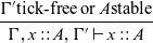 \begin{equation*}
\frac{\Gamma'\text{tick-free}\; \text{or}\; A \text{stable}}{\Gamma,x::A,\Gamma' \vdash x::A}
\end{equation*}
\begin{equation*}
\frac{\Gamma'\text{tick-free}\; \text{or}\; A \text{stable}}{\Gamma,x::A,\Gamma' \vdash x::A}
\end{equation*}
That is, if x is not of a stable type and appears to the left of a $\checkmark$
, then it is no longer in scope.
$\checkmark$
, then it is no longer in scope.
Turning back to our definition of the ${\textit{constInt}}$
function, we can see that the recursive call
${\textit{constInt}}$
function, we can see that the recursive call ${\textit{constInt}\;\textit{x}}$
must be of type
${\textit{constInt}\;\textit{x}}$
must be of type ${\textit{Str}\;\textit{Int}}$
in the context
${\textit{Str}\;\textit{Int}}$
in the context $\Gamma,\checkmark$
, where
$\Gamma,\checkmark$
, where $\Gamma$
contains
$\Gamma$
contains ${\textit{x}\mathbin{::}\textit{Int}}$
. So x remains in scope because it is of type Int, which is a stable type. This would not be the case if we were to generalise
${\textit{x}\mathbin{::}\textit{Int}}$
. So x remains in scope because it is of type Int, which is a stable type. This would not be the case if we were to generalise $\textit{constInt}$
to arbitrary types:
$\textit{constInt}$
to arbitrary types:

In this example, x is of type a and therefore goes out of scope under $\mathsf{delay}$
: since a is not necessarily stable,
$\mathsf{delay}$
: since a is not necessarily stable, $x::a$
is blocked by the
$x::a$
is blocked by the $\checkmark$
introduced by
$\checkmark$
introduced by $\mathsf{delay}$
. We can see that
$\mathsf{delay}$
. We can see that $\textit{leakyConst}$
would indeed cause a space leak by instantiating it to the type
$\textit{leakyConst}$
would indeed cause a space leak by instantiating it to the type $\textit{leakyConst}::\textit{Str}\;\textit{Int}\to \textit{Str}\;(\textit{Str}\;\textit{Int})$
: at each time step n, it would have to store all previously observed input values from time step 0 to
$\textit{leakyConst}::\textit{Str}\;\textit{Int}\to \textit{Str}\;(\textit{Str}\;\textit{Int})$
: at each time step n, it would have to store all previously observed input values from time step 0 to $n- 1$
, thus making its memory usage grow linearly with time. To illustrate this on a concrete example, assume that
$n- 1$
, thus making its memory usage grow linearly with time. To illustrate this on a concrete example, assume that $\textit{leakyConst}$
is fed the stream of numbers
$\textit{leakyConst}$
is fed the stream of numbers $0, 1, 2, \dots$
as input. Then, the resulting stream of type
$0, 1, 2, \dots$
as input. Then, the resulting stream of type $\textit{Str}\;(\textit{Str}\;\textit{Int})$
contains at each time step n the same stream
$\textit{Str}\;(\textit{Str}\;\textit{Int})$
contains at each time step n the same stream $0, 1, 2, \dots$
. However, the input stream arrives one integer at a time. So at time n, the input stream would have advanced to
$0, 1, 2, \dots$
. However, the input stream arrives one integer at a time. So at time n, the input stream would have advanced to $n, n+1, n+2, \dots$
, that is, the next input to arrive is n. Consequently, the implementation of
$n, n+1, n+2, \dots$
, that is, the next input to arrive is n. Consequently, the implementation of $\textit{leakyConst}$
would need to have stored the previous values
$\textit{leakyConst}$
would need to have stored the previous values $0,1, \dots n-1$
of the input stream.
$0,1, \dots n-1$
of the input stream.
The definition of constInt also illustrates the guarded recursion principle used in $\mathsf{Rattus}$
. For a recursive definition to be well-typed, all recursive calls have to occur in the presence of a
$\mathsf{Rattus}$
. For a recursive definition to be well-typed, all recursive calls have to occur in the presence of a $\checkmark$
– in other words, recursive calls have to be guarded by
$\checkmark$
– in other words, recursive calls have to be guarded by $\mathsf{delay}$
. This restriction ensures that all recursive functions are productive, which means that each element of a stream can be computed in finite time. If we did not have this restriction, we could write the following obviously unproductive function:
$\mathsf{delay}$
. This restriction ensures that all recursive functions are productive, which means that each element of a stream can be computed in finite time. If we did not have this restriction, we could write the following obviously unproductive function:

The recursive call to $\textit{loop}$
does not occur under a delay and is thus rejected by the type checker.
$\textit{loop}$
does not occur under a delay and is thus rejected by the type checker.
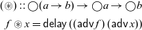
Let’s consider an example program that transforms streams. The function $\textit{inc}$
below takes a stream of integers as input and increments each integer by 1:
$\textit{inc}$
below takes a stream of integers as input and increments each integer by 1:
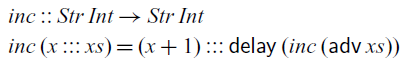
Here we have to use ![]() , the elimination form for
, the elimination form for $\bigcirc$
, to convert the tail of the input stream from type
$\bigcirc$
, to convert the tail of the input stream from type $\bigcirc(Str\;Int)$
into type
$\bigcirc(Str\;Int)$
into type ${\textit{Str}\;\textit{Int}}$
. Again we could think of
${\textit{Str}\;\textit{Int}}$
. Again we could think of ![]() having type
having type $\bigcirc a\to a$
, but this general type would allow us to write non-causal functions such as the
$\bigcirc a\to a$
, but this general type would allow us to write non-causal functions such as the $\textit{tomorrow}$
function we have seen in the introduction:
$\textit{tomorrow}$
function we have seen in the introduction:
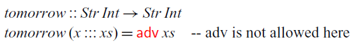
This function looks one time step ahead so that the output at time n depends on the input at time $n+1$
.
$n+1$
.
To ensure causality, ![]() is restricted to contexts with a
is restricted to contexts with a $\checkmark$
:
$\checkmark$
:
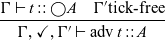 \begin{equation*}
\frac{\Gamma \vdash t::\bigcirc A \quad \Gamma'\text{tick-free}}{\Gamma,\checkmark,\Gamma' \vdash {\rm adv}\; t:: A}
\end{equation*}
\begin{equation*}
\frac{\Gamma \vdash t::\bigcirc A \quad \Gamma'\text{tick-free}}{\Gamma,\checkmark,\Gamma' \vdash {\rm adv}\; t:: A}
\end{equation*}
Not only does ![]() require a
require a $\checkmark$
, but it also causes all bound variables to the right of
$\checkmark$
, but it also causes all bound variables to the right of $\checkmark$
to go out of scope. Intuitively speaking
$\checkmark$
to go out of scope. Intuitively speaking $\mathsf{delay}$
looks ahead one time step and
$\mathsf{delay}$
looks ahead one time step and ![]() then allows us to go back to the present. Variable bindings made in the future are therefore not accessible once we returned to the present.
then allows us to go back to the present. Variable bindings made in the future are therefore not accessible once we returned to the present.
Note that $\mathsf{adv}$
causes the variables to the right of
$\mathsf{adv}$
causes the variables to the right of $\checkmark$
to go out of scope forever, whereas it brings variables back into scope that were previously blocked by the
$\checkmark$
to go out of scope forever, whereas it brings variables back into scope that were previously blocked by the $\checkmark$
. That is, variables that go out of scope due to
$\checkmark$
. That is, variables that go out of scope due to $\mathsf{delay}$
can be brought back into scope by
$\mathsf{delay}$
can be brought back into scope by $\mathsf{adv}$
.
$\mathsf{adv}$
.
2.1 Stable types
We haven’t yet made precise what stable types are. To a first approximation, types are stable if they do not contain $\bigcirc$
or function types. Intuitively speaking,
$\bigcirc$
or function types. Intuitively speaking, $\bigcirc$
expresses a temporal aspect and thus types containing
$\bigcirc$
expresses a temporal aspect and thus types containing $\bigcirc$
are not time-invariant. Moreover, functions can implicitly have temporal values in their closure and are therefore also excluded from stable types.
$\bigcirc$
are not time-invariant. Moreover, functions can implicitly have temporal values in their closure and are therefore also excluded from stable types.
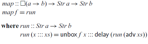
However, as a consequence, we cannot implement the $\textit{map}$
function that takes a function
$\textit{map}$
function that takes a function $f::a\to b$
and applies it to each element of a stream of type
$f::a\to b$
and applies it to each element of a stream of type $Str\,a$
, because it would require us to apply the function f at any time in the future. We cannot do this because
$Str\,a$
, because it would require us to apply the function f at any time in the future. We cannot do this because $a\to b$
is not a stable type (even if a and b were stable) and therefore f cannot be transported into the future. However,
$a\to b$
is not a stable type (even if a and b were stable) and therefore f cannot be transported into the future. However, $\mathsf{Rattus}$
has the type modality
$\mathsf{Rattus}$
has the type modality $\square$
, pronounced ‘box’, that turns any type A into a stable type
$\square$
, pronounced ‘box’, that turns any type A into a stable type $\square A$
. Using the
$\square A$
. Using the $\square$
modality, we can implement
$\square$
modality, we can implement $\textit{map}$
as follows:
$\textit{map}$
as follows:
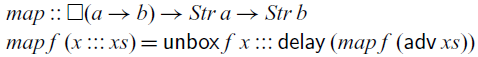
Instead of a function of type $a\to b$
,
$a\to b$
, $\textit{map}$
takes a boxed function f of type
$\textit{map}$
takes a boxed function f of type $\square(a\to b)$
as its argument. That means, f is still in scope under the delay because it is of a stable type. To use f, it has to be unboxed using
$\square(a\to b)$
as its argument. That means, f is still in scope under the delay because it is of a stable type. To use f, it has to be unboxed using $\mathsf{unbox}$
, which is the elimination form for the
$\mathsf{unbox}$
, which is the elimination form for the $\square$
modality and simply has type
$\square$
modality and simply has type $\square a \to a$
, without any restrictions.
$\square a \to a$
, without any restrictions.
The corresponding introduction form for $\square$
does come with some restrictions. It has to make sure that boxed values only refer to variables of a stable type:
$\square$
does come with some restrictions. It has to make sure that boxed values only refer to variables of a stable type:
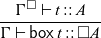 \begin{equation*}
\frac{\Gamma^{\square} \vdash t:: A}
{\Gamma \vdash \mathsf{box}\;t::\square A}
\end{equation*}
\begin{equation*}
\frac{\Gamma^{\square} \vdash t:: A}
{\Gamma \vdash \mathsf{box}\;t::\square A}
\end{equation*}
Here, $\Gamma^{\square}$
denotes the typing context that is obtained from
$\Gamma^{\square}$
denotes the typing context that is obtained from $\Gamma$
by removing all variables of non-stable types and all
$\Gamma$
by removing all variables of non-stable types and all $\checkmark$
tokens:
$\checkmark$
tokens:
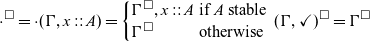 \begin{equation*}
\cdot^{\square} = \cdot
(\Gamma,x::A) = \left\{
\begin{array}{@{}lll@{}}
\Gamma^{\square},x::A & \text{if } A \text{ stable}\\
\Gamma^{\square}& \text{otherwise}
\end{array}\right.
(\Gamma,\checkmark)^{\square} =\Gamma^{\square}
\end{equation*}
\begin{equation*}
\cdot^{\square} = \cdot
(\Gamma,x::A) = \left\{
\begin{array}{@{}lll@{}}
\Gamma^{\square},x::A & \text{if } A \text{ stable}\\
\Gamma^{\square}& \text{otherwise}
\end{array}\right.
(\Gamma,\checkmark)^{\square} =\Gamma^{\square}
\end{equation*}
Thus, for a well-typed term $\mathsf{box}\;t$
, we know that t only accesses variables of stable type.
$\mathsf{box}\;t$
, we know that t only accesses variables of stable type.
For example, we can implement the $\textit{inc}$
function using
$\textit{inc}$
function using $\textit{map}$
as follows:
$\textit{map}$
as follows:
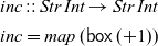 \begin{align*}
\textit{inc}::\textit{Str}\;\textit{Int}\to \textit{Str}\;\textit{Int}\\
\textit{inc}=\textit{map}\;(\mathsf{box}\;(+1))
\end{align*}
\begin{align*}
\textit{inc}::\textit{Str}\;\textit{Int}\to \textit{Str}\;\textit{Int}\\
\textit{inc}=\textit{map}\;(\mathsf{box}\;(+1))
\end{align*}
Using the $\square$
modality, we can also generalise the constant stream function to arbitrary boxed types:
$\square$
modality, we can also generalise the constant stream function to arbitrary boxed types:
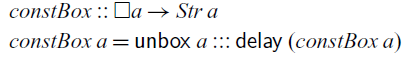
Alternatively, we can make use of the $\textit{Stable}$
type class, to constrain type variables to stable types:
$\textit{Stable}$
type class, to constrain type variables to stable types:
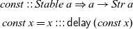 \begin{align*}
\textit{const}::\textit{Stable}\;a\Rightarrow a\to \textit{Str}\;a\\
\textit{const}\;x=x:::\mathsf{delay}\;(\textit{const}\;x)
\end{align*}
\begin{align*}
\textit{const}::\textit{Stable}\;a\Rightarrow a\to \textit{Str}\;a\\
\textit{const}\;x=x:::\mathsf{delay}\;(\textit{const}\;x)
\end{align*}
Since the type of streams is not stable, the restriction to stable types disallows the instantiation of the $\textit{const}$
function to the type
$\textit{const}$
function to the type $\textit{Str}\;\textit{Int}\to \textit{Str}\;(\textit{Str}\;\textit{Int})$
, which as we have seen earlier would cause a memory leak. By contrast,
$\textit{Str}\;\textit{Int}\to \textit{Str}\;(\textit{Str}\;\textit{Int})$
, which as we have seen earlier would cause a memory leak. By contrast, $\textit{constBox}$
can be instantiated to the type
$\textit{constBox}$
can be instantiated to the type $\square(\textit{Str}\;\textit{Int})\to \textit{Str}\;(\textit{Str}\;\textit{Int})$
. This is unproblematic since a value of type
$\square(\textit{Str}\;\textit{Int})\to \textit{Str}\;(\textit{Str}\;\textit{Int})$
. This is unproblematic since a value of type $\square(\textit{Str}\;\textit{Int})$
is a suspended, time-invariant computation that produces an integer stream. In other words, this computation is independent of any external input and can thus be executed at any time in the future without keeping old temporal values in memory.
$\square(\textit{Str}\;\textit{Int})$
is a suspended, time-invariant computation that produces an integer stream. In other words, this computation is independent of any external input and can thus be executed at any time in the future without keeping old temporal values in memory.
So far, we have only looked at recursive definitions at the top level. Recursive definitions can also be nested, but we have to be careful how such nested recursion interacts with the typing environment. Below is an alternative definition of $\textit{map}$
that takes the boxed function f as an argument and then calls the
$\textit{map}$
that takes the boxed function f as an argument and then calls the $\textit{run}$
function that recurses over the stream:
$\textit{run}$
function that recurses over the stream:
Here, $\textit{run}$
is type-checked in a typing environment
$\textit{run}$
is type-checked in a typing environment $\Gamma$
that contains
$\Gamma$
that contains $f::\square(a\to b)$
. Since
$f::\square(a\to b)$
. Since $\textit{run}$
is defined by guarded recursion, we require that its definition must type-check in the typing context
$\textit{run}$
is defined by guarded recursion, we require that its definition must type-check in the typing context $\Gamma^{\square}$
. Because f is of a stable type, it remains in
$\Gamma^{\square}$
. Because f is of a stable type, it remains in $\Gamma^{\square}$
and is thus in scope in the definition of
$\Gamma^{\square}$
and is thus in scope in the definition of $\textit{run}$
. That is, guarded recursive definitions interact with the typing environment in the same way as
$\textit{run}$
. That is, guarded recursive definitions interact with the typing environment in the same way as $\mathsf{box}$
, which ensures that such recursive definitions are stable and can thus safely be executed at any time in the future. As a consequence, the type checker will prevent us from writing the following leaky version of
$\mathsf{box}$
, which ensures that such recursive definitions are stable and can thus safely be executed at any time in the future. As a consequence, the type checker will prevent us from writing the following leaky version of $\textit{map}$
:
$\textit{map}$
:
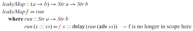
The type of f is not stable, and thus it is not in scope in the definition of $\textit{run}$
.
$\textit{run}$
.
Note that top-level defined identifiers such as $\textit{map}$
and
$\textit{map}$
and $\textit{const}$
are in scope in any context after they are defined regardless of whether there is a
$\textit{const}$
are in scope in any context after they are defined regardless of whether there is a $\checkmark$
or whether they are of a stable type. One can think of top-level definitions being implicitly boxed when they are defined and implicitly unboxed when they are used later on.
$\checkmark$
or whether they are of a stable type. One can think of top-level definitions being implicitly boxed when they are defined and implicitly unboxed when they are used later on.
2.2 Operational semantics
As we have seen in the examples above, the purpose of the type modalities $\bigcirc$
and
$\bigcirc$
and $\square$
is to ensure that
$\square$
is to ensure that $\mathsf{Rattus}$
programs are causal, productive and without implicit space leaks. In simple terms, the latter means that temporal values, that is, values of type
$\mathsf{Rattus}$
programs are causal, productive and without implicit space leaks. In simple terms, the latter means that temporal values, that is, values of type $\bigcirc{A}$
, are safe to be garbage collected after two time steps. In particular, input from a stream can be safely garbage collected one time step after it has arrived. This memory property is made precise later in Section 4 along with a precise definition of the operational semantics of
$\bigcirc{A}$
, are safe to be garbage collected after two time steps. In particular, input from a stream can be safely garbage collected one time step after it has arrived. This memory property is made precise later in Section 4 along with a precise definition of the operational semantics of $\mathsf{Rattus}$
.
$\mathsf{Rattus}$
.
To obtain this memory property, $\mathsf{Rattus}$
uses an eager evaluation strategy except for
$\mathsf{Rattus}$
uses an eager evaluation strategy except for $\mathsf{delay}$
and
$\mathsf{delay}$
and $\mathsf{box}$
. That is, arguments are evaluated to values before they are passed on to functions, but special rules apply to
$\mathsf{box}$
. That is, arguments are evaluated to values before they are passed on to functions, but special rules apply to $\mathsf{delay}$
and
$\mathsf{delay}$
and $\mathsf{box}$
. In addition, we only allow strict data types in
$\mathsf{box}$
. In addition, we only allow strict data types in $\mathsf{Rattus}$
, which explains the use of strictness annotations in the definition of
$\mathsf{Rattus}$
, which explains the use of strictness annotations in the definition of $\textit{Str}$
. This eager evaluation strategy ensures that we do not have to keep intermediate values in memory for longer than one time step.
$\textit{Str}$
. This eager evaluation strategy ensures that we do not have to keep intermediate values in memory for longer than one time step.
Following the temporal interpretation of the $\bigcirc$
modality, its introduction form
$\bigcirc$
modality, its introduction form $\mathsf{delay}$
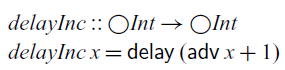
does not eagerly evaluate its argument since we may have to wait until input data arrives. For example, in the following function, we cannot evaluate
$\mathsf{delay}$
does not eagerly evaluate its argument since we may have to wait until input data arrives. For example, in the following function, we cannot evaluate ${\rm adv}\;x+1$
until the integer value of
${\rm adv}\;x+1$
until the integer value of $x::\bigcirc\textit{Int}$
arrives, which is one time step from now:
$x::\bigcirc\textit{Int}$
arrives, which is one time step from now:
However, evaluation is only delayed by one time step, and this delay is reversed by adv. For example, ${\rm adv}\;(\mathsf{delay}\;(1+1))$
evaluates immediately to 2.
${\rm adv}\;(\mathsf{delay}\;(1+1))$
evaluates immediately to 2.
Turning to $\mathsf{box}$
, we can see that it needs to lazily evaluate its argument in order to maintain the memory property of
$\mathsf{box}$
, we can see that it needs to lazily evaluate its argument in order to maintain the memory property of $\mathsf{Rattus}$
: in the expression
$\mathsf{Rattus}$
: in the expression $\mathsf{box}\;(\mathsf{delay}\;1)$
of type
$\mathsf{box}\;(\mathsf{delay}\;1)$
of type $\square(\bigcirc\textit{Int})$
, we should not evaluate
$\square(\bigcirc\textit{Int})$
, we should not evaluate ${\mathsf{delay}\;1}$
right away. As mention above, values of type
${\mathsf{delay}\;1}$
right away. As mention above, values of type ${\bigcirc\textit{Int}}$
should be garbage collected after two time steps. However, boxed types are stable and can thus be moved arbitrarily into the future. Hence, by the time this boxed value is unboxed in the future, we might have already garbage collected the value of type
${\bigcirc\textit{Int}}$
should be garbage collected after two time steps. However, boxed types are stable and can thus be moved arbitrarily into the future. Hence, by the time this boxed value is unboxed in the future, we might have already garbage collected the value of type ${\bigcirc\textit{Int}}$
it contains.
${\bigcirc\textit{Int}}$
it contains.
The modal FRP calculi of Krishnaswami (Reference Krishnaswami2013) and Bahr et al. (Reference Bahr, Graulund and Møgelberg2019, Reference Bahr, Graulund and Møgelberg2021) have a similar operational semantics to achieve same memory property that $\mathsf{Rattus}$
has. However,
$\mathsf{Rattus}$
has. However, $\mathsf{Rattus}$
uses a slightly more eager evaluation strategy for
$\mathsf{Rattus}$
uses a slightly more eager evaluation strategy for $\mathsf{delay}$
: recall that
$\mathsf{delay}$
: recall that $\mathsf{delay}\,t$
delays the computation t by one time step and that
$\mathsf{delay}\,t$
delays the computation t by one time step and that $\mathsf{adv}$
reverses such a delay. The operational semantics of
$\mathsf{adv}$
reverses such a delay. The operational semantics of $\mathsf{Rattus}$
reflects this intuition by first evaluating every term t that occurs as
$\mathsf{Rattus}$
reflects this intuition by first evaluating every term t that occurs as $\mathsf{delay}\,(\dots \mathsf{adv}\,t \dots)$
before evaluating
$\mathsf{delay}\,(\dots \mathsf{adv}\,t \dots)$
before evaluating $\mathsf{delay}$
. In other words,
$\mathsf{delay}$
. In other words, $\mathsf{delay}\,(\dots \mathsf{adv}\,t \dots)$
is equivalent to
$\mathsf{delay}\,(\dots \mathsf{adv}\,t \dots)$
is equivalent to
 \begin{equation*}
\mathsf{let} x t {\mathsf{delay}\,(\dots \mathsf{adv}\,x \dots)}
\end{equation*}
\begin{equation*}
\mathsf{let} x t {\mathsf{delay}\,(\dots \mathsf{adv}\,x \dots)}
\end{equation*}
This adjustment of the operational semantics of $\mathsf{delay}$
is important, as it allows us to lift the restrictions present in previous calculi (Krishnaswami Reference Krishnaswami2013; Bahr et al., Reference Bahr, Graulund and Møgelberg2019, Reference Bahr, Graulund and Møgelberg2021) that disallow guarded recursive definitions to ‘look ahead’ more than one time step. In the Fitch-style calculi of Bahr et al. (Reference Bahr, Graulund and Møgelberg2019, Reference Bahr, Graulund and Møgelberg2021), this can be seen in the restriction to allow at most one
$\mathsf{delay}$
is important, as it allows us to lift the restrictions present in previous calculi (Krishnaswami Reference Krishnaswami2013; Bahr et al., Reference Bahr, Graulund and Møgelberg2019, Reference Bahr, Graulund and Møgelberg2021) that disallow guarded recursive definitions to ‘look ahead’ more than one time step. In the Fitch-style calculi of Bahr et al. (Reference Bahr, Graulund and Møgelberg2019, Reference Bahr, Graulund and Møgelberg2021), this can be seen in the restriction to allow at most one $\checkmark$
in the typing context. For the same reason, these two calculi also disallow function definitions in the context of a
$\checkmark$
in the typing context. For the same reason, these two calculi also disallow function definitions in the context of a $\checkmark$
. As a consequence, terms like
$\checkmark$
. As a consequence, terms like $\mathsf{delay}(\mathsf{delay}\, 0)$
and
$\mathsf{delay}(\mathsf{delay}\, 0)$
and $\mathsf{delay}(\lambda x. x)$
do not type-check in the calculi of Bahr et al. (Reference Bahr, Graulund and Møgelberg2019); Bahr et al. (Reference Bahr, Graulund and Møgelberg2021).
$\mathsf{delay}(\lambda x. x)$
do not type-check in the calculi of Bahr et al. (Reference Bahr, Graulund and Møgelberg2019); Bahr et al. (Reference Bahr, Graulund and Møgelberg2021).
The extension in expressive power afforded by $\mathsf{Rattus}$
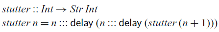
’s slightly more eager evaluation strategy has immediate practical benefits: most importantly, there are no restrictions on where one can define functions. Secondly, we can write recursive functions that look several steps into the future:
$\mathsf{Rattus}$
’s slightly more eager evaluation strategy has immediate practical benefits: most importantly, there are no restrictions on where one can define functions. Secondly, we can write recursive functions that look several steps into the future:
Applying $\textit{stutter}$
to 0 would construct a stream of numbers
$\textit{stutter}$
to 0 would construct a stream of numbers $0, 0, 1, 1, 2, 2, \ldots$
. In order to implement
$0, 0, 1, 1, 2, 2, \ldots$
. In order to implement $\textit{stutter}$
in the more restrictive language of Krishnaswami (Reference Krishnaswami2013) and Bahr et al. (Reference Bahr, Graulund and Møgelberg2019, Reference Bahr, Graulund and Møgelberg2021), we would need to decompose it into two mutually recursive functions (Bahr et al., Reference Bahr, Graulund and Møgelberg2021). A more detailed comparison of the expressive power of these calculi can be found in Section 4.5
$\textit{stutter}$
in the more restrictive language of Krishnaswami (Reference Krishnaswami2013) and Bahr et al. (Reference Bahr, Graulund and Møgelberg2019, Reference Bahr, Graulund and Møgelberg2021), we would need to decompose it into two mutually recursive functions (Bahr et al., Reference Bahr, Graulund and Møgelberg2021). A more detailed comparison of the expressive power of these calculi can be found in Section 4.5
At first glance, one might think that allowing multiple ticks could be accommodated without changing the evaluation of $\mathsf{delay}$
and instead extending the time one has to keep temporal values in memory accordingly, that is, we may safely garbage collect temporal values after
$\mathsf{delay}$
and instead extending the time one has to keep temporal values in memory accordingly, that is, we may safely garbage collect temporal values after $n+1$
time steps, if we allow at most n ticks. However, as we will demonstrate in Section 4.3.3, this is not enough. Even allowing just two ticks would require us to keep temporal values in memory indefinitely, that is, it would permit implicit space leaks. On the other hand, given the more eager evaluation strategy for
$n+1$
time steps, if we allow at most n ticks. However, as we will demonstrate in Section 4.3.3, this is not enough. Even allowing just two ticks would require us to keep temporal values in memory indefinitely, that is, it would permit implicit space leaks. On the other hand, given the more eager evaluation strategy for $\mathsf{delay}$
, we can still garbage collect all temporal values after two time steps, no matter how many ticks were involved in type-checking the program.
$\mathsf{delay}$
, we can still garbage collect all temporal values after two time steps, no matter how many ticks were involved in type-checking the program.
3 Reactive programming in Rattus
In this section, we showcase how
 \begin{equation*}\mathsf{Rattus}\end{equation*}
can be used for reactive programming. To this end, we implement a small library of combinators for programming with streams and events. We then use this library to implement a simple game. Finally, we implement a Yampa-style library and re-implement the game using that library instead. The full sources of both implementations of the game are included in the supplementary material along with a third variant that uses a combinator library based on monadic streams (Perez et al., Reference Perez, Bärenz and Nilsson2016).
3.1 Programming with streams and events
To illustrate how
 \begin{equation*}\mathsf{Rattus}\end{equation*}
facilitates working with streams and events, we have implemented a small set of combinators, as shown in Figure 1. The $\textit{map}$
function should be familiar by now. The
$\textit{map}$
function should be familiar by now. The $\textit{zip}$
function combines two streams similarly to Haskell’s
$\textit{zip}$
function combines two streams similarly to Haskell’s $\textit{zip}$
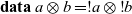
function defined on lists. Note however that instead of the normal pair type, we use a strict pair type:
$\textit{zip}$
function defined on lists. Note however that instead of the normal pair type, we use a strict pair type:
 \begin{equation*}
\mathbf{data}\;a\otimes b= ! a\otimes\mathbin{!} b
\end{equation*}
\begin{equation*}
\mathbf{data}\;a\otimes b= ! a\otimes\mathbin{!} b
\end{equation*}
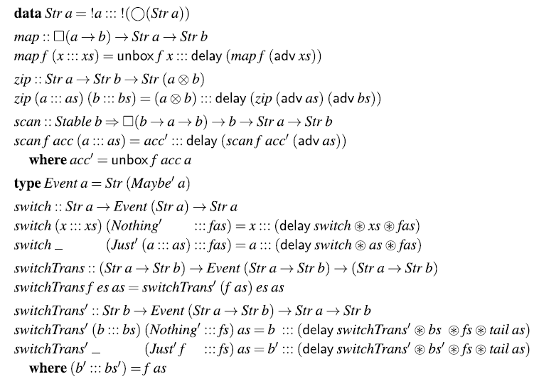
Fig. 1. Small library for streams and events.
It is like the normal pair type (a,b), but when constructing a strict pair ${s\otimes t}$
, the two components s and t are evaluated to weak head normal form.
${s\otimes t}$
, the two components s and t are evaluated to weak head normal form.
The $\textit{scan}$
function is similar to Haskell’s
$\textit{scan}$
function is similar to Haskell’s $\textit{scanl}$
function on lists: given a stream of values
$\textit{scanl}$
function on lists: given a stream of values $\textit{v}_{{\rm 0}},v_{1},v_{2},\ldots$
, the expression
$\textit{v}_{{\rm 0}},v_{1},v_{2},\ldots$
, the expression $\textit{scan}\;(\mathsf{box}\;f)\;{v}$
computes the stream
$\textit{scan}\;(\mathsf{box}\;f)\;{v}$
computes the stream
 \begin{equation*}
f\;\textit{v}\;\textit{v}_{\mathrm{0}},\quad
{f\;(f\;\textit{v}\;\textit{v}_{\mathrm{0}})\;\textit{v}_{1},}\quad {f\;(f\;(f\;\textit{v}\;\textit{v}_{\mathrm{0}})\;\textit{v}_{1})\;\textit{v}_{\mathrm{2}},}\quad\ldots
\end{equation*}
\begin{equation*}
f\;\textit{v}\;\textit{v}_{\mathrm{0}},\quad
{f\;(f\;\textit{v}\;\textit{v}_{\mathrm{0}})\;\textit{v}_{1},}\quad {f\;(f\;(f\;\textit{v}\;\textit{v}_{\mathrm{0}})\;\textit{v}_{1})\;\textit{v}_{\mathrm{2}},}\quad\ldots
\end{equation*}
If one would want a variant of $\textit{scan}$
that is closer to Haskell’s
$\textit{scan}$
that is closer to Haskell’s $\textit{scanl}$
, that is, the result starts with the value v instead of
$\textit{scanl}$
, that is, the result starts with the value v instead of ${f\;v\;v_{0}}$
, one can simply replace the first occurrence of
${f\;v\;v_{0}}$
, one can simply replace the first occurrence of $\textit{acc}'$
in the definition of
$\textit{acc}'$
in the definition of $\textit{scan}$
with
$\textit{scan}$
with $\textit{acc}$
. Note that the type b has to be stable in the definition of
$\textit{acc}$
. Note that the type b has to be stable in the definition of $\textit{scan}$
so that
$\textit{scan}$
so that $\textit{acc}'::b$
is still in scope under
$\textit{acc}'::b$
is still in scope under $\mathsf{delay}$
.
$\mathsf{delay}$
.
A central component of FRP is that it must provide a way to react to events. In particular, it must support the ability to switch behaviour in response to the occurrence of an event. There are different ways to represent events. The simplest representation defines events of type a as streams of type $\textit{Maybe}\;a$
. However, we will use the strict variant of the
$\textit{Maybe}\;a$
. However, we will use the strict variant of the ${\textit{Maybe}}$
type:
${\textit{Maybe}}$
type:
 \begin{equation*}
\mathbf{data}\;\textit{Maybe}'\;a=\textit{Just}'{!}\! a\mid
\textit{Nothing}'
\end{equation*}
\begin{equation*}
\mathbf{data}\;\textit{Maybe}'\;a=\textit{Just}'{!}\! a\mid
\textit{Nothing}'
\end{equation*}
We can then devise a simple ${\textit{switch}}$
combinator that reacts to events. Given an initial stream xs and an event e that may produce a stream, swith xs e initially behaves as xs but changes to the new stream provided by the occurrence of an event. In this implementation, the behaviour changes every time an event occurs, not only the first time. For a one-shot variant of
${\textit{switch}}$
combinator that reacts to events. Given an initial stream xs and an event e that may produce a stream, swith xs e initially behaves as xs but changes to the new stream provided by the occurrence of an event. In this implementation, the behaviour changes every time an event occurs, not only the first time. For a one-shot variant of ${\textit{switch}}$
, we would just have to change the second equation to
${\textit{switch}}$
, we would just have to change the second equation to
In the definition of ${\textit{switch}}$
, we use the applicative operator
${\textit{switch}}$
, we use the applicative operator ${\mathop{\circledast}}$
defined as follows:
${\mathop{\circledast}}$
defined as follows:
 \begin{align*}
(\mathop{\circledast})::\bigcirc(a\to b)\to \bigcirc a\to \bigcirc b\\
f\mathop{\circledast}x=\mathsf{delay}\;((\mathsf{adv}\;f)\;(\mathsf{adv}\;x))
\end{align*}
\begin{align*}
(\mathop{\circledast})::\bigcirc(a\to b)\to \bigcirc a\to \bigcirc b\\
f\mathop{\circledast}x=\mathsf{delay}\;((\mathsf{adv}\;f)\;(\mathsf{adv}\;x))
\end{align*}
Instead of using ${\mathop{\circledast}}$
, we could have also written
${\mathop{\circledast}}$
, we could have also written ${\mathsf{delay}\;(\textit{switch}\;(\mathsf{adv}\;xs)\;(\mathsf{adv}\;\textit{fas}))}$
instead.
${\mathsf{delay}\;(\textit{switch}\;(\mathsf{adv}\;xs)\;(\mathsf{adv}\;\textit{fas}))}$
instead.
Finally, ${\textit{switchTrans}}$
is a variant of
${\textit{switchTrans}}$
is a variant of ${\textit{switch}}$
that switches to a new stream function rather than just a stream. It is implemented using the variant
${\textit{switch}}$
that switches to a new stream function rather than just a stream. It is implemented using the variant $\textit{switchTrans}'$
, which takes just a stream as its first argument instead of a stream function.
$\textit{switchTrans}'$
, which takes just a stream as its first argument instead of a stream function.
3.2 A simple reactive program
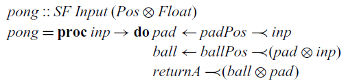
To put our bare-bones FRP library to use, let’s implement a simple single-player variant of the classic game Pong: the player has to move a paddle at the bottom of the screen to bounce a ball and prevent it from falling. Footnote 2 The core behaviour is described by the following stream function:
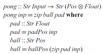
It receives a stream of inputs (button presses and how much time has passed since the last input) and produces a stream of pairs consisting of the 2D position of the ball and the x coordinate of the paddle. Its implementation uses two helper functions to compute these two components. The position of the paddle only depends on the input, whereas the position of the ball also depends on the position of the paddle (since it may bounce off it):
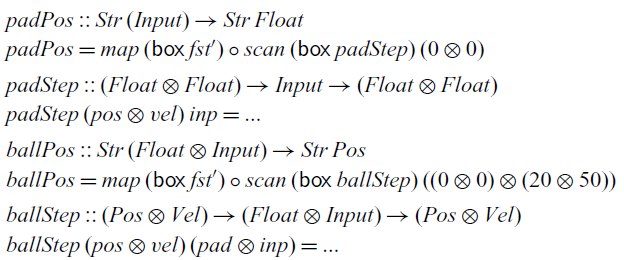
Both auxiliary functions follow the same structure. They use a $\textit{scan}$
to compute the position and the velocity of the object, while consuming the input stream. The velocity is only needed to compute the position and is therefore projected away afterward using
$\textit{scan}$
to compute the position and the velocity of the object, while consuming the input stream. The velocity is only needed to compute the position and is therefore projected away afterward using $\textit{map}$
. Here,
$\textit{map}$
. Here, ${\textit{fst}'}$
is the first projection for the strict pair type. We can see that the ball starts at the centre of the screen (at coordinates (0,0)) and moves toward the upper right corner (with velocity (20,50)).
${\textit{fst}'}$
is the first projection for the strict pair type. We can see that the ball starts at the centre of the screen (at coordinates (0,0)) and moves toward the upper right corner (with velocity (20,50)).
This simple game only requires a static dataflow network. To demonstrate the ability to express dynamically changing dataflow networks in $\mathsf{Rattus}$
, we briefly discuss three refinements of the pong game, each of which introduces different kinds of dynamic behaviours. In each case, we reuse the existing stream functions that describe the basic behaviour of the ball and the paddle, but we combine them using different combinators. Thus, these examples also demonstrate the modularity that
$\mathsf{Rattus}$
, we briefly discuss three refinements of the pong game, each of which introduces different kinds of dynamic behaviours. In each case, we reuse the existing stream functions that describe the basic behaviour of the ball and the paddle, but we combine them using different combinators. Thus, these examples also demonstrate the modularity that $\mathsf{Rattus}$
affords.
$\mathsf{Rattus}$
affords.
First refinement.
We change the implementation of $\textit{pong}$
so that it allows the player to reset the game, for example, after the ball has fallen off the screen:
$\textit{pong}$
so that it allows the player to reset the game, for example, after the ball has fallen off the screen:
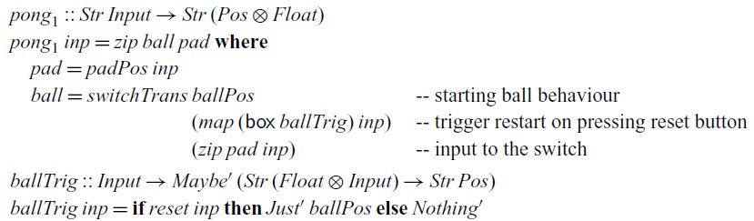
To achieve this behaviour, we use the ${\textit{switchTrans}}$
combinator, which we initialise with the original behaviour of the ball. The event that will trigger the switch is constructed by mapping
${\textit{switchTrans}}$
combinator, which we initialise with the original behaviour of the ball. The event that will trigger the switch is constructed by mapping ${\textit{ballTrig}}$
over the input stream, which will create an event of type
${\textit{ballTrig}}$
over the input stream, which will create an event of type
 ${\textit{Event}\;(\textit{Str}\;(\textit{Float}\otimes\textit{Input})\to
\textit{Str}\;\textit{Pos})}$
, which will be triggered every time the player hits the reset button.
${\textit{Event}\;(\textit{Str}\;(\textit{Float}\otimes\textit{Input})\to
\textit{Str}\;\textit{Pos})}$
, which will be triggered every time the player hits the reset button.
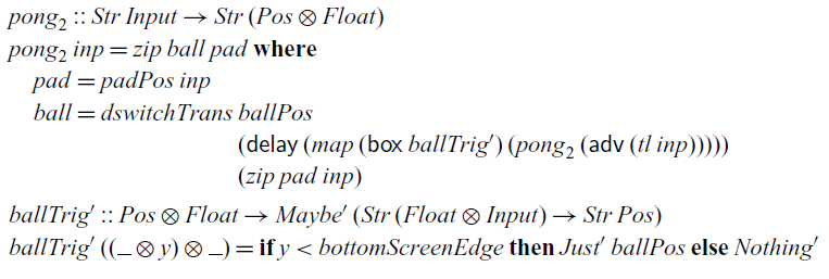
Second refinement.
Footnote 3
We can further refine this behaviour of the game so that it automatically resets once the ball has fallen off the screen. This requires a feedback loop since the behaviour of the ball depends on the current position of the ball. Such a feedback loop can be constructed using a variant of the ${\textit{switchTrans}}$
combinator that takes a delayed event as argument:
${\textit{switchTrans}}$
combinator that takes a delayed event as argument:
 \begin{equation*}
\textit{dswitchTrans}::(\textit{Str}\;a\to \textit{Str}\;b)\to \bigcirc (\textit{Event}\;(\textit{Str}\;a\to \textit{Str}\;b))\to (\textit{Str}\;a\to \textit{Str}\;b)
\end{equation*}
\begin{equation*}
\textit{dswitchTrans}::(\textit{Str}\;a\to \textit{Str}\;b)\to \bigcirc (\textit{Event}\;(\textit{Str}\;a\to \textit{Str}\;b))\to (\textit{Str}\;a\to \textit{Str}\;b)
\end{equation*}
Thus, the event we pass on to ${\textit{dswitchTrans}}$
can be constructed from the output of
${\textit{dswitchTrans}}$
can be constructed from the output of ${\textit{dswitchTrans}}$
by using guarded recursion, which closes the feedback loop:
${\textit{dswitchTrans}}$
by using guarded recursion, which closes the feedback loop:
Final refinement.
Footnote 4
Finally, we change the game a bit so as to allow the player to spawn new balls at any time and remove balls that are currently in play. To this end, we introduce a type ${\textit{ObjAction}\;a\;b}$
that represents events that may remove or add objects defined by a stream function of type
${\textit{ObjAction}\;a\;b}$
that represents events that may remove or add objects defined by a stream function of type ${\textit{Str}\;a\to \textit{Str}\;b}$
:
${\textit{Str}\;a\to \textit{Str}\;b}$
:
 \begin{equation*}
\mathbf{data}\;\textit{ObjAction}\;a\;b=\textit{Remove}\mid \textit{Add}!\!(\textit{Str}\;a\to \textit{Str}\;b)
\end{equation*}
\begin{equation*}
\mathbf{data}\;\textit{ObjAction}\;a\;b=\textit{Remove}\mid \textit{Add}!\!(\textit{Str}\;a\to \textit{Str}\;b)
\end{equation*}
To keep it simple, we only have two operations: we may add an object by giving its stream function, or we may remove the oldest object. Given the strict list type
 \begin{equation*}
\mathbf{data}\;\textit{List}\;a=\textit{Nil}\mid \textit{Cons}!\!a!\!(\textit{List}\;a)
\end{equation*}
\begin{equation*}
\mathbf{data}\;\textit{List}\;a=\textit{Nil}\mid \textit{Cons}!\!a!\!(\textit{List}\;a)
\end{equation*}
we can implement a combinator that can react to such events:
 \begin{equation*}
\textit{objTrans}::\textit{Event}\;(\textit{ObjAction}\;a\;b)\to \textit{List}\;(\textit{Str}\;b)\to \textit{Str}\;a\to \textit{Str}\;(\textit{List}\;b)
\end{equation*}
\begin{equation*}
\textit{objTrans}::\textit{Event}\;(\textit{ObjAction}\;a\;b)\to \textit{List}\;(\textit{Str}\;b)\to \textit{Str}\;a\to \textit{Str}\;(\textit{List}\;b)
\end{equation*}
This combinator takes three arguments: an event that may trigger operations to manipulate the list of active objects, the initial list of active objects, and the input stream. The result is a stream that at each step contains a list with the current value of each active object.
To use this combinator, we revise the ${\textit{ballTrig}}$
function so that it produces events to add or remove balls in response to input by the player, and we initialise the list of objects as the empty list:
${\textit{ballTrig}}$
function so that it produces events to add or remove balls in response to input by the player, and we initialise the list of objects as the empty list:
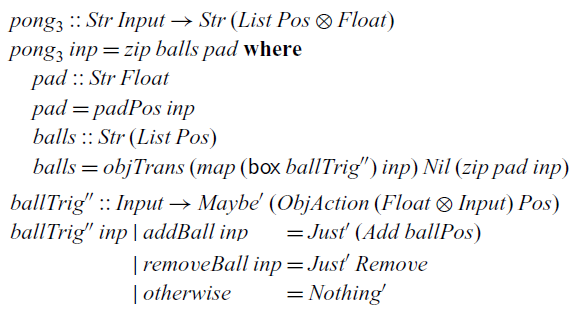
Instead of a stream of type ${\textit{Str}\;\textit{Pos}}$
to describe a single ball, we now have a stream of type
${\textit{Str}\;\textit{Pos}}$
to describe a single ball, we now have a stream of type ${\textit{Str}\;(\textit{List}\;\textit{Pos})}$
to describe multiple balls.
${\textit{Str}\;(\textit{List}\;\textit{Pos})}$
to describe multiple balls.
The ${\textit{objTrans}}$
combinator demonstrates that
${\textit{objTrans}}$
combinator demonstrates that $\mathsf{Rattus}$
can accommodate dataflow networks that dynamically grow and shrink. But more realistic variants of this combinator can be implemented as well. For example, by replacing
$\mathsf{Rattus}$
can accommodate dataflow networks that dynamically grow and shrink. But more realistic variants of this combinator can be implemented as well. For example, by replacing ${\textit{List}}$
with a
${\textit{List}}$
with a ${\textit{Map}}$
data structure, objects may have identifiers and can be removed or manipulated based on that identifier. Orthogonal to that, we may also allow objects to destroy themselves and spawn new objects. This can be achieved by describing objects using trees instead of streams:
${\textit{Map}}$
data structure, objects may have identifiers and can be removed or manipulated based on that identifier. Orthogonal to that, we may also allow objects to destroy themselves and spawn new objects. This can be achieved by describing objects using trees instead of streams:
 \begin{equation*}
\mathbf{data}\;\textit{Tree}\;a=\textit{End}\mid \textit{Next}!\!a!\!(\bigcirc (\textit{Tree}\;a))\mid \textit{Branch}!\!a!\!(\bigcirc (\textit{Tree}\;a))!\!(\bigcirc (\textit{Tree}\;a))
\end{equation*}
\begin{equation*}
\mathbf{data}\;\textit{Tree}\;a=\textit{End}\mid \textit{Next}!\!a!\!(\bigcirc (\textit{Tree}\;a))\mid \textit{Branch}!\!a!\!(\bigcirc (\textit{Tree}\;a))!\!(\bigcirc (\textit{Tree}\;a))
\end{equation*}
A variant of ${\textit{objTrans}}$
can then be implemented where the type
${\textit{objTrans}}$
can then be implemented where the type ${\textit{Str}\;b}$
in
${\textit{Str}\;b}$
in ${\textit{objTrans}}$
and
${\textit{objTrans}}$
and ${\textit{ObjAction}\;a\;b}$
is replaced by
${\textit{ObjAction}\;a\;b}$
is replaced by ${\textit{Tree}\;b}$
. For example, this can be used in the pong game to make balls destroy themselves once they disappear from screen or make a ball split into two balls when it hits a certain surface.
${\textit{Tree}\;b}$
. For example, this can be used in the pong game to make balls destroy themselves once they disappear from screen or make a ball split into two balls when it hits a certain surface.
3.3 Arrowised FRP
The benefit of a modal FRP language is that we can directly interact with signals and events in a way that guarantees causality. A popular alternative to ensure causality is arrowised FRP (Nilsson et al., Reference Nilsson, Courtney and Peterson2002), which takes signal functions as primitive and uses Haskell’s arrow notation (Paterson, Reference Paterson2001) to construct them. By implementing an arrowised FRP library in $\mathsf{Rattus}$
instead of plain Haskell, we can not only guarantee causality but also productivity and the absence of implicit space leaks. As we will see, this forces us to slightly restrict the API of arrowised FRP compared to Yampa. Furthermore, this exercise demonstrates that
$\mathsf{Rattus}$
instead of plain Haskell, we can not only guarantee causality but also productivity and the absence of implicit space leaks. As we will see, this forces us to slightly restrict the API of arrowised FRP compared to Yampa. Furthermore, this exercise demonstrates that $\mathsf{Rattus}$
can also be used to implement a continuous-time FRP library, in contrast to the discrete-time FRP library from Section 3.1.
$\mathsf{Rattus}$
can also be used to implement a continuous-time FRP library, in contrast to the discrete-time FRP library from Section 3.1.
At the centre of arrowised FRP is the ${\textit{Arrow}}$
type class shown in Figure 2. If we can implement a signal function type
${\textit{Arrow}}$
type class shown in Figure 2. If we can implement a signal function type ${\textit{SF}\;a\;b}$
that implements the
${\textit{SF}\;a\;b}$
that implements the ${\textit{Arrow}}$
class, we can benefit from the convenient notation Haskell provides for it. For example, assuming we have signal functions
${\textit{Arrow}}$
class, we can benefit from the convenient notation Haskell provides for it. For example, assuming we have signal functions ${\textit{ballPos}::\textit{SF}\;(\textit{Float}\otimes\textit{Input})\;\textit{Pos}}$
and padPos::SF Input Float describing the positions of the ball and the paddle from our game in Section 3.2, we can combine these as follows:
${\textit{ballPos}::\textit{SF}\;(\textit{Float}\otimes\textit{Input})\;\textit{Pos}}$
and padPos::SF Input Float describing the positions of the ball and the paddle from our game in Section 3.2, we can combine these as follows:
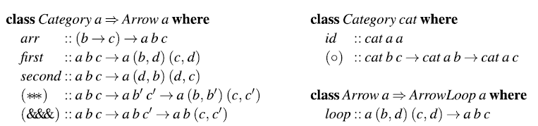
Fig. 2. Arrow type class.
The $\mathsf{Rattus}$
definition of
$\mathsf{Rattus}$
definition of ${\textit{SF}}$
is almost identical to the original Haskell definition from Nilsson et al. (Reference Nilsson, Courtney and Peterson2002). The only difference is the use of strict types and the insertion of the
${\textit{SF}}$
is almost identical to the original Haskell definition from Nilsson et al. (Reference Nilsson, Courtney and Peterson2002). The only difference is the use of strict types and the insertion of the $\bigcirc$
modality to make it a guarded recursive type:
$\bigcirc$
modality to make it a guarded recursive type:
 \begin{equation*}
\mathbf{data}\;\textit{SF}\;a\;b=\textit{SF}!(\textit{Float}\to a\to
(\bigcirc (\textit{SF}\;a\;b)\otimes b))
\end{equation*}
\begin{equation*}
\mathbf{data}\;\textit{SF}\;a\;b=\textit{SF}!(\textit{Float}\to a\to
(\bigcirc (\textit{SF}\;a\;b)\otimes b))
\end{equation*}
This implements a continuous-time signal function using sampling, where the additional argument of type ${\textit{Float}}$
indicates the time passed since the previous sample.
${\textit{Float}}$
indicates the time passed since the previous sample.
Implementing the methods of the ${\textit{Arrow}}$
type class is straightforward with the exception of the
${\textit{Arrow}}$
type class is straightforward with the exception of the ${\textit{arr}}$
method. In fact, we cannot implement
${\textit{arr}}$
method. In fact, we cannot implement ${\textit{arr}}$
in
${\textit{arr}}$
in $\mathsf{Rattus}$
at all. Because the first argument is not stable, it falls out of scope in the recursive call:
$\mathsf{Rattus}$
at all. Because the first argument is not stable, it falls out of scope in the recursive call:

The situation is similar to the $\textit{map}$
function, and we must box the function argument so that it remains available at all times in the future:
$\textit{map}$
function, and we must box the function argument so that it remains available at all times in the future:
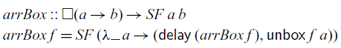
That is, the ${\textit{arr}}$
method could be a potential source for space leaks. However, in practice,
${\textit{arr}}$
method could be a potential source for space leaks. However, in practice, ${\textit{arr}}$
does not seem to cause space leaks and thus its use in conventional arrowised FRP libraries should be safe. Nonetheless, in
${\textit{arr}}$
does not seem to cause space leaks and thus its use in conventional arrowised FRP libraries should be safe. Nonetheless, in $\mathsf{Rattus}$
, we have to replace
$\mathsf{Rattus}$
, we have to replace ${\textit{arr}}$
with the more restrictive variant
${\textit{arr}}$
with the more restrictive variant ${\textit{arrBox}}$
. But fortunately, this does not prevent us from using the arrow notation:
${\textit{arrBox}}$
. But fortunately, this does not prevent us from using the arrow notation: $\mathsf{Rattus}$
treats
$\mathsf{Rattus}$
treats ${\textit{arr}\;f}$
as a short hand for
${\textit{arr}\;f}$
as a short hand for ${\textit{arrBox}\;(\mathsf{box}\;f)}$
, which allows us to use the arrow notation while making sure that
${\textit{arrBox}\;(\mathsf{box}\;f)}$
, which allows us to use the arrow notation while making sure that ${\mathsf{box}\;f}$
is well-typed, that is, f only refers to variables of stable type.
${\mathsf{box}\;f}$
is well-typed, that is, f only refers to variables of stable type.
The ${\textit{Arrow}}$
type class only provides a basic interface for constructing static signal functions. To permit dynamic behaviour, we need to provide additional combinators, for example, for switching signals and for recursive definitions. The
${\textit{Arrow}}$
type class only provides a basic interface for constructing static signal functions. To permit dynamic behaviour, we need to provide additional combinators, for example, for switching signals and for recursive definitions. The ${\textit{rSwitch}}$
combinator corresponds to the
${\textit{rSwitch}}$
combinator corresponds to the ${\textit{switchTrans}}$
combinator from Figure 1:
${\textit{switchTrans}}$
combinator from Figure 1:
 \begin{equation*}
\textit{rSwitch}::\textit{SF}\;a\;b\to \textit{SF}\;(a\otimes\textit{Maybe'}\;(\textit{SF}\;a\;b))\;b
\end{equation*}
\begin{equation*}
\textit{rSwitch}::\textit{SF}\;a\;b\to \textit{SF}\;(a\otimes\textit{Maybe'}\;(\textit{SF}\;a\;b))\;b
\end{equation*}
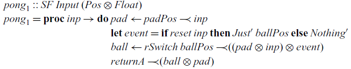
This combinator allows us to implement our game so that it resets to its start position if we hit the reset button: Footnote 5
Arrows can be endowed with a very general recursion principle by instantiating the $\textit{loop}$
method in the
$\textit{loop}$
method in the ${\textit{ArrowLoop}}$
type class shown in Figure 2. However,
${\textit{ArrowLoop}}$
type class shown in Figure 2. However, $\textit{loop}$
cannot be implemented in
$\textit{loop}$
cannot be implemented in $\mathsf{Rattus}$
as it would break the productivity property. Moreover,
$\mathsf{Rattus}$
as it would break the productivity property. Moreover, $\textit{loop}$
depends crucially on lazy evaluation and is thus a source for space leaks.
$\textit{loop}$
depends crucially on lazy evaluation and is thus a source for space leaks.
Instead of $\textit{loop}$
, we implement a different recursion principle that corresponds to guarded recursion:
$\textit{loop}$
, we implement a different recursion principle that corresponds to guarded recursion:
 \begin{equation*}
\textit{loopPre}::\textit{d}\to \textit{SF}\;(b\otimes\textit{d})\;(\textit{c}\otimes\bigcirc \textit{d})\to \textit{SF}\;b\;\textit{c}
\end{equation*}
\begin{equation*}
\textit{loopPre}::\textit{d}\to \textit{SF}\;(b\otimes\textit{d})\;(\textit{c}\otimes\bigcirc \textit{d})\to \textit{SF}\;b\;\textit{c}
\end{equation*}
Intuitively speaking, this combinator constructs a signal function from b to c with the help of an internal state of type d. The first argument initialises the state, and the second argument is a signal function that turns input of type b into output of type c while also updating the internal state. Apart from the addition of the $\bigcirc$
modality and strict pair types, this definition has the same type as Yampa’s
$\bigcirc$
modality and strict pair types, this definition has the same type as Yampa’s ${\textit{loopPre}}$
. Alternatively, we could drop the
${\textit{loopPre}}$
. Alternatively, we could drop the $\bigcirc$
modality and constrain d to be stable. The use of
$\bigcirc$
modality and constrain d to be stable. The use of ${\textit{loopPre}}$
instead of
${\textit{loopPre}}$
instead of $\textit{loop}$
introduce a delay by one sampling step (as indicated by the
$\textit{loop}$
introduce a delay by one sampling step (as indicated by the $\bigcirc$
modality) and thus ensures productivity. However, in practice, such a delay can be avoided by refactoring the underlying signal function.
$\bigcirc$
modality) and thus ensures productivity. However, in practice, such a delay can be avoided by refactoring the underlying signal function.
Using the ${\textit{loopPre}}$
combinator, we can implement the signal function of the ball:
${\textit{loopPre}}$
combinator, we can implement the signal function of the ball:
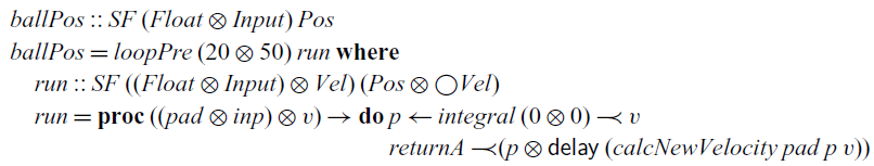
Here, we also use the ${\textit{integral}}$
combinator that computes the integral of a signal using a simple approximation that sums up rectangles under the curve:
${\textit{integral}}$
combinator that computes the integral of a signal using a simple approximation that sums up rectangles under the curve:
 \begin{equation*}
\textit{integral}::(\textit{Stable}\;a,\textit{VectorSpace}\;a\;\textit{s})\Rightarrow a\to \textit{SF}\;a\;a
\end{equation*}
\begin{equation*}
\textit{integral}::(\textit{Stable}\;a,\textit{VectorSpace}\;a\;\textit{s})\Rightarrow a\to \textit{SF}\;a\;a
\end{equation*}
The signal function for the paddle can be implemented in a similar fashion. The complete code of the case studies presented in this section can be found in the supplementary material.
4 Core calculus
In this section, we present the core calculus of $\mathsf{Rattus}$
, which we call
$\mathsf{Rattus}$
, which we call $\lambda_{\checkmark\!\!\checkmark}$
. The purpose of
$\lambda_{\checkmark\!\!\checkmark}$
. The purpose of $\lambda_{\checkmark\!\!\checkmark}$
is to formally present the language’s Fitch-style typing rules, its operational semantics, and to formally prove the central operational properties, that is, productivity, causality, and absence of implicit space leaks. To this end, the calculus is stripped down to its essence: a simply typed lambda calculus extended with guarded recursive types
$\lambda_{\checkmark\!\!\checkmark}$
is to formally present the language’s Fitch-style typing rules, its operational semantics, and to formally prove the central operational properties, that is, productivity, causality, and absence of implicit space leaks. To this end, the calculus is stripped down to its essence: a simply typed lambda calculus extended with guarded recursive types $\mathsf{Fix}\,\alpha. A$
, a guarded fixed point combinator, and the two type modalities
$\mathsf{Fix}\,\alpha. A$
, a guarded fixed point combinator, and the two type modalities $\square$
and
$\square$
and $\bigcirc $
. Since general inductive types and polymorphic types are orthogonal to the issue of operational properties in reactive programming, we have omitted these for the sake of clarity.
$\bigcirc $
. Since general inductive types and polymorphic types are orthogonal to the issue of operational properties in reactive programming, we have omitted these for the sake of clarity.
4.1 Type system
Figure 3 defines the syntax of $\lambda_{\checkmark\!\!\checkmark}$
. Besides guarded recursive types, guarded fixed points, and the two type modalities, we include standard sum and product types along with unit and integer types. The type
$\lambda_{\checkmark\!\!\checkmark}$
. Besides guarded recursive types, guarded fixed points, and the two type modalities, we include standard sum and product types along with unit and integer types. The type ${\textit{Str}\;\textit{A}}$
of streams of type A is represented as the guarded recursive type
${\textit{Str}\;\textit{A}}$
of streams of type A is represented as the guarded recursive type $\mathsf{Fix}\,\alpha. A \times \alpha$
. Note the absence of
$\mathsf{Fix}\,\alpha. A \times \alpha$
. Note the absence of $\bigcirc $
in this type. When unfolding guarded recursive types such as
$\bigcirc $
in this type. When unfolding guarded recursive types such as $\mathsf{Fix}\,\alpha. A \times \alpha$
, the
$\mathsf{Fix}\,\alpha. A \times \alpha$
, the $\bigcirc$
modality is inserted implicitly:
$\bigcirc$
modality is inserted implicitly:
 $\mathsf{Fix}\,\alpha . A \times \alpha \cong A \times \bigcirc (\mathsf{Fix}\,\alpha. A
\times \alpha)$
. This ensures that guarded recursive types are by construction always guarded by the
$\mathsf{Fix}\,\alpha . A \times \alpha \cong A \times \bigcirc (\mathsf{Fix}\,\alpha. A
\times \alpha)$
. This ensures that guarded recursive types are by construction always guarded by the $\bigcirc$
modality.
$\bigcirc$
modality.
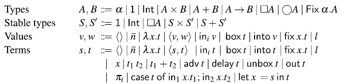
Fig. 3. Syntax of (stable) types, terms, and values. In typing rules, only closed types are considered (i.e., each occurrence of a type variable $\alpha$
is in the scope of a
$\alpha$
is in the scope of a $\mathsf{Fix}\,\alpha$
).
$\mathsf{Fix}\,\alpha$
).
For the sake of the operational semantics, the syntax also includes heap locations 1. However, as we shall see, heap locations cannot be used by the programmer directly, because there is no typing rule for them. Instead, heap locations are allocated and returned by $\mathsf{delay}$
in the operational semantics. This is a standard approach for languages with references (see e.g., Abramsky et al. (Reference Abramsky, Honda and McCusker1998); Krishnaswami (Reference Krishnaswami2013)).
$\mathsf{delay}$
in the operational semantics. This is a standard approach for languages with references (see e.g., Abramsky et al. (Reference Abramsky, Honda and McCusker1998); Krishnaswami (Reference Krishnaswami2013)).
Typing contexts, defined in Figure 4, consist of variable typings $x:A$
and
$x:A$
and $\checkmark$
tokens. If a typing context contains no
$\checkmark$
tokens. If a typing context contains no $\checkmark$
, we call it tick-free. The complete set of typing rules for
$\checkmark$
, we call it tick-free. The complete set of typing rules for $\lambda_{\checkmark\!\!\checkmark}$
is given in Figure 5. The typing rules for
$\lambda_{\checkmark\!\!\checkmark}$
is given in Figure 5. The typing rules for $\mathsf{Rattus}$
presented in Section 2 appear in the same form also here, except for replacing Haskell’s :: operator with the more standard notation. The remaining typing rules are entirely standard, except for the typing rule for the guarded fixed point combinator
$\mathsf{Rattus}$
presented in Section 2 appear in the same form also here, except for replacing Haskell’s :: operator with the more standard notation. The remaining typing rules are entirely standard, except for the typing rule for the guarded fixed point combinator $\mathsf{fix}$
.
$\mathsf{fix}$
.
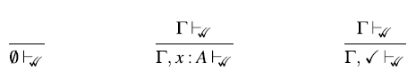
Fig. 4. Well-formed contexts.
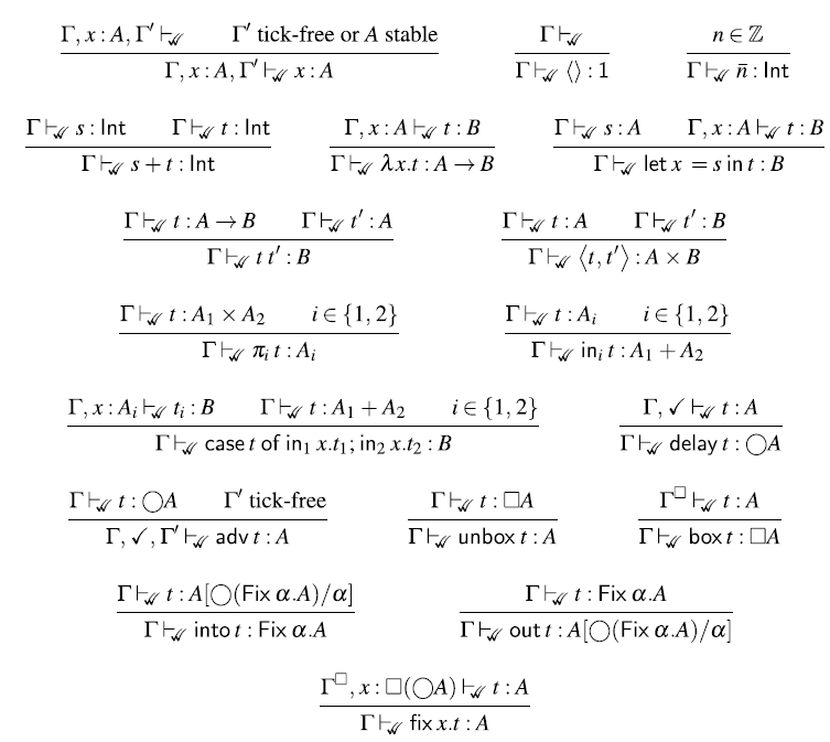
Fig. 5. Typing rules.
The typing rule for $\mathsf{fix}$
follows Nakano’s fixed point combinator and ensures that the calculus is productive. In addition, following Krishnaswami (Reference Krishnaswami2013), the rule enforces the body t of the fixed point to be stable by strengthening the typing context to
$\mathsf{fix}$
follows Nakano’s fixed point combinator and ensures that the calculus is productive. In addition, following Krishnaswami (Reference Krishnaswami2013), the rule enforces the body t of the fixed point to be stable by strengthening the typing context to $\Gamma^{\square}$
. Moreover, we follow Bahr et al. (Reference Bahr, Graulund and Møgelberg2021) and assume x to be of type
$\Gamma^{\square}$
. Moreover, we follow Bahr et al. (Reference Bahr, Graulund and Møgelberg2021) and assume x to be of type ${\square(\bigcirc \textit{A})}$
instead of
${\square(\bigcirc \textit{A})}$
instead of ${\bigcirc \textit{A}}$
. As a consequence, recursive calls may occur at any time in the future, that is, not necessarily in the very next time step. In conjunction with the more general typing rule for
${\bigcirc \textit{A}}$
. As a consequence, recursive calls may occur at any time in the future, that is, not necessarily in the very next time step. In conjunction with the more general typing rule for $\mathsf{delay}$
, this allows us to write recursive function definitions that, like
$\mathsf{delay}$
, this allows us to write recursive function definitions that, like $\textit{stutter}$
in Section 2.2, look several steps into the future.
$\textit{stutter}$
in Section 2.2, look several steps into the future.
To see how the recursion syntax of $\mathsf{Rattus}$
translates into the fixed point combinator of
$\mathsf{Rattus}$
translates into the fixed point combinator of $\lambda_{\checkmark\!\!\checkmark}$
, let us reconsider the
$\lambda_{\checkmark\!\!\checkmark}$
, let us reconsider the $\textit{constInt}$
function:
$\textit{constInt}$
function:
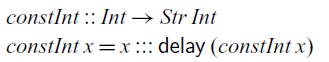
For readability of the corresponding $\lambda_{\checkmark\!\!\checkmark}$
term, we use the shorthand
$\lambda_{\checkmark\!\!\checkmark}$
term, we use the shorthand $s ::: t$
for the
$s ::: t$
for the $\lambda_{\checkmark\!\!\checkmark}$
term
$\lambda_{\checkmark\!\!\checkmark}$
term
 $\mathsf{into}
\langle{s}{t}\rangle$
. Recall that
$\mathsf{into}
\langle{s}{t}\rangle$
. Recall that ${\textit{Str}\;\textit{A}}$
is represented as
${\textit{Str}\;\textit{A}}$
is represented as $\mathsf{Fix}\,\alpha. A \times \alpha$
in
$\mathsf{Fix}\,\alpha. A \times \alpha$
in $\lambda_{\checkmark\!\!\checkmark}$
. That is, given
$\lambda_{\checkmark\!\!\checkmark}$
. That is, given $s : A$
and
$s : A$
and $t : \bigcirc ({\textit{Str}\;\textit{A}})$
, we have that
$t : \bigcirc ({\textit{Str}\;\textit{A}})$
, we have that $s ::: t$
is of type
$s ::: t$
is of type ${\textit{Str}\;\textit{A}}$
. Using this notation, the above definition translates into the following
${\textit{Str}\;\textit{A}}$
. Using this notation, the above definition translates into the following $\lambda_{\checkmark\!\!\checkmark}$
term:
$\lambda_{\checkmark\!\!\checkmark}$
term:
 \begin{equation*}
\mathit{constInt} = \mathsf{fix}\, r. \lambda x . x ::: \mathsf{delay} (\mathsf{adv}\, (\mathsf{unbox}\, r)\,x)
\end{equation*}
\begin{equation*}
\mathit{constInt} = \mathsf{fix}\, r. \lambda x . x ::: \mathsf{delay} (\mathsf{adv}\, (\mathsf{unbox}\, r)\,x)
\end{equation*}
The recursive notation is simply translated into a fixed point $\mathsf{Fix}\,r. t$
where the recursive occurrence of
$\mathsf{Fix}\,r. t$
where the recursive occurrence of $\textit{constInt}$
is replaced by
$\textit{constInt}$
is replaced by ${\mathsf{adv}\;(\mathsf{unbox}\;\textit{r})}$
. The variable r is of type
${\mathsf{adv}\;(\mathsf{unbox}\;\textit{r})}$
. The variable r is of type ${\square(\bigcirc (\textit{Int}\to \textit{Str}\;\textit{Int}))}$
and applying
${\square(\bigcirc (\textit{Int}\to \textit{Str}\;\textit{Int}))}$
and applying $\mathsf{unbox}$
followed by
$\mathsf{unbox}$
followed by $\mathsf{adv}$
turns it into type
$\mathsf{adv}$
turns it into type ${\textit{Int}\to \textit{Str}\;\textit{Int}}$
. Moreover, the restriction that recursive calls must occur in a context with
${\textit{Int}\to \textit{Str}\;\textit{Int}}$
. Moreover, the restriction that recursive calls must occur in a context with $\checkmark$
makes sure that this transformation from recursion notation to fixed point combinator results in a well-typed
$\checkmark$
makes sure that this transformation from recursion notation to fixed point combinator results in a well-typed $\lambda_{\checkmark\!\!\checkmark}$
term.
$\lambda_{\checkmark\!\!\checkmark}$
term.
The typing rule for $\mathsf{fix}\,x. t$
also explains the treatment of recursive definitions that are nested inside a top-level definition. The typing context
$\mathsf{fix}\,x. t$
also explains the treatment of recursive definitions that are nested inside a top-level definition. The typing context $\Gamma$
is turned into
$\Gamma$
is turned into $\Gamma^{\square}$
when type-checking the body t of the fixed point.
$\Gamma^{\square}$
when type-checking the body t of the fixed point.
For example, reconsider the following ill-typed definition of ${\textit{leakyMap}}:$
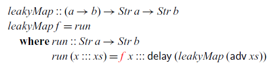
Translated into $\lambda_{\checkmark\!\!\checkmark}$
, the definition looks like this:
$\lambda_{\checkmark\!\!\checkmark}$
, the definition looks like this:
 \begin{align*}
\mathit{leakyMap} = \lambda f. \mathsf{fix}\, r. \lambda s. &\mathsf{let}\, x =
\mathsf{head}\,s\;\mathsf{in}\,\mathsf{let}\,xs = \mathsf{tail}\,
s\\
&\mathsf{in}\;{\color{red}f}\, x ::: \mathsf{delay} ((\mathsf{adv}\, (\mathsf{unbox}\,r))\,(\mathsf{adv}\,xs))
\end{align*}
\begin{align*}
\mathit{leakyMap} = \lambda f. \mathsf{fix}\, r. \lambda s. &\mathsf{let}\, x =
\mathsf{head}\,s\;\mathsf{in}\,\mathsf{let}\,xs = \mathsf{tail}\,
s\\
&\mathsf{in}\;{\color{red}f}\, x ::: \mathsf{delay} ((\mathsf{adv}\, (\mathsf{unbox}\,r))\,(\mathsf{adv}\,xs))
\end{align*}
The pattern matching syntax is translated into projection functions $\mathsf{head}$
and
$\mathsf{head}$
and $\mathsf{tail}$
that decompose a stream into its head and tail, respectively, that is,
$\mathsf{tail}$
that decompose a stream into its head and tail, respectively, that is,
 \begin{equation*}
\mathsf{head} = \lambda x . \pi_1\,(\mathsf{out}\,x) \qquad \mathsf{tail}
= \lambda x . \pi_2\,(\mathsf{out}\,x)
\end{equation*}
\begin{equation*}
\mathsf{head} = \lambda x . \pi_1\,(\mathsf{out}\,x) \qquad \mathsf{tail}
= \lambda x . \pi_2\,(\mathsf{out}\,x)
\end{equation*}
More importantly, the variable f bound by the outer lambda abstraction is of a function type and thus not stable. Therefore, it is not in scope in the body of the fixed point.
4.2 Operational semantics
The operational semantics is given in two steps: to execute a $\lambda_{\checkmark\!\!\checkmark}$
program, it is first translated into a more restrictive variant of
$\lambda_{\checkmark\!\!\checkmark}$
program, it is first translated into a more restrictive variant of $\lambda_{\checkmark\!\!\checkmark}$
, which we call
$\lambda_{\checkmark\!\!\checkmark}$
, which we call $\lambda_{\checkmark}$
. The resulting
$\lambda_{\checkmark}$
. The resulting $\lambda_{\checkmark}$
program is then executed using an abstract machine that ensures the absence of implicit space leaks by construction. By presenting the operational semantics in two stages, we avoid the more complicated set-up of an abstract machine that is capable of directly executing
$\lambda_{\checkmark}$
program is then executed using an abstract machine that ensures the absence of implicit space leaks by construction. By presenting the operational semantics in two stages, we avoid the more complicated set-up of an abstract machine that is capable of directly executing $\lambda_{\checkmark\!\!\checkmark}$
programs. As we show in the example in Section 4.3.3, such a machine would need to perform some restricted form of partial evaluation under
$\lambda_{\checkmark\!\!\checkmark}$
programs. As we show in the example in Section 4.3.3, such a machine would need to perform some restricted form of partial evaluation under $\mathsf{delay}$
and under lambda abstractions.
$\mathsf{delay}$
and under lambda abstractions.
4.2.1 Translation to $\lambda_{\checkmark}$

The $\lambda_{\checkmark}$
calculus has the same syntax as
$\lambda_{\checkmark}$
calculus has the same syntax as $\lambda_{\checkmark\!\!\checkmark}$
, but the former has a more restrictive type system. It restricts typing contexts to contain at most one
$\lambda_{\checkmark\!\!\checkmark}$
, but the former has a more restrictive type system. It restricts typing contexts to contain at most one $\checkmark$
and restricts the typing rules for lambda abstraction and
$\checkmark$
and restricts the typing rules for lambda abstraction and $\mathsf{delay}$
as follows:
$\mathsf{delay}$
as follows:
The construction $\vert{\Gamma}\vert$
turns
$\vert{\Gamma}\vert$
turns $\Gamma$
into a tick-free context, which ensures that we have at most one
$\Gamma$
into a tick-free context, which ensures that we have at most one $\checkmark$
– even for nested occurrences of
$\checkmark$
– even for nested occurrences of $\mathsf{delay}$
– and that the body of a lambda abstraction is not in the scope of a
$\mathsf{delay}$
– and that the body of a lambda abstraction is not in the scope of a $\checkmark$
. All other typing rules are the same as for
$\checkmark$
. All other typing rules are the same as for $\lambda_{\checkmark\!\!\checkmark}$
. The
$\lambda_{\checkmark\!\!\checkmark}$
. The $\lambda_{\checkmark}$
calculus is a fragment of the
$\lambda_{\checkmark}$
calculus is a fragment of the $\lambda_{\checkmark\!\!\checkmark}$
calculus in the sense that
$\lambda_{\checkmark\!\!\checkmark}$
calculus in the sense that $\Gamma\vdash_{\!\checkmark}{t}{A}$
implies
$\Gamma\vdash_{\!\checkmark}{t}{A}$
implies $\Gamma\vdash_{\!\checkmark}{t}{A}$
.
$\Gamma\vdash_{\!\checkmark}{t}{A}$
.
Any closed $\lambda_{\checkmark\!\!\checkmark}$
term can be translated into a corresponding
$\lambda_{\checkmark\!\!\checkmark}$
term can be translated into a corresponding $\lambda_{\checkmark}$
term by exhaustively applying the following rewrite rules:
$\lambda_{\checkmark}$
term by exhaustively applying the following rewrite rules:
where K is a term with a single hole that does not occur in the scope of $\mathsf{delay}$
,
$\mathsf{delay}$
, $\mathsf{adv}$
,
$\mathsf{adv}$
, $\mathsf{box}$
,
$\mathsf{box}$
, $\mathsf{fix}$
, or lambda abstraction; and K[t] is the term obtained from K by replacing its hole with the term t.
$\mathsf{fix}$
, or lambda abstraction; and K[t] is the term obtained from K by replacing its hole with the term t.
For example, consider the closed $\lambda_{\checkmark\!\!\checkmark}$
term
$\lambda_{\checkmark\!\!\checkmark}$
term $\lambda f.\mathsf{delay}(\lambda x. \mathsf{adv}\,(\mathsf{unbox}\,f)\, (x+1))$
of type
$\lambda f.\mathsf{delay}(\lambda x. \mathsf{adv}\,(\mathsf{unbox}\,f)\, (x+1))$
of type $\square\bigcirc ({\rm Int} \to {\rm Int}) \to \bigcirc ({\rm Int} \to {\rm Int})$
. Applying the second rewrite rule followed by the first rewrite rule, this term rewrites to a
$\square\bigcirc ({\rm Int} \to {\rm Int}) \to \bigcirc ({\rm Int} \to {\rm Int})$
. Applying the second rewrite rule followed by the first rewrite rule, this term rewrites to a $\lambda_{\checkmark}$
term of the same type as follows:
$\lambda_{\checkmark}$
term of the same type as follows:
 \begin{align*}
&\lambda f.\mathsf{delay}(\lambda x. \mathsf{adv} \,(\mathsf{unbox}\,f)\, (x+1))\\
\to\ & \lambda f.\mathsf{delay}({\rm let}\, y {\mathsf{adv}\, (\mathsf{unbox}\,f)} {\lambda x. y\, (x+1)})\\
\to\ & \lambda f.{\rm let}\, z {\mathsf{unbox}\,f}{\mathsf{delay}({\rm
let}\, y {\mathsf{adv}\, z} {\lambda x. y\, (x+1)})}
\end{align*}
\begin{align*}
&\lambda f.\mathsf{delay}(\lambda x. \mathsf{adv} \,(\mathsf{unbox}\,f)\, (x+1))\\
\to\ & \lambda f.\mathsf{delay}({\rm let}\, y {\mathsf{adv}\, (\mathsf{unbox}\,f)} {\lambda x. y\, (x+1)})\\
\to\ & \lambda f.{\rm let}\, z {\mathsf{unbox}\,f}{\mathsf{delay}({\rm
let}\, y {\mathsf{adv}\, z} {\lambda x. y\, (x+1)})}
\end{align*}
In a well-typed $\lambda_{\checkmark\!\!\checkmark}$
term, each subterm
$\lambda_{\checkmark\!\!\checkmark}$
term, each subterm $\mathsf{adv}\,t$
must occur in the scope of a corresponding
$\mathsf{adv}\,t$
must occur in the scope of a corresponding $\mathsf{delay}$
. The above rewrite rules make sure that the subterm t is evaluated before the
$\mathsf{delay}$
. The above rewrite rules make sure that the subterm t is evaluated before the $\mathsf{delay}$
. This corresponds to the intuition that
$\mathsf{delay}$
. This corresponds to the intuition that $\mathsf{delay}$
moves ahead in time and
$\mathsf{delay}$
moves ahead in time and $\mathsf{adv}$
moves back in time – thus the two cancel out one another.
$\mathsf{adv}$
moves back in time – thus the two cancel out one another.
One can show that the rewrite rules are strongly normalising and type-preserving (in $\lambda_{\checkmark\!\!\checkmark}$
). Moreover, any closed term in
$\lambda_{\checkmark\!\!\checkmark}$
). Moreover, any closed term in $\lambda_{\checkmark\!\!\checkmark}$
that cannot be further rewritten is also well-typed in
$\lambda_{\checkmark\!\!\checkmark}$
that cannot be further rewritten is also well-typed in $\lambda_{\checkmark}$
. As a consequence, we can exhaustively apply the rewrite rules to a closed term of
$\lambda_{\checkmark}$
. As a consequence, we can exhaustively apply the rewrite rules to a closed term of $\lambda_{\checkmark\!\!\checkmark}$
to transform it into a closed term of
$\lambda_{\checkmark\!\!\checkmark}$
to transform it into a closed term of $\lambda_{\checkmark}$
:
$\lambda_{\checkmark}$
:
Theorem 4.1 For each $\vdash_{\checkmark\!\!\checkmark}\,{t}:{A}$
, we can effectively construct a term t’ with
$\vdash_{\checkmark\!\!\checkmark}\,{t}:{A}$
, we can effectively construct a term t’ with $t \to^* t'$
and
$t \to^* t'$
and $\vdash_{\!\checkmark}{t'}:{A}$
.
$\vdash_{\!\checkmark}{t'}:{A}$
.
Below we give a brief overview of the three components of the proof of Theorem 4.1. For the full proof, we refer the reader to Appendix A.
Strong normalisation.
To show that $\to$
is strongly normalising, we define for each term t a natural number d(t) such that, whenever
$\to$
is strongly normalising, we define for each term t a natural number d(t) such that, whenever $t \to t'$
, then
$t \to t'$
, then $d(t) > d(t')$
. We define d(t) to be the sum of the depth of all redex occurrences in t (i.e., subterms that match the left-hand side of a rewrite rule). Since each rewrite step
$d(t) > d(t')$
. We define d(t) to be the sum of the depth of all redex occurrences in t (i.e., subterms that match the left-hand side of a rewrite rule). Since each rewrite step $t \to t'$
removes a redex or replaces a redex with a new redex at a strictly smaller depth, we have that
$t \to t'$
removes a redex or replaces a redex with a new redex at a strictly smaller depth, we have that $d(t) > d(t')$
.
$d(t) > d(t')$
.
Subject reduction.
We want to prove that $\Gamma\vdash_{\!\!\checkmark\!\!\checkmark}\,s:A$
and
$\Gamma\vdash_{\!\!\checkmark\!\!\checkmark}\,s:A$
and $s \to t$
implies
$s \to t$
implies $\Gamma\vdash_{\!\!\checkmark\!\!\checkmark}\,t:A$
. To this end, we proceed by induction on
$\Gamma\vdash_{\!\!\checkmark\!\!\checkmark}\,t:A$
. To this end, we proceed by induction on $s \to t$
. In case the reduction
$s \to t$
. In case the reduction $s \longrightarrow t$
is due to congruence closure,
$s \longrightarrow t$
is due to congruence closure, $\Gamma\vdash_{\!\!\checkmark\!\!\checkmark}\,t:A$
follows immediately by the induction hypothesis. Otherwise, s matches the left-hand side of one of the rewrite rules. Each of these two cases follows from the induction hypothesis and one of the following two properties:
$\Gamma\vdash_{\!\!\checkmark\!\!\checkmark}\,t:A$
follows immediately by the induction hypothesis. Otherwise, s matches the left-hand side of one of the rewrite rules. Each of these two cases follows from the induction hypothesis and one of the following two properties:
-
(1) If
$\Gamma,\checkmark,\Gamma'\vdash_{\!\!\checkmark\!\!\checkmark}{K[\mathsf{adv}\,t]}{A}$
and
$\Gamma'$
tick-free, then
$\Gamma\vdash_{\!\!\checkmark\!\!\checkmark}\,t{\bigcirc B}$
and
$\Gamma,x:\bigcirc B, \checkmark,\Gamma'\vdash_{\!\!\checkmark\!\!\checkmark}{K[\mathsf{adv}\,x]}{A}$
for some B. -
(2) If
$\Gamma,
\Gamma'\vdash_{\!\!\checkmark\!\!\checkmark}{K[\mathsf{adv}\,t]}:{A}$
and
$\Gamma'$
tick-free, then
$\Gamma\vdash_{\!\!\checkmark\!\!\checkmark}\mathsf{adv}\,t:B$
and
$\Gamma,x : B,\Gamma'\vdash_{\!\!\checkmark\!\!\checkmark}{K[x]}:{A}$
for some B.


Both properties can be proved by a straightforward induction on K. The proofs rely on the fact that due to the typing rule for $\mathsf{adv}$
, we know that if
$\mathsf{adv}$
, we know that if $\Gamma, \Gamma'\vdash_{\!\!\checkmark\!\!\checkmark}{K[\mathsf{adv}\,t]}:{A}$
for a tick-free
$\Gamma, \Gamma'\vdash_{\!\!\checkmark\!\!\checkmark}{K[\mathsf{adv}\,t]}:{A}$
for a tick-free $\Gamma'$
, then all of t’s free variables must be in
$\Gamma'$
, then all of t’s free variables must be in $\Gamma$
.
$\Gamma$
.
Exhaustiveness.
Finally, we need to show that $\vdash_{\!\!\checkmark\!\!\checkmark}t:A$
with
$\vdash_{\!\!\checkmark\!\!\checkmark}t:A$
with
![]() implies
implies $\vdash_{\!\checkmark}{t}:{A}$
, that is, if we cannot rewrite t any further it must be typable in
$\vdash_{\!\checkmark}{t}:{A}$
, that is, if we cannot rewrite t any further it must be typable in $\lambda_{\checkmark}$
as well. In order to prove this property by induction, we must generalise it to open terms: if
$\lambda_{\checkmark}$
as well. In order to prove this property by induction, we must generalise it to open terms: if $\Gamma\vdash_{\!\!\checkmark\!\!\checkmark}{t}:{A}$
for a context
$\Gamma\vdash_{\!\!\checkmark\!\!\checkmark}{t}:{A}$
for a context $\Gamma$
with at most one tick and
$\Gamma$
with at most one tick and
![]() , then
, then ${\Gamma}\vdash_{\!\checkmark}{t}:{A}$
. We prove this implication by induction on t and a case distinction on the last typing rule in the derivation of
${\Gamma}\vdash_{\!\checkmark}{t}:{A}$
. We prove this implication by induction on t and a case distinction on the last typing rule in the derivation of ${\Gamma}\vdash_{\!\checkmark}{t}:{A}$
. For almost all cases,
${\Gamma}\vdash_{\!\checkmark}{t}:{A}$
. For almost all cases, ${\Gamma}\vdash_{\!\checkmark}{t}:{A}$
follows from the induction hypothesis since we find a corresponding typing rule in
${\Gamma}\vdash_{\!\checkmark}{t}:{A}$
follows from the induction hypothesis since we find a corresponding typing rule in $\lambda_{\checkmark}$
that is either the same as in
$\lambda_{\checkmark}$
that is either the same as in $\lambda_{\checkmark\!\!\checkmark}$
or has a side condition is satisfied by our assumption that
$\lambda_{\checkmark\!\!\checkmark}$
or has a side condition is satisfied by our assumption that $\Gamma$
have at most one tick. We are thus left with two interesting cases: the typing rules for
$\Gamma$
have at most one tick. We are thus left with two interesting cases: the typing rules for $\mathsf{delay}$
and lambda abstraction, given that
$\mathsf{delay}$
and lambda abstraction, given that $\Gamma$
contains exactly one tick (the zero-tick cases are trivial). Each of these two cases follows from the induction hypothesis and one of the following two properties:
$\Gamma$
contains exactly one tick (the zero-tick cases are trivial). Each of these two cases follows from the induction hypothesis and one of the following two properties:
-
(1) If
${\Gamma_1,\checkmark,\Gamma_2}\vdash_{\checkmark\!\!\checkmark}{t}:{A}$
,
$\Gamma_2$
contains a tick, and
, then
$\Gamma_1^\square,\Gamma_2\vdash_{\checkmark\!\!\checkmark}{t}:{A}$
. -
(2) If
$\Gamma_1,\checkmark,\Gamma_2\vdash{t}:{A}$
and
, then
$\Gamma_1^\square,\Gamma_2\vdash_{\checkmark}{t}:{A}$
.


Both properties can be proved by a straightforward induction on the typing derivation. The proof of (1) uses the fact that t cannot have nested occurrences of $\mathsf{adv}$
and thus any occurrence of
$\mathsf{adv}$
and thus any occurrence of $\mathsf{adv}$
only needs the tick that is already present in
$\mathsf{adv}$
only needs the tick that is already present in $\Gamma_2$
. In turn, (2) holds due to the fact that all occurrences of
$\Gamma_2$
. In turn, (2) holds due to the fact that all occurrences of $\mathsf{adv}$
in t must be guarded by an occurrence of
$\mathsf{adv}$
in t must be guarded by an occurrence of $\mathsf{delay}$
in t itself, and thus the tick between
$\mathsf{delay}$
in t itself, and thus the tick between $\Gamma_1$
and
$\Gamma_1$
and $\Gamma_2$
is not needed. Note that (2) is about
$\Gamma_2$
is not needed. Note that (2) is about $\lambda_{\checkmark}$
as we first apply the induction hypothesis and then apply (2).
$\lambda_{\checkmark}$
as we first apply the induction hypothesis and then apply (2).
4.2.2 Abstract machine for
$\lambda_{\checkmark}$

To prove the absence of implicit space leaks, we devise an abstract machine that after each time step deletes all data from the previous time step. That means, the operational semantics is by construction free of implicit space leaks. This approach, pioneered by Krishnaswami (Reference Krishnaswami2013), allows us to reduce the proof of no implicit space leaks to a proof of type soundness.
At the centre of this approach is the idea to execute programs in a machine that has access to a store consisting of up to two separate heaps: a ‘now’ heap from which we can retrieve delayed computations, and a ‘later’ heap where we must store computations that should be performed in the next time step. Once the machine advances to the next time step, it will delete the ‘now’ heap and the ‘later’ heap will become the new ‘now’ heap.
The machine consists of two components: the evaluation semantics, presented in Figure 6, which describes the operational behaviour of $\lambda_{\checkmark}$
within a single time step; and the step semantics, presented in Figure 7, which describes the behaviour of a program over time, for example, how it consumes and constructs streams.
$\lambda_{\checkmark}$
within a single time step; and the step semantics, presented in Figure 7, which describes the behaviour of a program over time, for example, how it consumes and constructs streams.
Fig. 6. Evaluation semantics.
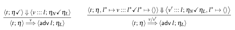
Fig. 7. Step semantics for streams.
The evaluation semantics is given as a deterministic big-step operational semantics, where we write $\left\langle t; \sigma \right\rangle \Downarrow \langle v; \sigma'\rangle$
to indicate that starting with the store
$\left\langle t; \sigma \right\rangle \Downarrow \langle v; \sigma'\rangle$
to indicate that starting with the store $\sigma$
, the term t evaluates to the value v and the new store
$\sigma$
, the term t evaluates to the value v and the new store $\sigma'$
. A store
$\sigma'$
. A store $\sigma$
can be of one of two forms: either it consists of a single heap
$\sigma$
can be of one of two forms: either it consists of a single heap $\eta_L$
, that is,
$\eta_L$
, that is, $\sigma = \eta_L$
, or it consists of two heaps
$\sigma = \eta_L$
, or it consists of two heaps $\eta_N$
and
$\eta_N$
and $\eta_L$
, written
$\eta_L$
, written $\sigma = \eta_N\checkmark\eta_L$
. The ‘later’ heap
$\sigma = \eta_N\checkmark\eta_L$
. The ‘later’ heap $\eta_L$
contains delayed computations that may be retrieved and executed in the next time step, whereas the ‘now’ heap
$\eta_L$
contains delayed computations that may be retrieved and executed in the next time step, whereas the ‘now’ heap $\eta_N$
contains delayed computations from the previous time step that can be retrieved and executed now. We can only write to
$\eta_N$
contains delayed computations from the previous time step that can be retrieved and executed now. We can only write to $\eta_L$
and only read from
$\eta_L$
and only read from $\eta_N$
. However, when one time step passes, the ‘now’ heap
$\eta_N$
. However, when one time step passes, the ‘now’ heap $\eta_N$
is deleted and the ‘later’ heap
$\eta_N$
is deleted and the ‘later’ heap $\eta_L$
becomes the new ‘now’ heap. This shifting of time is part of the step semantics in Figure 7, which we turn to shortly.
$\eta_L$
becomes the new ‘now’ heap. This shifting of time is part of the step semantics in Figure 7, which we turn to shortly.
Heaps are simply finite mappings from heap locations to terms. To allocate fresh heap locations, we assume a function $\mathsf{alloc}\cdot$
that takes a store
$\mathsf{alloc}\cdot$
that takes a store $\sigma$
of the form
$\sigma$
of the form $\eta_L$
or
$\eta_L$
or $\eta_N\checkmark\eta_L$
and returns a heap location l that is not in the domain of
$\eta_N\checkmark\eta_L$
and returns a heap location l that is not in the domain of $\eta_L$
. Given such a fresh heap location l and a term t, we write
$\eta_L$
. Given such a fresh heap location l and a term t, we write $\sigma,l\mapsto t$
to denote the store
$\sigma,l\mapsto t$
to denote the store $\eta'_L$
or
$\eta'_L$
or $\eta_N\checkmark\eta'_L$
, respectively, where
$\eta_N\checkmark\eta'_L$
, respectively, where $\eta'_L = \eta_L,l \mapsto t$
, that is,
$\eta'_L = \eta_L,l \mapsto t$
, that is, $\eta'_L$
is obtained from
$\eta'_L$
is obtained from $\eta_L$
by extending it with a new mapping
$\eta_L$
by extending it with a new mapping $l \mapsto t$
.
$l \mapsto t$
.
Applying $\mathsf{delay}$
to a term t stores t in a fresh location l on the ‘later’ heap and then returns l. Conversely, if we apply
$\mathsf{delay}$
to a term t stores t in a fresh location l on the ‘later’ heap and then returns l. Conversely, if we apply ![]() to such a delayed computation, we retrieve the term from the ‘now’ heap and evaluate it.
to such a delayed computation, we retrieve the term from the ‘now’ heap and evaluate it.
4.3 Main results
In this section, we present the main metatheoretical results. Namely, that the core calculus $\lambda_{\checkmark}$
enjoys the desired productivity, causality, and memory properties (see Theorem 4.2 and Theorem 4.3 below). The proof of these results is sketched in Section 5 and is fully mechanised in the accompanying Coq proofs. In order to formulate and prove these metatheoretical results, we devise a step semantics that describes the behaviour of reactive programs. Here, we consider two kinds of reactive programs: terms of type
$\lambda_{\checkmark}$
enjoys the desired productivity, causality, and memory properties (see Theorem 4.2 and Theorem 4.3 below). The proof of these results is sketched in Section 5 and is fully mechanised in the accompanying Coq proofs. In order to formulate and prove these metatheoretical results, we devise a step semantics that describes the behaviour of reactive programs. Here, we consider two kinds of reactive programs: terms of type ${\textit{Str}\;\textit{A}}$
and terms of type
${\textit{Str}\;\textit{A}}$
and terms of type ${\textit{Str}\;\textit{A}\to \textit{Str}\;\textit{B}}$
. The former just produce infinite streams of values of type A, whereas the latter are reactive processes that produce a value of type
${\textit{Str}\;\textit{A}\to \textit{Str}\;\textit{B}}$
. The former just produce infinite streams of values of type A, whereas the latter are reactive processes that produce a value of type ${\textit{B}}$
for each input value of type A. The purpose of the step semantics is to formulate clear metatheoretical properties and to subsequently prove them using the fundamental property of our logical relation (Theorem 5.1). In principle, we could formulate similar step semantics for the Yampa-style signal functions from Section 3.3 or other basic FRP types such as resumptions (Krishnaswami, Reference Krishnaswami2013) and then derive similar metatheoretical results.
${\textit{B}}$
for each input value of type A. The purpose of the step semantics is to formulate clear metatheoretical properties and to subsequently prove them using the fundamental property of our logical relation (Theorem 5.1). In principle, we could formulate similar step semantics for the Yampa-style signal functions from Section 3.3 or other basic FRP types such as resumptions (Krishnaswami, Reference Krishnaswami2013) and then derive similar metatheoretical results.
4.3.1 Productivity of streams
The step semantics $\overset v\Longrightarrow$
from Figure 7 describes the unfolding of streams of type
$\overset v\Longrightarrow$
from Figure 7 describes the unfolding of streams of type ${\textit{Str}\;\textit{A}}$
. Given a closed term
${\textit{Str}\;\textit{A}}$
. Given a closed term $\vdash_{\!\checkmark}{t}\textit{Str}\, A$
, it produces an infinite reduction sequence
$\vdash_{\!\checkmark}{t}\textit{Str}\, A$
, it produces an infinite reduction sequence
 \begin{equation*}
\langle{t};{\emptyset}\rangle {\overset{v_0}\Longrightarrow}
\langle{t_1};{\eta_1}{\overset{v_1}\Longrightarrow}
\langle{t_2};{\eta_2}\rangle
{\overset{v_2}\Longrightarrow} \ldots
\end{equation*}
\begin{equation*}
\langle{t};{\emptyset}\rangle {\overset{v_0}\Longrightarrow}
\langle{t_1};{\eta_1}{\overset{v_1}\Longrightarrow}
\langle{t_2};{\eta_2}\rangle
{\overset{v_2}\Longrightarrow} \ldots
\end{equation*}
where $\emptyset$
denotes the empty heap and each
$\emptyset$
denotes the empty heap and each $v_i$
has type A. In each step, we have a term
$v_i$
has type A. In each step, we have a term $t_i$
and the corresponding heap
$t_i$
and the corresponding heap $\eta_i$
of delayed computations. According to the definition of the step semantics, we evaluate
$\eta_i$
of delayed computations. According to the definition of the step semantics, we evaluate
 $\langle{t_i}{\eta_i\checkmark\rangle}\Downarrow\langle{v_i :::
l}{\eta'_i\checkmark\eta_{i+1}\rangle}$
, where
$\langle{t_i}{\eta_i\checkmark\rangle}\Downarrow\langle{v_i :::
l}{\eta'_i\checkmark\eta_{i+1}\rangle}$
, where $\eta'_i$
is
$\eta'_i$
is $\eta_i$
but possibly extended with some additional delayed computations and
$\eta_i$
but possibly extended with some additional delayed computations and $\eta_{i+1}$
is the new heap with delayed computations for the next time step. Crucially, the old heap
$\eta_{i+1}$
is the new heap with delayed computations for the next time step. Crucially, the old heap $\eta'_i$
is thrown away. That is, by construction, old data is not implicitly retained but garbage collected immediately after we completed the current time step.
$\eta'_i$
is thrown away. That is, by construction, old data is not implicitly retained but garbage collected immediately after we completed the current time step.
To see this garbage collection strategy in action, consider the following definition of the stream of consecutive numbers starting from some given number:
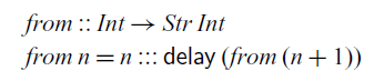
This definition translates to the $\lambda_{\checkmark\!\!\checkmark}$
term
$\lambda_{\checkmark\!\!\checkmark}$
term $\mathsf{fix}\, r. \lambda n. n ::: \mathsf{delay} (\mathsf{adv}\, (\mathsf{unbox}\, r)\, (n+\bar{1}))$
, which, in turn, rewrites into the following
$\mathsf{fix}\, r. \lambda n. n ::: \mathsf{delay} (\mathsf{adv}\, (\mathsf{unbox}\, r)\, (n+\bar{1}))$
, which, in turn, rewrites into the following $\lambda_{\checkmark}$
term:
$\lambda_{\checkmark}$
term:
 \begin{equation*}
\mathit{from} = \mathsf{fix}\, r. \lambda n. n ::: {\rm let}{r'}{\mathsf{unbox}\, r}{\mathsf{delay} (\mathsf{adv}\, r'\, (n+\bar{1}))}
\end{equation*}
\begin{equation*}
\mathit{from} = \mathsf{fix}\, r. \lambda n. n ::: {\rm let}{r'}{\mathsf{unbox}\, r}{\mathsf{delay} (\mathsf{adv}\, r'\, (n+\bar{1}))}
\end{equation*}
Let’s see how the term $\mathit{from}\,\bar{0}$
of type
$\mathit{from}\,\bar{0}$
of type ${\textit{Str}\;\textit{Int}}$
is executed on the machine:
${\textit{Str}\;\textit{Int}}$
is executed on the machine:
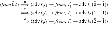 \begin{equation*}
\begin{array}{rcl}
\langle{\mathit{from}\,\bar{0}}{\emptyset}\rangle
&\overset{\bar{0}}{\Longrightarrow}& {\langle\mathsf{adv}\,l'_1}{l_1} \mapsto
\textit{from},\,l'_1\mapsto \mathsf{adv}\,l_1\,(\bar{0} +
\bar{1})\rangle\\
&\overset{\bar{1}}{\Longrightarrow}& \langle\mathsf{adv}\,l'_2{l_2} \mapsto
\textit{from},\,l'_2\mapsto \mathsf{adv}\,l_2\, (\bar{1} + \bar{1})\rangle\\
&\overset{\bar{2}}{\Longrightarrow}& \langle\mathsf{adv}\,l'_3{l_3} \mapsto
\textit{from},\,l'_3\mapsto \mathsf{adv}\,l_3\,(\bar{2} + \bar{1})\rangle\\
&\vdots&
\end{array}
\end{equation*}
\begin{equation*}
\begin{array}{rcl}
\langle{\mathit{from}\,\bar{0}}{\emptyset}\rangle
&\overset{\bar{0}}{\Longrightarrow}& {\langle\mathsf{adv}\,l'_1}{l_1} \mapsto
\textit{from},\,l'_1\mapsto \mathsf{adv}\,l_1\,(\bar{0} +
\bar{1})\rangle\\
&\overset{\bar{1}}{\Longrightarrow}& \langle\mathsf{adv}\,l'_2{l_2} \mapsto
\textit{from},\,l'_2\mapsto \mathsf{adv}\,l_2\, (\bar{1} + \bar{1})\rangle\\
&\overset{\bar{2}}{\Longrightarrow}& \langle\mathsf{adv}\,l'_3{l_3} \mapsto
\textit{from},\,l'_3\mapsto \mathsf{adv}\,l_3\,(\bar{2} + \bar{1})\rangle\\
&\vdots&
\end{array}
\end{equation*}
In each step, the heap contains at location $l_i$
the fixed point
$l_i$
the fixed point $\mathit{from}$
and at location
$\mathit{from}$
and at location $l'_i$
the delayed computation produced by the occurrence of
$l'_i$
the delayed computation produced by the occurrence of $\mathsf{delay}$
in the body of the fixed point. The old versions of the delayed computations are garbage collected after each step and only the most recent version survives.
$\mathsf{delay}$
in the body of the fixed point. The old versions of the delayed computations are garbage collected after each step and only the most recent version survives.
Our main result is that the execution of $\lambda_{\checkmark}$
terms by the machine described in Figure 6 and 7 is safe. To describe the type of the produced values precisely, we need to restrict ourselves to streams over types whose evaluation is not suspended, which excludes function and modal types. This idea is expressed in the notion of value types, defined by the following grammar:
$\lambda_{\checkmark}$
terms by the machine described in Figure 6 and 7 is safe. To describe the type of the produced values precisely, we need to restrict ourselves to streams over types whose evaluation is not suspended, which excludes function and modal types. This idea is expressed in the notion of value types, defined by the following grammar:
 \begin{equation*}
\text{Value types} \quad V, W::= 1\mid{\rm Int} \mid U
\times W \mid U + W
\end{equation*}
\begin{equation*}
\text{Value types} \quad V, W::= 1\mid{\rm Int} \mid U
\times W \mid U + W
\end{equation*}
We can then prove the following theorem, which both expresses the fact that the aggressive garbage collection strategy of $\mathsf{Rattus}$
is safe, and that stream programs are productive:
$\mathsf{Rattus}$
is safe, and that stream programs are productive:
Theorem 4.2
(productivity of streams) Given a term $\vdash_{\checkmark}{t}:{\mathsf{Str}\, A}$
with A a value type, there is an infinite reduction sequence
$\vdash_{\checkmark}{t}:{\mathsf{Str}\, A}$
with A a value type, there is an infinite reduction sequence
 \begin{equation*}
\langle{t};{\emptyset}\rangle {\overset {v_0}\Longrightarrow}
\langle{t_1};{\eta_1}
{\overset{v_1}\Longrightarrow} \langle{t_2}:{\eta_2}\rangle
{\overset{v_2}\Longrightarrow} \ldots \qquad \text{such that}
\vdash_{\checkmark}{v_i}:{A} for all i \ge 0.
\end{equation*}
\begin{equation*}
\langle{t};{\emptyset}\rangle {\overset {v_0}\Longrightarrow}
\langle{t_1};{\eta_1}
{\overset{v_1}\Longrightarrow} \langle{t_2}:{\eta_2}\rangle
{\overset{v_2}\Longrightarrow} \ldots \qquad \text{such that}
\vdash_{\checkmark}{v_i}:{A} for all i \ge 0.
\end{equation*}
The restriction to value types is only necessary for showing that each output value $v_i$
has the correct type.
$v_i$
has the correct type.
4.3.2 Productivity and causality of stream transducers
The step semantics ${\overset {vv'}\Longrightarrow}$
from Figure 7 describes how a term of type
${\overset {vv'}\Longrightarrow}$
from Figure 7 describes how a term of type ${\textit{Str}\;\textit{A}\to \textit{Str}\;\textit{B}}$
transforms a stream of inputs into a stream of outputs in a step-by-step fashion. Given a closed term
${\textit{Str}\;\textit{A}\to \textit{Str}\;\textit{B}}$
transforms a stream of inputs into a stream of outputs in a step-by-step fashion. Given a closed term $\vdash_{\!\checkmark}{t}:\mathsf{Str}\,A\to \mathsf{Str}\,B$
and an infinite stream of input values
$\vdash_{\!\checkmark}{t}:\mathsf{Str}\,A\to \mathsf{Str}\,B$
and an infinite stream of input values $\vdash_{\!\checkmark}{v}_{i}:A$
, it produces an infinite reduction sequence
$\vdash_{\!\checkmark}{v}_{i}:A$
, it produces an infinite reduction sequence
 \begin{equation*}
\langle{t\,(\mathsf{adv}\,l^\ast)};{\emptyset}\rangle
{\overset ({v_0}/{v'_0}\Longrightarrow} \langle{t_1};{\eta_1}\rangle
{\overset ({v_1}/{v'_1}\Longrightarrow}\langle{t_2};{\eta_2}\rangle
{\overset ({v_2}/{v'_1}\Longrightarrow} \ldots
\end{equation*}
\begin{equation*}
\langle{t\,(\mathsf{adv}\,l^\ast)};{\emptyset}\rangle
{\overset ({v_0}/{v'_0}\Longrightarrow} \langle{t_1};{\eta_1}\rangle
{\overset ({v_1}/{v'_1}\Longrightarrow}\langle{t_2};{\eta_2}\rangle
{\overset ({v_2}/{v'_1}\Longrightarrow} \ldots
\end{equation*}
where each output value $v'_i$
has type B.
$v'_i$
has type B.
The definition of ${\overset {vv'}\Longrightarrow}$
assumes that we have some fixed heap location
${\overset {vv'}\Longrightarrow}$
assumes that we have some fixed heap location $l^\ast$
, which acts both as interface to the currently available input value and as a stand-in for future inputs that are not yet available. As we can see above, this stand-in value
$l^\ast$
, which acts both as interface to the currently available input value and as a stand-in for future inputs that are not yet available. As we can see above, this stand-in value $l^\ast$
is passed on to the stream function in the form of the argument
$l^\ast$
is passed on to the stream function in the form of the argument $\mathsf{adv}\,l^\ast$
. Then, in each step, we evaluate the current term
$\mathsf{adv}\,l^\ast$
. Then, in each step, we evaluate the current term $t_i$
in the current heap
$t_i$
in the current heap $\eta_i$
:
$\eta_i$
:
 \begin{equation*}
{t_i}{\eta_i,l^\ast \mapsto v_i ::: l^\ast \checkmark l^\ast
\mapsto \langle\rangle}{v'_i ::: l}{\eta'_i\checkmark\eta_{i+1},l^\ast
\mapsto \langle\rangle}
\end{equation*}
\begin{equation*}
{t_i}{\eta_i,l^\ast \mapsto v_i ::: l^\ast \checkmark l^\ast
\mapsto \langle\rangle}{v'_i ::: l}{\eta'_i\checkmark\eta_{i+1},l^\ast
\mapsto \langle\rangle}
\end{equation*}
which produces the output $v'_i$
and the new heap
$v'_i$
and the new heap $\eta_{i+1}$
. Again the old heap
$\eta_{i+1}$
. Again the old heap $\eta'_i$
is simply dropped. In the ‘later’ heap, the operational semantics maps
$\eta'_i$
is simply dropped. In the ‘later’ heap, the operational semantics maps $l^\ast$
to the placeholder value
$l^\ast$
to the placeholder value $\langle\rangle$
, which is safe since the machine never reads from the ‘later’ heap. Then in the next reduction step, we replace that placeholder value with
$\langle\rangle$
, which is safe since the machine never reads from the ‘later’ heap. Then in the next reduction step, we replace that placeholder value with $v_{i+1} ::: l^\ast$
which contains the newly received input value
$v_{i+1} ::: l^\ast$
which contains the newly received input value $v_{i+1}$
.
$v_{i+1}$
.
For an example, consider the following function that takes a stream of integers and produces the stream of prefix sums:
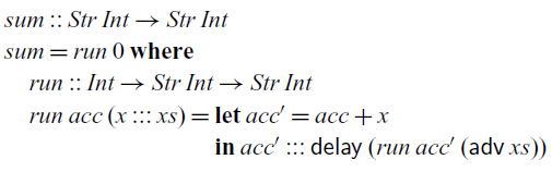
This function definition translates to the following term $\mathit{sum}$
in the
$\mathit{sum}$
in the $\lambda_{\checkmark}$
calculus:
$\lambda_{\checkmark}$
calculus:
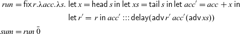 \begin{align*}
\mathit{run} &= \mathsf{fix}\,r.\lambda acc. \lambda s.
\begin{aligned}[t]
&\mathsf{let}\, x = \mathsf{head}\,s \;\mathsf{in}\;
\mathsf{let}\, xs = \mathsf{tail}\,s \;\mathsf{in}\;\mathsf{let}\, acc' = acc + x\; \mathsf{in}\\
&\mathsf{let}\, r' = \,r\; \mathsf{in}\; acc' ::: \mathsf{delay} (\mathsf{adv}\,
r'\, acc' (\mathsf{adv}\, xs))
\end{aligned}
\\
\mathit{sum} &= \mathit{run}\, \bar{0}
\end{align*}
\begin{align*}
\mathit{run} &= \mathsf{fix}\,r.\lambda acc. \lambda s.
\begin{aligned}[t]
&\mathsf{let}\, x = \mathsf{head}\,s \;\mathsf{in}\;
\mathsf{let}\, xs = \mathsf{tail}\,s \;\mathsf{in}\;\mathsf{let}\, acc' = acc + x\; \mathsf{in}\\
&\mathsf{let}\, r' = \,r\; \mathsf{in}\; acc' ::: \mathsf{delay} (\mathsf{adv}\,
r'\, acc' (\mathsf{adv}\, xs))
\end{aligned}
\\
\mathit{sum} &= \mathit{run}\, \bar{0}
\end{align*}
Let’s look at the first three steps of executing the $\mathit{sum}$
function with 2, 11 and 5 as its first three input values:
$\mathit{sum}$
function with 2, 11 and 5 as its first three input values:
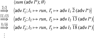
In each step of the computation, $l_i$
stores the fixed point
$l_i$
stores the fixed point $\textit{run}$
and
$\textit{run}$
and $l'_i$
stores the computation that calls that fixed point with the new accumulator value (2, 13 and 18, respectively) and the tail of the current input stream.
$l'_i$
stores the computation that calls that fixed point with the new accumulator value (2, 13 and 18, respectively) and the tail of the current input stream.
We can prove the following theorem, which again expresses the fact that the garbage collection strategy of $\mathsf{Rattus}$
is safe, and that stream processing functions are both productive and causal:
$\mathsf{Rattus}$
is safe, and that stream processing functions are both productive and causal:
Theorem 4.3 (causality and productivity of stream transducers) Given a term $\vdash_{\!\!\checkmark}t:{\mathsf{Str}\, A \to \mathsf{Str}\, B}$
with B a value type, and an infinite sequence of values
$\vdash_{\!\!\checkmark}t:{\mathsf{Str}\, A \to \mathsf{Str}\, B}$
with B a value type, and an infinite sequence of values $\vdash_{\!\!\checkmark}v_i:A$
, there is an infinite reduction sequence
$\vdash_{\!\!\checkmark}v_i:A$
, there is an infinite reduction sequence
Since the operational semantics is deterministic, in each step
 $\langle{t_i};{\eta_i}\rangle \overset{v_{i}/v'_{i}}\Longrightarrow
\langle{t_{i+1}};{\eta_{i+1}}\rangle$
, the resulting output
$\langle{t_i};{\eta_i}\rangle \overset{v_{i}/v'_{i}}\Longrightarrow
\langle{t_{i+1}};{\eta_{i+1}}\rangle$
, the resulting output $v'_{i+1}$
and new state of the computation
$v'_{i+1}$
and new state of the computation $\langle{t_{i+1}};{\eta_{i+1}}\rangle$
are uniquely determined by the previous state
$\langle{t_{i+1}};{\eta_{i+1}}\rangle$
are uniquely determined by the previous state $\langle{t_i};{\eta_i}\rangle$
and the input
$\langle{t_i};{\eta_i}\rangle$
and the input $v_{i}$
. Thus,
$v_{i}$
. Thus, $v'_{i}$
and
$v'_{i}$
and $\langle{t_{i+1}};{\eta_{i+1}}\rangle$
are independent of future inputs
$\langle{t_{i+1}};{\eta_{i+1}}\rangle$
are independent of future inputs $v_j$
with
$v_j$
with $j > i$
.
$j > i$
.
4.3.3 Space leak in the naive operational semantics
Theorems 4.2 and 4.3 show that $\lambda_{\checkmark\!\!\checkmark}$
terms can be executed without implicit space leaks after they have been translated into
$\lambda_{\checkmark\!\!\checkmark}$
terms can be executed without implicit space leaks after they have been translated into $\lambda_{\checkmark}$
terms. To demonstrate the need of the translation step, we give an example that illustrates what would happen if we would skip it.
$\lambda_{\checkmark}$
terms. To demonstrate the need of the translation step, we give an example that illustrates what would happen if we would skip it.
Since both $\lambda_{\checkmark}$
and
$\lambda_{\checkmark}$
and $\lambda_{\checkmark\!\!\checkmark}$
share the same syntax, the abstract machine from Section 4.2.2 could in principle be used for
$\lambda_{\checkmark\!\!\checkmark}$
share the same syntax, the abstract machine from Section 4.2.2 could in principle be used for $\lambda_{\checkmark\!\!\checkmark}$
terms directly, without transforming them to
$\lambda_{\checkmark\!\!\checkmark}$
terms directly, without transforming them to $\lambda_{\checkmark}$
first. However, we can construct a well-typed
$\lambda_{\checkmark}$
first. However, we can construct a well-typed $\lambda_{\checkmark\!\!\checkmark}$
term for which the machine will try to dereference a heap location that has previously been garbage collected. We might conjecture that we could accommodate direct execution of
$\lambda_{\checkmark\!\!\checkmark}$
term for which the machine will try to dereference a heap location that has previously been garbage collected. We might conjecture that we could accommodate direct execution of $\lambda_{\checkmark\!\!\checkmark}$
by increasing the number of available heaps in the abstract machine so that it matches the number of ticks that were necessary to type-check the term we wish to execute. But this is not the case: we can construct a
$\lambda_{\checkmark\!\!\checkmark}$
by increasing the number of available heaps in the abstract machine so that it matches the number of ticks that were necessary to type-check the term we wish to execute. But this is not the case: we can construct a $\lambda_{\checkmark\!\!\checkmark}$
term that can be type-checked with only two ticks but requires an unbounded number of heaps to safely execute directly. In other words, programs in
$\lambda_{\checkmark\!\!\checkmark}$
term that can be type-checked with only two ticks but requires an unbounded number of heaps to safely execute directly. In other words, programs in $\lambda_{\checkmark\!\!\checkmark}$
may exhibit implicit space leaks, if we just run them using the evaluation strategy of the abstract machine from Section 4.2.2.
$\lambda_{\checkmark\!\!\checkmark}$
may exhibit implicit space leaks, if we just run them using the evaluation strategy of the abstract machine from Section 4.2.2.
Such implicit space leaks can occur in $\lambda_{\checkmark\!\!\checkmark}$
for two reasons: (1) a lambda abstraction that appears in the scope of a
$\lambda_{\checkmark\!\!\checkmark}$
for two reasons: (1) a lambda abstraction that appears in the scope of a $\checkmark$
, and (2) a term that requires more than one
$\checkmark$
, and (2) a term that requires more than one $\checkmark$
to type-check. Bahr et al. (Reference Bahr, Graulund and Møgelberg2019) give an example of (1), which translates to
$\checkmark$
to type-check. Bahr et al. (Reference Bahr, Graulund and Møgelberg2019) give an example of (1), which translates to $\lambda_{\checkmark\!\!\checkmark}$
. The following term of type
$\lambda_{\checkmark\!\!\checkmark}$
. The following term of type $\bigcirc (\mathsf{Str}\, Int) \to \bigcirc (\mathsf{Str}\, Int)$
is an example of (2):
$\bigcirc (\mathsf{Str}\, Int) \to \bigcirc (\mathsf{Str}\, Int)$
is an example of (2):
 \begin{equation*}
t = \mathsf{fix}\,r.\lambda x. \mathsf{delay} (head (\mathsf{adv}\, x) ::: \mathsf{adv}(\mathsf{unbox}\, r) (\mathsf{delay} (\mathsf{adv} (tail (\mathsf{adv}\, x)))))
\end{equation*}
\begin{equation*}
t = \mathsf{fix}\,r.\lambda x. \mathsf{delay} (head (\mathsf{adv}\, x) ::: \mathsf{adv}(\mathsf{unbox}\, r) (\mathsf{delay} (\mathsf{adv} (tail (\mathsf{adv}\, x)))))
\end{equation*}
The abstract machine would get stuck trying to dereference a heap location that was previously garbage collected. The problem is that the second occurrence of x is nested below two occurrences of $\mathsf{delay}$
. As a consequence, when
$\mathsf{delay}$
. As a consequence, when $\mathsf{adv}\,x$
is evaluated, the heap location bound to x is two time steps old and has been garbage collected already.
$\mathsf{adv}\,x$
is evaluated, the heap location bound to x is two time steps old and has been garbage collected already.
To see this behaviour on a concrete example, recall the $\lambda_{\checkmark}$
term
$\lambda_{\checkmark}$
term $\mathit{from} : Int \to \mathsf{Str}\, Int$
from Section 4.3.1, which produces a stream of consecutive integers. Using t and
$\mathit{from} : Int \to \mathsf{Str}\, Int$
from Section 4.3.1, which produces a stream of consecutive integers. Using t and $\mathit{from}$
, we can construct the
$\mathit{from}$
, we can construct the $\lambda_{\checkmark\!\!\checkmark}$
term
$\lambda_{\checkmark\!\!\checkmark}$
term $\bar{0} ::: t\, (\mathsf{delay}\,(\mathit{from}\,\bar{1}))$
of type
$\bar{0} ::: t\, (\mathsf{delay}\,(\mathit{from}\,\bar{1}))$
of type $\mathsf{Str}\, Int$
, which we can run on the abstract machine:
Footnote 6
$\mathsf{Str}\, Int$
, which we can run on the abstract machine:
Footnote 6
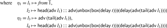
In the last step, the machine would get stuck trying to evaluate $\mathsf{adv}\,l_4$
, since this in turn requires evaluating
$\mathsf{adv}\,l_4$
, since this in turn requires evaluating $\mathsf{head} (\mathsf{adv}\, l_3)$
and
$\mathsf{head} (\mathsf{adv}\, l_3)$
and $\mathsf{adv}\,(\mathsf{tail}(\mathsf{adv}\,l_1))$
, which would require looking up
$\mathsf{adv}\,(\mathsf{tail}(\mathsf{adv}\,l_1))$
, which would require looking up $l_1$
in
$l_1$
in $\eta_1$
, which has already been garbage collected. Assuming we modified the machine so that it does not perform garbage collection, but instead holds on to the previous heaps
$\eta_1$
, which has already been garbage collected. Assuming we modified the machine so that it does not perform garbage collection, but instead holds on to the previous heaps $\eta_1,\eta_2$
, it would continue as follows:
$\eta_1,\eta_2$
, it would continue as follows:
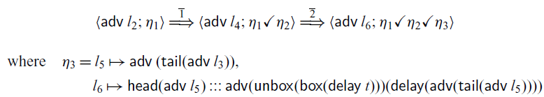
The next execution step would require the machine to look up $l_6$
, which in turn requires
$l_6$
, which in turn requires $l_5$
,
$l_5$
, $l_3$
, and eventually
$l_3$
, and eventually $l_1$
. We could continue this arbitrarily far into the future, and in each step the machine would need to look up
$l_1$
. We could continue this arbitrarily far into the future, and in each step the machine would need to look up $l_1$
in the very first heap
$l_1$
in the very first heap $\eta_1$
.
$\eta_1$
.
This examples suggests that the cause of this space leak is the fact that the machine leaves the nested terms $\mathsf{adv}\, l_1$
,
$\mathsf{adv}\, l_1$
, $\mathsf{adv}\, l_3$
, etc. unevaluated on the heap. As our metatheoretical results in this section show, the translation into
$\mathsf{adv}\, l_3$
, etc. unevaluated on the heap. As our metatheoretical results in this section show, the translation into $\lambda_{\checkmark}$
avoids this problem. Indeed, if we apply the rewrite rules from Section 4.2.1 to t, we obtain the
$\lambda_{\checkmark}$
avoids this problem. Indeed, if we apply the rewrite rules from Section 4.2.1 to t, we obtain the $\lambda_{\checkmark}$
term
$\lambda_{\checkmark}$
term
 $\overline 0 ::: t' \,
(\mathsf{delay}\,(\mathit{from}\,\overline 1))$
, where
$\overline 0 ::: t' \,
(\mathsf{delay}\,(\mathit{from}\,\overline 1))$
, where
This term can then be safely executed on the abstract machine:
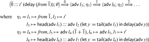
4.4 Limitations
Now that we have formally precise statements about the operational properties of $\mathsf{Rattus}$
’ core calculus, we should make sure that we understand what they mean in practice and what their limitations are. In simple terms, the productivity and causality properties established by Theorems 4.2 and 4.3 state that reactive programs in
$\mathsf{Rattus}$
’ core calculus, we should make sure that we understand what they mean in practice and what their limitations are. In simple terms, the productivity and causality properties established by Theorems 4.2 and 4.3 state that reactive programs in $\mathsf{Rattus}$
can be executed effectively – they always make progress and never depend on data that is not yet available. However,
$\mathsf{Rattus}$
can be executed effectively – they always make progress and never depend on data that is not yet available. However, $\mathsf{Rattus}$
allows calling general Haskell functions, for which we can make no such operational guarantees. This trade-off is intentional as we wish to make Haskell’s rich library ecosystem available to
$\mathsf{Rattus}$
allows calling general Haskell functions, for which we can make no such operational guarantees. This trade-off is intentional as we wish to make Haskell’s rich library ecosystem available to $\mathsf{Rattus}$
. Similar trade-offs are common in foreign function interfaces that allow function calls into another language. For instance, Haskell code may call C functions.
$\mathsf{Rattus}$
. Similar trade-offs are common in foreign function interfaces that allow function calls into another language. For instance, Haskell code may call C functions.
In addition, by virtue of the operational semantics, Theorems 4.2 and 4.3 also imply that programs can be executed without implicitly retaining memory – thus avoiding implicit space leaks. This follows from the fact that in each step, the step semantics (cf. Figure 7) discards the ‘now’ heap and only retains the ‘later’ heap for the next step. However, similarly to the calculi of Krishnaswami (Reference Krishnaswami2013) and Bahr et al. (Reference Bahr, Graulund and Møgelberg2021, Reference Bahr, Graulund and Møgelberg2019), $\mathsf{Rattus}$
still allows explicit space leaks (we may still construct data structures to hold on to an increasing amount of memory) as well as time leaks (computations may take an increasing amount of time). Below we give some examples of these behaviours.
$\mathsf{Rattus}$
still allows explicit space leaks (we may still construct data structures to hold on to an increasing amount of memory) as well as time leaks (computations may take an increasing amount of time). Below we give some examples of these behaviours.
Given a strict list type List (cf. Section 3.2), we can construct a function that buffers the entire history of its input stream:
Given that we have a function sum :: List Int → Int that computes the sum of a list of numbers, we can write the following alternative implementation of the sums function using buffer:
At each time step, this function adds the current input integer to the buffer of type List Int and then computes the sum of the current value of that buffer. This function exhibits both a space leak (buffering a steadily growing list of numbers) and a time leak (the time to compute each element of the resulting stream increases at each step). However, these leaks are explicit in the program.
An example of a time leak is found in the following alternative implementation of the sums function:
In each step, we add the current input value x to each future output. The closure ${(+x)}$
, which is Haskell shorthand notation for
${(+x)}$
, which is Haskell shorthand notation for $\lambda y \to y + x$
, stores each input value x.
$\lambda y \to y + x$
, stores each input value x.
None of the above space and time leaks are prevented by $\mathsf{Rattus}$
. The space leaks in
$\mathsf{Rattus}$
. The space leaks in ${\textit{buffer}}$
and
${\textit{buffer}}$
and ${\textit{leakySums1}}$
are explicit, since the desire to buffer the input is explicitly stated in the program. That is, while
${\textit{leakySums1}}$
are explicit, since the desire to buffer the input is explicitly stated in the program. That is, while $\mathsf{Rattus}$
prevents implicit space leaks, it still allows programmers to allocate memory as they see fit. The other example is more subtle as the leaky behaviour is rooted in a time leak as the program constructs an increasing computation in each step. This shows that the programmer still has to be careful about time leaks. Note that these leaky functions can also be implemented in the calculi of Krishnaswami (Reference Krishnaswami2013) and Bahr et al. (Reference Bahr, Graulund and Møgelberg2019, Reference Bahr, Graulund and Møgelberg2021), although some reformulation is necessary for the Simply RaTT calculus of Bahr et al. (Reference Bahr, Graulund and Møgelberg2019).
$\mathsf{Rattus}$
prevents implicit space leaks, it still allows programmers to allocate memory as they see fit. The other example is more subtle as the leaky behaviour is rooted in a time leak as the program constructs an increasing computation in each step. This shows that the programmer still has to be careful about time leaks. Note that these leaky functions can also be implemented in the calculi of Krishnaswami (Reference Krishnaswami2013) and Bahr et al. (Reference Bahr, Graulund and Møgelberg2019, Reference Bahr, Graulund and Møgelberg2021), although some reformulation is necessary for the Simply RaTT calculus of Bahr et al. (Reference Bahr, Graulund and Møgelberg2019).
4.5 Language design considerations
The design of $\mathsf{Rattus}$
and its core calculus is derived from the calculi of Krishnaswami (Reference Krishnaswami2013) and Bahr et al. (Reference Bahr, Graulund and Møgelberg2019, Reference Bahr, Graulund and Møgelberg2021), which are the only other modal FRP calculi with a garbage collection result similar to ours. In the following, we review the differences of
$\mathsf{Rattus}$
and its core calculus is derived from the calculi of Krishnaswami (Reference Krishnaswami2013) and Bahr et al. (Reference Bahr, Graulund and Møgelberg2019, Reference Bahr, Graulund and Møgelberg2021), which are the only other modal FRP calculi with a garbage collection result similar to ours. In the following, we review the differences of $\mathsf{Rattus}$
compared to these calculi with the aim of illustrating how the design of
$\mathsf{Rattus}$
compared to these calculi with the aim of illustrating how the design of $\mathsf{Rattus}$
follows from our goal to simplify previous calculi while still maintaining their strong operational properties.
$\mathsf{Rattus}$
follows from our goal to simplify previous calculi while still maintaining their strong operational properties.
Like the present work, the Simply RaTT calculus of Bahr et al. (Reference Bahr, Graulund and Møgelberg2019) uses a Fitch-style type system, which provides lighter syntax to interact with the $\square$
and
$\square$
and $\bigcirc$
modality compared to Krishnaswami’s use of qualifiers in his calculus. In addition, Simply RaTT also dispenses with the allocation tokens of Krishnaswami’s calculus by making the
$\bigcirc$
modality compared to Krishnaswami’s use of qualifiers in his calculus. In addition, Simply RaTT also dispenses with the allocation tokens of Krishnaswami’s calculus by making the $\mathsf{box}$
primitive call-by-name. By contrast, Krishnaswami’s calculus is closely related to dual-context systems and requires the use of pattern matching as elimination forms of the modalities. The Lively RaTT calculus of Bahr et al. (Reference Bahr, Graulund and Møgelberg2021) extends Simply RaTT with temporal inductive types to express liveness properties. But otherwise, Lively RaTT is similar to Simply RaTT and the discussion below equally applies to Lively RaTT as well.
$\mathsf{box}$
primitive call-by-name. By contrast, Krishnaswami’s calculus is closely related to dual-context systems and requires the use of pattern matching as elimination forms of the modalities. The Lively RaTT calculus of Bahr et al. (Reference Bahr, Graulund and Møgelberg2021) extends Simply RaTT with temporal inductive types to express liveness properties. But otherwise, Lively RaTT is similar to Simply RaTT and the discussion below equally applies to Lively RaTT as well.
As discussed in Section 2.2, Simply RaTT restricts where ticks may occur, which disallows terms like $\mathsf{delay}(\mathsf{delay}\, 0)$
and
$\mathsf{delay}(\mathsf{delay}\, 0)$
and $\mathsf{delay}(\lambda x. x)$
. In addition, Simply RaTT has a more complicated typing rule for guarded fixed points (cf. Figure 8). In addition to
$\mathsf{delay}(\lambda x. x)$
. In addition, Simply RaTT has a more complicated typing rule for guarded fixed points (cf. Figure 8). In addition to $\checkmark$
, Simply RaTT uses the token
$\checkmark$
, Simply RaTT uses the token
![]() to serve the role that stabilisation of a context
to serve the role that stabilisation of a context $\Gamma$
to
$\Gamma$
to $\Gamma^\square$
serves in
$\Gamma^\square$
serves in $\mathsf{Rattus}$
. But Simply RaTT only allows one such
$\mathsf{Rattus}$
. But Simply RaTT only allows one such
![]() token, and
token, and $\checkmark$
may only appear to the right of
$\checkmark$
may only appear to the right of
![]() . Moreover, fixed points in Simply RaTT produce terms of type
. Moreover, fixed points in Simply RaTT produce terms of type $\square A$
rather than just A. Taken together, this makes the syntax and typing for guarded recursive function definitions more complicated and less intuitive. For example, the
$\square A$
rather than just A. Taken together, this makes the syntax and typing for guarded recursive function definitions more complicated and less intuitive. For example, the $\textit{map}$
function would be defined as follows in Simply RaTT:
$\textit{map}$
function would be defined as follows in Simply RaTT:
Fig. 8. Selected typing rules from Bahr et al. (Reference Bahr, Graulund and Møgelberg2019).
Here, # is used to indicate that the argument f is to the left of the
![]() token and only because of the presence of this token can we use the
token and only because of the presence of this token can we use the $\mathsf{unbox}$
combinator on f (cf. Figure 8). Additionally, the typing of recursive definitions is somewhat confusing:
$\mathsf{unbox}$
combinator on f (cf. Figure 8). Additionally, the typing of recursive definitions is somewhat confusing: $\textit{map}$
has return type
$\textit{map}$
has return type ![]() (str a → str b) but when used in a recursive call as seen above, map f is of type ○(str a → str b) instead. Moreover, we cannot call
(str a → str b) but when used in a recursive call as seen above, map f is of type ○(str a → str b) instead. Moreover, we cannot call $\textit{map}$
recursively on its own. All recursive calls must be of the form map f, the exact pattern that appears to the left of the #. This last restriction rules out the following variant of
$\textit{map}$
recursively on its own. All recursive calls must be of the form map f, the exact pattern that appears to the left of the #. This last restriction rules out the following variant of $\textit{map}$
that is meant to take two functions and alternately apply them to a stream:
$\textit{map}$
that is meant to take two functions and alternately apply them to a stream:
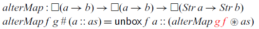
Only alter Map f g is allowed as recursive call, but not alter Map g f. By contrast, alter Map can be implemented in $\mathsf{Rattus}$
without problems:
$\mathsf{Rattus}$
without problems:
In addition, because guarded recursive functions always have a boxed return type, definitions in Simply RaTT are often littered with calls to $\mathsf{unbox}$
. For example, the function pong
1 from Section 3.2 would be implemented as follows in Simply RaTT:
$\mathsf{unbox}$
. For example, the function pong
1 from Section 3.2 would be implemented as follows in Simply RaTT:
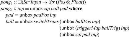
By making the type of guarded fixed points A rather than $\square A$
, we avoid all of the above issues related to guarded recursive definitions. Moreover, the unrestricted
$\square A$
, we avoid all of the above issues related to guarded recursive definitions. Moreover, the unrestricted $\mathsf{unbox}$
combinator found in
$\mathsf{unbox}$
combinator found in $\mathsf{Rattus}$
follows directly from this change in the guarded fixed point typing. If we were to change the typing rule for
$\mathsf{Rattus}$
follows directly from this change in the guarded fixed point typing. If we were to change the typing rule for $\mathsf{fix}$
in Simply RaTT so that
$\mathsf{fix}$
in Simply RaTT so that $\mathsf{fix}$
has type A instead of
$\mathsf{fix}$
has type A instead of $\square A$
, we would be able to define an unrestricted
$\square A$
, we would be able to define an unrestricted $\mathsf{unbox}$
combinator
$\mathsf{unbox}$
combinator $\lambda x. \mathsf{fix}\, y.\mathsf{unbox}\, x$
of type
$\lambda x. \mathsf{fix}\, y.\mathsf{unbox}\, x$
of type $\square A \to A$
.
$\square A \to A$
.
Conversely, if we keep the $\mathsf{unbox}$
combinator of Simply RaTT but lift some of the restrictions regarding the
$\mathsf{unbox}$
combinator of Simply RaTT but lift some of the restrictions regarding the
![]() token such as allowing
token such as allowing $\checkmark$
not only to the right of a
$\checkmark$
not only to the right of a
![]() or allowing more than one
or allowing more than one
![]() token, then we would break the garbage collection property and thus permit leaky programs. In such a modified version of Simply RaTT, we would be able to type-check the following term:
token, then we would break the garbage collection property and thus permit leaky programs. In such a modified version of Simply RaTT, we would be able to type-check the following term:
where $\Gamma = \sharp$
if we were to allow two
$\Gamma = \sharp$
if we were to allow two
![]() tokens or
tokens or $\Gamma$
empty, if we were to allow the
$\Gamma$
empty, if we were to allow the $\checkmark$
to occur left of the
$\checkmark$
to occur left of the
![]() . The above term stores the value
. The above term stores the value $\mathsf{box}\,0$
on the heap and then constructs a stream, which at each step tries to read this value from the heap location. Hence, in order to maintain the garbage collection property in
$\mathsf{box}\,0$
on the heap and then constructs a stream, which at each step tries to read this value from the heap location. Hence, in order to maintain the garbage collection property in $\mathsf{Rattus}$
, we had to change the typing rule for
$\mathsf{Rattus}$
, we had to change the typing rule for $\mathsf{unbox}$
.
$\mathsf{unbox}$
.
In addition, $\mathsf{Rattus}$
permits recursive functions that look more than one time step into the future (e.g.,
$\mathsf{Rattus}$
permits recursive functions that look more than one time step into the future (e.g., $\textit{stutter}$
from Section 2.2), which is not possible in Krishnaswami (Reference Krishnaswami2013) and Bahr et al. (Reference Bahr, Graulund and Møgelberg2019, Reference Bahr, Graulund and Møgelberg2021). However, we conjecture that Krishnaswami’s calculus can be adapted to allow this by changing the typing rule for
$\textit{stutter}$
from Section 2.2), which is not possible in Krishnaswami (Reference Krishnaswami2013) and Bahr et al. (Reference Bahr, Graulund and Møgelberg2019, Reference Bahr, Graulund and Møgelberg2021). However, we conjecture that Krishnaswami’s calculus can be adapted to allow this by changing the typing rule for $\mathsf{fix}$
in a similar way as we did for
$\mathsf{fix}$
in a similar way as we did for $\mathsf{Rattus}$
.
$\mathsf{Rattus}$
.
We should note that that the # token found in Simply RaTT has some benefit over the $\Gamma^\square$
construction. It allows the calculus to reject some programs with time leaks, for example,
$\Gamma^\square$
construction. It allows the calculus to reject some programs with time leaks, for example,
![]() from Section 4.4, because of the condition in the rule for
from Section 4.4, because of the condition in the rule for $\mathsf{unbox}$
requiring that
$\mathsf{unbox}$
requiring that $\Gamma'$
be token-free. However, we can easily write a program that is equivalent to
$\Gamma'$
be token-free. However, we can easily write a program that is equivalent to
![]() , that is well-typed in Simply RaTT using tupling, which corresponds to defining
, that is well-typed in Simply RaTT using tupling, which corresponds to defining
![]() mutually recursively with
mutually recursively with $\textit{map}$
. Moreover, this side condition for
$\textit{map}$
. Moreover, this side condition for $\mathsf{unbox}$
was dropped in Lively RaTT as it is incompatible with the extension by temporal inductive types.
$\mathsf{unbox}$
was dropped in Lively RaTT as it is incompatible with the extension by temporal inductive types.
Finally, there is an interesting trade-off in all four calculi in terms of their syntactic properties such as eta-expansion and local soundness/completeness. The potential lack of these syntactic properties has no bearing on the semantic soundness results for these calculi, but it may be counterintuitive to a programmer using the language.
For example, typing in Simply RaTT is closed under certain eta-expansions involving $\square$
, which are no longer well-typed in
$\square$
, which are no longer well-typed in $\lambda_{\checkmark\!\!\checkmark}$
because of the typing rule for
$\lambda_{\checkmark\!\!\checkmark}$
because of the typing rule for $\mathsf{unbox}$
. For example, we have
$\mathsf{unbox}$
. For example, we have
 \begin{equation*} f : A \to \square B \vdash \lambda\, x. \mathsf{box} (\mathsf{unbox} (f\,x)):A \to \square B \end{equation*}
in Simply RaTT but not in $\lambda_{\checkmark\!\!\checkmark}$
. However,
$\lambda_{\checkmark\!\!\checkmark}$
. However, $\lambda_{\checkmark\!\!\checkmark}$
has a slightly different eta-expansion for this type instead:
$\lambda_{\checkmark\!\!\checkmark}$
has a slightly different eta-expansion for this type instead:
which matches the eta-expansion in Krishnaswami’s calculus:
On the other hand, because $\lambda_{\checkmark\!\!\checkmark}$
lifts Simply RaTT’s restrictions on tokens,
$\lambda_{\checkmark\!\!\checkmark}$
lifts Simply RaTT’s restrictions on tokens, $\lambda_{\checkmark\!\!\checkmark}$
is closed under several types of eta-expansions that are not well-typed in Simply RaTT. For example,
$\lambda_{\checkmark\!\!\checkmark}$
is closed under several types of eta-expansions that are not well-typed in Simply RaTT. For example,
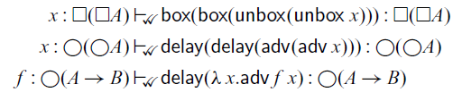
In return, both Krishnaswami’s calculus and $\lambda_{\checkmark\!\!\checkmark}$
lack local soundness and completeness for the
$\lambda_{\checkmark\!\!\checkmark}$
lack local soundness and completeness for the $\square$
type. For instance, from
$\square$
type. For instance, from ${\Gamma}\vdash_{\checkmark\!\!\checkmark}{t}:{\square A}$
we can obtain
${\Gamma}\vdash_{\checkmark\!\!\checkmark}{t}:{\square A}$
we can obtain ${\Gamma}\vdash_{\checkmark\!\!\checkmark}\mathsf{unbox}\, t:A$
in
${\Gamma}\vdash_{\checkmark\!\!\checkmark}\mathsf{unbox}\, t:A$
in $\lambda_{\checkmark\!\!\checkmark}$
, but from
$\lambda_{\checkmark\!\!\checkmark}$
, but from ${\Gamma}\vdash_{\checkmark\!\!\checkmark}{t}:{A}$
, we cannot construct a term
${\Gamma}\vdash_{\checkmark\!\!\checkmark}{t}:{A}$
, we cannot construct a term ${\Gamma}\vdash_{\checkmark\!\!\checkmark}{t'}:{\square A}$
. By contrast, the use of the
${\Gamma}\vdash_{\checkmark\!\!\checkmark}{t'}:{\square A}$
. By contrast, the use of the
![]() token ensures that Simply RaTT enjoys these local soundness and completeness properties. However, Simply RaTT can only allow one such token and must thus trade off eta-expansion as show above in order to avoid space leaks (cf. the example term above).
token ensures that Simply RaTT enjoys these local soundness and completeness properties. However, Simply RaTT can only allow one such token and must thus trade off eta-expansion as show above in order to avoid space leaks (cf. the example term above).
In summary, we argue that our typing system and syntax are simpler than both the work of Krishnaswami (Reference Krishnaswami2013) and Bahr et al. (Reference Bahr, Graulund and Møgelberg2019, Reference Bahr, Graulund and Møgelberg2021). These simplifications are meant to make the language easier to use and integrate more easily with mainstream languages like Haskell, while still maintaining the strong memory guarantees of the earlier calculi.
5 Metatheory
In the previous section, we have presented $\mathsf{Rattus}$
’s core calculus and stated its three central operational properties in Theorems 4.2 and 4.3: productivity, causality, and absence of implicit space leaks. Note that the absence of space leaks follows from these theorems because the operational semantics already ensures this memory property by means of garbage collecting the ‘now’ heap after each step. Since the proof of Theorems 4.2 and 4.3 is fully formalised in the accompanying Coq proofs, we only give a high-level overview of the underlying proof technique here.
$\mathsf{Rattus}$
’s core calculus and stated its three central operational properties in Theorems 4.2 and 4.3: productivity, causality, and absence of implicit space leaks. Note that the absence of space leaks follows from these theorems because the operational semantics already ensures this memory property by means of garbage collecting the ‘now’ heap after each step. Since the proof of Theorems 4.2 and 4.3 is fully formalised in the accompanying Coq proofs, we only give a high-level overview of the underlying proof technique here.
We prove the above-mentioned theorems by establishing a semantic soundness property. For productivity, our soundness property must imply that the evaluation semantics
![]() converges for each well-typed term t, and for causality, the soundness property must imply that this is also the case if t contains references to heap locations in
converges for each well-typed term t, and for causality, the soundness property must imply that this is also the case if t contains references to heap locations in $\sigma$
.
$\sigma$
.
To obtain such a soundness result, we construct a Kripke logical relation that incorporates these properties. Generally speaking, a Kripke logical relation constructs for each type A a relation ${\lbrack\!\,\lbrack A \rbrack\!\,rbrack}_w$
indexed over some world w with some closure conditions when the index w changes. In our case,
${\lbrack\!\,\lbrack A \rbrack\!\,rbrack}_w$
indexed over some world w with some closure conditions when the index w changes. In our case, ${\lbrack\!\,\lbrack A \rbrack\!\,rbrack}_w$
is a set of terms. Moreover, the index w consists of three components: a number
${\lbrack\!\,\lbrack A \rbrack\!\,rbrack}_w$
is a set of terms. Moreover, the index w consists of three components: a number $\nu$
to act as a step index (Appel and McAllester, Reference Appel and McAllester2001), a store
$\nu$
to act as a step index (Appel and McAllester, Reference Appel and McAllester2001), a store $\sigma$
to establish the safety of garbage collection, and an infinite sequence
$\sigma$
to establish the safety of garbage collection, and an infinite sequence $\overline\eta$
of future heaps in order to capture the causality property.
$\overline\eta$
of future heaps in order to capture the causality property.
A crucial ingredient of a Kripke logical relation is the ordering on the indices. The ordering on the number $\nu$
is the standard ordering on numbers. For heaps, we use the standard ordering on partial maps:
$\nu$
is the standard ordering on numbers. For heaps, we use the standard ordering on partial maps: $\eta \sqsubseteq \eta'$
iff
$\eta \sqsubseteq \eta'$
iff $\eta(l) = \eta'(l)$
for all
$\eta(l) = \eta'(l)$
for all $l \in \mathsf{dom}\eta$
. Infinite sequences of heaps are ordered pointwise according to
$l \in \mathsf{dom}\eta$
. Infinite sequences of heaps are ordered pointwise according to $\sqsubseteq$
. Moreover, we extend the ordering to stores in two different ways:
$\sqsubseteq$
. Moreover, we extend the ordering to stores in two different ways:
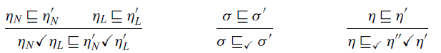
That is,
![]() is the pointwise extension of the order on heaps to stores, whereas
is the pointwise extension of the order on heaps to stores, whereas
![]() is more general and permits introducing an arbitrary ‘now’ heap if none is present.
is more general and permits introducing an arbitrary ‘now’ heap if none is present.
Given these orderings, we define two logical relations, the value relation
![]() and the term relation
and the term relation
![]() . Both are defined in Figure 9 by well-founded recursion according to the lexicographic ordering on the triple
. Both are defined in Figure 9 by well-founded recursion according to the lexicographic ordering on the triple $(\nu,\vert A \vert,e)$
, where
$(\nu,\vert A \vert,e)$
, where $\vert A \vert$
is the size of A defined below, and
$\vert A \vert$
is the size of A defined below, and $e = 1$
for the term relation and
$e = 1$
for the term relation and $e = 0$
for the value relation:
$e = 0$
for the value relation:
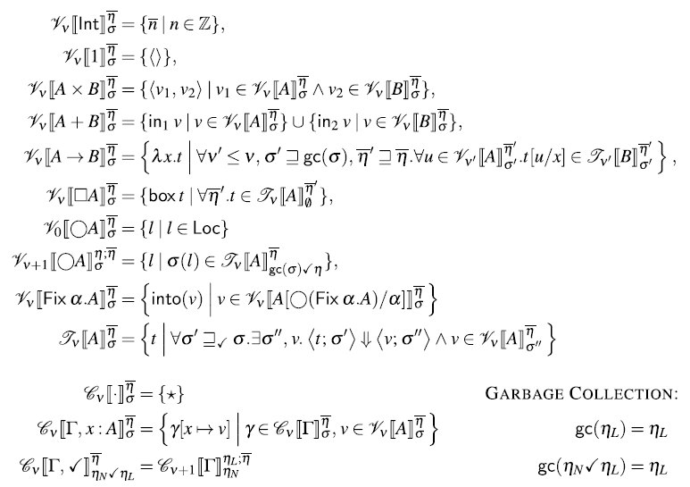
Fig. 9. Logical relation.
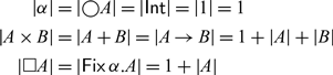
In the definition of the logical relation, we use the notation $\eta;\overline\eta$
to denote an infinite sequence of heaps that starts with the heap
$\eta;\overline\eta$
to denote an infinite sequence of heaps that starts with the heap $\eta$
and then continues as the sequence
$\eta$
and then continues as the sequence $\overline\eta$
. Moreover, we use the notation
$\overline\eta$
. Moreover, we use the notation $\sigma(l)$
to denote
$\sigma(l)$
to denote $\eta_L(l)$
if
$\eta_L(l)$
if $\sigma$
is of the form
$\sigma$
is of the form $\eta_L$
or
$\eta_L$
or $\eta_N\checkmark\eta_L$
.
$\eta_N\checkmark\eta_L$
.
The crucial part of the logical relation that ensures both causality and the absence of space leaks is the case for $\bigcirc A$
. The value relation of
$\bigcirc A$
. The value relation of $\bigcirc A$
at store index
$\bigcirc A$
at store index $\sigma$
is defined as all heap locations that map to computations in the term relation of A but at the store index
$\sigma$
is defined as all heap locations that map to computations in the term relation of A but at the store index $\mathsf{gc}{\sigma}\checkmark\eta$
. Here,
$\mathsf{gc}{\sigma}\checkmark\eta$
. Here, $\mathsf{gc}\sigma$
denotes the garbage collection of the store
$\mathsf{gc}\sigma$
denotes the garbage collection of the store $\sigma$
as defined in Figure 9. It simply drops the ‘now’ heap if present. To see how this definition captures causality, we have to look a the index
$\sigma$
as defined in Figure 9. It simply drops the ‘now’ heap if present. To see how this definition captures causality, we have to look a the index $\eta;\overline\eta$
of future heaps. It changes to the index
$\eta;\overline\eta$
of future heaps. It changes to the index $\overline\eta$
, that is, all future heaps are one time step closer, and the very first future heap
$\overline\eta$
, that is, all future heaps are one time step closer, and the very first future heap $\eta$
becomes the new ‘later’ heap in the store index
$\eta$
becomes the new ‘later’ heap in the store index $\mathsf{gc}{\sigma}\checkmark\eta$
, whereas the old ‘later’ heap in
$\mathsf{gc}{\sigma}\checkmark\eta$
, whereas the old ‘later’ heap in $\sigma$
becomes the new ‘now’ heap.
$\sigma$
becomes the new ‘now’ heap.
The central theorem that establishes type soundness is the so-called fundamental property of the logical relation. It states that well-typed terms are in the term relation. For the induction proof of this property, we also need to consider open terms and to this end, we also need a corresponding context relation
![]() , which is given in Figure 9.
, which is given in Figure 9.
Theorem 5.1
(Fundamental Property) If ${\Gamma}\vdash_{\checkmark}{t}:{A}$
, and
${\Gamma}\vdash_{\checkmark}{t}:{A}$
, and $\gamma \in {\mathcal C}_{\nu}[\!\,[{\Gamma}]\!\,]_{\sigma}^{\overline{\eta}}$
, then
$\gamma \in {\mathcal C}_{\nu}[\!\,[{\Gamma}]\!\,]_{\sigma}^{\overline{\eta}}$
, then $t\gamma \in {\mathcal T}_\nu\lbrack\lbrack{A}\rbrack\rbrack_{\sigma}^{\overline{\eta}}$
.
$t\gamma \in {\mathcal T}_\nu\lbrack\lbrack{A}\rbrack\rbrack_{\sigma}^{\overline{\eta}}$
.
The proof of the fundamental property is a lengthy but entirely standard induction on the typing relation ${\Gamma}\vdash_{\checkmark}{t}:{A}$
. Both Theorems 4.2 and 4.3 are then proved using the above theorem.
${\Gamma}\vdash_{\checkmark}{t}:{A}$
. Both Theorems 4.2 and 4.3 are then proved using the above theorem.
6 Embedding Rattus in Haskell
Our goal with $\mathsf{Rattus}$
is to combine the operational guarantees provided by modal FRP with the practical benefits of FRP libraries. Because of its Fitch-style typing rules, we cannot implement
$\mathsf{Rattus}$
is to combine the operational guarantees provided by modal FRP with the practical benefits of FRP libraries. Because of its Fitch-style typing rules, we cannot implement $\mathsf{Rattus}$
as just a library of combinators. Instead, we rely on a combination of a very simple library that implements the primitives of the language together with a compiler plugin that performs additional checks. In addition, we also have to implement the operational semantics of
$\mathsf{Rattus}$
as just a library of combinators. Instead, we rely on a combination of a very simple library that implements the primitives of the language together with a compiler plugin that performs additional checks. In addition, we also have to implement the operational semantics of $\mathsf{Rattus}$
, which is by default call-by-value and thus different from Haskell’s. This discrepancy in the operational semantics suggest a deep embedding of the language. However, in order to minimise syntactic overhead and to seamlessly integrate
$\mathsf{Rattus}$
, which is by default call-by-value and thus different from Haskell’s. This discrepancy in the operational semantics suggest a deep embedding of the language. However, in order to minimise syntactic overhead and to seamlessly integrate $\mathsf{Rattus}$
with its host language, we chose a shallow embedding and instead rely on the compiler plugin to perform the necessary transformations to ensure the correct operational behaviour of
$\mathsf{Rattus}$
with its host language, we chose a shallow embedding and instead rely on the compiler plugin to perform the necessary transformations to ensure the correct operational behaviour of $\mathsf{Rattus}$
programs.
$\mathsf{Rattus}$
programs.
We start with a description of the implementation followed by an illustration of how the implementation is used in practice.
6.1 Implementation of Rattus
At its core, our implementation consists of a very simple library that implements the primitives of $\mathsf{Rattus}$
(
$\mathsf{Rattus}$
( $\mathsf{delay}$
,
$\mathsf{delay}$
, $\mathsf{adv}$
,
$\mathsf{adv}$
, $\mathsf{box}$
and
$\mathsf{box}$
and $\mathsf{unbox}$
) so that they can be readily used in Haskell code. The library is given in its entirety in Figure 10. Both
$\mathsf{unbox}$
) so that they can be readily used in Haskell code. The library is given in its entirety in Figure 10. Both $\bigcirc$
and
$\bigcirc$
and $\square$
are simple wrapper types, each with their own wrap and unwrap function. The constructors Delay and Box are not exported by the library, that is,
$\square$
are simple wrapper types, each with their own wrap and unwrap function. The constructors Delay and Box are not exported by the library, that is, $\bigcirc$
and
$\bigcirc$
and $\square$
are treated as abstract types.
$\square$
are treated as abstract types.
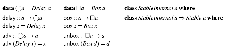
Fig. 10. Implementation of $\mathsf{Rattus}$
primitives.
$\mathsf{Rattus}$
primitives.
If we were to use these primitives as provided by the library, we would end up with the problems illustrated in Section 2. Such an implementation of $\mathsf{Rattus}$
would enjoy none of the operational properties we have proved. To make sure that programs use these primitives according to the typing rules of
$\mathsf{Rattus}$
would enjoy none of the operational properties we have proved. To make sure that programs use these primitives according to the typing rules of $\mathsf{Rattus}$
, our implementation has a second component: a plugin for the GHC Haskell compiler that enforces the typing rules of
$\mathsf{Rattus}$
, our implementation has a second component: a plugin for the GHC Haskell compiler that enforces the typing rules of $\mathsf{Rattus}$
.
$\mathsf{Rattus}$
.
The design of this plugin follows the simple observation that any $\mathsf{Rattus}$
program is also a Haskell program but with more restrictive rules for variable scope and for where
$\mathsf{Rattus}$
program is also a Haskell program but with more restrictive rules for variable scope and for where $\mathsf{Rattus}$
’s primitives may be used. So type-checking a
$\mathsf{Rattus}$
’s primitives may be used. So type-checking a $\mathsf{Rattus}$
program boils down to first type-checking it as a Haskell program and then checking that it follows the stricter variable scope rules. That means, we must keep track of when variables fall out of scope due to the use of
$\mathsf{Rattus}$
program boils down to first type-checking it as a Haskell program and then checking that it follows the stricter variable scope rules. That means, we must keep track of when variables fall out of scope due to the use of $\mathsf{delay}$
,
$\mathsf{delay}$
, ![]() and
and $\mathsf{box}$
, but also due to guarded recursion. Additionally, we must make sure that both guarded recursive calls and
$\mathsf{box}$
, but also due to guarded recursion. Additionally, we must make sure that both guarded recursive calls and ![]() only appear in a context where
only appear in a context where $\checkmark$
is present.
$\checkmark$
is present.
To enforce these additional simple scope rules, we make use of GHC’s plugin API which allows us to customise part of GHC’s compilation pipeline. The different phases of GHC are illustrated in Figure 11 with the additional passes performed by the $\mathsf{Rattus}$
plugin highlighted in bold.
$\mathsf{Rattus}$
plugin highlighted in bold.
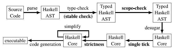
Fig. 11. Compiler phases of GHC (simplified) extended with $\mathsf{Rattus}$
plugin (highlighted in bold).
$\mathsf{Rattus}$
plugin (highlighted in bold).
After type-checking the Haskell abstract syntax tree (AST), GHC passes the resulting typed AST on to the scope-checking component of the $\mathsf{Rattus}$
plugin, which checks the above-mentioned stricter scoping rules. GHC then desugars the typed AST into the intermediate language Core. GHC then performs a number of transformation passes on this intermediate representation, and the first two of these are provided by the
$\mathsf{Rattus}$
plugin, which checks the above-mentioned stricter scoping rules. GHC then desugars the typed AST into the intermediate language Core. GHC then performs a number of transformation passes on this intermediate representation, and the first two of these are provided by the $\mathsf{Rattus}$
plugin: first, we exhaustively apply the two rewrite rules from Section 4.2.1 to transform the program into a single-tick form according to the typing rules of
$\mathsf{Rattus}$
plugin: first, we exhaustively apply the two rewrite rules from Section 4.2.1 to transform the program into a single-tick form according to the typing rules of $\lambda_{\checkmark}$
. Then we transform the resulting code so that
$\lambda_{\checkmark}$
. Then we transform the resulting code so that $\mathsf{Rattus}$
programs adhere to the call-by-value semantics. To this end, the plugin’s strictness pass transforms all lambda abstractions so that they evaluate their arguments to weak head normal form, and all let bindings so that they evaluate the bound expression into weak head normal form. This is achieved by transforming lambda abstractions and let bindings as follows:
$\mathsf{Rattus}$
programs adhere to the call-by-value semantics. To this end, the plugin’s strictness pass transforms all lambda abstractions so that they evaluate their arguments to weak head normal form, and all let bindings so that they evaluate the bound expression into weak head normal form. This is achieved by transforming lambda abstractions and let bindings as follows:
In Haskell Core, case expressions always evaluate the scrutinee to weak head normal form even if there is only a default clause. Hence, this transformation will force the evaluation of x in the lambda abstraction $\lambda x . t$
, and the evaluation of s in the let binding
$\lambda x . t$
, and the evaluation of s in the let binding
![]() . In addition, this strictness pass also checks that
. In addition, this strictness pass also checks that $\mathsf{Rattus}$
code only uses strict data types and issues a warning if lazy data types are used, for example, Haskell’s standard list and pair types. Taken together, the transformations and checks performed by the strictness pass ensure that lambda abstractions, let bindings and data constructors follow the operational semantics of
$\mathsf{Rattus}$
code only uses strict data types and issues a warning if lazy data types are used, for example, Haskell’s standard list and pair types. Taken together, the transformations and checks performed by the strictness pass ensure that lambda abstractions, let bindings and data constructors follow the operational semantics of $\lambda_{\checkmark}$
. The remaining components of the language are either implemented directly as Haskell functions (
$\lambda_{\checkmark}$
. The remaining components of the language are either implemented directly as Haskell functions ( $\mathsf{delay}$
,
$\mathsf{delay}$
, ![]() ,
, $\mathsf{box}$
and
$\mathsf{box}$
and $\mathsf{unbox}$
) and thus require no transformation or use Haskell’s recursion syntax that matches the semantics of the corresponding fixed point combinator in
$\mathsf{unbox}$
) and thus require no transformation or use Haskell’s recursion syntax that matches the semantics of the corresponding fixed point combinator in $\lambda_{\checkmark}$
.
$\lambda_{\checkmark}$
.
However, the Haskell implementation of $\mathsf{delay}$
and
$\mathsf{delay}$
and ![]() do not match the operational semantics of
do not match the operational semantics of $\lambda_{\checkmark}$
exactly. Instead of explicit allocation of delayed computations on a heap that then enables the eager garbage collection strategy of the
$\lambda_{\checkmark}$
exactly. Instead of explicit allocation of delayed computations on a heap that then enables the eager garbage collection strategy of the $\lambda_{\checkmark}$
operational semantics, we rely on Haskell’s lazy evaluation for
$\lambda_{\checkmark}$
operational semantics, we rely on Haskell’s lazy evaluation for $\mathsf{delay}$
and GHC’s standard garbage collection implementation. Since our metatheoretical results show that old temporal data is no longer referenced after each time step, such data will indeed be garbage collected by the GHC runtime system.
$\mathsf{delay}$
and GHC’s standard garbage collection implementation. Since our metatheoretical results show that old temporal data is no longer referenced after each time step, such data will indeed be garbage collected by the GHC runtime system.
Not pictured in Figure 11 is a second scope-checking pass that is performed after the strictness pass. After the single tick pass and thus also after the strictness pass, we expect that the code is typable according to the more restrictive typing rules of $\lambda_{\checkmark}$
. This second scope-checking pass checks this invariant for the purpose of catching implementation bugs in the
$\lambda_{\checkmark}$
. This second scope-checking pass checks this invariant for the purpose of catching implementation bugs in the $\mathsf{Rattus}$
plugin. The Core intermediate language is much simpler than the full Haskell language, so this second scope-checking pass is much easier to implement and much less likely to contain bugs. In principle, we could have saved ourselves the trouble of implementing the much more complicated scope-checking at the level of the typed Haskell AST. However, by checking at this earlier stage of the compilation pipeline, we can provide much more helpful type error messages.
$\mathsf{Rattus}$
plugin. The Core intermediate language is much simpler than the full Haskell language, so this second scope-checking pass is much easier to implement and much less likely to contain bugs. In principle, we could have saved ourselves the trouble of implementing the much more complicated scope-checking at the level of the typed Haskell AST. However, by checking at this earlier stage of the compilation pipeline, we can provide much more helpful type error messages.
One important component of checking variable scope is checking whether types are stable. This is a simple syntactic check: a type
![]() is stable if all occurrences of
is stable if all occurrences of $\bigcirc$
or function types in
$\bigcirc$
or function types in
![]() are nested under a
are nested under a $\square$
. However,
$\square$
. However, $\mathsf{Rattus}$
also supports polymorphic types with type constraints such as in the
$\mathsf{Rattus}$
also supports polymorphic types with type constraints such as in the $\textit{const}$
function:
$\textit{const}$
function:
The $\textit{Stable}$
type class is defined as a primitive in the
$\textit{Stable}$
type class is defined as a primitive in the $\mathsf{Rattus}$
library (see Figure 10). The library does not export the underlying
$\mathsf{Rattus}$
library (see Figure 10). The library does not export the underlying
![]() type class so that the user cannot declare any instances for
type class so that the user cannot declare any instances for $\textit{Stable}$
. Our library does not declare instances of the
$\textit{Stable}$
. Our library does not declare instances of the $\textit{Stable}$
class either. Instead, such instances are derived by the
$\textit{Stable}$
class either. Instead, such instances are derived by the $\mathsf{Rattus}$
plugin that uses GHC’s type checker plugin API, which allows us to provide limited customisation to GHC’s type-checking phase (see Figure 11). Using this API, one can give GHC a custom procedure for resolving type constraints. Whenever GHC’s type checker finds a constraint of the form
$\mathsf{Rattus}$
plugin that uses GHC’s type checker plugin API, which allows us to provide limited customisation to GHC’s type-checking phase (see Figure 11). Using this API, one can give GHC a custom procedure for resolving type constraints. Whenever GHC’s type checker finds a constraint of the form
![]() , it will send it to the
, it will send it to the $\mathsf{Rattus}$
plugin, which will resolve it by performing the above-mentioned syntactic check on
$\mathsf{Rattus}$
plugin, which will resolve it by performing the above-mentioned syntactic check on
![]() .
.
6.2 Using Rattus
To write $\mathsf{Rattus}$
code inside Haskell, one must use GHC with the flag -fplugin=
$\mathsf{Rattus}$
code inside Haskell, one must use GHC with the flag -fplugin= $\mathsf{Rattus}$
.Plugin, which enables the
$\mathsf{Rattus}$
.Plugin, which enables the $\mathsf{Rattus}$
plugin described above. Figure 12 shows a complete program that illustrates the interaction between Haskell and
$\mathsf{Rattus}$
plugin described above. Figure 12 shows a complete program that illustrates the interaction between Haskell and $\mathsf{Rattus}$
. The language is imported via the
$\mathsf{Rattus}$
. The language is imported via the
![]() module, with the
module, with the
![]() module providing a stream library (of which we have seen an excerpt in Figure 1). The program contains only one
module providing a stream library (of which we have seen an excerpt in Figure 1). The program contains only one $\mathsf{Rattus}$
function,
$\mathsf{Rattus}$
function,
![]() , which is indicated by an annotation. This function uses the
, which is indicated by an annotation. This function uses the $\textit{scan}$
combinator to define a stream transducer that sums up its input stream. Finally, we use the
$\textit{scan}$
combinator to define a stream transducer that sums up its input stream. Finally, we use the
![]() function that is provided by the
function that is provided by the
![]() module. It turns a stream function of type
module. It turns a stream function of type
![]() into a Haskell value of type
into a Haskell value of type
![]() defined as follows:
defined as follows:
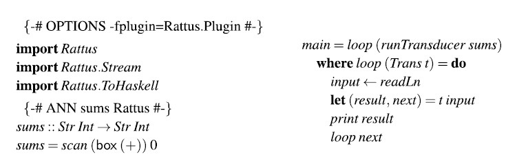
Fig. 12. Complete $\mathsf{Rattus}$
program.
$\mathsf{Rattus}$
program.
This allows us to run the stream function step by step as illustrated in the main function: It reads an integer from the console passes it on to the stream function, prints out the response and then repeats the process.
Alternatively, if a module contains only $\mathsf{Rattus}$
definitions, we can use the annotation
$\mathsf{Rattus}$
definitions, we can use the annotation
to declare that all definitions in a module are to be interpreted as $\mathsf{Rattus}$
code.
$\mathsf{Rattus}$
code.
7 Related work
Embedded FRP languages
The central ideas of FRP were originally developed for the language Fran (Elliott and Hudak Reference Elliott and Hudak1997) for reactive animation. These ideas have since been developed into general-purpose libraries for reactive programming, most prominently the Yampa library (Nilsson et al. Reference Nilsson, Courtney and Peterson2002) for Haskell, which has been used in a variety of applications including games, robotics, vision, GUIs and sound synthesis.
More recently Ploeg and Claessen (2015) have developed the FRPNow! library for Haskell, which – like Fran – uses behaviours and events as FRP primitives (as opposed to signal functions) but carefully restricts the API to guarantee causality and the absence of implicit space leaks. To argue for the latter, the authors construct a denotational model and show using a logical relation that their combinators are not ‘inherently leaky’. The latter does not imply the absence of space leaks, but rather that in principle it can be implemented without space leaks.
While these FRP libraries do not allow direct manipulation of signals since they lack a bespoke type system to make that safe, they do have a practical advantage: their reliance on the host language’s type system makes their implementation and maintenance markedly easier. Moreover, by embedding FRP libraries in host languages with a richer type system, such as full dependent types, one can still obtain some operational guarantees, including productivity (Sculthorpe and Nilsson Reference Sculthorpe and Nilsson2009).
Modal FRP calculi
The idea of using modal type operators for reactive programming goes back to Jeffrey (Reference Jeffrey2012), Krishnaswami and Benton (Reference Krishnaswami and Benton2011), and Jeltsch (Reference Jeltsch2013). One of the inspirations for Jeffrey (Reference Jeffrey2012) was to use linear temporal logic (Pnueli Reference Pnueli1977) as a programming language through the Curry–Howard isomorphism. The work of Jeffrey and Jeltsch has mostly been based on denotational semantics, and to our knowledge Krishnaswami and Benton (Reference Krishnaswami and Benton2011), Krishnaswami et al. (Reference Krishnaswami, Benton and Hoffmann2012), Krishnaswami (Reference Krishnaswami2013), Cave et al. (Reference Cave, Ferreira, Panangaden and Pientka2014), and Bahr et al. (Reference Bahr, Graulund and Møgelberg2019, Reference Bahr, Graulund and Møgelberg2021) are the only works giving operational guarantees. In addition, the calculi of Cave et al. (Reference Cave, Ferreira, Panangaden and Pientka2014) and Bahr et al. (Reference Bahr, Graulund and Møgelberg2021) can encode liveness properties in types by distinguishing between data (least fixed points, e.g., events that must happen within a finite number of steps) and codata (greatest fixed points, e.g., streams). With the help of both greatest and least fixed points, one can express liveness properties of programs in their types (e.g., a server that will always respond within a finite number of time steps). Temporal logic has also been used directly as a specification language for property-based testing and runtime verification of FRP programs (Perez and Nilsson, Reference Perez and Nilsson2020).
Guarded recursive types and the guarded fixed point combinator originate with Nakano (Reference Nakano2000) but have since been used for constructing logics for reasoning about advanced programming languages (Birkedal et al., Reference Birkedal, Møgelberg, Schwinghammer and Støvring2011) using an abstract form of step-indexing (Appel and McAllester, Reference Appel and McAllester2001). The Fitch-style approach to modal types (Fitch, Reference Fitch1952; Clouston, Reference Clouston2018) has been used for guarded recursion in Clocked Type Theory (Bahr et al. Reference Bahr, Grathwohl and Møgelberg2017), where contexts can contain multiple, named ticks. Ticks can be used for reasoning about guarded recursive programs. The denotational semantics of Clocked Type Theory (Mannaa and Møgelberg, Reference Mannaa and Møgelberg2018) reveals the difference from the more standard dual-context approaches to modal logics, such as Dual Intuitionistic Linear Logic (Barber, Reference Barber1996): in the latter, the modal operator is implicitly applied to the type of all variables in one context, in the Fitch-style, placing a tick in a context corresponds to applying a left adjoint to the modal operator to the context. Guatto (Reference Guatto2018) introduced the notion of time warp and the warping modality, generalising the delay modality in guarded recursion, to allow for a more direct style of programming for programs with complex input–output dependencies.
Space leaks
The work by Krishnaswami (Reference Krishnaswami2013) and Bahr et al. (Reference Bahr, Graulund and Møgelberg2019, Reference Bahr, Graulund and Møgelberg2021) is the closest to the present work. Both present a modal FRP language with a garbage collection result similar to ours. Krishnaswami (Reference Krishnaswami2013) pioneered this approach to prove the absence of implicit space leaks but also implemented a compiler for his language, which translates FRP programs into JavaScript. Bahr et al. (Reference Bahr, Graulund and Møgelberg2019) were the first to mechanise the metatheory for a modal FRP calculus, and our mechanisation is based on their work. For a more detailed comparison with these calculi, see Section 4.5.
Krishnaswami et al. (Reference Krishnaswami, Benton and Hoffmann2012) approached the problem of space leaks with an affine type system that keeps track of permission tokens for allocating a stream cons cell. This typing discipline ensures that space usage is bounded by the number of provided permission tokens and thus provides more granular static checks of space usage.
Synchronous dataflow languages, such Esterel (Berry and Cosserat, Reference Berry and Cosserat1985), Lustre (Caspi et al., Reference Caspi, Pilaud, Halbwachs and Plaice1987) and Lucid Synchrone (Pouzet, Reference Pouzet2006), provide even stronger static guarantees – not only on space usage but also on time usage. This feature has made these languages attractive in resource-constrained environments such as hardware synthesis and embedded control software. Their computational model is based on a fixed network of stream processing nodes where each node consumes and produces a statically known number of primitive values at each discrete time step. As a trade-off for these static guarantees, synchronous dataflow languages support neither time-varying values of arbitrary types nor dynamic switching.
8 Discussion and future work
We have shown that modal FRP with strong operational guarantees can be seamlessly integrated into the Haskell programming language. Two main ingredients are central to achieving this integration: (1) the use of Fitch-style typing to simplify the syntax for interacting with the two modalities and (2) lifting some of the restrictions found in previous work on Fitch-style typing systems.
This paper opens up several avenues for future work both on the implementation side and the underlying theory. We chose Haskell as our host language as it has a compiler extension API that makes it easy for us to implement $\mathsf{Rattus}$
and convenient for programmers to start using
$\mathsf{Rattus}$
and convenient for programmers to start using $\mathsf{Rattus}$
with little friction. However, we think that implementing
$\mathsf{Rattus}$
with little friction. However, we think that implementing $\mathsf{Rattus}$
in call-by-value languages like OCaml or F# should be easily achieved by a simple post-processing step that checks the Fitch-style variable scope. This can be done by an external tool (not unlike a linter) that does not need to be integrated into the compiler. Moreover, while the use of the type class
$\mathsf{Rattus}$
in call-by-value languages like OCaml or F# should be easily achieved by a simple post-processing step that checks the Fitch-style variable scope. This can be done by an external tool (not unlike a linter) that does not need to be integrated into the compiler. Moreover, while the use of the type class $\textit{Stable}$
is convenient, it is not necessary as we can always use the
$\textit{Stable}$
is convenient, it is not necessary as we can always use the $\square$
modality instead (cf.
$\square$
modality instead (cf. $\textit{const}$
versus
$\textit{const}$
versus $\textit{constBox}$
). When a program transformation approach is not feasible or not desirable, one can also use
$\textit{constBox}$
). When a program transformation approach is not feasible or not desirable, one can also use $\lambda_{\checkmark}$
rather than
$\lambda_{\checkmark}$
rather than $\lambda_{\checkmark\!\!\checkmark}$
as the underlying calculus. We suspect that most function definitions do not need the flexibility of
$\lambda_{\checkmark\!\!\checkmark}$
as the underlying calculus. We suspect that most function definitions do not need the flexibility of $\lambda_{\checkmark\!\!\checkmark}$
and those that do can be transformed by the programmer with only little syntactic clutter. One could imaging that the type checker could suggest these transformations to the programmer rather than silently performing them itself.
$\lambda_{\checkmark\!\!\checkmark}$
and those that do can be transformed by the programmer with only little syntactic clutter. One could imaging that the type checker could suggest these transformations to the programmer rather than silently performing them itself.
FRP is not the only possible application of Fitch-style type systems. However, most of the interest in Fitch-style system has been in logics and dependent type theory (Clouston, Reference Clouston2018; Birkedal et al., Reference Birkedal, Clouston, Mannaa, Møgelberg, Pitts and Spitters2018; Bahr et al., Reference Bahr, Grathwohl and Møgelberg2017; Borghuis, Reference Borghuis1994) as opposed to programming languages. $\mathsf{Rattus}$
is to our knowledge the first implementation of a Fitch-style programming language. We would expect that programming languages for information control flow (Kavvos, Reference Kavvos2019) and recent work on modalities for pure computations Chaudhury and Krishnaswami (Reference Chaudhury and Krishnaswami2020) admit a Fitch-style presentation and could be implemented similarly to
$\mathsf{Rattus}$
is to our knowledge the first implementation of a Fitch-style programming language. We would expect that programming languages for information control flow (Kavvos, Reference Kavvos2019) and recent work on modalities for pure computations Chaudhury and Krishnaswami (Reference Chaudhury and Krishnaswami2020) admit a Fitch-style presentation and could be implemented similarly to $\mathsf{Rattus}$
.
$\mathsf{Rattus}$
.
While Fitch-style modal FRP languages promise strong static guarantees with only moderate syntactic overhead, we still lack empirical evidence that they help practical adoption of FRP. Our goal with $\mathsf{Rattus}$
is to provide an implementation with a low entry barrier and with access to a mature and practical software development ecosystem. We hope that this enables experimentation with
$\mathsf{Rattus}$
is to provide an implementation with a low entry barrier and with access to a mature and practical software development ecosystem. We hope that this enables experimentation with $\mathsf{Rattus}$
not only by researchers, but also students and practitioners.
$\mathsf{Rattus}$
not only by researchers, but also students and practitioners.
For example, we have looked at only a small fragment of Yampa’s comprehensive arrowised FRP library. A thorough re-implementation of Yampa in $\mathsf{Rattus}$
could provide a systematic comparison of their relative expressiveness. For such an effort, we expect that the signal function type be refined to include the
$\mathsf{Rattus}$
could provide a systematic comparison of their relative expressiveness. For such an effort, we expect that the signal function type be refined to include the $\square$
modality:
$\square$
modality:
This enables the implementation of Yampa’s powerful switch combinators in $\mathsf{Rattus}$
, which among other things can be used to stop a signal function and then resume it (with all its internal state) at a later point. By contrast, it is not clear how such a switch combinator can be provided in an FRP library with first-class streams as presented in Section 3.1.
$\mathsf{Rattus}$
, which among other things can be used to stop a signal function and then resume it (with all its internal state) at a later point. By contrast, it is not clear how such a switch combinator can be provided in an FRP library with first-class streams as presented in Section 3.1.
Part of the success of FRP libraries such as Yampa and FRPNow! is due to the fact that they provide a rich and highly optimised API that integrates well with its host language. In this paper, we have shown that $\mathsf{Rattus}$
can be seamlessly embedded in Haskell, but more work is required to design a comprehensive library and to perform the low-level optimisations that are often necessary to obtain good real-world performance. For example, our definition of signal functions in Section 3.3 resembles the semantics of Yampa’s signal functions, but Yampa’s signal functions are implemented as generalised algebraic data types (GADTs) that can handle some special cases much more efficiently and enable dynamic optimisations.
$\mathsf{Rattus}$
can be seamlessly embedded in Haskell, but more work is required to design a comprehensive library and to perform the low-level optimisations that are often necessary to obtain good real-world performance. For example, our definition of signal functions in Section 3.3 resembles the semantics of Yampa’s signal functions, but Yampa’s signal functions are implemented as generalised algebraic data types (GADTs) that can handle some special cases much more efficiently and enable dynamic optimisations.
In order to devise sound optimisations for $\mathsf{Rattus}$
, we also require suitable coinductive reasoning principles. For example, we might want to make use of Haskell’s rewrite rules to perform optimisations such as map fusion as expressed in the following equation:
$\mathsf{Rattus}$
, we also require suitable coinductive reasoning principles. For example, we might want to make use of Haskell’s rewrite rules to perform optimisations such as map fusion as expressed in the following equation:
Such an equation could be proved sound using step-indexed logical relations, not unlike the one we presented in Section 5. For this to scale, however, we need more high-level reasoning principles such as a sound coinductive axiomatisation of bisimilarity or more generally a suitable type theory with guarded recursion (Møgelberg and Veltri Reference Møgelberg and Veltri2019).
Conflicts of interest
None.
Supplementary material
For supplementary material for this article, please visit https://doi.org/10.1017/S0956796822000132.
A Multi-tick calculus
In this appendix, we give the proof of Theorem 4.1, that is, we show that the program transformation described in Section 4.2.1 indeed transforms any closed $\lambda_{\checkmark\!\!\checkmark}$
term into a closed
$\lambda_{\checkmark\!\!\checkmark}$
term into a closed $\lambda_{\checkmark}$
term.
$\lambda_{\checkmark}$
term.
Figure 13 gives the context formation rules of $\lambda_{\checkmark}$
; the only difference compared to
$\lambda_{\checkmark}$
; the only difference compared to $\lambda_{\checkmark\!\!\checkmark}$
is the rule for adding ticks, which has a side condition so that there may be no more than one tick. Figure 14 lists the full set of typing rules of
$\lambda_{\checkmark\!\!\checkmark}$
is the rule for adding ticks, which has a side condition so that there may be no more than one tick. Figure 14 lists the full set of typing rules of $\lambda_{\checkmark}$
. Compared to
$\lambda_{\checkmark}$
. Compared to $\lambda_{\checkmark\!\!\checkmark}$
(cf. Figure 5), the only rules that have changed are the rule for lambda abstraction, and the rule for
$\lambda_{\checkmark\!\!\checkmark}$
(cf. Figure 5), the only rules that have changed are the rule for lambda abstraction, and the rule for $\mathsf{delay}$
. Both rules transform the context
$\mathsf{delay}$
. Both rules transform the context $\Gamma$
to
$\Gamma$
to $\vert\Gamma\vert$
, which removes the
$\vert\Gamma\vert$
, which removes the $\checkmark$
in
$\checkmark$
in $\Gamma$
if it has one:
$\Gamma$
if it has one:
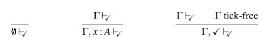
Fig. 13. Well-formed contexts of $\lambda_{\checkmark}$
.
$\lambda_{\checkmark}$
.
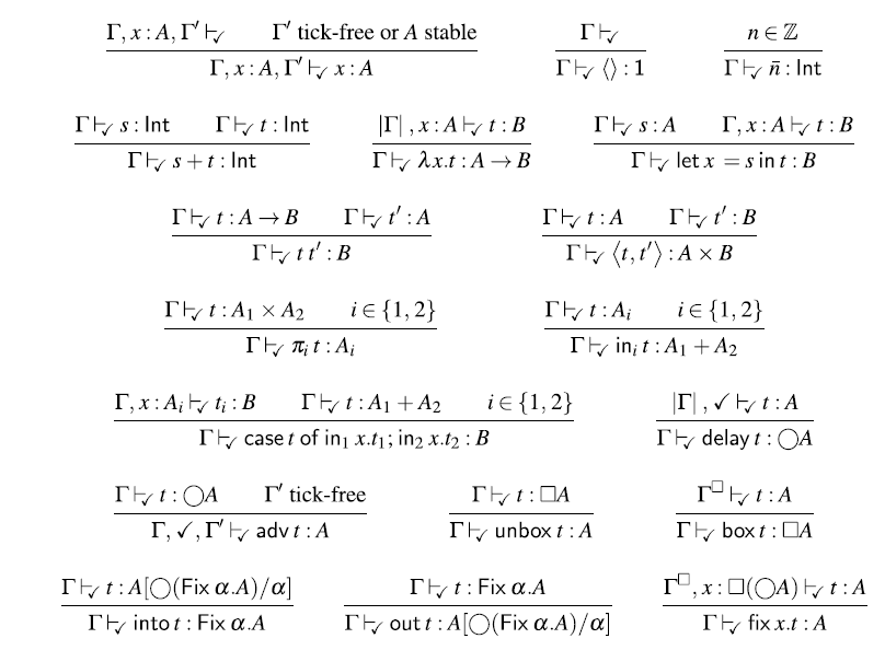
Fig. 14. Typing rules of $\lambda_{\checkmark}$
.
$\lambda_{\checkmark}$
.
We define the rewrite relation $\longrightarrow$
as the least relation that is closed under congruence and the following rules:
$\longrightarrow$
as the least relation that is closed under congruence and the following rules:
where K is a term with a single occurrence of a hole [] that is not in the scope of $\mathsf{delay}$ $\mathsf{adv}$
,
$\mathsf{adv}$
, $\mathsf{box}$
,
$\mathsf{box}$
, $\mathsf{fix}$
, or a lambda abstraction. Formally, K is generated by the following grammar:
$\mathsf{fix}$
, or a lambda abstraction. Formally, K is generated by the following grammar:
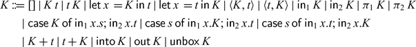
We write K[t] to substitute the unique hole [] in K with the term t.
In the following, we show that for each $\vdash_{\checkmark\!\!\checkmark}{t}:{A}$
, if we exhaustively apply the above rewrite rules to t, we obtain a term
$\vdash_{\checkmark\!\!\checkmark}{t}:{A}$
, if we exhaustively apply the above rewrite rules to t, we obtain a term $\vdash_{\checkmark\!\!\checkmark}{t'}:{A}$
. We prove this by proving each of the following properties in turn:
$\vdash_{\checkmark\!\!\checkmark}{t'}:{A}$
. We prove this by proving each of the following properties in turn:
-
(1) Subject reduction: If
${\Gamma}\vdash_{\checkmark\!\!\checkmark}{s}:{A}$
and
$s \longrightarrow t$
, then
${\Gamma}\vdash_{\checkmark\!\!\checkmark}{t}:{A}$
. -
(2) Exhaustiveness: If t is a normal form for
$\longrightarrow$
, then
$\vdash_{\checkmark}{t}:{A}$
implies
$\vdash_{\checkmark}{t}:{A}$
. -
(3) Strong normalisation: There is no infinite
$\longrightarrow$
-reduction sequence.


A.1 Subject reduction
We first show subject reduction (cf. Proposition A.4 below). To this end, we need a number of lemmas:
Lemma A.1 (weakening) Let
![]() and
and $\Gamma$
tick-free. Then
$\Gamma$
tick-free. Then
![]() .
.
Proof. By straightforward induction on
![]() .
.
Lemma A.2 Given $\Gamma,\checkmark,\Gamma'\vdash_{\checkmark\!\!\checkmark}{K\lbrack\mathrm{adv}\,t\rbrack\,s}:A$
with
$\Gamma,\checkmark,\Gamma'\vdash_{\checkmark\!\!\checkmark}{K\lbrack\mathrm{adv}\,t\rbrack\,s}:A$
with $\Gamma'$
tick-free, then there is some type B such that
$\Gamma'$
tick-free, then there is some type B such that $\Gamma\vdash_{\checkmark\!\!\checkmark}t:\bigcirc B$
and
$\Gamma\vdash_{\checkmark\!\!\checkmark}t:\bigcirc B$
and $\Gamma,x:\bigcirc B,\checkmark,\Gamma'\vdash_{\!\!\checkmark\!\!\checkmark}{K\lbrack\mathrm{adv}\,x\rbrack}A$
.
$\Gamma,x:\bigcirc B,\checkmark,\Gamma'\vdash_{\!\!\checkmark\!\!\checkmark}{K\lbrack\mathrm{adv}\,x\rbrack}A$
.
Proof We proceed by induction on the structure of K.
-
$\underline{[]:}$
$\Gamma,\checkmark,\Gamma'\vdash_{\checkmark\!\!\checkmark}\mathrm{adv}\,t:A$
and
$\Gamma'$
tick-free implies that
$\Gamma\vdash_{\!\checkmark\!\!\checkmark}\,t:\bigcirc A$
. Moreover, given a fresh variable x, we have that
$\Gamma,x:\bigcirc A\vdash_{\!\checkmark\!\!\checkmark}x:\bigcirc A$
, and thus
$\Gamma,x:\bigcirc A,\checkmark,\Gamma'\vdash_{\!\checkmark\!\!\checkmark}\mathrm{adv}\,x:A$
and
$\Gamma'$
.
-
$\underline{K\,s:}$
$\Gamma,\checkmark,\Gamma'\vdash_{\checkmark\!\!\checkmark}{K\lbrack\mathrm{adv}\,t\rbrack\,s}:A$
implies that there is some A’ with
$\Gamma,\checkmark,\Gamma'\vdash_{\checkmark\!\!\checkmark}s:A'$
and
$\Gamma,\checkmark,\Gamma'\vdash_{\!\!\checkmark\!\!\checkmark}{K\lbrack\mathrm{adv}\,t\rbrack}:{A'\rightarrow A}$
. By induction hypothesis, the latter implies that there is some B with
$\Gamma\vdash_{\checkmark\!\!\checkmark}t:\bigcirc B$
and
. Hence,
, by Lemma A.1, and thus
.
-
$\underline{s\,K:}$
implies that there is some A’ with
and
. By induction hypothesis, the latter implies that there is some B with
and
. Hence,
, by Lemma A.1, and thus
.
-
implies that there is some A’ with
. By induction hypothesis, the latter implies that there is some B with
and
. Hence,
, by Lemma A.1, and thus
${\Gamma,x }:$
.
-
implies that there is some A’ with
. By induction hypothesis, the latter implies that there is some B with
. Hence,
, by Lemma A.1, and thus
.


The remaining cases follow by induction hypothesis and Lemma A.1 in a manner similar to the cases above.
Lemma A.3 Let
![]() and
and $\Gamma'$
tick-free. Then there is some type B such that
$\Gamma'$
tick-free. Then there is some type B such that
![]() and
and
![]() .
.
Proof We proceed by induction on the structure of K:
-
and
$\Gamma'$
tick-free implies that there must be
$\Gamma_1$
and
$\Gamma_2$
such that
$\Gamma_2$
is tick-free,
$\Gamma= \Gamma_1,\checkmark,\Gamma_2$
, and
$\Gamma_1\vdash_{\!\!\checkmark\!\!\checkmark}t:\bigcirc A$
. Hence,
$\Gamma_1,\checkmark,\Gamma_2\vdash_{\!\!\checkmark\!\!\checkmark}\mathrm{adv}t:A$
. Moreover,
$\Gamma,x:A,\Gamma'\vdash_{\!\!\checkmark\!\!\checkmark}x:A$
follows immediately by the variable introduction rule.
-
implies that there is some A’ with
and
. By induction hypothesis, the latter implies that there is some B with
and
. Hence,
, by Lemma A.1, and thus
.
-
implies that there is some A’ with
and
. By induction hypothesis, the latter implies that there is some B with
and
$\Gamma,x:B,\Gamma',y:A'\vdash_{\!\!\checkmark\!\!\checkmark}{K\lbrack x\rbrack}:A$
. Hence,
${\Gamma,x: B, \Gamma'}\vdash_{\checkmark\!\!\checkmark}{s}:{A'}$
, by Lemma A.1, and thus
.


The remaining cases follow by induction hypothesis and Lemma A.1 in a manner similar to the cases above.
Proposition A.4 (subject reduction). If $\Gamma\vdash_{\!\!\checkmark\!\!\checkmark}s:A$
and
$\Gamma\vdash_{\!\!\checkmark\!\!\checkmark}s:A$
and $s \longrightarrow t$
, then
$s \longrightarrow t$
, then $\Gamma\vdash_{\!\!\checkmark\!\!\checkmark}t:A$
.
$\Gamma\vdash_{\!\!\checkmark\!\!\checkmark}t:A$
.
Proof. We proceed by induction on $s \longrightarrow t$
.
$s \longrightarrow t$
.
-
Let
$s \longrightarrow t$
be due to congruence closure. Then,
$\Gamma\vdash_{\!\!\checkmark\!\!\checkmark}t:A$
follows by the induction hypothesis. For example, if
$s = s_1\,s_2$
,
$t= t_1\,s_2$
and
$s_1 \longrightarrow t_1$
, then we know that
$\Gamma\vdash_{\!\!\checkmark\!\!\checkmark}s_1:{B\rightarrow A}$
and
$\Gamma\vdash_{\!\!\checkmark\!\!\checkmark}s_2:B$
for some type B. By induction hypothesis, we then have that
$\Gamma\vdash_{\!\!\checkmark\!\!\checkmark}t_1:{B\rightarrow A}$
and thus
$\Gamma\vdash_{\!\!\checkmark\!\!\checkmark}t:A$
. -
Let
and
. That is,
$A = \bigcirc A'$
and
$\Gamma,\checkmark\vdash_{\!\!\checkmark\!\!\checkmark}{K\lbrack\mathrm{adv}\,t\rbrack}:A'$
. Then by Lemma A.2, we obtain some type B such that
$\Gamma\vdash_{\checkmark\!\!\checkmark}t:\bigcirc B$
and
. Hence,
. -
Let
and
. Hence,
$A = A_1 \to A_2$
and
. Then, by Lemma A.3, there is some type B such that
and
. Hence,
.


A.2 Exhaustiveness
Secondly, we show that any closed $\lambda_{\!\!\checkmark\!\!\checkmark}$
term that cannot be rewritten any further is also a closed
$\lambda_{\!\!\checkmark\!\!\checkmark}$
term that cannot be rewritten any further is also a closed $\lambda_{\checkmark}$
term (cf. Proposition A.9 below).
$\lambda_{\checkmark}$
term (cf. Proposition A.9 below).
Definition A.5
-
(i) We say that a term t is weakly adv-free iff whenever
$t = K[\mathsf{adv}\,s]$
for some K and s, then s is a variable. -
(ii) We say that a term t is strictly adv-free iff there are no K and s such that
$t = K[\mathsf{adv}\,s]$
.


Clearly, any strictly $\mathsf{adv}$
-free term is also weakly
$\mathsf{adv}$
-free term is also weakly $\mathsf{adv}$
-free.
$\mathsf{adv}$
-free.
In the following, we use the notation
![]() to denote the fact that there is no term t’ with
to denote the fact that there is no term t’ with
![]() ; in other words, t is a normal form.
; in other words, t is a normal form.
Lemma A.6
-
(i) If
, then t is weakly
$\mathsf{adv}$
-free. -
(ii) If
, then t is strictly
$\mathsf{adv}$
-free.


Proof Immediate, by the definition of weakly/strictly $\mathsf{adv}$
-free and
$\mathsf{adv}$
-free and
![]() .
.
Lemma A.7 Let $\Gamma'$
contain at least one tick,
$\Gamma'$
contain at least one tick,
![]() , and t weakly
, and t weakly $\mathsf{adv}$
-free. Then
$\mathsf{adv}$
-free. Then
![]()
Proof We proceed by induction on ${\Gamma,\checkmark,\Gamma'}\vdash_{\checkmark\!\!\checkmark}{t}:{A}$
:
${\Gamma,\checkmark,\Gamma'}\vdash_{\checkmark\!\!\checkmark}{t}:{A}$
:
-
Then there are
$\Gamma_1,\Gamma_2$
such that
$\Gamma_2$
tick-free,
$\Gamma' = \Gamma_1,\checkmark,\Gamma_2$
, and
. Since
$\mathsf{adv}\,t$
is by assumption weakly
$\mathsf{adv}$
-free, we know that t is some variable x. Since
$\bigcirc A$
is not stable we thus know that
$x:\bigcirc A \in \Gamma_1$
. Hence,
, and therefore
.
-
Hence,
. Moreover, since
, we have by Lemma A.6 that t is weakly
$\mathsf{adv}$
-free. We may thus apply the induction hypothesis to obtain that
. Hence,
.
-
Hence,
, which is the same as
. Hence,
.
-
That is,
. Since, by assumption
, we know by Lemma A.6 that t is strictly
$\mathsf{adv}$
-free, and thus also weakly
$\mathsf{adv}$
-free. Hence, we may apply the induction hypothesis to obtain that
$\Gamma^\square,\Gamma',x:A\vdash_{\!\!\checkmark\!\!\checkmark}t:B$
, which in turn implies
.
-
Hence,
, which is the same as
. Hence,
.
-
Then, either
. In either case,
${\Gamma^{\square},\Gamma'}\vdash_{\checkmark\!\!\checkmark}{x}:{A}$
follows.
-
The remaining cases follow by the induction hypothesis in a straightforward manner. For example, if
, then there is some type B with
$\Gamma,\checkmark,\Gamma'\vdash_{\!\!\checkmark\!\!\checkmark}s:{B\rightarrow A}$
and
. Since
$s\,t$
is weakly
$\mathsf{adv}$
-free, so are s and t, and we may apply the induction hypothesis to obtain that
and
$\Gamma^\square,\Gamma'\vdash_{\!\!\checkmark\!\!\checkmark}t:B$
. Hence,
$\Gamma^\square,\Gamma'\vdash_{\!\!\checkmark\!\!\checkmark}s\,t:A$
.


Lemma A.8 Let
![]() and t strictly
and t strictly $\mathsf{adv}$
-free. Then
$\mathsf{adv}$
-free. Then
![]() .
.
(Note that this Lemma is about $\lambda_{\checkmark}$
.)
$\lambda_{\checkmark}$
.)
Proof We proceed by induction on
![]() .
.
-
Impossible since
$\mathsf{adv}\,t$
is not strictly
$\mathsf{adv}$
-free.
-
Hence,
, which in turn implies that
.
-
Hence,
, which is the same as
. Hence,
.
-
That is,
. Since, by assumption
, we know by Lemma A.6 that t is strictly
$\mathsf{adv}$
-free. Hence, we may apply the induction hypothesis to obtain that
, which in turn implies
.
-
Hence,
, which is the same as
. Hence,
.
-
Then, either
. In either case,
A follows.
-
The remaining cases follow by the induction hypothesis in a straightforward manner. For example, if
, then there is some type B with
$\Gamma,\checkmark,\Gamma'\vdash_{\!\!\checkmark}s:{B\rightarrow A}$
and
. Since
$s\,t$
is strictly
$\mathsf{adv}$
-free, so are s and t, and we may apply the induction hypothesis to obtain that
and
$\Gamma^\square,\Gamma'\vdash_{\!\!\checkmark}t:B$
. Hence,
$\Gamma^\square,\Gamma'\vdash_{\!\!\checkmark}s\,t:A$
.


In order for the induction argument to go through, we generalise the exhaustiveness property from closed $\lambda_{\checkmark\!\!\checkmark}$
terms to open
$\lambda_{\checkmark\!\!\checkmark}$
terms to open $\lambda_{\checkmark\!\!\checkmark}$
terms in a context with at most one tick.
$\lambda_{\checkmark\!\!\checkmark}$
terms in a context with at most one tick.
Proposition A.9 (exhaustiveness) Let $\Gamma\vdash_{\!\!\checkmark}$
,
$\Gamma\vdash_{\!\!\checkmark}$
, $\Gamma\vdash_{\!\!\checkmark\!\!\checkmark}t:A$
and
$\Gamma\vdash_{\!\!\checkmark\!\!\checkmark}t:A$
and
![]() . Then
. Then ${\Gamma}\vdash_{\!\!\checkmark}{t}:{A}$
.
${\Gamma}\vdash_{\!\!\checkmark}{t}:{A}$
.
Proof We proceed by induction on the structure of t and by case distinction on the last typing rule in the derivation of $\Gamma\vdash_{\!\!\checkmark\!\!\checkmark}t:A$
.
$\Gamma\vdash_{\!\!\checkmark\!\!\checkmark}t:A$
.
-
We consider two cases:
-
$\Gamma$
is tick-free: Hence,
and thus
by induction hypothesis. Since
, we thus have that
.
-
$\Gamma=\Gamma_1,\checkmark,\Gamma_2$
and
$\Gamma_2$
tick-free: By definition,
and, by Lemma A.6, t is weakly
$\mathsf{adv}$
-free. Hence, by Lemma A.7, we have that
. We can thus apply the induction hypothesis to obtain that
. Since
, we thus have that
.
-
-
By induction hypothesis, we have that
. There are two cases to consider:
-
$\Gamma$
is tick-free: Then,
and we thus obtain that
.
-
with
$\Gamma_1,\Gamma_2$
tick-free: Since
by definition and t strictly
$\mathsf{adv}$
-free by Lemma A.6, we may apply Lemma A.8 to obtain that
. Since
, we thus have that
.
-
-
All remaining cases follow immediately from the induction hypothesis, because all other rules are either the same for both calculi or the
$\lambda_{\checkmark}$
typing rule has an additional side condition that
$\Gamma$
have at most one tick, which holds by assumption.


A.3 Strong normalisation
Proposition A.10 (strong normalisation) The rewrite relation $\longrightarrow$
is strongly normalising.
$\longrightarrow$
is strongly normalising.
Proof To show that $\longrightarrow$
is strongly normalising, we define for each term t a natural number d(t) such that, whenever
$\longrightarrow$
is strongly normalising, we define for each term t a natural number d(t) such that, whenever $t \longrightarrow t'$
, then
$t \longrightarrow t'$
, then $d(t) > d(t')$
. A redex is a term of the form
$d(t) > d(t')$
. A redex is a term of the form $\mathsf{delay}\,K[\mathsf{adv}\,t]$
with t not a variable, or a term of the form
$\mathsf{delay}\,K[\mathsf{adv}\,t]$
with t not a variable, or a term of the form $\lambda\, x.K[\mathsf{adv}\,s]$
. For each redex occurrence in a term t, we can calculate its depth as the length of the unique path that goes from the root of the abstract syntax tree of t to the occurrence of the redex. Define d(t) as the sum of the depth of all redex occurrences in t. Since each rewrite step
$\lambda\, x.K[\mathsf{adv}\,s]$
. For each redex occurrence in a term t, we can calculate its depth as the length of the unique path that goes from the root of the abstract syntax tree of t to the occurrence of the redex. Define d(t) as the sum of the depth of all redex occurrences in t. Since each rewrite step $t \longrightarrow t'$
removes a redex or replaces a redex with a new redex at a strictly smaller depth, we have that
$t \longrightarrow t'$
removes a redex or replaces a redex with a new redex at a strictly smaller depth, we have that $d(t) > d(t')$
.
$d(t) > d(t')$
.
Theorem A.11. For each $\vdash_{\!\!\checkmark\!\!\checkmark}{t}:{A}$
, we can effectively construct a term t’ with
$\vdash_{\!\!\checkmark\!\!\checkmark}{t}:{A}$
, we can effectively construct a term t’ with $t \longrightarrow^* t'$
and
$t \longrightarrow^* t'$
and $\vdash_{\!\!\checkmark}{t'}:{A}$
.
$\vdash_{\!\!\checkmark}{t'}:{A}$
.
Proof We construct t’ from t by repeatedly applying the rewrite rules of $\longrightarrow$
. By Proposition A.10, this procedure will terminate and we obtain a term t’ with
$\longrightarrow$
. By Proposition A.10, this procedure will terminate and we obtain a term t’ with $t \longrightarrow^* t'$
and
$t \longrightarrow^* t'$
and
![]() . According to Proposition A.4, this means that
. According to Proposition A.4, this means that $\vdash_{\!\!\checkmark\!\!\checkmark}{t'}:{A}$
, which in turn implies by Proposition A.9 that
$\vdash_{\!\!\checkmark\!\!\checkmark}{t'}:{A}$
, which in turn implies by Proposition A.9 that $\vdash_{\!\!\checkmark}{t'}:{A}$
.
$\vdash_{\!\!\checkmark}{t'}:{A}$
.
B Coq formalisation
The supplementary material for this article contains a Coq formalisation of our meta-theoretical results. Below we give a high-level overview of the structure of the formalisation.
Main results
The main results are proved in the following three Coq files:
-
FundamentalProperty.v proves Theorem 5.1, the fundamental property of the logical relation.
-
Productivity.v proves Theorem 4.2, that is, the stream semantics is safe.
-
Causality.v proves Theorem 4.3, that is, the stream transducer semantics is safe.
Language definition
The following files define the $\lambda_{\checkmark}$
calculus and prove auxiliary lemmas:
$\lambda_{\checkmark}$
calculus and prove auxiliary lemmas:
-
RawSyntax.v defines the syntax of
$\lambda_{\checkmark}$
. -
Substitutions.v defines substitutions of types and terms.
-
Typing.v defines the type system of
$\lambda_{\checkmark}$
. -
Reduction.v defines the big-step operational semantics.
-
Streams.v defines the small-step operational semantics for streams and stream transducers.


Logical relation
The following files contain the central definitions and lemmas for the logical relation argument:
-
Heaps.v defines heaps.
-
Worlds.v defines stores and the various orderings that are used in the logical relation.
-
LogicalRelation.v defines the logical relation and proves characterisation lemmas that correspond to the definition of the logical relation in Figure 9.
-
LogicalRelationAux.v proves lemmas about the logical relation that are used in the proof of the fundamental property.
Further details about the formalisation can be found in the accompanying README file.


 Open access
Discussions
No Discussions have been published for this article.