


1 Introduction
Besides calculus, linear algebra has always been present as a valuable mathematical tool for engineering and physics. Seemingly unrelated technologies are inherently linear algebraic: e.g., the Google PageRank concept is an eigenvector, and numerical linear algebra algorithms are at the core of convex optimization. Further afield, linear algebra is the backbone of much of modern mathematical physics; e.g., non-linear differential equations are solved by iterating linear systems. It is difficult to overstate the sheer practicality of linear algebra theory and its influence in shaping modern science.
On the other hand, in computer science, the main mathematical tools have been more discrete rather than quantitative with logic, functions, relations, graphs, and combinatorics. Lately there is evidence of a shift towards integrating linear algebra into computing, with examples in machine learning, process semantics, quantum programming, natural language semantics, and data mining. This trend suggests a growing interest in applying linear algebra techniques to computing, driven by diverse research areas. For instance, many techniques in natural language processing, such as word2vec, aim to represent data as vectors in a suitable vector space; semantic relationship between words is thus captured by the usual euclidean distance formula. Other techniques can be cited, such as co-occurrence matrices which quantify how often words appear together in a body of text and works by Baroni & Zamparelli (Reference Baroni and Zamparelli2010) on adjective-noun composition, where nouns are represented by vectors and adjectives by matrices. Matrix multiplication lies at the heart of neural networks. The trendy attention mechanism of the Transformer Architecture (Vaswani et al., Reference Vaswani, Shazeer, Parmar, Uszkoreit, Jones, Gomez, Kaiser and Polosukhin2023), which enabled much of modern generative models such as ChatGPT and Stable Diffusion, is computed using dot products. Quantum computing and non-deterministic programming in general are also making use of linear algebra techniques, as for example in the paper by Sernadas et al. (Reference Sernadas, Ramos and Mateus2008) a method for deciding correctness of probabilistic programs is devised.
It is well known among the purist computer scientists that categorical (abstracting the data type), index-free, calculational reasoning and program derivation are good practices. Thus, it is natural to inquire whether linear algebra, with its recently popularized status as a programming tool, can also benefit from such practices. This can be found in the literature, see e.g. Gonthier (Reference Gonthier2011), Mac Lane (Reference Mac Lane2013). As our main example, Macedo & Oliveira (Reference Macedo and Oliveira2013) achieve point-free calculational reasoning in linear algebra by presenting the fundamental laws of matrix algebra as rewriting rules.
Relations and relational reasoning have already proven to be very important in programming (Bird & De Moor, Reference Bird and De Moor1996). As a natural extension of the ideas of Macedo and Oliveira, the aim of this paper is to showcase an approach for linear algebra where, instead of matrices, the main object of study is that of a linear relation (Arens, Reference Arens1961; Mac Lane, Reference Mac Lane1961; Coddington, Reference Coddington1973; Cross, Reference Cross1998). It generalizes the notion of a linear transformation in the same sense that ordinary relations generalize the notion of a function. We thereby quote from algebra of programming: “Our framework is relational because we need a degree of freedom in specification and proof that a calculus of functions alone would not provide.” As we shall see in later sections, there is much to gain by also introducing the relational paradigm into linear algebra.
Our proofs make use of string diagrams. They are popular objects among category theorists, and are essentially formally defined drawings with certain rules for combining them (Selinger, Reference Selinger2011; Baez & Erbele, Reference Baez and Erbele2015). It is well known that string diagrams are a good tool for point-free reasoning and type-checking. Also, their graphical 2d-syntax allows one to omit parentheses around the two ways of composing relations, much like the usual 1d-syntax dismisses parentheses when functions are composed. Their use in linear algebra has recently been explored by Zanasi (Reference Zanasi2015), who developed what is called graphical linear algebra (GLA).
In Section 2, differences among the three notations used in this paper are discussed (which will be called pointwise, classical, and graphical). Tables 3 and 4, referred to as the Dictionary of Notations, show how to translate one into another. Additionally, this section exposes the main axioms and theorems that will be employed throughout this text, presenting their respective representations in the three notations.
In Sections 3 and 4, our approach is to proceed primarily by example. In Section 3, we construct proofs through verification. Two algorithms are explored: an algorithm for finding fundamental bases for the subspaces of a matrix (Beezer, Reference Beezer2014) and the Zassenhaus algorithm (Fischer, Reference Fischer2012). Section 4 shows two examples of program derivation and one last example where a property is derived instead. Two additional examples will be presented: calculating the right inverse of a wide triangular matrix and switching from implicit to explicit basis (solving a homogeneous linear system). The pseudocode for each algorithm (which will be a systematic translation of the proof steps) will be provided. Lastly, a proof of a result concerning the duality between Gaussian elimination and the exchange lemma will also be presented (Barańczuk & Szydło, 2021).
1.1 The category of linear relations
Point-free, calculational approaches for program derivation in linear algebra have already been explored in a previous work by Macedo & Oliveira (Reference Macedo and Oliveira2013). The authors present the fundamental laws of matrix algebra and show how blocked matrix notation permits point-free equational reasoning and algorithm derivation in matrix algebra. Their approach makes use of the rich biproduct structure of $\textsf{FinVect}_\textsf{k}$
(where
$\textsf{FinVect}_\textsf{k}$
(where $\textsf{k}$
stands for a field), a category whose arrows are linear transformations. Below is the full definition. In this paper, for simplicity, we will always consider
$\textsf{k}$
stands for a field), a category whose arrows are linear transformations. Below is the full definition. In this paper, for simplicity, we will always consider $\textsf{k} = \mathbb{R}$
.
$\textsf{k} = \mathbb{R}$
.
Definition 1 ( $\textsf{FinVect}_{\mathbb{R}}$
) The category
$\textsf{FinVect}_{\mathbb{R}}$
is such that
$\textsf{FinVect}_{\mathbb{R}}$
) The category
$\textsf{FinVect}_{\mathbb{R}}$
is such that
-
• the objects are finite-dimensional vector spaces over $\mathbb{R}$
,
$\mathbb{R}$
, -
• the arrows are linear transformations between them,
-
• composition stands for composition of functions,
-
• the identity arrow is the identity map.

Despite its efficacy, subspaces appear only at the object level in $\textsf{FinVect}_{\mathbb{R}}$
, whereas arrows exclusively represent linear transformations. This setup poses challenges for point-free reasoning (without referencing objects) about subspaces. It is well known that when one wants point-free reasoning about relations, such as in relational algebra, it is a good idea to use the category of relations (
$\textsf{FinVect}_{\mathbb{R}}$
, whereas arrows exclusively represent linear transformations. This setup poses challenges for point-free reasoning (without referencing objects) about subspaces. It is well known that when one wants point-free reasoning about relations, such as in relational algebra, it is a good idea to use the category of relations ( $\textsf{Rel}$
), instead of the category of functions (
$\textsf{Rel}$
), instead of the category of functions ( $\textsf{Set}$
) (Bird & De Moor, Reference Bird and De Moor1996). In a similar vein, one may naturally inquire about the analogy of
$\textsf{Set}$
) (Bird & De Moor, Reference Bird and De Moor1996). In a similar vein, one may naturally inquire about the analogy of $\textsf{Rel}$
in regards to
$\textsf{Rel}$
in regards to $\textsf{FinVect}_{\mathbb{R}}$
. One possible solution is the category
$\textsf{FinVect}_{\mathbb{R}}$
. One possible solution is the category $\textsf{LinRel}_{\mathbb{R}}$
(Zanasi, Reference Zanasi2015; Baez & Erbele, Reference Baez and Erbele2015), in which the arrows represent linear relations (a generalization of both linear transformations and subspaces).
$\textsf{LinRel}_{\mathbb{R}}$
(Zanasi, Reference Zanasi2015; Baez & Erbele, Reference Baez and Erbele2015), in which the arrows represent linear relations (a generalization of both linear transformations and subspaces).
Definition 2 ( $\textsf{LinRel}_{\mathbb{R}}$
). Given vector spaces X and Y over
$\textsf{LinRel}_{\mathbb{R}}$
). Given vector spaces X and Y over $\mathbb{R}$
, a linear relation R between them is a subspace of the product space
$\mathbb{R}$
, a linear relation R between them is a subspace of the product space $X \times Y$
. There are two main ways of composing these objects, called relational composition and cartesian product.
$X \times Y$
. There are two main ways of composing these objects, called relational composition and cartesian product.
-
• Relational composition: Let
$R \subseteq X \times Z$
and
$S \subseteq Z \times Y$
be two linear relations. Define their composition
$SR \subseteq X \times Y$
as .
\[SR := \{(x, y) \;|\; \exists z \text{ such that } (x, z) \in R, (z, y) \in S\}.\]
-
• Cartesian product: Let
$R \subseteq A \times B$
and
$S \subseteq X \times Y$
be two linear relations. Define their cartesian product
$R \times S \subseteq (A \times X) \times (B \times Y)$
as
\[R \times S := \{((a, x), (b, y)) \;|\; (a, b) \in R, (x, y) \in S\}.\]


The category LinRel $_{\mathbb{R}}$
is such that
$_{\mathbb{R}}$
is such that
-
• the objects are finite-dimensional vector spaces over
$\mathbb{R}$
, -
• the arrows are linear relations between them,
-
• composition stands for relational composition,
-
• the identity arrow of an object X is the identity relation
$\{(x, x) \;|\; x \in X\} \subseteq X \times X$
.


Definition 3 (Opposite). Given a relation $R \subseteq X \times Y$
, we define its opposite
$R \subseteq X \times Y$
, we define its opposite $R^o \subseteq Y \times X$
as
$R^o \subseteq Y \times X$
as
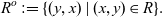 \[R^o := \{(y, x) \;|\; (x, y) \in R\}.\]
Linear transformations and vector spaces can be thought of as special cases of linear relations. The representation of a linear transformation $T: X \rightarrow Y$
as a linear relation is its graph
$T: X \rightarrow Y$
as a linear relation is its graph $\{(x, Tx) \;|\; x \in X \}$
. A subspace
$\{(x, Tx) \;|\; x \in X \}$
. A subspace $X \subseteq Y$
can be thought of as the relation
$X \subseteq Y$
can be thought of as the relation $\{*\} \times X \subseteq \{*\} \times Y$
where
$\{*\} \times X \subseteq \{*\} \times Y$
where $\{*\}$
is the zero-dimensional space. When restricted to linear transformations, relational composition, and cartesian product yield the usual composition and cartesian product of linear transformations. Composing a linear subspace with a linear transformation corresponds to applying the transformation to the subspace. For simplicity, we will make no distinction between these objects and their representation as linear relations.
$\{*\}$
is the zero-dimensional space. When restricted to linear transformations, relational composition, and cartesian product yield the usual composition and cartesian product of linear transformations. Composing a linear subspace with a linear transformation corresponds to applying the transformation to the subspace. For simplicity, we will make no distinction between these objects and their representation as linear relations.
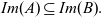
Example 1. (Image). Given a linear transformation $A: X \rightarrow Y$
, we can represent the image of A as the composition
$A: X \rightarrow Y$
, we can represent the image of A as the composition
 \begin{align*} AX &\;= \{(*, x) \;|\; \exists z \text{ such that } (*, z) \in X, (z, x) \in A\} \\ &\;= \{(*, x) \;|\; \exists z \in X \text{ such that } Az = x\} \\ &\;= \{(*, x) \;|\; x \in Im(A)\} \\ &\;= Im(A). \end{align*}
We may extend the notion of blocked matrices to linear relations.
Definition 4 (Blocked relations).
 \[\begin{bmatrix} R & S \end{bmatrix} := \{((x, y), z+w) \;|\; (x, z) \in R, (y, w) \in S\}\]
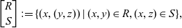 \[\begin{bmatrix} R \\ S \end{bmatrix} := \{(x, (y, z)) \;|\; (x, y) \in R, (x, z) \in S\},\]
 \[R + S := \{(x, y+z) \;|\; (x, y) \in R, (x, z) \in S\}.\]
Note that when U and V are subspaces, the operation $(U, V) \mapsto U + V$
corresponds to the usual sum of linear subspaces, i.e.
$(U, V) \mapsto U + V$
corresponds to the usual sum of linear subspaces, i.e. $U + V = \{ v+w \mid v \in U, w \in V \}$
. In this case, we also have the identities
$U + V = \{ v+w \mid v \in U, w \in V \}$
. In this case, we also have the identities
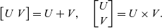 \[\begin{bmatrix} U & V \end{bmatrix} = U + V, \quad \begin{bmatrix} U \\ V \end{bmatrix} = U \times V.\]
1.2 Relational algebra unifies matrix and subspace laws
All matrix algebra rules from Macedo & Oliveira (Reference Macedo and Oliveira2013) still hold when the variables are regarded as linear relations. These rules are summarized in Figure 1 from Santos & Oliveira (Reference Santos and Oliveira2020). As an example, consider the three rules below:
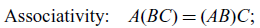 \begin{align}\text{Associativity:}&\quad A(BC) = (AB)C;\end{align}
 \begin{align}\text{Absorption:}&\quad \begin{bmatrix}A & B \end{bmatrix} (C \times D) = \begin{bmatrix} AC & BD \end{bmatrix};\end{align}
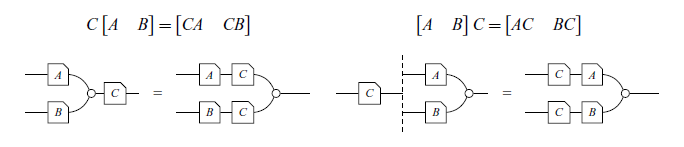
 \begin{align}\text{Divide and conquer:}&\quad \begin{bmatrix} A & B \end{bmatrix} \begin{bmatrix} C \\ D \end{bmatrix}=AC+BD.\end{align}
Laws of symmetric strict monoidal (SSM) categories. The numbering on the wires is omitted for readability.
Suppose that A, B, and C now stand for linear relations. These equations are true given the definitions of relational composition and cartesian product. The benefit from this change of perspective comes from the fact that many laws concerning matrices and subspaces become special cases of these relational laws. First, the original rules can be readily recovered by restricting A, B, and C to matrices. Now, if we let C be the subspace corresponding to the domain of B, then composing with C in (1.1) is simply taking the image. So, as it turns out, the following rule is just a special case of the associativity of relational composition:
 \begin{equation} A(Im(B)) = Im(AB).\end{equation}
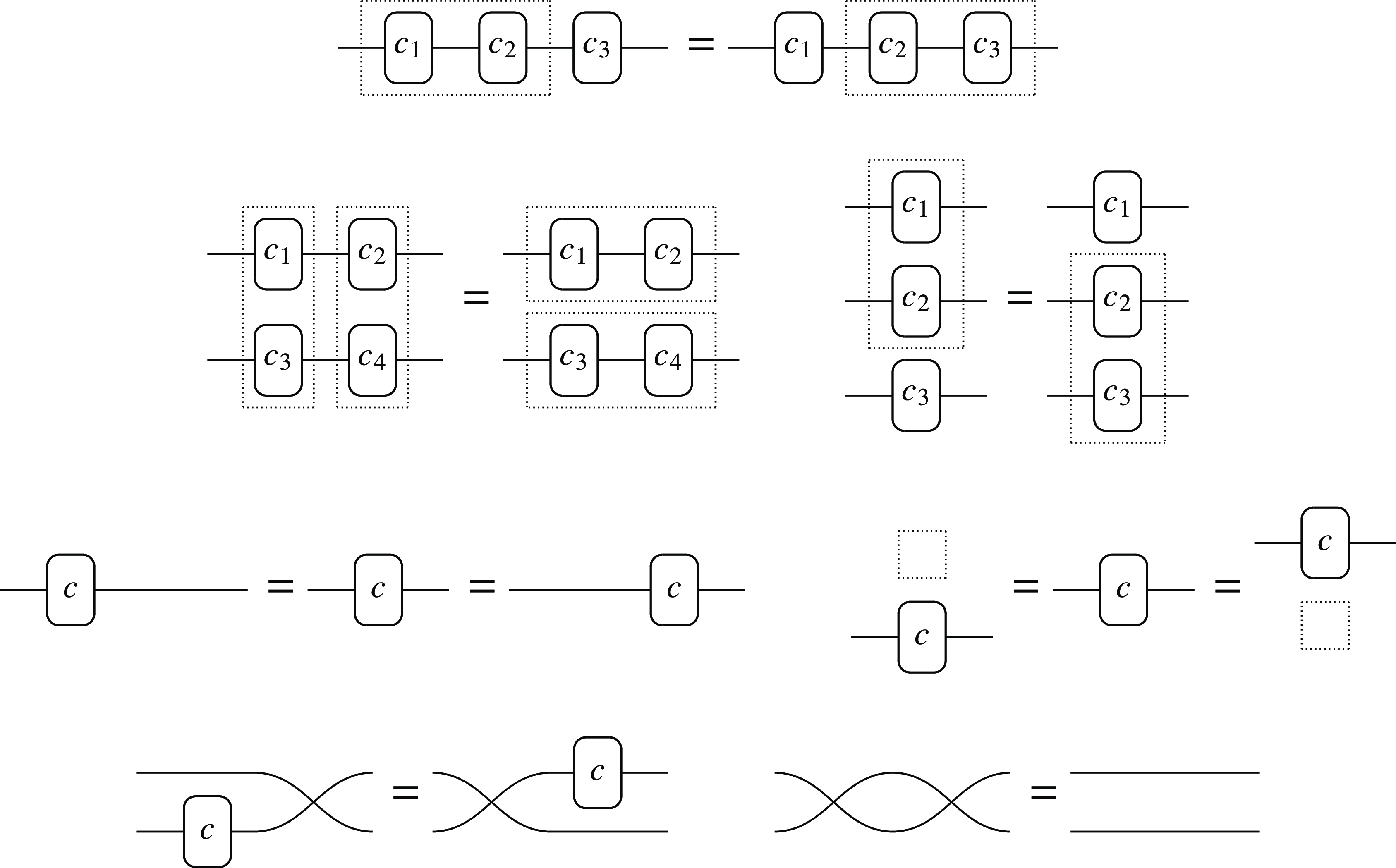
As another example, letting C and D in (1.3) be the domains of A and B respectively, we get the following common rule about the image of blocked matrices:
 \begin{equation} Im(\begin{bmatrix} A & B\end{bmatrix}) = Im(A) + Im(B).\end{equation}
Other common rules involving matrices and subspaces can also be attained via simple instantiation. This flexibility allows for calculational proofs in which both concepts are mixed together. A good example is the Zassenhaus algorithm, a method to find both the intersection and sum of two subspaces given their bases. As a proof of concept, this algorithm is verified in Section 3.2 in a point-free calculational manner.
The benefits are not restricted to verification proofs. It is well known that relational algebra is effective for point-free program derivation (Bird & De Moor, Reference Bird and De Moor1996). Thus, it is natural to expect that linear relations will play a similar role in regard to linear algebra. We give two examples of program derivation using relational algebra in Section 4.
1.3 Problems with syntax
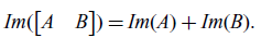
As noted before, blocked matrix notation is one of the key ingredients that allows an equational presentation of the laws of matrix algebra. However, the downside of such a choice is the loss of type information. For instance, many linear algebra students would probably need to think about the dimensions of A, B, and C to decide which of the following two equations is correct.
 \begin{equation} C \begin{bmatrix} A & B \end{bmatrix} = \begin{bmatrix} CA & CB \end{bmatrix} \text{ or } \begin{bmatrix} A & B \end{bmatrix}C = \begin{bmatrix} AC & BC \end{bmatrix}?\end{equation}
One way to solve this problem is through the use of string diagrams. As noted by Hinze & Marsden (Reference Hinze and Marsden2023), these are well-known objects in the category theory community able to allow equational reasoning without loss of type information. In a recent work, Paixão et al. (Reference Paixão, Rufino and Sobociński2022) make use of a graphical syntax for linear algebra, which uses string diagrams, known as GLA to present the laws of linear relations in an equational manner. As shown in Table 1 (the reader is not expected to fully understand the diagrams yet), type checking (1.6) in GLA amounts to checking whether the wires connect.
Type checking in GLA. The wires of the diagram on the right do not connect.
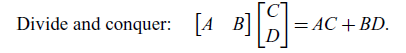
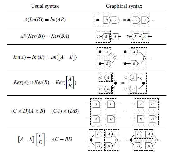
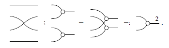
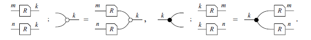
In our case, string diagrams also implicitly handle some non-trivial rules in the usual syntax, just as is commonly done with associativity by ignoring parentheses. As a simple example, below is the associativity law in graphical syntax, with the dotted lines simulating parenthesization. Table 2 exemplifies how other 6 rules are also handled implicitly by the graphical language.
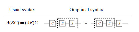
Implicit rules. The dotted lines represent parenthesization.
Dictionary of notations (Part 1).
Dictionary of notations (Part 2).
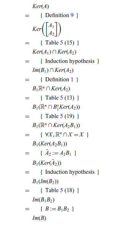
In Section 3, we employ GLA to construct proofs through verification. Two algorithms are explored: an algorithm for finding fundamental bases for the subspaces of a matrix (Beezer, Reference Beezer2014) and the Zassenhaus algorithm (Fischer, Reference Fischer2012).
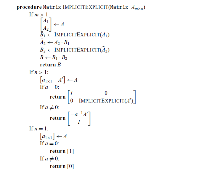
In Section 4, we utilize GLA for program derivation. Two additional examples will be presented: calculating the right inverse of a wide triangular matrix and switching from implicit to explicit basis (solving a homogeneous linear system). The pseudocode for each algorithm (which will be a systematic translation of the proof steps) will be provided. Lastly, a proof of a result concerning the duality between Gaussian elimination and the exchange lemma will also be presented (Barańczuk & Szydło, Reference Barańczuk and Szydło2021).
2 Graphical linear algebra
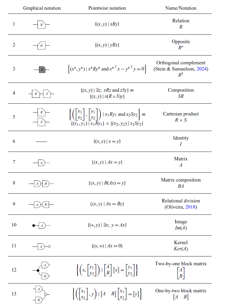
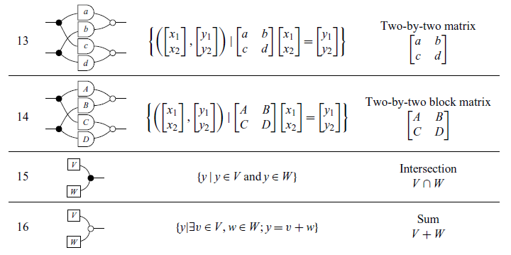
Three notations are used in this paper. The pointwise notation concerns fundamental mathematical explanations with notation of sets. The classical notation refers to terms commonly used in linear algebra such as image, kernel and block matrices. The graphical notation refers to the 2-dimensional diagrammatical notation used in GLA and will be the main focus of this section. We will briefly introduce it to the reader and show (Tables 3 and 4) how it can be translated into the other two.
Proofs in this context will make use of the diagrammatic language, in which the main ingredients are mathematical objects called string diagrams. This section explains how diagrams are constructed and outlines the structures of how to manipulate and reason with them. These diagrams are an instance of a particular class of string diagrams, which are well known to characterize the arrows of free strict monoidal categories (Selinger, Reference Selinger2010). They are, therefore, rigorous mathematical objects.
2.1 Graphical syntax
This section will present the equational theory of interacting Hopf algebras (Zanasi, Reference Zanasi2015) from which graphical linear algebra is based upon (Baez & Erbele, Reference Baez and Erbele2015; Bonchi et al., Reference Bonchi, Holland, Pavlovic and Sobocinski2017). It has been applied (and adapted) in a series of papers (Bonchi et al., Reference Bonchi, Sobociński and Zanasi2014, Reference Bonchi, Sobocinski and Zanasi2015, Reference Bonchi, Holland, Pavlovic and Sobocinski2017, Reference Bonchi, Piedeleu, Sobociński and Zanasi2019) to model signal flow graphs, Petri nets and non-passive electrical circuits. In this paper, however, the aim is to elucidate its status as a notation for linear algebra.
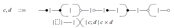
The graphical syntax is built from a series of initial diagrams (or symbols) called generators, shown in (2.1); diagrams can be combined according to two rules ( $;$
and
$;$
and $\times$
) to form bigger diagrams. Semantically, each diagram canonically represents a linear relation (this will be better explained in Section 2.2), and the rules
$\times$
) to form bigger diagrams. Semantically, each diagram canonically represents a linear relation (this will be better explained in Section 2.2), and the rules $;$
and
$;$
and $\times$
in diagrammatic notation correspond, respectively, to relational composition and cartesian product, as in Definition 2.
$\times$
in diagrammatic notation correspond, respectively, to relational composition and cartesian product, as in Definition 2.
We use
![]() to denote a generic diagram with m wires on the left and n wires on the right (the chamfered edge on the right is necessary because eventually we will need to start “flipping diagrams horizontally”, so it is important to retain directional information).
to denote a generic diagram with m wires on the left and n wires on the right (the chamfered edge on the right is necessary because eventually we will need to start “flipping diagrams horizontally”, so it is important to retain directional information).
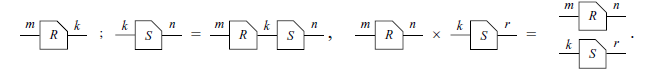
Definition 5 (Composing diagrams). The operations ; and × correspond to, respectively, attaching diagrams horizontally and vertically.
Notice that, similar to relational composition, to compute
![]() , R and S have to be compatible: the number of right-wires of R must be the same as the number of left-wires of S.
, R and S have to be compatible: the number of right-wires of R must be the same as the number of left-wires of S.
Example 2. The composition
![]() is ill-typed because the diagrams are incompatible (the first has one right-wire, whereas the second has two left-wires). The composition below, however, is valid.
is ill-typed because the diagrams are incompatible (the first has one right-wire, whereas the second has two left-wires). The composition below, however, is valid.
Example 3. The operation $\times$
corresponds to stacking diagrams vertically. It can always be performed regardless of compatibility conditions.
$\times$
corresponds to stacking diagrams vertically. It can always be performed regardless of compatibility conditions.
Example 4. Here is a more complicated example of composition.
The last example above showcases a method of combining two
![]() diagrams into a bigger one which we named
diagrams into a bigger one which we named
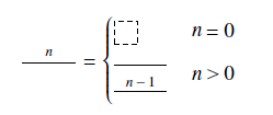
![]() . This process can be continued inductively for any number of steps, forming what we call a generalized generator, written
. This process can be continued inductively for any number of steps, forming what we call a generalized generator, written
![]() , for any
, for any $n \in \mathbb{N}$
. There are analogous constructions for each generator, as defined below.
$n \in \mathbb{N}$
. There are analogous constructions for each generator, as defined below.
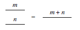
Definition 6 (Generalized generators).
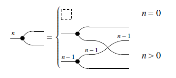
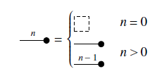
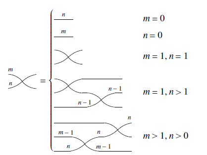
The constructions for
 and
and
![]() are what one might expect. For example,
are what one might expect. For example,
![]() is the same as
is the same as
![]() , but swapping the colors from black to white in the inductive definition. Similarly,
, but swapping the colors from black to white in the inductive definition. Similarly,
![]() is the same as
is the same as
![]() but flipping the diagrams horizontally. This sort of double-symmetry (color-swapping and horizontal-flipping) is recurrent in GLA. For instance, the Theorem below is stated only for
but flipping the diagrams horizontally. This sort of double-symmetry (color-swapping and horizontal-flipping) is recurrent in GLA. For instance, the Theorem below is stated only for
![]() and
and
![]() , but the corresponding properties for the other generators can be readily guessed correctly.
, but the corresponding properties for the other generators can be readily guessed correctly.
Theorem 1. The types defined in Definition 6 are closed by the following operations.
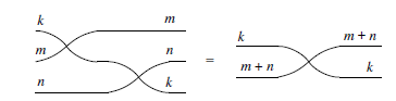
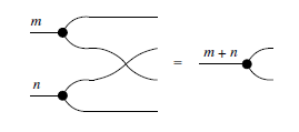
These higher-order structures help simplify notation, especially when defining certain types of diagrams inductively, like matrices (see Definition 9).
Example 5. Here’s an example of how generalized generators compose with other diagrams.
By abuse of notation, we often omit the numbering on the wires when they are irrelevant or can be inferred from the given data.
2.1.1 Symmetric strict monoidal categories
Raw terms are quotiented with respect to the laws of symmetric strict monoidal (SSM) categories, summarized in Figure 1. We omit the (well-known) details (Selinger, Reference Selinger2010) here and mention only that this amounts to eschewing the need for “dotted line boxes” and ensuring that diagrams with the same topological connectivity are equated.
2.2 Translating graphical notation to pointwise notation
In the graphical notation, each diagram semantically corresponds to a linear relation. The translation of diagrams to pointwise notation is compositional and translates their semantic meaning – the meaning of a compound diagram is calculated from the meanings of its sub-diagrams. Here there is a connection with relational algebra, the two operations of diagram composition are mapped to the standard ways of composing relations: relational composition and cartesian product. In fact, the translation of diagrams to pointwise notation can be viewed as a functor from the category of diagrams to the category of linear relations over $\mathbb{R}$
. Given that all diagrams are built from composing smaller diagrams, it suffices to show how to translate the generators.
$\mathbb{R}$
. Given that all diagrams are built from composing smaller diagrams, it suffices to show how to translate the generators.
The generators
![]() and
and
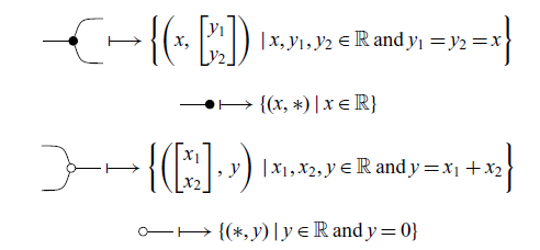
![]() are, respectively, the opposite of the relations above, as hinted by the symmetric graphical syntax. Its interpretation in pointwise notation is therefore trivial.
are, respectively, the opposite of the relations above, as hinted by the symmetric graphical syntax. Its interpretation in pointwise notation is therefore trivial.
Intuitively, the black ball in diagrams refers to copying and discarding – indeed
![]() is copy and
is copy and
![]() is discard. Meanwhile, the white ball refers to addition in
is discard. Meanwhile, the white ball refers to addition in $\mathbb{R}$
– indeed
$\mathbb{R}$
– indeed
 is add and
![]() is zero.
is zero.
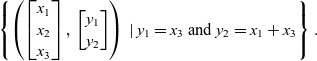
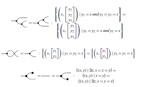
Example 6. Here’s an example of how to translate a more complicated diagram. The intuitive way to think about diagrams is like a series of logical gates, where the input starts on the left and flows to the right via the wires. In the image below we include some variable names $x_1, x_2, x_3, y_1, y_2$
(which are not wire numberings) to aid comprehension.
$x_1, x_2, x_3, y_1, y_2$
(which are not wire numberings) to aid comprehension.
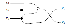
By visualizing the $x_i$
’s flowing to the right, we can see
$x_i$
’s flowing to the right, we can see $x_2$
is discarded and
$x_2$
is discarded and $x_3$
is copied. One of the copies is passed to
$x_3$
is copied. One of the copies is passed to $y_1$
while the other is added with
$y_1$
while the other is added with $x_1$
to form
$x_1$
to form $y_2$
. So
$y_2$
. So $y_1 = x_3$
and
$y_1 = x_3$
and $y_2 = x_1 + x_3$
. Thus, written in pointwise notation this diagram corresponds to the relation
$y_2 = x_1 + x_3$
. Thus, written in pointwise notation this diagram corresponds to the relation
 $$\left\{\left(\begin{bmatrix}x_1\\x_2\\x_3 \end{bmatrix},\, \begin{bmatrix}y_1\\y_2 \end{bmatrix}\right) \in \mathbb{R}^3 \times \mathbb{R}^2 \;|\; y_1=x_3 \text{ and } y_2=x_1+x_3 \right\}.$$
For the purpose of simplifying the notation, sometimes in this paper, the inclusion “ $\in \mathbb{R}^3 \times \mathbb{R}^2$
” will be omitted and diagrams such as the one presented above will be written in pointwise notation as follows.
$\in \mathbb{R}^3 \times \mathbb{R}^2$
” will be omitted and diagrams such as the one presented above will be written in pointwise notation as follows.
 $$\left\{\left(\begin{bmatrix}x_1\\x_2\\x_3 \end{bmatrix},\, \begin{bmatrix}y_1\\y_2 \end{bmatrix}\right) \;|\; y_1=x_3 \text{ and } y_2=x_1+x_3\right\}.$$
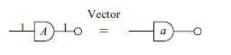
2.3 Scalars, matrices and other constructions
We’ve seen that linear transformation (or linear maps) can be thought of as special cases of linear relations. This section explains some basic types of maps which will be used throughout the paper. The most basic linear map is scalar multiplication: given $a \in \mathbb{R}$
, one can define the map
$a \in \mathbb{R}$
, one can define the map $[a] : \mathbb{R} \rightarrow \mathbb{R}$
given by
$[a] : \mathbb{R} \rightarrow \mathbb{R}$
given by $x \mapsto ax$
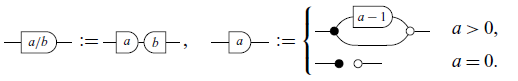
. In diagrammatic notation, we write it as the
$x \mapsto ax$
. In diagrammatic notation, we write it as the $1 \times 1$
curved diagram
$1 \times 1$
curved diagram
![]() , always with a lowercase letter. Semantically
, always with a lowercase letter. Semantically
If we restrict ourselves to scalars in $\mathbb{Q}$
, any scalar multiplication can be built inductively from the generators. Below we define diagrammatically the maps [q] for
$\mathbb{Q}$
, any scalar multiplication can be built inductively from the generators. Below we define diagrammatically the maps [q] for $0 \leq q \in \mathbb{Q}$
.
$0 \leq q \in \mathbb{Q}$
.
Definition 7 (Scalars in
$\mathbb{Q}$
). For $a, b \in \mathbb{N}, b \ne 0,$
The maps corresponding to negative numbers can also be built, but defining $[-1]$
is somewhat confusing so we won’t delve further into this discussion. For more information, see Sobociński (Reference Sobociński2015). As a last note on scalars, if we work under an uncountable field such as
$[-1]$
is somewhat confusing so we won’t delve further into this discussion. For more information, see Sobociński (Reference Sobociński2015). As a last note on scalars, if we work under an uncountable field such as $\mathbb{R}$
, there is no way to build all scalars from the generators for cardinality reasons. Hence, formally, one needs an uncountable amount of new generators
$\mathbb{R}$
, there is no way to build all scalars from the generators for cardinality reasons. Hence, formally, one needs an uncountable amount of new generators
![]() with
with $a \in \mathbb{R}$
.
$a \in \mathbb{R}$
.
Aside from scalars, another important construction is that of a matrix. In the graphical language, a matrix is considered a linear transformation built inductively from the generators in a way that resembles the column-by-column construction of classical block matrices. More concretely, here’s an inductive definition of a matrix in the usual sense.
Definition 8 (Matrix, column-by-column).
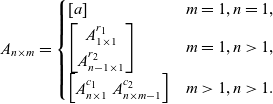 \begin{equation*} A_{n \times m} = \begin{cases} [a] & m=1,n=1,\\ \begin{bmatrix}A^{r_1}_{1 \times 1} \\ A^{r_2}_{n-1 \times 1} \end{bmatrix} & m=1,n>1,\\ \begin{bmatrix}A^{c_1}_{n \times 1} & A^{c_2}_{n \times m-1} \end{bmatrix} & m>1,n>1. \end{cases} \end{equation*}
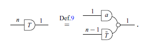
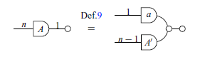
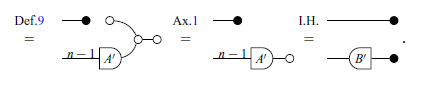
We can mimic this definition in diagrammatic notation.
Definition 9 (Matrix in GLA).
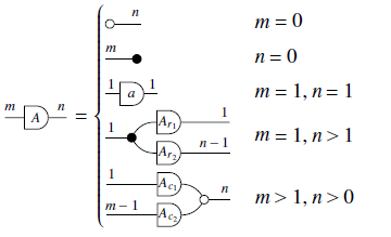
Except for the two first cases, which account for diagrams with zero left/right wires, the different cases in the graphical definition are exactly the different cases in the usual, column-by-column definition. Notice that we write a matrix
![]() as a curved diagram, in order to distinguish them from ordinary relations. We write a matrix with lowercase letters if and only if it is a
as a curved diagram, in order to distinguish them from ordinary relations. We write a matrix with lowercase letters if and only if it is a $1 \times 1$
matrix, i.e. a scalar.
$1 \times 1$
matrix, i.e. a scalar.
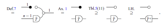
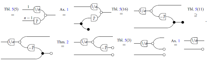
Example 7. The triangular matrix $\begin{bmatrix}2 & 3\\ 0 & 1\end{bmatrix}$
can be written in graphical syntax as
$\begin{bmatrix}2 & 3\\ 0 & 1\end{bmatrix}$
can be written in graphical syntax as
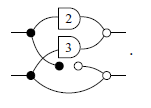
However, this diagram presents an inefficient coding for the given matrix and can be simplified based on the Axioms and Theorems that will be exposed below.
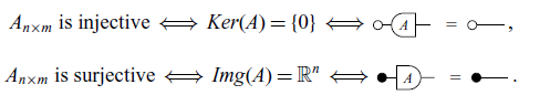
We also mentioned in the Introduction that subspaces are special cases of linear relations. They can be thought of as relations $R \subseteq V \times W$
where
$R \subseteq V \times W$
where $V = \{*\}$
is the zero-dimensional space. In diagrammatic notation, these correspond to the diagrams with 0 wires on the left. We write them as
$V = \{*\}$
is the zero-dimensional space. In diagrammatic notation, these correspond to the diagrams with 0 wires on the left. We write them as
![]() . Given a matrix
. Given a matrix $A_{n \times m}$
, some familiar subspaces are
$A_{n \times m}$
, some familiar subspaces are
![]() (the image of A) and
(the image of A) and
![]() (the kernel of A). With these, we can define surjectivity and injectivity graphically.
(the kernel of A). With these, we can define surjectivity and injectivity graphically.
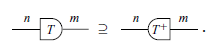
In fact, as a side note, linear transformations can be defined as linear relations satisfying
![]() and
and
![]() . If these equations hold, we say the relation R is, respectively, single-valued and total (see Definition 11). It is not difficult to prove, under this definition, that matrices are linear transformations.
. If these equations hold, we say the relation R is, respectively, single-valued and total (see Definition 11). It is not difficult to prove, under this definition, that matrices are linear transformations.
Tables 3 and 4 showcase some other constructions that will appear throughout the paper. Some new symbols are introduced: R,S denote mathematical relations; A,B,C,D represent matrices (linear transformations); a,b,c,d are real numbers; and V,W are subspaces. For simplicity, sometimes we write the expression $(x, y) \in R$
as xRy. It is worth noting that the dagger symbol
$(x, y) \in R$
as xRy. It is worth noting that the dagger symbol $R^\dagger$
used below is not the dagger that appears in the context of dagger categories. A proper inductive definition of the dagger is given in Definition 10, and it corresponds to the intuitive notion of color-swapping, i.e. transforming white nodes into black nodes and vice-versa.
$R^\dagger$
used below is not the dagger that appears in the context of dagger categories. A proper inductive definition of the dagger is given in Definition 10, and it corresponds to the intuitive notion of color-swapping, i.e. transforming white nodes into black nodes and vice-versa.
2.4 Diagrammatic reasoning
Now we present the axioms and theorems that will be used for the remainder of the paper. It is worth noting that here there are just three of the axioms of GLA. The complete presentation of the axioms can be found at Paixão et al. (Reference Paixão, Rufino and Sobociński2022). Most proofs in this section will be omitted as they are not the focus of this work, but can be found in the same reference. The axioms and theorems are inspired by the notion of an Abelian bicategory as defined by Carboni & Walters (Reference Carboni and Walters1987). Here, two combinations of diagrams that play an important role are bialgebras and special Frobenius algebras (respectively, Theorems 2 and 3). As explained by Lack (Reference Lack2004), these are two canonical ways in which monoids and comonoids can interact.
Axiom 1 (Commutative comonoid). The copy diagram satisfies the equations of commutative comonoids, that is, associativity, commutativity and unitality, as given below:
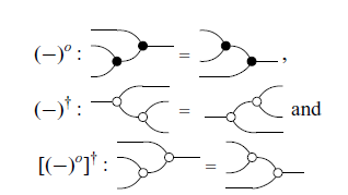
In graphical notation, the diagrams are closed under two symmetries: the “Mirror-Image” and the “Color-Swap”.
Definition 10 (Mirror-Image and Color-Swap). Mirror-Image (denoted by $(-)^o$
) and Color-Swap (denoted by
$(-)^o$
) and Color-Swap (denoted by $(-)^\dagger$
) are defined on the generators in the obvious way and extended recursively as follows:
$(-)^\dagger$
) are defined on the generators in the obvious way and extended recursively as follows:
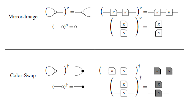
Axiom 2 (Symmetries). We have the equivalences $R^o \subseteq S \iff R \subseteq S^o$
, i.e. in diagrams
$R^o \subseteq S \iff R \subseteq S^o$
, i.e. in diagrams
and $R^\dagger \subseteq S \iff R \supseteq S^\dagger$
, or in diagrams
$R^\dagger \subseteq S \iff R \supseteq S^\dagger$
, or in diagrams
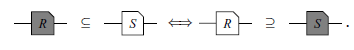
In Axiom 2,
![]() represents the diagram with inverted colors, where black circles turn white, and vice versa. Axiom 2 denotes a particularly relevant advantage of graphical notation. As an example, consider the axiom below.
represents the diagram with inverted colors, where black circles turn white, and vice versa. Axiom 2 denotes a particularly relevant advantage of graphical notation. As an example, consider the axiom below.
Axiom 3 (Discard).
Applying Axiom 2 to Axiom 3, we can assert that:

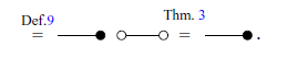
For equalities, this becomes even simpler. It can be assumed that each diagram has three other versions: the ‘mirror image,’ the ‘color swap,’ and both together. If an equation is valid, its other three versions are also valid. For example, from Axiom 1, it is known that the equality
 is true. Therefore, by Axiom 2:
are also true. When a result is proven, it will be assumed that the other three versions are also true, just referencing the original result. For example, all of the above statements will be denoted simply by Axiom 1.

White and black diagrams act as bialgebras when they interact. This can be summarized by the following equations.
Theorem 2. (Bialgebra).
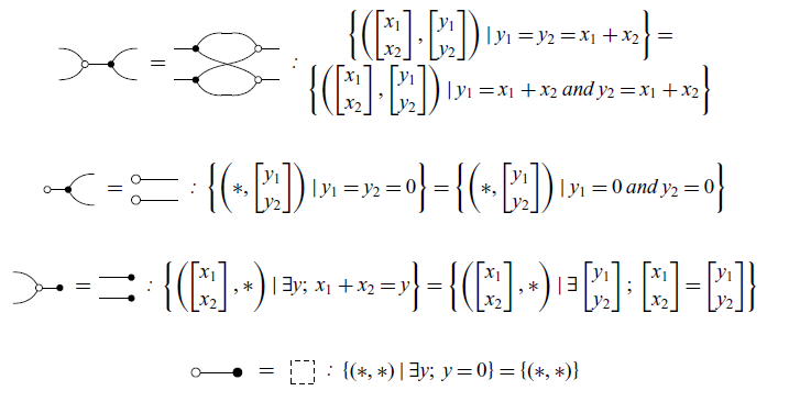
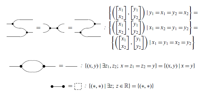
The white and black diagrams interact according to the rules of bialgebras. On the other hand, individually the white and black structures interact as (extraspecial) Frobenius algebras.
Theorem 3. (Frobenius Algebra). The following equations hold:
We now define the following important properties about linear relations.
Definition 11 (Types of relations). The R relation is called:
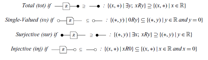
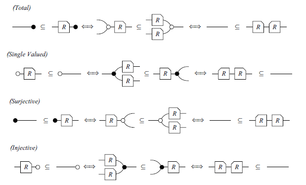
Definition 11 has equivalent statements, summarised in the Theorem below:
Theorem 4. For every relation R, the following statements are equivalent:
Remark. A diagram is a map if it is total and single-valued. Also, a diagram is a Co-map if it is injective and surjective. In particular, a matrix
![]() is a Map.
is a Map.
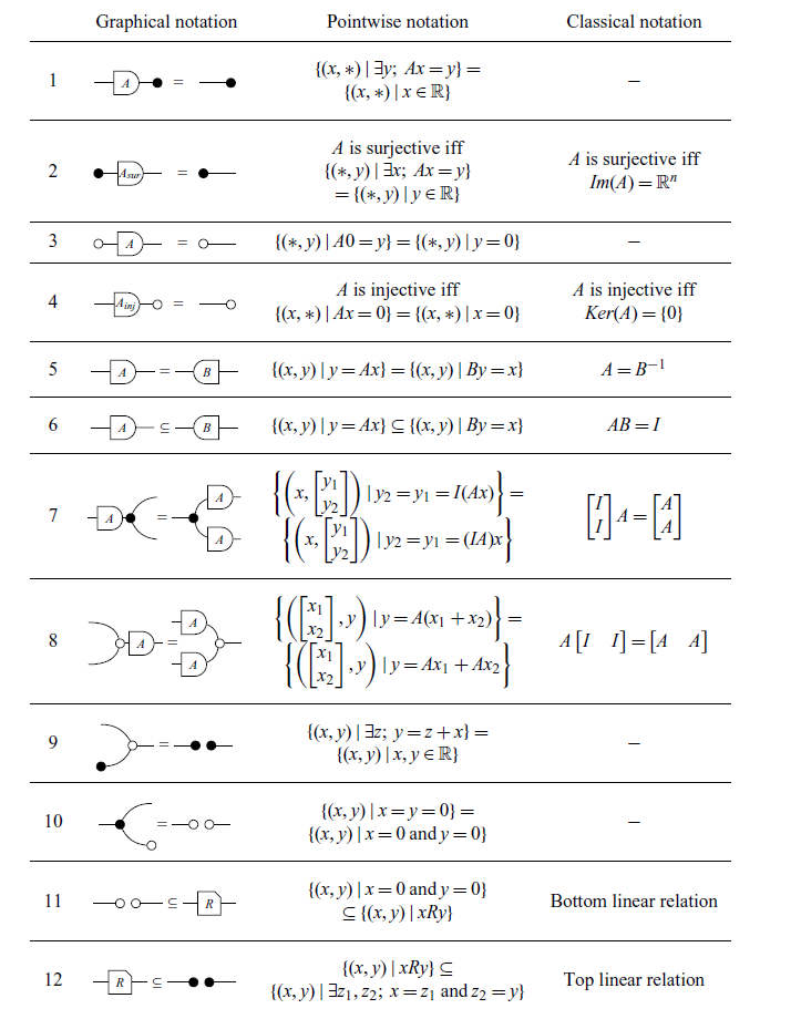
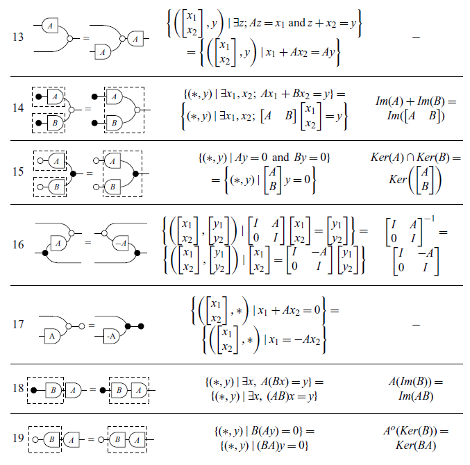
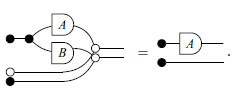
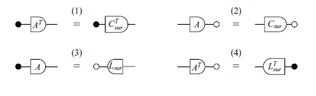
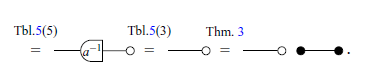
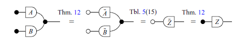
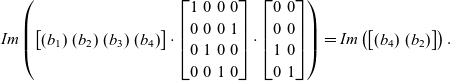
The other theorems relevant to this paper are summarized in Table 5. It is worth mentioning that the translations in pointwise notation presented are well-known theorems in linear algebra, which can be easily verified in a classical textbook, for example (Axler, Reference Axler1997; Strang, Reference Strang2009).
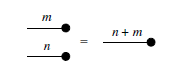
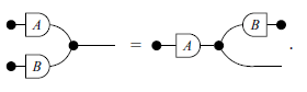
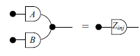
In Table 5, the dotted lines in some of the rows have no syntactic meaning and are included solely to visually illustrate the two ways in which the diagram in question can be semantically interpreted as it was done in introduction. For instance, the equation in row 18, which is a theorem in classical notation, implicitly holds true in the graphical syntax.
Theorems, presented in the three different notations (Part 1).
Theorems, presented in the three different notations (Part 2).
Lastly, we state three additional Lemmas which will be useful in the next sections. Lemmas 1 and 2 will be used in the proof of the Zassenhaus’ algorithm (Theorem 9), while Lemma 3 will appear later, in the proof of the Exchange Lemma (Theorem 16). The reason for providing specific proofs of these three lemmas is to use them as examples of how Tables 3 and 5 can help in translating proofs from graphical notation into two other notations.
Lemma 1.
Proof
Lemma 2.
Proof
Lemma 3.
Proof
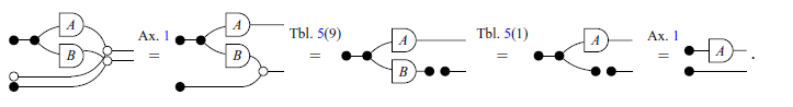
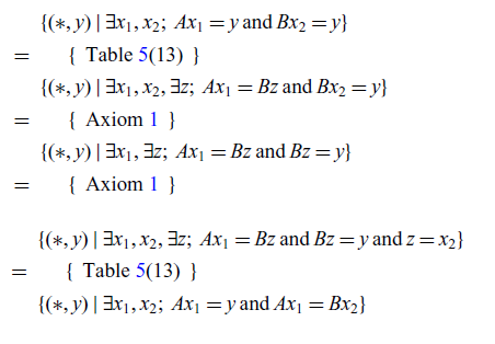
We can almost immediately obtain the same proofs (Lemmas 1, 2 and 3) in pointwise notation by systematically translating each step according to the Tables 3 and 5.
Lemma 4. (Lemma 1 in pointwise version).
 $$\left \{{ (*,y) \mid \exists} x_1,x_2;\; Ax_1=y \;\text{and}\;Bx_2=y \right \}=\left \{{ (*,y) \mid \exists} x_1,x_2;\; Ax_1=y \;\text{and}\;Ax_1=Bx_2 \right \}$$
Proof
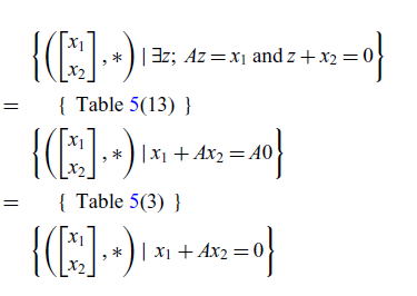
Lemma 5. (Lemma 2 in pointwise version). Let A be a matrix, then
 $$\left \{ \left ( \begin{bmatrix}x_1 \\x_2\end{bmatrix}, *\right ) \mid \exists z;\;Az=x_1\;\text{and}\;z+x_2=0 \right \}=\left \{ \left ( \begin{bmatrix}x_1 \\x_2\end{bmatrix}, *\right ) \mid x_1+Ax_2=0 \right \}$$
Proof
Lemma 6. (Lemma 3 in pointwise notation) Given two matrices $A_{n_1 \times m}$
and
$A_{n_1 \times m}$
and $B_{n_2 \times m}$
, then
$B_{n_2 \times m}$
, then
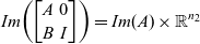 $$Im{\left (\begin{bmatrix}A & 0\\B & I\end{bmatrix} \right )}=Im{(A)} \times\mathbb{R}^{n_2} $$
Proof
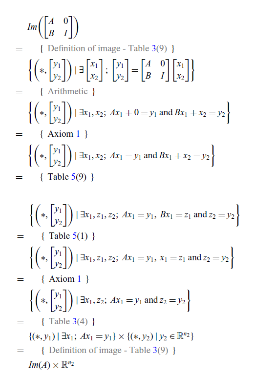
Note that in the proof of Lemma 6, some steps (gray letters) are needed in addition to those used in the graphical version (Lemma 3). In fact, this is quite common. Informally speaking, proofs in GLA often have fewer steps than their classical counterparts. There are two main reasons for this. The first is that, as seen in rows 14, 15, and 18 of Table 5, some non-trivial rules in the usual notation become implicitly true in GLA. The second is that the definitions of kernel and image do not require specific terminology; instead, they can be built from the pre-established fundamental symbols (zero, discard, and matrices).
3 Verification proofs in GLA
This section presents two distinct verification proofs in GLA about linear subspaces. The first one is an introductory example from which the reader can draw intuition. Thus, in this case, the same proof will be written in all three types of notation. The second example will be compared to the widely available Wikipedia proof.
3.1 Introductory example: finding the fundamental subspaces
Definition 12 (Fundamental Subspaces). For any matrix A, there are four fundamental subspaces: Im(A), $Im{(A^\top)}$
, Ker(A) and
$Im{(A^\top)}$
, Ker(A) and $Ker{(A^\top)}$
.
$Ker{(A^\top)}$
.
The algorithm presented by Beezer (Reference Beezer2014) determines bases for these four subspaces in a single calculation using Reduced Row Echelon Form (RREF) obtained through row operations. This algorithm can be stated as follows.
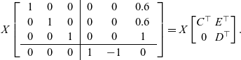
Theorem 5. (Bases for Fundamental Subspaces). For every matrix $A_{m\times n}$
, if there are surjective matrices C and L, a matrix K, and an invertible matrix X such that
$A_{m\times n}$
, if there are surjective matrices C and L, a matrix K, and an invertible matrix X such that
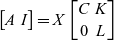 \begin{equation*} \begin{bmatrix}A & I\end{bmatrix}=X\begin{bmatrix}C & K\\0 & L\end{bmatrix}\end{equation*}
the following equalities hold.
-
1.
$Im{(A^\top)}=Im{(C^\top)}$
, -
2.
$Ker{(A)}=Ker{(C)}$
, -
3.
$Im{(A)}=Ker{(L)}$
, -
4.
$Ker{(A^\top)}=Im{(L^\top)}$
.


Example 9. Let $A= \begin{bmatrix}1 & 1 \\1 & 2 \\1 & 3\end{bmatrix}$
. Then
$A= \begin{bmatrix}1 & 1 \\1 & 2 \\1 & 3\end{bmatrix}$
. Then
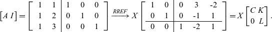
See that the equations 1, 2, 3 and 4 of Theorem 5 hold:
-
1.
$Im{(A^\top)}=\left\{ \begin{bmatrix}1 \\1\end{bmatrix},\begin{bmatrix}1 \\2\end{bmatrix} \right\}=\mathbb{R}^2$
and
$Im{(C^\top)}=\left\{ \begin{bmatrix}1 \\0\end{bmatrix},\begin{bmatrix}0 \\1\end{bmatrix} \right\}=\mathbb{R}^2$
; -
2.
$Ker{(A)}=Ker{(C)}=0$
; -
3.
$Ker{(L)}=\left\{ \begin{bmatrix}2\\1 \\0\end{bmatrix},\begin{bmatrix}-1\\0 \\1\end{bmatrix} \right\}=\mathbb{R}^3$
and
$Im{(A)}=\left\{ \begin{bmatrix}1\\1 \\1\end{bmatrix},\begin{bmatrix}1\\2 \\3\end{bmatrix} \right\}=\mathbb{R}^3$
; -
4.
$Ker{(A^\top)}=Im{(L^\top)}=\left\{ \begin{bmatrix}1\\-2 \\1\end{bmatrix} \right\}$
.


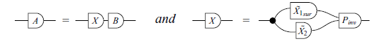
In graphical syntax, Theorem 5 takes the following form:
Theorem 6. (Bases for Fundamental Subspaces – Graphical version). For every matrix $A_{m\times n}$
, if there are surjective matrices C and L, a matrix K, and an invertible matrix X such that
$A_{m\times n}$
, if there are surjective matrices C and L, a matrix K, and an invertible matrix X such that
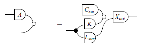
then
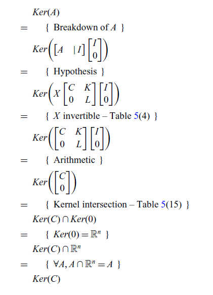
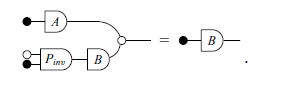
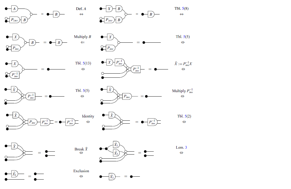
We begin by exploring the proof of items 1 and 2.
Proof of (2)
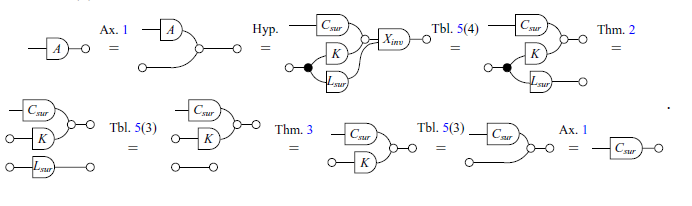
Proof of (1) It is proved by the Proof (2) and the Theorem 2.
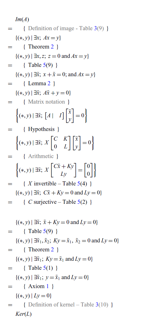
As seen in Section 2, each diagram has a semantic translation to pointwise notation. Therefore, based on the graphical proof above, we immediately obtain the following proof by translating each step systematically.
Proof of (2) [Pointwise version]
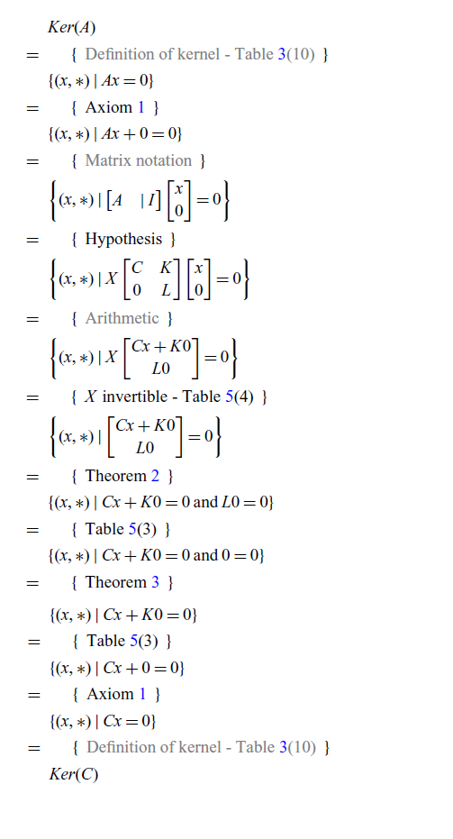
In a similar way, using Table 5 the same proof can be written in classical notation.
Proof of (2) [Classical version]
Now we prove items 3 and 4.
Proof of (3) [Graphical version]
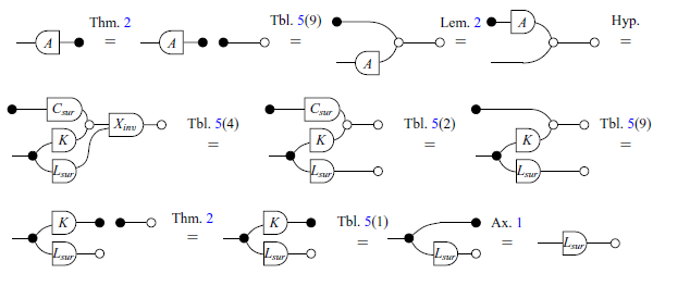
Proof of (4) [Graphical version]
It is proved by the Proof (3) and the Theorem 2.
Again, translating each step systematically, we obtain the proof in pointwise notation:
Proof of (3) [Pointwise version]
In this case, as shown in Table 5, some steps have no direct translations into classical notation. Hence, the following translation of the graphical proof relies on pointwise notation to fill in the gaps. Informally speaking, this often happens when multiple matrices interact with each other in a non-trivial way. The graphical language is expressive enough to handle these complex interactions without the need to introduce new symbols.
3.2 The Zassenhaus’ algorithm
The Zassenhaus algorithm is a well-known method that calculates a basis for the intersection and another for the sum of two subspaces of a vector space. According to Fischer (Reference Fischer2012), despite being attributed to Hans Zassenhaus (1912–1991), there is no publication of this algorithm in the mathematician’s works. However, there is a historical association regarding its application in Zassenhaus’ classic coffee grinder manufacturing company. This algorithm serves as a compelling example of how graphical syntax can be used to reason about linear subspaces.
Although there is published research exploring the Zassenhaus algorithm, the most widely available source is presented in Wikipedia contributors (2023), which describes the algorithm verbatim as presented in Appendix A.
The pointwise Wikipedia proof is using much subspace notation, has to define $\pi_1$
,
$\pi_1$
, ${\pi _{1}|}_{H}$
, has the word “obviously”, is full of indices to connect the matrices and subspaces, and uses dimension.
${\pi _{1}|}_{H}$
, has the word “obviously”, is full of indices to connect the matrices and subspaces, and uses dimension.
We begin by reformulating the algorithm as a theorem to make the assumptions clearer and write the proof in calculational style. In classical notation, the Zassenhaus algorithm, as presented by Wikipedia contributors (2023), can be summarized with the following theorem:
Theorem 7. For all subspaces A and B, if there are injective C and D, a matrix E, and invertible X, such that:
 \begin{equation*}\begin{bmatrix}A^\top & A^\top\\B^\top & 0\end{bmatrix} =X \begin{bmatrix}C^\top & E^\top \\0 & D^\top \\0 & 0\end{bmatrix}\text{,}\end{equation*}
then,
-
1.
$Im(A) \cap Im(B) = Im(D)$
-
2.
$Im(A) + Im(B) = Im(C)$


Example 10. Let $A=\begin{bmatrix}1 & 0 \\-1 & 0 \\0 & 1 \end{bmatrix}$
and
$A=\begin{bmatrix}1 & 0 \\-1 & 0 \\0 & 1 \end{bmatrix}$
and $B=\begin{bmatrix}5 & 0 \\0 & 5 \\-3 & -3 \end{bmatrix}$
. Then
$B=\begin{bmatrix}5 & 0 \\0 & 5 \\-3 & -3 \end{bmatrix}$
. Then
Therefore
-
1.
$Im(A) \cap Im(B) = Im(D) = \left\{ \begin{bmatrix}1 \\-1 \\ 0\end{bmatrix}\right\}$
-
2.
$Im(A) + Im(B) = Im(C) = \left\{ \begin{bmatrix}1 \\0 \\ 0\end{bmatrix},\begin{bmatrix}0 \\1 \\ 0\end{bmatrix},\begin{bmatrix}0 \\0 \\ 1\end{bmatrix}\right\}=\mathbb{R}^3$


Note that the matrices are transposed because Wikipedia contributors (2023) formulate the matrix in blocks with row vectors. To facilitate notation, we will consider the block matrix in the following equivalent (transposed) form.
Theorem 8. (Zassenhaus). For all matrices A and B, if there are injective matrices C and D, a matrix E, and an invertible matrix X such that
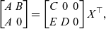 \begin{equation*}\begin{bmatrix}A & B\\A & 0\end{bmatrix} =\begin{bmatrix}C & 0 & 0 \\E & D & 0\end{bmatrix}X^\top\text{,}\end{equation*}
then
-
1.
$Im(A) \cap Im(B) = Im(D)$
, -
2.
$Im(A) + Im(B) = Im(C)$
.


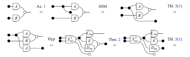
Similarly, this theorem can be expressed in graphical syntax.
Theorem 9. (Zassenhaus – Graphical version). For all matrices A and B, if there are injective matrices C and D, a matrix E, and an invertible matrix X such that
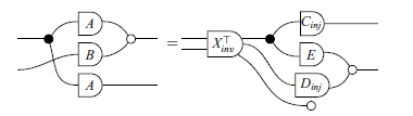
then
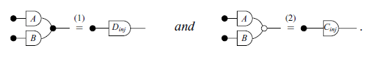
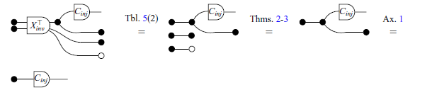
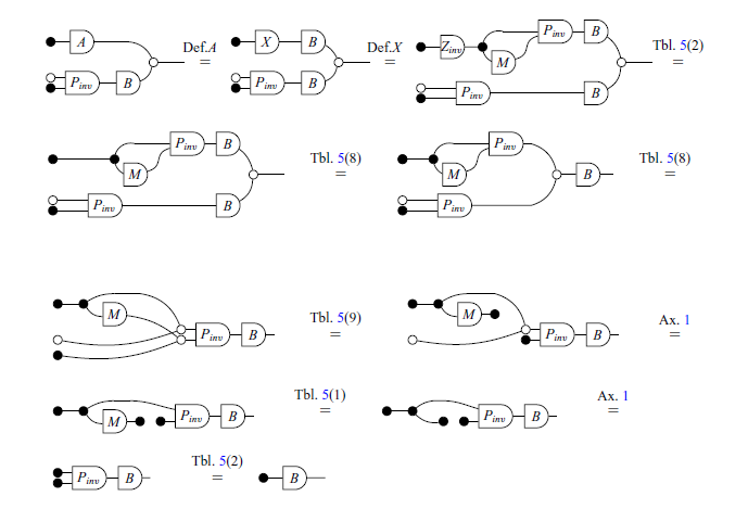
Let us rephrase the proof of the theorem using graphical syntax.
Proof of (1) [Graphical version]
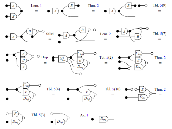
Proof of (2) [Graphical version]
See that we have achieved a completely calculational and point-free proof. Moreover, the proof in graphical syntax serves as a guide to produce a new proof in pointwise notation (Appendix B).
4 Programs and properties derivation in GLA
In this section, four main algorithms will be explored: how to find the right inverse of a wide triangular matrix, how to switch from an implicit basis description to an explicit basis description of a subspace, how to find a basis for the intersection of two subspaces and the exchange lemma. The first three algorithms are good examples of how it is possible to use graphical syntax to perform program derivations concerning linear subspaces. The last algorithm exemplifies the use of graphical syntax to derive important properties to be considered for problem-solving.
4.1 Simple example: Right inverse of a wide triangular matrix
As an introductory example, we will discuss the problem of finding the right inverse of a wide triangular matrix.
Definition 13 (Recursive Wide Triangular Matrix/Classical notation). A wide triangular matrix $T_{m \times n}$
is recursively defined as
$T_{m \times n}$
is recursively defined as
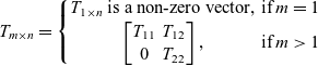 $$T_{m \times n}=\left\{\begin{matrix}T_{1 \times n}\; \text{is a non-zero vector,} & \text{if}\;m=1 \\\begin{bmatrix}T_{11} & T_{12}\\0 & T_{22}\end{bmatrix}, & \text{if}\;m>1\end{matrix}\right. $$
where $T_{12}$
is a matrix and
$T_{12}$
is a matrix and $T_{11}$
and
$T_{11}$
and $T_{22}$
are smaller wide triangular matrices.
$T_{22}$
are smaller wide triangular matrices.
This definition is almost like that of a triangular matrix, but it allows for more columns than rows. Note that it is tricky to define this matrix non-recursively. This definition leads to matrices that are surjective but not necessarily injective. In fact, every matrix constructed by the above recursive rule is surjective. Below, we present a proof by verification in classical notation.
Theorem 10. (Verification/Classical version). Let T be a wide triangular matrix, then T has a right inverse $T^+$
. In other words, there exists an
$T^+$
. In other words, there exists an $T^+$
such that
$T^+$
such that $TT^+= I$
and
$TT^+= I$
and
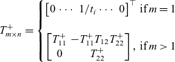 $$T_{m \times n}^+=\left\{\begin{matrix}\begin{bmatrix}0 & \cdots & 1/t_i & \cdots & 0\end{bmatrix}^\top & \text{if}\;m=1 \\ \\\begin{bmatrix} T_{11}^{+} & - T_{11}^{+} T_{12} T_{22}^{+} \\ 0 & T_{22}^{+} \end{bmatrix}, & \text{if}\;m>1\end{matrix}\right.$$
Proof The proof will be done by strong induction. First, for the base case, consider a wide triangular matrix $T_{1 \times n}=\begin{bmatrix}t_1 & t_2 & ... & t_n\end{bmatrix}$
.
$T_{1 \times n}=\begin{bmatrix}t_1 & t_2 & ... & t_n\end{bmatrix}$
.
For the inductive step, consider T in blocks as in the recursive definition.

Example 11. The matrix $T=\begin{bmatrix}3 & 2 & 3 & 4 \\0 & 5 & 2 & 1 \\\end{bmatrix}$
is wide triangular. So
$T=\begin{bmatrix}3 & 2 & 3 & 4 \\0 & 5 & 2 & 1 \\\end{bmatrix}$
is wide triangular. So $T_{11}^+=\begin{bmatrix}1/3\end{bmatrix}$
,
$T_{11}^+=\begin{bmatrix}1/3\end{bmatrix}$
, $T_{22}^+=\begin{bmatrix}1/5 & 1/2 & 1 \\ \end{bmatrix}^\top$
and
$T_{22}^+=\begin{bmatrix}1/5 & 1/2 & 1 \\ \end{bmatrix}^\top$
and
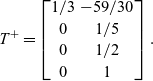 \[T^+=\begin{bmatrix}1/3 & -59/30 \\0 & 1/5 \\0 & 1/2 \\0 & 1 \\\end{bmatrix}.\]
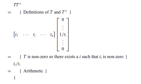
Note that $TT^+=\begin{bmatrix}1 & 0 \\0 & 1\end{bmatrix}$
. Therefore,
$TT^+=\begin{bmatrix}1 & 0 \\0 & 1\end{bmatrix}$
. Therefore, $T^+$
is the right inverse of T.
$T^+$
is the right inverse of T.
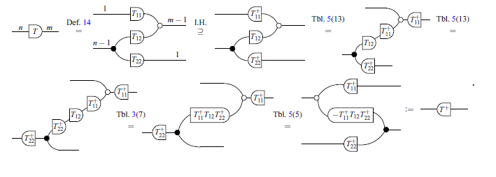
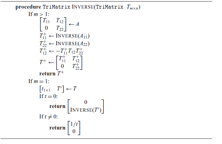
The disadvantage of this method has already been pointed out. One has to provide a candidate for the right inverse prior to the verification. In order to derive the inverse, we first reformulate the problem in GLA.
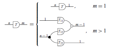
Definition 14 (Recursive Wide Triangular Matrix/Graphical version). A triangular wide matrix $T_{m \times n}$
is defined recursively by
$T_{m \times n}$
is defined recursively by
where $T_{11}$
and
$T_{11}$
and $T_{22}$
are smaller wide triangular matrices.
$T_{22}$
are smaller wide triangular matrices.
Theorem 11. (Derivation/Graphical version). Let T be a wide triangular matrix. There exists a wide triangular matrix $T^+$
such that:
$T^+$
such that:
Proof The proof will be done by induction. For the base case ( $T_{1 \times n}$
) we have
$T_{1 \times n}$
) we have
If $a = 0$
,
$a = 0$
,
If $a \neq 0$
,
$a \neq 0$
,
For the inductive step, consider
![]() in blocks as in the recursive Definition 14.
in blocks as in the recursive Definition 14.
This automatically leads to a computer implementation (by simply translating each step of the proof into the pseudocode).
Right Inverse Triangular
4.2 Switching from implicit to explicit basis
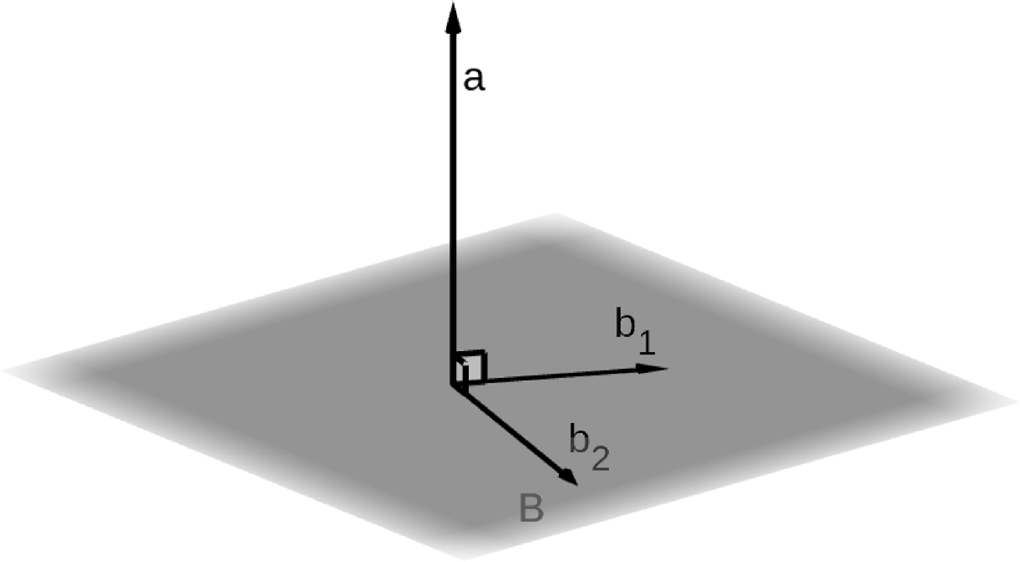
A subspace can always be represented by implicit and explicit bases, as presented by Zanasi (Reference Zanasi2015). Let $B \subseteq \mathbb{R}^n$
be a subspace, and let
$B \subseteq \mathbb{R}^n$
be a subspace, and let $a_1,a_2,...,a_m$
be vectors orthogonal to B, as depicted in Figure 2. An implicit basis of this subspace is given by
$a_1,a_2,...,a_m$
be vectors orthogonal to B, as depicted in Figure 2. An implicit basis of this subspace is given by
 \[\left\{ x \mid x\perp a_1, x\perp a_2,\ldots, x\perp a_m\right\}=\left\{ x \mid a_1^\top x=0, a_2^\top x=0,\ldots, a_m^\top x=0\right\}=\left\{ x \mid A^\top x=0 \right\}.\]
On the other hand, given $b_1, b_2,\ldots,b_r \in B$
, an explicit basis of B is given by
$b_1, b_2,\ldots,b_r \in B$
, an explicit basis of B is given by
 \[\left\{ x \mid \exists c_1, c_2, \cdots c_n \in \mathbb{R};\;c_1b_1 + c_2b_2 +\cdots+c_rb_r=x \right\}=\left\{ x \mid \exists c \in \mathbb{R}^n;\;Bc=x \right\}.\]
Geometric representation of the implicit and explicit bases of the B subspace.
Example 12. The subspace orthogonal to the vector $a=\begin{bmatrix}1 & 2 & 3\end{bmatrix}^\top$
can also be generated by the column vectors of the matrix
$a=\begin{bmatrix}1 & 2 & 3\end{bmatrix}^\top$
can also be generated by the column vectors of the matrix $B=\begin{bmatrix}-2 & -3 \\1 & 0 \\0 & 1\end{bmatrix}$
.
$B=\begin{bmatrix}-2 & -3 \\1 & 0 \\0 & 1\end{bmatrix}$
.
This can be denoted by the following theorem and proved recursively in graphical syntax.
Theorem 12. (Switch from implicit to explicit basis). For every matrix $A_{m\times n}$
, there exists a matrix
$A_{m\times n}$
, there exists a matrix $B_{n\times r}$
such that
$B_{n\times r}$
such that
Proof The proof will be done by induction. For the base case, if $m=1$
, there are two cases: Case 1 (
$m=1$
, there are two cases: Case 1 ( $n=1$
):
$n=1$
):
If $a=0$
,
$a=0$
,
If $a\neq 0$
,
$a\neq 0$
,
Case 2 ( $n>1$
):
$n>1$
):
If $a=0$
,
$a=0$
,
If $a\neq 0$
,
$a\neq 0$
,

Inductive step:

The inductive step can of course be written in classical linear algebra notation mixed with relational algebra notation as follows.
Proof [Classical version]
Furthermore this proof provides a nice recursive algorithm presented below:
Implicit to Explicit Basis
4.2.1 Calculating a basis for the intersection
The example of section (4.2) motivates the next Theorem, in which we want to build a basis for the intersection of two subspaces.
Example 13. As shown in Example 10, a basis for the intersection of the images of the subspaces $A=\begin{bmatrix}1 & 0 \\-1 & 0 \\0 & 1 \end{bmatrix}$
and
$A=\begin{bmatrix}1 & 0 \\-1 & 0 \\0 & 1 \end{bmatrix}$
and $B=\begin{bmatrix}5 & 0 \\0 & 5 \\-3 & -3 \end{bmatrix}$
is given by
$B=\begin{bmatrix}5 & 0 \\0 & 5 \\-3 & -3 \end{bmatrix}$
is given by $\begin{bmatrix}1 \\-1 \\ 0 \end{bmatrix}$
, ie,
$\begin{bmatrix}1 \\-1 \\ 0 \end{bmatrix}$
, ie,
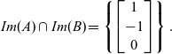 \[Im(A) \cap Im(B) = \left\{ \begin{bmatrix}1 \\-1 \\ 0\end{bmatrix}\right\}.\]
See the theorem:
Theorem 13. (Base for intersection). For all matrices $A_{k \times m}$
and
$A_{k \times m}$
and $B_{k \times n}$
, there is an injective matrix Z such that
$B_{k \times n}$
, there is an injective matrix Z such that
Using the Theorem 12, we obtain the derivation.
Proof
This derivation provides yet another algorithm that returns a basis for the intersection of two subspaces given as input:
Basis for the intersection

From the symmetries property of the graphical syntax (Axiom 2), it is also possible to obtain a program derivation and, consequently, an algorithm for the sum of two subspaces. This is the dual of Theorem 13.
4.3 The exchange lemma
Let V be a finite-dimensional vector space and let $A=(a_1, ..., a_r)$
and
$A=(a_1, ..., a_r)$
and $B=(b_1, ..., b_s)$
be two subspaces of V such that A is linearly independent and
$B=(b_1, ..., b_s)$
be two subspaces of V such that A is linearly independent and
 $$Im{(A)}\subseteq Im{(B)}.$$
The exchange lemma says that $r\leq s$
and that there exists a subspace C formed by the vectors of A and
$r\leq s$
and that there exists a subspace C formed by the vectors of A and $s-r$
vectors of B such that
$s-r$
vectors of B such that $Im{(C)}=Im {(B)}$
. More details can be found in (Barańczuk & Szydło, 2021).
$Im{(C)}=Im {(B)}$
. More details can be found in (Barańczuk & Szydło, 2021).
Example 14. Let $ \left ( e_1,e_2,e_3,e_4 \right )$
be the standard basis in
$ \left ( e_1,e_2,e_3,e_4 \right )$
be the standard basis in $\mathbb{R}^4$
,
$\mathbb{R}^4$
,
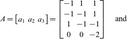 \[A= \begin{bmatrix}a_1 & a_2 & a_3 \\\end{bmatrix}=\begin{bmatrix}-1 & 1 & 1 \\-1 & -1 & 1 \\1 & -1 & -1 \\0 & 0 & -2 \\\end{bmatrix}\quad \text{and}\]
 \[B = \begin{bmatrix}b_1 & b_2 & b_3 & b_4 & b_5\end{bmatrix} = \begin{bmatrix}e_1 & e_2 & e_3 & e_4 & -e_4 \end{bmatrix}.\]
The subspace $C = \begin{bmatrix}a_1 & a_2 & a_3 & b_3 & b_4\end{bmatrix}$
is such that
$C = \begin{bmatrix}a_1 & a_2 & a_3 & b_3 & b_4\end{bmatrix}$
is such that $Im(C)=Im(B)=\mathbb{R}^4$
.
$Im(C)=Im(B)=\mathbb{R}^4$
.
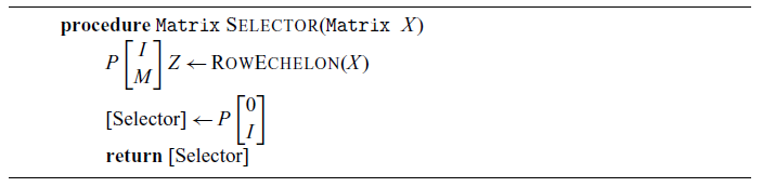
The major issue of the lemma is “selecting” which vectors of B make this true, i.e:
 $$Im{(A)}+Im{(B\;[\text{Selector}])}=Im{(B)}.$$
Inspired by the solution presented by Barańczuk & Szydło (2021), this problem can be stated as the following theorem:
Theorem 14. (Exchange lemma – Verification/Classical version). Let V be a finite-dimensional vector space and let A and B be two subspaces of V such that A is linearly independent and $Im{(A)}\subseteq Im{(B)}$
. Thus, there exists
$Im{(A)}\subseteq Im{(B)}$
. Thus, there exists $X=P\begin{bmatrix}I\\M\end{bmatrix}Z$
, where P is a permutation matrix, I is the identity and Z is invertible, such that
$X=P\begin{bmatrix}I\\M\end{bmatrix}Z$
, where P is a permutation matrix, I is the identity and Z is invertible, such that $A=BX$
and
$A=BX$
and
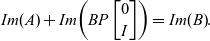 $$Im{(A)}+Im{\left ( B P\begin{bmatrix}0\\I\end{bmatrix} \right )}=Im{(B)}.$$
The expression $P\begin{bmatrix}0\\I\end{bmatrix}$
is the selector that determines the proper vectors of B. The matrix
$P\begin{bmatrix}0\\I\end{bmatrix}$
is the selector that determines the proper vectors of B. The matrix $\begin{bmatrix}0\\I\end{bmatrix}$
has the function of selecting or discarding vectors, while the permutation matrix P determines the order in which this happens. For example, considering B with size
$\begin{bmatrix}0\\I\end{bmatrix}$
has the function of selecting or discarding vectors, while the permutation matrix P determines the order in which this happens. For example, considering B with size $n \times 4$
, a possible selector would be
$n \times 4$
, a possible selector would be
 $$Im\left (\begin{bmatrix}(b_1) & (b_2) & (b_3) & (b_4)\end{bmatrix} \cdot \begin{bmatrix}1 & 0 & 0 & 0\\ 0 & 0 & 0 & 1\\ 0 & 1 & 0 & 0\\ 0 & 0 & 1 & 0\end{bmatrix}\cdot \begin{bmatrix}0 & 0\\ 0 & 0\\ 1 & 0\\ 0 & 1\end{bmatrix} \right ) = Im\left (\begin{bmatrix}(b_4) & (b_2)\end{bmatrix} \right ).$$
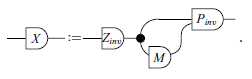
Theorem 14 can be rewritten in graphical syntax as follows:
Theorem 15. (Exchange lemma – Verification/Graphical version). Let A be an injective matrix where
![]() for some matrix B. Then, there exist invertible matrices Z, P and a matrix M such that
for some matrix B. Then, there exist invertible matrices Z, P and a matrix M such that
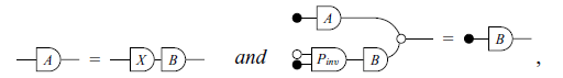
where
Proof
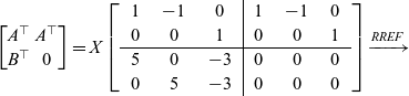
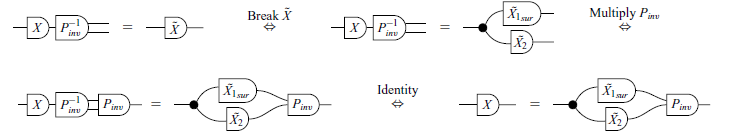
To solve this problem, Barańczuk & Szydło (2021) decomposed the matrix X into row-echelon form. It is possible to do a property derivation to find a way to decompose X by rewriting Theorem 15 as
Theorem 16. (Exchange lemma – Derivation/Graphical version). Let A be an injective matrix and
![]() for some matrix B. Suppose that
for some matrix B. Suppose that
for some matrix X, surjective matrix $\tilde{X}_1$
, matrix
$\tilde{X}_1$
, matrix $\tilde{X}_2$
and invertible matrix P. Then,
$\tilde{X}_2$
and invertible matrix P. Then,
Proof
From
![]() , we can say that
, we can say that $\tilde{X_2}$
is any matrix. On the other hand, the equality
$\tilde{X_2}$
is any matrix. On the other hand, the equality
![]() shows us that
shows us that $\tilde{X_1}$
must be at least surjective. Thus,
$\tilde{X_1}$
must be at least surjective. Thus,
Note that $X=P\begin{bmatrix}\tilde{X_1}\\ \tilde{X_2}\end{bmatrix}$
gives the form of some of the possible solutions to the problem. This derivation also extends the solution initially presented by the reference, but this time is constructed according to the requirements of the problem. We can then write an algorithm that receives the matrix X, uses the derived property, and returns the desired “selector”:
$X=P\begin{bmatrix}\tilde{X_1}\\ \tilde{X_2}\end{bmatrix}$
gives the form of some of the possible solutions to the problem. This derivation also extends the solution initially presented by the reference, but this time is constructed according to the requirements of the problem. We can then write an algorithm that receives the matrix X, uses the derived property, and returns the desired “selector”:
Selector for the Exchange Lemma
5 Conclusions and future work
Throughout this paper, a series of examples involving problems of different nature were presented to demonstrate that graphical linear algebra allows for calculational, point-free reasoning, and program derivation on matrices and linear subspaces.
Future work will mainly focus on graphical syntax. The next step will be to build a characterization for general relationships in graphic notation, expanding their use. Furthermore, a certainly productive direction will be to establish, in diagrams, a schematic description of several other normal forms and matrix factorizations, allowing the exploration and elucidation of the theory of several known theorems and algorithms.
From the development of graphical syntax and its consequent review of concepts, another area to focus on in future work is program derivation. For this, a good start will be to find derivations for theorems previously proven only by verification.
Acknowledgements
Several anonymous individuals are thanked for contributions to these instructions.
Data availability statement
Data availability is not applicable to this article as no new data were created or analysed in this study.
Author contributions
All authors contributed equally to analysing data and reaching conclusions and in writing the paper.
Funding
This study was financed in part by the Coordenação de Aperfeiçoamento de Pessoal de Nível Superior – Brasil (CAPES) – Finance Code 001.
Conflicts of interest
The authors report no conflict of interest.
Appendix A Wikipedia’s Zassenhaus algorithm
Input
Let V be a vector space and U, W two finite-dimensional subspaces of V with the following spanning sets:
 \[U=\left \langle u_{1},\ldots,u_{n} \right \rangle \quad \text{and}\quad W=\left \langle w_{1},...,w_{k} \right \rangle.\]
Finally, let $B_{1},\ldots ,B_{m}$
be linearly independent vectors so that
$B_{1},\ldots ,B_{m}$
be linearly independent vectors so that $u_{i}$
and
$u_{i}$
and $w_{i}$
can be written as
$w_{i}$
can be written as
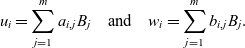 \[u_{i}=\sum_{j=1}^{m}a_{i,j}B_{j} \quad \text{and} \quad w_{i}=\sum_{j=1}^{m}b_{i,j}B_{j}.\]
Output
The algorithm computes the base of the sum $U+W$
and a base of the intersection
$U+W$
and a base of the intersection $U\cap W$
.
$U\cap W$
.
Algorithm
The algorithm creates the following block matrix of size $\left ( \left ( n+k \right )\times\left ( 2m \right ) \right )$
:
$\left ( \left ( n+k \right )\times\left ( 2m \right ) \right )$
:
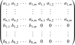 $$\begin{pmatrix} a_{1,1} & a_{1,2} & \cdots & a_{1,m} & a_{1,1} & a_{1,2} & \cdots & a_{1,m}\\ \vdots & \vdots & & \vdots & \vdots & \vdots & & \vdots\\ a_{n,1} & a_{n,2} & \cdots & a_{n,m} & a_{n,1} & a_{n,2} & \cdots & a_{n,m}\\ b_{1,1} & b_{1,2} & \cdots & b_{1,m} & 0 & 0 & \cdots & 0\\ \vdots & \vdots & & \vdots & \vdots & \vdots & & \vdots\\ b_{k,1} & b_{k,2} & \cdots & b_{k,m} & 0 & 0 & \cdots & 0 \end{pmatrix}$$
Using elementary row operations, this matrix is transformed to the row echelon form. Then, it has the following shape:
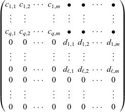 $$\begin{pmatrix} c_{1,1} & c_{1,2} & \cdots & c_{1,m} & \bullet & \bullet & \cdots & \bullet\\ \vdots & \vdots & & \vdots & \vdots & \vdots & & \vdots\\ c_{q,1} & c_{q,2} & \cdots & c_{q,m} & \bullet & \bullet & \cdots & \bullet\\ 0 & 0 & \cdots & 0 & d_{1,1} & d_{1,2} & \cdots & d_{1,m}\\ \vdots & \vdots & & \vdots & \vdots & \vdots & & \vdots\\ 0 & 0 & \cdots & 0 & d_{\ell,1} & d_{\ell,2} & \cdots & d_{\ell,m}\\ 0 & 0 & \cdots & 0 & 0 & 0 & \cdots & 0\\ \vdots & \vdots & & \vdots & \vdots & \vdots & & \vdots\\ 0 & 0 & \cdots & 0 & 0 & 0 & \cdots & 0 \end{pmatrix}$$
Here, $\bullet$
stands for arbitrary numbers, and the vectors
$\bullet$
stands for arbitrary numbers, and the vectors $\left ( c_{p,1},c_{p,2},\ldots,c_{p,m} \right )$
for every
$\left ( c_{p,1},c_{p,2},\ldots,c_{p,m} \right )$
for every $p \in \left \{ 1,...,q \right \}$
and
$p \in \left \{ 1,...,q \right \}$
and $\left ( d_{p,1},d_{p,2},\ldots,d_{p,m} \right )$
for every for every
$\left ( d_{p,1},d_{p,2},\ldots,d_{p,m} \right )$
for every for every $p \in \left \{ 1,...,\ell \right \}$
are nonzero.
$p \in \left \{ 1,...,\ell \right \}$
are nonzero.
Then $(y_{1},\ldots ,y_{q})$
with
$(y_{1},\ldots ,y_{q})$
with
 $$y_{i}:=\sum _{{j=1}}^{m}c_{{i,j}}B_{j}$$
is a basis of $U+W$
and
$U+W$
and $(z_{1},\ldots ,z_{\ell })$
with
$(z_{1},\ldots ,z_{\ell })$
with
 $$z_{i}:=\sum _{{j=1}}^{m}d_{{i,j}}B_{j}$$
is a basis of $U\cap W$
.
$U\cap W$
.
Proof of correctness
First, we define $\pi _{1}:V\times V\to V,(a,b)\mapsto a$
a to be the projection to the first component. Let
$\pi _{1}:V\times V\to V,(a,b)\mapsto a$
a to be the projection to the first component. Let $H:=\{(u,u)\mid u\in U\}+\{(w,0)\mid w\in W\}\subseteq V\times V$
. Then
$H:=\{(u,u)\mid u\in U\}+\{(w,0)\mid w\in W\}\subseteq V\times V$
. Then $\pi _{1}(H)=U+W$
and
$\pi _{1}(H)=U+W$
and $H\cap (0\times V)=0\times (U\cap W)$
. Also,
$H\cap (0\times V)=0\times (U\cap W)$
. Also, $H\cap (0\times V)$
is the kernel of
$H\cap (0\times V)$
is the kernel of ${\pi _{1}|}_{H}$
, the projection restricted to H. Therefore,
${\pi _{1}|}_{H}$
, the projection restricted to H. Therefore, $\dim(H)=\dim(U+W)+\dim(U\cap W)$
. The Zassenhaus algorithm calculates a basis of H. In the first m columns of this matrix, there is a basis
$\dim(H)=\dim(U+W)+\dim(U\cap W)$
. The Zassenhaus algorithm calculates a basis of H. In the first m columns of this matrix, there is a basis $y_{i}$
of
$y_{i}$
of $U+W$
. The rows of the form
$U+W$
. The rows of the form $(0,z_{i})$
(with
$(0,z_{i})$
(with $z_{i}\neq 0$
) are obviously in
$z_{i}\neq 0$
) are obviously in $H\cap (0\times V)$
. Because the matrix is in row echelon form, they are also linearly independent. All rows which are different from zero (
$H\cap (0\times V)$
. Because the matrix is in row echelon form, they are also linearly independent. All rows which are different from zero ( $(y_{i},\bullet )$
and
$(y_{i},\bullet )$
and $(0,z_{i})$
) are a basis of H, so there are
$(0,z_{i})$
) are a basis of H, so there are $\dim(U\cap W)$
such
$\dim(U\cap W)$
such $z_{i}$
s. Therefore, the
$z_{i}$
s. Therefore, the $z_{i}$
s form a basis of
$z_{i}$
s form a basis of $U\cap W$
.
$U\cap W$
.
(Wikipedia contributors, 2023)
Appendix B Zassenhaus: Pointwise proof
Proof [Pointwise notation – Calculational but pointwise]
(1)
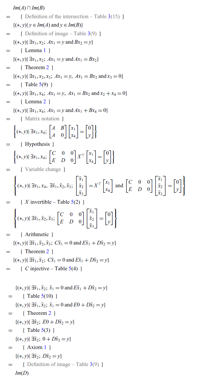
(2)
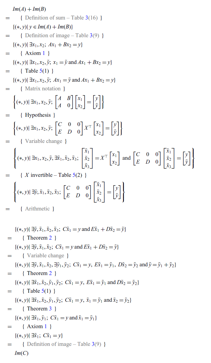


 Open access
Discussions
No Discussions have been published for this article.