


1 Introduction
Invertible computation, also known as reversible computation in physics and more hardware-oriented contexts, is a fundamental concept in computing. It involves computations that run both forward and backward so that the forward/backward semantics form a bijection. (In this paper, we do not concern ourselves with the totality of functions. We call a function a bijection if it is bijective on its actual domain and range, instead of its formal domain and codomain.) Early studies of invertible computation arise from the effort to reduce heat dissipation caused by information-loss in the traditional (unidirectional) computation model (Landauer, Reference Landauer1961). More modern interpretations of the problem include software concerns that are not necessarily connected to the physical realization. Examples of such include developing pairs of programs that are each other’s inverses: serializer and deserializer (Kennedy & Vytiniotis, Reference Kennedy and Vytiniotis2012), parser and printer (Rendel & Ostermann, Reference Rendel and Ostermann2010; Matsuda & Wang, Reference Matsuda and Wang2013, Reference Matsuda and Wang2018b), compressor and decompressor (Srivastava et al., Reference Srivastava, Gulwani, Chaudhuri and Foster2011), and also auxiliary processes in other program transformations such as bidirectionalization (Matsuda et al., Reference Matsuda, Hu, Nakano, Hamana and Takeichi2007).
Invertible (reversible) programming languages are languages that offer primitive support to invertible computations. Examples include Janus (Lutz, Reference Lutz1986; Yokoyama et al.,
2008), Frank’s R (Frank, Reference Frank1997), $\Psi$
-Lisp (Baker, Reference Baker1992), RFun (Yokoyama et al., Reference Yokoyama, Axelsen and Glück2011),
$\Psi$
-Lisp (Baker, Reference Baker1992), RFun (Yokoyama et al., Reference Yokoyama, Axelsen and Glück2011), $\Pi$
/
$\Pi$
/ $\Pi^o$
(James & Sabry, Reference James and Sabry2012), and Inv (Reference Mu, Hu and TakeichiMu et al., 2004b
). The basic idea of these programming languages is to support deterministic forward and backward computation by local inversion: if a forward execution issues (invertible) commands
$\Pi^o$
(James & Sabry, Reference James and Sabry2012), and Inv (Reference Mu, Hu and TakeichiMu et al., 2004b
). The basic idea of these programming languages is to support deterministic forward and backward computation by local inversion: if a forward execution issues (invertible) commands $c_1$
,
$c_1$
, $c_2$
, and
$c_2$
, and $c_3$
in this order, a backward execution issues corresponding inverse commands in the reverse order, as
$c_3$
in this order, a backward execution issues corresponding inverse commands in the reverse order, as $c_3^{-1}$
,
$c_3^{-1}$
, $c_2^{-1}$
, and
$c_2^{-1}$
, and $c_1^{-1}$
. This design has a strong connection to the underlying physical reversibility and is known to be able to achieve reversible Turing completeness (Bennett, Reference Bennett1973); i.e., all computable bijections can be defined.
$c_1^{-1}$
. This design has a strong connection to the underlying physical reversibility and is known to be able to achieve reversible Turing completeness (Bennett, Reference Bennett1973); i.e., all computable bijections can be defined.
However, this requirement of local invertibility does not always match how high-level programs are naturally expressed. As a concrete example, let us see the following toy program that computes the difference of two adjacent elements in a list, where the first element in the input list is kept in the output. For example, we have ${subs} ~ [1,2,5,2,3] = [1,1,3,-3,1]$
.
${subs} ~ [1,2,5,2,3] = [1,1,3,-3,1]$
.
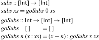
Despite being simple, these kind of transformations are nevertheless useful. For example, a function similar to subs can be found in the preprocessing step of image compression algorithms such as those used for PNG.Footnote 1 Another example is the encoding of bags (multisets) of integers, where subs can be used to convert sorted lists to lists of integers without any constraints (Kennedy & Vytiniotis, Reference Kennedy and Vytiniotis2012).
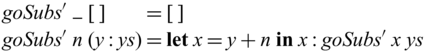
The function subs is invertible. We can define its inverse as below.
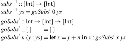
However, subs cannot be expressed directly in existing reversible programming languages. The problem is that, though subs is perfectly invertible, its subcomponent goSubs is not (its first argument is discarded in the empty-list case, and thus the function is not injective). Similar problems are also common in adaptive compression algorithms, where the model (such as a Huffman tree or a dictionary) grows in the same way in both compression and decompression, and the encoding process itself is only invertible after fixing the model at the point.
In the neighboring research area of program inversion, which studies program transformation techniques that derive $f^{-1}$
from f’s defintion, functions like goSubs are identified as partially invertible. Note that this notion of partiality is inspired by partial evaluation, and partial inversion (Romanenko, Reference Romanenko1991; Nishida et al., Reference Nishida, Sakai and Sakabe2005; Almendros-Jiménez & Vidal,
$f^{-1}$
from f’s defintion, functions like goSubs are identified as partially invertible. Note that this notion of partiality is inspired by partial evaluation, and partial inversion (Romanenko, Reference Romanenko1991; Nishida et al., Reference Nishida, Sakai and Sakabe2005; Almendros-Jiménez & Vidal,
2006) allows static (or fixed) parameters whose values are known in inversion and therefore not required to be invertible (for example the first argument of goSubs). (To avoid potential confusion, in this paper, we avoid the use of “partial” when referring to totality, and use the phrase “not-necessarily-total” instead.) However, program inversion by itself does not readily give rise to a design of invertible programming language. Like most program transformations, program inversion may fail, and often for reasons that are not obvious to users. Indeed, the method by Nishida et al. (Reference Nishida, Sakai and Sakabe2005) fails for subs, and for some other methods (Almendros-Jiménez & Vidal, Reference Almendros-Jiménez and Vidal2006; Kirkeby & Glück, Reference Kirkeby and Glück2019, Reference Kirkeby and Glück2020), success depends on the (heuristic) processing order of the expressions.
In this paper, we propose a novel programming language Sparcl
Footnote
2
that for the first time addresses the practical needs of partially invertible programs. The core idea of our proposal is based on a language design that allows invertible and conventional unidirectional computations, which are distinguished by types, to coexist and interact in a single definition. Specifically, inspired by Reference Matsuda and WangMatsuda & Wang (2018c
), our type system contains a special type constructor ![]() (pronounced as “invertible”), where
(pronounced as “invertible”), where ![]() represents A-typed values that are subject to invertible computation. However, having invertible types like
represents A-typed values that are subject to invertible computation. However, having invertible types like ![]() only solves half of the problem. For the applications we consider, exemplified by subs, the unidirectional parts (the first argument of goSubs) may depend on the invertible part (the second argument of goSubs), which complicates the design. (This is the very reason why Nishida et al. (Reference Nishida, Sakai and Sakabe2005)’s partial inversion fails for subs. In other words, a binding-time analysis (Gomard & Jones, Reference Gomard and Jones1991) is not enough (Almendros-Jiménez & Vidal, Reference Almendros-Jiménez and Vidal2006).) This interaction demands conversion from invertible values of type
only solves half of the problem. For the applications we consider, exemplified by subs, the unidirectional parts (the first argument of goSubs) may depend on the invertible part (the second argument of goSubs), which complicates the design. (This is the very reason why Nishida et al. (Reference Nishida, Sakai and Sakabe2005)’s partial inversion fails for subs. In other words, a binding-time analysis (Gomard & Jones, Reference Gomard and Jones1991) is not enough (Almendros-Jiménez & Vidal, Reference Almendros-Jiménez and Vidal2006).) This interaction demands conversion from invertible values of type ![]() to ordinary ones of type A, which only becomes feasible when we leverage the fact that such values can be seen as static (in the sense of partial inversion (Almendros-Jiménez & Vidal, Reference Almendros-Jiménez and Vidal2006)) if the values are already known in both forward and backward directions. The nature of reversibility suggests linearity or relevance (Walker, Reference Walker2004), as discarding of inputs is intrinsically irreversible. In fact, reversible functional programming languages (Baker, Reference Baker1992; Mu et al.,
to ordinary ones of type A, which only becomes feasible when we leverage the fact that such values can be seen as static (in the sense of partial inversion (Almendros-Jiménez & Vidal, Reference Almendros-Jiménez and Vidal2006)) if the values are already known in both forward and backward directions. The nature of reversibility suggests linearity or relevance (Walker, Reference Walker2004), as discarding of inputs is intrinsically irreversible. In fact, reversible functional programming languages (Baker, Reference Baker1992; Mu et al.,
2004b; Yokoyama et al., Reference Yokoyama, Axelsen and Glück2011; James & Sabry, Reference James and Sabry2012; Matsuda &Wang, Reference Matsuda and Wang2013) commonly assume a form of linearity or relevance, and in Sparcl this assumption is made explicit by a linear type system based on $\lambda^q_\to$
(the core system of Linear Haskell (Bernardy et al., Reference Bernardy, Boespflug, Newton, Peyton Jones and Spiwack2018)).
$\lambda^q_\to$
(the core system of Linear Haskell (Bernardy et al., Reference Bernardy, Boespflug, Newton, Peyton Jones and Spiwack2018)).
As a teaser, an invertible version of subs in Sparcl is shown in Figure 1.Footnote
3
In Sparcl, invertible functions from A to B are represented as functions of type ![]() , where
, where $\multimap$
is the constructor for linear functions. Partial invertibility is conveniently expressed by taking additional parameters as in
$\multimap$
is the constructor for linear functions. Partial invertibility is conveniently expressed by taking additional parameters as in ![]() . The
. The ![]() operator converts invertible objects into unidirectional ones. It captures a snapshot of its invertible argument and uses the snapshot as a static value in the body to create a safe local scope for the recursive call. Both the invertible argument and evaluation result of the body are returned as the output to preserve invertibility. The
operator converts invertible objects into unidirectional ones. It captures a snapshot of its invertible argument and uses the snapshot as a static value in the body to create a safe local scope for the recursive call. Both the invertible argument and evaluation result of the body are returned as the output to preserve invertibility. The $\mathrel{{{{{\mathbf{with}}}}}}$
conditions associated with the branches can be seen as postconditions which will be used for invertible case branching. We leave the detailed discussion of the language constructs to later sections, but would like to highlight the fact that looking beyond the surface syntax, the definition is identical in structure to how subs is defined in a conventional language: goSubs has the same recursive pattern with two cases for empty and nonempty lists. This close resemblance to the conventional programming style is what we strive for in the design of Sparcl.
$\mathrel{{{{{\mathbf{with}}}}}}$
conditions associated with the branches can be seen as postconditions which will be used for invertible case branching. We leave the detailed discussion of the language constructs to later sections, but would like to highlight the fact that looking beyond the surface syntax, the definition is identical in structure to how subs is defined in a conventional language: goSubs has the same recursive pattern with two cases for empty and nonempty lists. This close resemblance to the conventional programming style is what we strive for in the design of Sparcl.
Invertible subs in Sparcl.

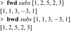
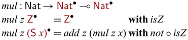
What Sparcl brings to the table is bijectivity guaranteed by construction (potentially with partially invertible functions as auxiliary functions). We can run Sparcl programs in both directions, for example as below, and it is guaranteed that ${{{{\mathbf{fwd}}}}} ~ e ~ v$
results in v’ if and only if
${{{{\mathbf{fwd}}}}} ~ e ~ v$
results in v’ if and only if ${{{{\mathbf{bwd}}}}} ~ e ~ v'$
results in v (
${{{{\mathbf{bwd}}}}} ~ e ~ v'$
results in v ( ${{{{\mathbf{fwd}}}}}$
and
${{{{\mathbf{fwd}}}}}$
and ${{{{\mathbf{bwd}}}}}$
are primitives for forward and backward executions).
${{{{\mathbf{bwd}}}}}$
are primitives for forward and backward executions).
This guarantee of bijectivity is clearly different from the case of (functional) logic programming languages such as Prolog and Curry. Those languages rely on (lazy) generate-and-test (Antoy et al., Reference Antoy, Echahed and Hanus2000) to find inputs corresponding to a given output, a technique that may be adopted in the context of inverse computation (Abramov et al., Reference Abramov, Glück, Klimov, Papers, Virbitskaite and Voronkov2006). However, the generate-and-test strategy has the undesirable consequence of making reversible programming less apparent: it is unclear to programmers whether they are writing bijective programs that may be executed deterministically. Moreover, lazy generation of inputs may cause unpredictable overhead, whereas in reversible languages (Lutz, Reference Lutz1986; Baker,
1992; Frank, Reference Frank1997; Reference Mu, Hu and TakeichiMu et al., 2004b ; Yokoyama et al., Reference Yokoyama, Axelsen and Glück2008, Reference Yokoyama, Axelsen and Glück2011; James & Sabry, Reference James and Sabry2012) including Sparcl, the forward and backward executions of a program take the same steps.
[2]
One might notice from the type of ${{{{\mathbf{pin}}}}}$
that Sparcl is a higher-order language, in the sense that it contains the simply-typed
${{{{\mathbf{pin}}}}}$
that Sparcl is a higher-order language, in the sense that it contains the simply-typed $\lambda$
-calculus (more precisely, the simple multiplicity fragment of
$\lambda$
-calculus (more precisely, the simple multiplicity fragment of $\lambda^q_\to$
(Bernardy et al., Reference Bernardy, Boespflug, Newton, Peyton Jones and Spiwack2018)) as a subsystem. Thus, we can, for example, write an invertible map function in Sparcl as below.
$\lambda^q_\to$
(Bernardy et al., Reference Bernardy, Boespflug, Newton, Peyton Jones and Spiwack2018)) as a subsystem. Thus, we can, for example, write an invertible map function in Sparcl as below.
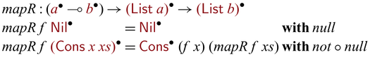
Ideally, we want to program invertible functions by using higher-order functions. But it is not possible. It is known that there is no higher-order invertible languages where $\multimap$
always denotes (not-necessarily-total) bijections. In contrast, there is no issue on having first-order invertible languages as demonstrated by existing reversible languages (see, e.g., RFun (Yokoyama et al., Reference Yokoyama, Axelsen and Glück2011)). Thus, the challenge of designing a higher-order invertible languages lies in finding a sweet spot such that a certain class of functions denote (not-necessarily-total) bijections and programmers can use higher-order functions to abstract computation patterns. Partial invertibility plays an important role here, as functions can be used as static inputs or outputs without violating invertibility. Though this idea has already been considered in the literature (Almendros-Jiménez & Vidal, Reference Almendros-Jiménez and Vidal2006; Mogensen, Reference Mogensen2008; Jacobsen et al., Reference Jacobsen, Kaarsgaard and Thomsen2018) while with restrictions (specifically, no closures), and the advantage is inherited from Reference Matsuda and WangMatsuda &Wang (2018c
) from which Sparcl is inspired, we claim that Sparcl is the first invertible programming language that achieved a proper design for higher-order programming.
$\multimap$
always denotes (not-necessarily-total) bijections. In contrast, there is no issue on having first-order invertible languages as demonstrated by existing reversible languages (see, e.g., RFun (Yokoyama et al., Reference Yokoyama, Axelsen and Glück2011)). Thus, the challenge of designing a higher-order invertible languages lies in finding a sweet spot such that a certain class of functions denote (not-necessarily-total) bijections and programmers can use higher-order functions to abstract computation patterns. Partial invertibility plays an important role here, as functions can be used as static inputs or outputs without violating invertibility. Though this idea has already been considered in the literature (Almendros-Jiménez & Vidal, Reference Almendros-Jiménez and Vidal2006; Mogensen, Reference Mogensen2008; Jacobsen et al., Reference Jacobsen, Kaarsgaard and Thomsen2018) while with restrictions (specifically, no closures), and the advantage is inherited from Reference Matsuda and WangMatsuda &Wang (2018c
) from which Sparcl is inspired, we claim that Sparcl is the first invertible programming language that achieved a proper design for higher-order programming.
In summary, our main contributions are as follows:
• We design Sparcl, a novel higher-order invertible programming language that captures the notion of partial invertibility. It is the first language that handles both clear separation and close integration of unidirectional and invertible computations, enabling new ways of structuring invertible programs. We formally specify the syntax, type system, and semantics of its core system named ${{{{\lambda^{\mathrm{PI}}_{\to}}}}}$
(Section 3).
${{{{\lambda^{\mathrm{PI}}_{\to}}}}}$
(Section 3).
• We state and prove several properties about ${{{{\lambda^{\mathrm{PI}}_{\to}}}}}$
(Section 3.6), including subject reduction, bijectivity, and reversible Turing completeness (Bennett, Reference Bennett1973). We do not state the progress property directly, which is implied by our definitional (Reynolds, Reference Reynolds1998) interpreter written in AgdaFootnote
4
(Section 4).
${{{{\lambda^{\mathrm{PI}}_{\to}}}}}$
(Section 3.6), including subject reduction, bijectivity, and reversible Turing completeness (Bennett, Reference Bennett1973). We do not state the progress property directly, which is implied by our definitional (Reynolds, Reference Reynolds1998) interpreter written in AgdaFootnote
4
(Section 4).
• We demonstrate the utility of Sparcl with nontrivial examples: tree rebuilding from inorder and preoder traversals (Mu & Bird, Reference Mu and Bird2003) and simplified versions of compression algorithms including Huffman coding, arithmetic coding, and LZ77 (Ziv & Lempel, Reference Ziv and Lempel1977) (Section 5).
In addition, a prototype implementation of Sparcl is available from https://github.com/kztk-m/sparcl,which also contains more examples. All the artifacts are linked from the Sparcl web page (https://bx-lang.github.io/EXHIBIT/sparcl.html).Footnote 5
A preliminary version of this paper appeared in ICFP20 (Matsuda & Wang, Reference Matsuda and Wang2020) with the same title. The major changes include a description of our Agda implementation in Section 4 and the arithmetic coding and LZ77 examples in Sections 5.3 and 5.4. Moreover, the related work section (Section 6) is updated to include work published after the preliminary version (Matsuda & Wang, Reference Matsuda and Wang2020).
2 Overview
In this section, we informally introduce the essential constructs of Sparcl and demonstrate their use with small examples.
2.1 Linear-typed programming
Linearity (or weaker relevance) is commonly adopted in reversible functional languages (Baker, Reference Baker1992; Reference Mu, Hu and TakeichiMu et al., 2004b
; Yokoyama et al., Reference Yokoyama, Axelsen and Glück2011; James & Sabry, Reference James and Sabry2012; Matsuda & Wang, Reference Matsuda and Wang2013) to exclude noninjective functions such as constant functions. Sparcl is no exception (we will revisit its importance in Section 2.3) and adopts a linear type system based on $\lambda^q_{\to}$
(the core system of Linear Haskell (Bernardy et al., Reference Bernardy, Boespflug, Newton, Peyton Jones and Spiwack2018)). A feature of the type system is its function type
$\lambda^q_{\to}$
(the core system of Linear Haskell (Bernardy et al., Reference Bernardy, Boespflug, Newton, Peyton Jones and Spiwack2018)). A feature of the type system is its function type $A \to_{p} B$
, where the arrow is annotated by the argument’s multiplicity (1 or
$A \to_{p} B$
, where the arrow is annotated by the argument’s multiplicity (1 or $\omega$
). Here,
$\omega$
). Here, $A \to_{1} B$
denotes linear functions that use the input exactly once, while
$A \to_{1} B$
denotes linear functions that use the input exactly once, while $A \to_{\omega} B$
denotes unrestricted functions that have no restriction on the use of its input. The following are some examples of linear and unrestricted functions.
$A \to_{\omega} B$
denotes unrestricted functions that have no restriction on the use of its input. The following are some examples of linear and unrestricted functions.
Observe that the double used x twice and const discards y; hence, the corresponding arrows must be annotated by $\omega$
. The purpose of the type system is to ensure bijectivity. But having linearity alone is not sufficient. We will come back to this point after showing invertible programming in Sparcl. Readers who are familiar with linear-type systems that have the exponential operator
$\omega$
. The purpose of the type system is to ensure bijectivity. But having linearity alone is not sufficient. We will come back to this point after showing invertible programming in Sparcl. Readers who are familiar with linear-type systems that have the exponential operator $!$
(Wadler, Reference Wadler1993) may view
$!$
(Wadler, Reference Wadler1993) may view $A \to_{\omega} B$
as
$A \to_{\omega} B$
as $!A \multimap B$
. A small deviation from the (simply-typed fragment of)
$!A \multimap B$
. A small deviation from the (simply-typed fragment of) $\lambda^q_{\to}$
is that Sparcl is equipped with rank-1 polymorphism with qualified typing (Jones, Reference Jones1995) and type inference (Matsuda, Reference Matsuda2020). For example, the system infers the following types for the following functions.
$\lambda^q_{\to}$
is that Sparcl is equipped with rank-1 polymorphism with qualified typing (Jones, Reference Jones1995) and type inference (Matsuda, Reference Matsuda2020). For example, the system infers the following types for the following functions.

In first two examples, p is arbitrary (i.e., 1 or $\omega$
); in the last example, the predicate
$\omega$
); in the last example, the predicate $p \le q$
states an ordering of multiplicity, where
$p \le q$
states an ordering of multiplicity, where $1 \le \omega$
.Footnote
6
This predicate states that if an argument is linear then it cannot be passed to an unrestricted function, as an unrestricted function may use its argument arbitrary many times. A more in-depth discussion of the surface type system is beyond the scope of this paper, but note that unlike the implementation of Linear Haskell as of GHC 9.0.XFootnote
7
which checks linearity only when type signatures are given explicitly, Sparcl can infer linear types thanks to the use of qualified typing.
$1 \le \omega$
.Footnote
6
This predicate states that if an argument is linear then it cannot be passed to an unrestricted function, as an unrestricted function may use its argument arbitrary many times. A more in-depth discussion of the surface type system is beyond the scope of this paper, but note that unlike the implementation of Linear Haskell as of GHC 9.0.XFootnote
7
which checks linearity only when type signatures are given explicitly, Sparcl can infer linear types thanks to the use of qualified typing.
For simplicity, we sometimes write $\multimap$
for
$\multimap$
for $\to_{1}$
and simply
$\to_{1}$
and simply $\to$
for
$\to$
for $\to_{\omega}$
when showing programming examples in Sparcl.
$\to_{\omega}$
when showing programming examples in Sparcl.
2.2 Multiplication
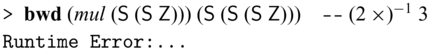
One of the simplest examples of partially invertible programs is multiplication (Nishida et al., 2005). Suppose that we have a datatype of natural numbers defined as below.
In Sparcl, constructors have linear types: ![]() .
.
We define multiplication in term of addition, which is also partially invertible.Footnote 8
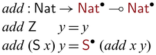
As mentioned in the introduction, we use the type constructor ![]() to distinguish data that are subject to invertible computation (such as
to distinguish data that are subject to invertible computation (such as ![]() ) and those that are not (such as
) and those that are not (such as ![]() ): when the latter is fixed, a partially invertible function is turned into a (not-necessarily-total) bijection, for example,
): when the latter is fixed, a partially invertible function is turned into a (not-necessarily-total) bijection, for example, ![]() . (For those who read the paper with colors, the arguments of
. (For those who read the paper with colors, the arguments of ![]() are highlighted in
are highlighted in ![]() .) Values of
.) Values of ![]() -types are constructed by lifted constructors such as
-types are constructed by lifted constructors such as ![]() . In the forward direction,
. In the forward direction, ![]() to the input, and in the backward direction, it strips one
to the input, and in the backward direction, it strips one $\mathsf{S}$
(and the evaluation gets stuck if
$\mathsf{S}$
(and the evaluation gets stuck if $\mathsf{Z}$
is found). In general, since constructors by nature are always bijective (though not necessarily total in the backward direction), every constructor
$\mathsf{Z}$
is found). In general, since constructors by nature are always bijective (though not necessarily total in the backward direction), every constructor $\mathsf{C} : \sigma_1 \multimap \dots \multimap \sigma_n \multimap \tau$
automatically give rise to a corresponding lifted version
$\mathsf{C} : \sigma_1 \multimap \dots \multimap \sigma_n \multimap \tau$
automatically give rise to a corresponding lifted version ![]() .
.
A partially invertible multiplication function can be defined by using add as below.Footnote 9
An interesting feature in the mul program is the invertible pattern matching (Yokoyama
et al., 2008) indicated by patterns ![]() (here, we annotate patterns instead of constructors). Invertible pattern matching is a branching mechanism that executes bidirectionally: the forward direction basically performs the standard pattern matching, the backward direction employs an additional
(here, we annotate patterns instead of constructors). Invertible pattern matching is a branching mechanism that executes bidirectionally: the forward direction basically performs the standard pattern matching, the backward direction employs an additional $\mathrel{{{{{\mathbf{with}}}}}}$
clause to determine the branch to be taken. For example,
$\mathrel{{{{{\mathbf{with}}}}}}$
clause to determine the branch to be taken. For example, ![]() , in the forward direction, values are matched against the forms
, in the forward direction, values are matched against the forms $\mathsf{Z}$
and
$\mathsf{Z}$
and $\mathsf{S} ~ x$
; in the backward direction, the
$\mathsf{S} ~ x$
; in the backward direction, the $\mathrel{{{{{\mathbf{with}}}}}}$
conditions are checked upon an output of the function
$\mathrel{{{{{\mathbf{with}}}}}}$
conditions are checked upon an output of the function ${mul} ~ n$
: if
${mul} ~ n$
: if ${isZ}: {\mathsf{Nat}} \to \mathsf{Bool}$
returns
${isZ}: {\mathsf{Nat}} \to \mathsf{Bool}$
returns $\mathsf{True}$
, the first branch is chosen, otherwise the second branch is chosen. When the second branch is taken, the backward computation of
$\mathsf{True}$
, the first branch is chosen, otherwise the second branch is chosen. When the second branch is taken, the backward computation of ${add} ~ n$
is performed, which essentially subtracts n, followed by recursively applying the backward computation of
${add} ~ n$
is performed, which essentially subtracts n, followed by recursively applying the backward computation of ${mul} ~ {n}$
to the result. As the last step, the final result is enclosed with
${mul} ~ {n}$
to the result. As the last step, the final result is enclosed with $\mathsf{S}$
and returned. In other words, the backward behavior of
$\mathsf{S}$
and returned. In other words, the backward behavior of ${mul} ~ n$
recursively tries to subtract n and returns the count of successful subtractions.
${mul} ~ n$
recursively tries to subtract n and returns the count of successful subtractions.
In Sparcl, $\mathrel{{{{{\mathbf{with}}}}}}$
conditions are provided by programmers and expected to be exclusive; the conditions are enforced at run-time: the
$\mathrel{{{{{\mathbf{with}}}}}}$
conditions are provided by programmers and expected to be exclusive; the conditions are enforced at run-time: the $\mathrel{{{{{\mathbf{with}}}}}}$
conditions are asserted to be postconditions on the branches’ values. Specifically, the branch’s
$\mathrel{{{{{\mathbf{with}}}}}}$
conditions are asserted to be postconditions on the branches’ values. Specifically, the branch’s $\mathrel{{{{{\mathbf{with}}}}}}$
condition is a positive assertion while all the other branches’ ones are negative assertions. Thus, the forward computation fails when the branch’s
$\mathrel{{{{{\mathbf{with}}}}}}$
condition is a positive assertion while all the other branches’ ones are negative assertions. Thus, the forward computation fails when the branch’s $\mathrel{{{{{\mathbf{with}}}}}}$
condition is not satisfied, or any of the other
$\mathrel{{{{{\mathbf{with}}}}}}$
condition is not satisfied, or any of the other $\mathrel{{{{{\mathbf{with}}}}}}$
conditions is also satisfied. This exclusiveness enables the backward computation to uniquely identify the branch (Lutz, Reference Lutz1986; Yokoyama et al., Reference Yokoyama, Axelsen and Glück2008). Sometimes we may omit the
$\mathrel{{{{{\mathbf{with}}}}}}$
conditions is also satisfied. This exclusiveness enables the backward computation to uniquely identify the branch (Lutz, Reference Lutz1986; Yokoyama et al., Reference Yokoyama, Axelsen and Glück2008). Sometimes we may omit the $\mathrel{{{{{\mathbf{with}}}}}}$
condition of the last branch, as it can be inferred as the negation of the conjunction of all the others. For example, in the definition of goSubs the second branch’s
$\mathrel{{{{{\mathbf{with}}}}}}$
condition of the last branch, as it can be inferred as the negation of the conjunction of all the others. For example, in the definition of goSubs the second branch’s $\mathrel{{{{{\mathbf{with}}}}}}$
condition is
$\mathrel{{{{{\mathbf{with}}}}}}$
condition is ![]() . One could use sophisticated types such as refinement types to infer
. One could use sophisticated types such as refinement types to infer $\mathrel{{{{{\mathbf{with}}}}}}$
-conditions and even statically enforce exclusiveness instead of assertion checking. However, we stick to simple types in this paper as our primal goal is to establish the basic design of Sparcl.
$\mathrel{{{{{\mathbf{with}}}}}}$
-conditions and even statically enforce exclusiveness instead of assertion checking. However, we stick to simple types in this paper as our primal goal is to establish the basic design of Sparcl.
An astute reader may wonder what bijection ${mul} ~ \mathsf{Z}$
defines, as zero times n is zero for any n. In fact, it defines a non-total bijection that in the forward direction the domain of the function contains only
${mul} ~ \mathsf{Z}$
defines, as zero times n is zero for any n. In fact, it defines a non-total bijection that in the forward direction the domain of the function contains only $\mathsf{Z}$
, i.e., the trivial bijection between
$\mathsf{Z}$
, i.e., the trivial bijection between ${\mathsf{Z}}$
and
${\mathsf{Z}}$
and ${\mathsf{Z}}$
.
${\mathsf{Z}}$
.
2.3 Why linearity itself is insufficient but still matters
The primal role of linearity is to prohibit values from being discarded or copied, and Sparcl is no exception. However, linearity itself is insufficient for partially invertible programming.
To start with, it is clear that $\multimap$
is not equivalent to not-necessarily-total bijections. For example, the function
$\multimap$
is not equivalent to not-necessarily-total bijections. For example, the function $\lambda x.x ~ (\lambda y.y) ~ (\lambda z.z) : ((\sigma \multimap \sigma) \multimap (\sigma \multimap \sigma)\multimap (\sigma \multimap \sigma)) \multimap \sigma \multimap \sigma$
returns
$\lambda x.x ~ (\lambda y.y) ~ (\lambda z.z) : ((\sigma \multimap \sigma) \multimap (\sigma \multimap \sigma)\multimap (\sigma \multimap \sigma)) \multimap \sigma \multimap \sigma$
returns $\lambda y.y$
for both
$\lambda y.y$
for both $\lambda f.\lambda g.\lambda x.f ~ (g ~ x)$
and
$\lambda f.\lambda g.\lambda x.f ~ (g ~ x)$
and $\lambda f.\lambda g.\lambda x.g ~ (f ~ x)$
. Theoretically, this comes from the fact that the category of (not-necessarily-total) bijections is not (monoidal) closed. Thus, as discussed above, the challenge is to find a sweet spot where a certain class of functions denote (not-necessarily-total) bijections.
$\lambda f.\lambda g.\lambda x.g ~ (f ~ x)$
. Theoretically, this comes from the fact that the category of (not-necessarily-total) bijections is not (monoidal) closed. Thus, as discussed above, the challenge is to find a sweet spot where a certain class of functions denote (not-necessarily-total) bijections.
It is known that a linear calculus concerning tensor products ( $\otimes$
) and linear functions
$\otimes$
) and linear functions $(\multimap)$
(even with exponentials (
$(\multimap)$
(even with exponentials ( $!$
)) can be modeled in the Int-construction (Joyal et al., Reference Joyal, Street and Verity1996) of the category of not-necessarily-total bijections (Abramsky et al., Reference Abramsky, Haghverdi and Scott2002; Abramsky, Reference Abramsky2005. Here, roughly speaking, first-order functions on base types can be understood as not-necessarily-total bijections. However, it is also known that such a system cannot be easily extended to include sum-types nor invertible pattern matching (Abramsky, Reference Abramsky2005, Section 7).
$!$
)) can be modeled in the Int-construction (Joyal et al., Reference Joyal, Street and Verity1996) of the category of not-necessarily-total bijections (Abramsky et al., Reference Abramsky, Haghverdi and Scott2002; Abramsky, Reference Abramsky2005. Here, roughly speaking, first-order functions on base types can be understood as not-necessarily-total bijections. However, it is also known that such a system cannot be easily extended to include sum-types nor invertible pattern matching (Abramsky, Reference Abramsky2005, Section 7).
Moreover, linearity does not express partiality as in partially invertible computations. For example, without the ![]() types, function add can have type
types, function add can have type $\mathsf{Nat} \multimap \mathsf{Nat} \multimap \mathsf{Nat}$
(note the linear use of the first argument), which does not specify which parameter is a fixed one. It even has type
$\mathsf{Nat} \multimap \mathsf{Nat} \multimap \mathsf{Nat}$
(note the linear use of the first argument), which does not specify which parameter is a fixed one. It even has type $\mathsf{Nat} \otimes \mathsf{Nat} \multimap \mathsf{Nat}$
after uncurrying though addition is clearly not fully invertible. These are the reasons why we separate the invertible world and the unidirectional world by using
$\mathsf{Nat} \otimes \mathsf{Nat} \multimap \mathsf{Nat}$
after uncurrying though addition is clearly not fully invertible. These are the reasons why we separate the invertible world and the unidirectional world by using ![]() , inspired by staged languages (Nielson & Nielson, Reference Nielson and Nielson1992; Moggi, Reference Moggi1998; Davies & Pfenning, Reference Davies and Pfenning2001). Readers familiar with staged languages may see
, inspired by staged languages (Nielson & Nielson, Reference Nielson and Nielson1992; Moggi, Reference Moggi1998; Davies & Pfenning, Reference Davies and Pfenning2001). Readers familiar with staged languages may see ![]() as residual code of type A, which will be executed forward or backward at the second stage to output or input A-typed values.
as residual code of type A, which will be executed forward or backward at the second stage to output or input A-typed values.
On the other hand, ![]() does not replace the need for linearity either. Without linearity,
does not replace the need for linearity either. Without linearity, ![]() -typed values may be discarded or duplicated, which may lead to non-bijectivity. Unlike discarding, the exclusion of duplication is debatable as the inverse of duplication can be given as equality check (Glück and Kawabe, Reference Glück and Kawabe2003). So it is our design choice to exclude duplication (contraction) in addition to discarding (weakening) to avoid unpredictable failures that may be caused by the equality checks. Without contraction, users are still able to implement duplication for datatypes with decidable equality (see Section 5.1.3). However, this design requires duplication (and the potential of failing) to be made explicit, which improves the predictability of the system. Having explicit duplication is not uncommon in this context (Reference Mu, Hu and TakeichiMu et al., 2004b
; Yokoyama et al., Reference Yokoyama, Axelsen and Glück2011).
-typed values may be discarded or duplicated, which may lead to non-bijectivity. Unlike discarding, the exclusion of duplication is debatable as the inverse of duplication can be given as equality check (Glück and Kawabe, Reference Glück and Kawabe2003). So it is our design choice to exclude duplication (contraction) in addition to discarding (weakening) to avoid unpredictable failures that may be caused by the equality checks. Without contraction, users are still able to implement duplication for datatypes with decidable equality (see Section 5.1.3). However, this design requires duplication (and the potential of failing) to be made explicit, which improves the predictability of the system. Having explicit duplication is not uncommon in this context (Reference Mu, Hu and TakeichiMu et al., 2004b
; Yokoyama et al., Reference Yokoyama, Axelsen and Glück2011).
Another design choice we made is to admit types like ![]() to simplify the formalization; otherwise, kinds will be needed to distinguish types that can be used in
to simplify the formalization; otherwise, kinds will be needed to distinguish types that can be used in ![]() from general types, and subkinding to allow running and importing bijections (Sections 2.4 and 2.5). Such types are not very useful though, as function- or invertible-typed values cannot be inspected during invertible computations.
from general types, and subkinding to allow running and importing bijections (Sections 2.4 and 2.5). Such types are not very useful though, as function- or invertible-typed values cannot be inspected during invertible computations.
2.4 Running reversible computation
Sparcl provides primitive functions to execute invertible functions in either directions: ![]() . For example, we have:
. For example, we have:
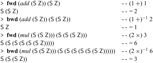
Of course, the forward and backward computations may not be total. For example, the following expression (legitimately) fails.
The guarantee Sparcl offers is that derived bijections are total with respect to the functions’ actual domains and ranges; i.e., ${{{{\mathbf{fwd}}}}} ~ e ~ v$
results in u, then
${{{{\mathbf{fwd}}}}} ~ e ~ v$
results in u, then ${{{{\mathbf{bwd}}}}} ~ e ~ u$
results in v, and vice versa (Section 3.6.2).
${{{{\mathbf{bwd}}}}} ~ e ~ u$
results in v, and vice versa (Section 3.6.2).
Linearity plays a role here. Linear calculi are considered resource-aware in the sense that linear variables will be lost once used. In our case, resources are ![]() -typed values, as
-typed values, as ![]() represents (a part of) an input or (a part of) an output of a bijection being constructed, which must be retained throughout the computation. This is why the first argument of
represents (a part of) an input or (a part of) an output of a bijection being constructed, which must be retained throughout the computation. This is why the first argument of ${{{{\mathbf{fwd}}}}}$
/
${{{{\mathbf{fwd}}}}}$
/ ${{{{\mathbf{bwd}}}}}$
is unrestricted rather than linear. Very roughly speaking, an expression that can be passed to an unrestricted function cannot contain linear variables, or “resources”. Thus, a function of type
${{{{\mathbf{bwd}}}}}$
is unrestricted rather than linear. Very roughly speaking, an expression that can be passed to an unrestricted function cannot contain linear variables, or “resources”. Thus, a function of type ![]() passed to
passed to ${{{{\mathbf{fwd}}}}}$
/
${{{{\mathbf{fwd}}}}}$
/ ${{{{\mathbf{bwd}}}}}$
cannot use any resources other than one value of type
${{{{\mathbf{bwd}}}}}$
cannot use any resources other than one value of type ![]() to produce one value of type
to produce one value of type ![]() . In other words, all and only information from
. In other words, all and only information from ![]() is retained in
is retained in ![]() , guaranteeing bijectivity. As a result, Sparcl’s type system effectively rejects code like
, guaranteeing bijectivity. As a result, Sparcl’s type system effectively rejects code like ![]() as x’s multiplicity is
as x’s multiplicity is $\omega$
in both cases. In the former case, x is discarded and multiplicity in our system is either 1 or
$\omega$
in both cases. In the former case, x is discarded and multiplicity in our system is either 1 or $\omega$
. In the latter case, x appears in the first argument of
$\omega$
. In the latter case, x appears in the first argument of ${{{{\mathbf{fwd}}}}}$
, which is unrestricted.
${{{{\mathbf{fwd}}}}}$
, which is unrestricted.
2.5 Importing existing invertible functions
Bijectivity is not uncommon in computer science or mathematics, and there already exist many established algorithms that are bijective. Examples include nontrivial results in number theory or category theory, and manipulation of primitive or sophisticated data structures such as Burrows-Wheeler transformations on suffix arrays.
Instead of (re)writing them in Sparcl, the language provides a mechanism to directly import existing bijections (as a pair of functions) to construct valid Sparcl programs: ![]() converts a pair of functions into a function on
converts a pair of functions into a function on ![]() -typed values, expecting that the pair of functions form mutual inverses. For example, by
-typed values, expecting that the pair of functions form mutual inverses. For example, by ${{{{\mathbf{lift}}}}}$
, we can define addInt as below
${{{{\mathbf{lift}}}}}$
, we can define addInt as below
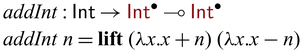
The use of ${{{{\mathbf{lift}}}}}$
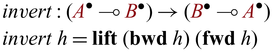
allows one to create primitive bijections to be composed by the various constructs in Sparcl. Another interesting use of
${{{{\mathbf{lift}}}}}$
allows one to create primitive bijections to be composed by the various constructs in Sparcl. Another interesting use of ${{{{\mathbf{lift}}}}}$
is to implement in-language inversion.
${{{{\mathbf{lift}}}}}$
is to implement in-language inversion.
2.6 Composing partially invertible functions
Partially invertible functions in Sparcl expect arguments of both ![]() and
and ![]() types, which sometimes makes the calling of such functions interesting. This phenomenon is particularly noticeable in recursive calls where values of type
types, which sometimes makes the calling of such functions interesting. This phenomenon is particularly noticeable in recursive calls where values of type ![]() may need to be fed into function calls expecting values of type A. In this case, it becomes necessary to convert
may need to be fed into function calls expecting values of type A. In this case, it becomes necessary to convert ![]() -typed values to A-typed one. To avoid the risk of violating invertibility, such conversions are carefully managed in Sparcl through a special function
-typed values to A-typed one. To avoid the risk of violating invertibility, such conversions are carefully managed in Sparcl through a special function ![]()
![]() , inspired by the depGame function in Kennedy & Vytiniotis (Reference Kennedy and Vytiniotis2012) and reversible updates (Axelsen et al., Reference Axelsen, Glück and Yokoyama2007) in reversible imperative languages (Lutz, Reference Lutz1986; Frank, Reference Frank1997; Yokoyama et al., Reference Yokoyama, Axelsen and Glück2008; Glück & Yokoyama, Reference Glück and Yokoyama2016). The function
, inspired by the depGame function in Kennedy & Vytiniotis (Reference Kennedy and Vytiniotis2012) and reversible updates (Axelsen et al., Reference Axelsen, Glück and Yokoyama2007) in reversible imperative languages (Lutz, Reference Lutz1986; Frank, Reference Frank1997; Yokoyama et al., Reference Yokoyama, Axelsen and Glück2008; Glück & Yokoyama, Reference Glück and Yokoyama2016). The function ${{{{\mathbf{pin}}}}}$
creates a static snapshot of its first argument (
${{{{\mathbf{pin}}}}}$
creates a static snapshot of its first argument (![]() ) and uses the snapshot (A) in its second argument. Bijectivity of a function involving
) and uses the snapshot (A) in its second argument. Bijectivity of a function involving ${{{{\mathbf{pin}}}}}$
is guaranteed as the original
${{{{\mathbf{pin}}}}}$
is guaranteed as the original ![]() value is retained in the output
value is retained in the output ![]() together with the evaluation result of the second argument (
together with the evaluation result of the second argument (![]() ). For example,
). For example, ![]() , which defines the mapping between (n,m) and
, which defines the mapping between (n,m) and $(n,n+m)$
, is bijective. We will define the function
$(n,n+m)$
, is bijective. We will define the function ${{{{\mathbf{pin}}}}}$
and formally state the correctness property in Section 3.
${{{{\mathbf{pin}}}}}$
and formally state the correctness property in Section 3.
Let us revisit the example in Section 1. The partially invertible version of goSubs can be implemented via ${{{{\mathbf{pin}}}}}$
as below.
${{{{\mathbf{pin}}}}}$
as below.
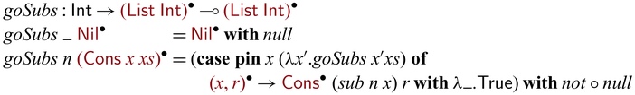
Here, we used ${{{{\mathbf{pin}}}}}$
to convert
${{{{\mathbf{pin}}}}}$
to convert ![]() to
to $x':{\mathsf{Int}}$
in order to pass it to the recursive call of goSubs. In the backward direction,
$x':{\mathsf{Int}}$
in order to pass it to the recursive call of goSubs. In the backward direction, ${goSubs} ~ n$
executes as follows.Footnote
10
${goSubs} ~ n$
executes as follows.Footnote
10
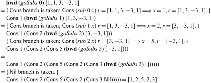
Note that the first arguments of (recursive) calls of goSubs (which are static) have the same values (1, 2, 5, 2, and 3) in both forward/backward executions, distinguishing their uses from those of the invertible arguments. As one can see, ${goSubs} ~ {n}$
behaves exactly like the hand-written goSubs’ in
${goSubs} ~ {n}$
behaves exactly like the hand-written goSubs’ in ${subs}^{-1}$
which is reproduced below.
${subs}^{-1}$
which is reproduced below.
The use of ${{{{\mathbf{pin}}}}}$
commonly results in an invertible
${{{{\mathbf{pin}}}}}$
commonly results in an invertible ${{{{\mathbf{case}}}}}$
with a single branch, as we see in goSubs above. We capture this pattern with an invertible
${{{{\mathbf{case}}}}}$
with a single branch, as we see in goSubs above. We capture this pattern with an invertible ${{{{\mathbf{let}}}}}$
as a shorthand notation, which enables us to write
${{{{\mathbf{let}}}}}$
as a shorthand notation, which enables us to write ![]() . The definition of goSubs shown in Section 1 uses this shorthand notation, which is reproduced in Figure 2(a).
. The definition of goSubs shown in Section 1 uses this shorthand notation, which is reproduced in Figure 2(a).
Side-by-side comparison of partially invertible (a) and fully invertible (b) versions of subs.

We would like to emphasize that partial invertibility, as supported in Sparcl, is key to concise function definitions. In Figure 2, we show side-by-side two versions of the same program written in the same language: the one on the left allows partial invertibility whereas the one on the right requires all functions (include the intermediate ones) to be fully invertible (note the different types in the two versions of goSubs and sub). As a result, goSubsF is much harder to define and the code becomes fragile and error-prone. This advantage of Sparcl, which is already evident in this small example, becomes decisive when dealing with larger programs, especially those requiring complex manipulation of static values (for example, the Huffman coding in Section 5.2).
We end this section with a theoretical remark. One might wonder why ![]() is not a monad. This intuitively comes from the fact that the first and second stages are in different languages (the standard one and an invertible one, respectively) with different semantics. More formally,
is not a monad. This intuitively comes from the fact that the first and second stages are in different languages (the standard one and an invertible one, respectively) with different semantics. More formally, ![]() , which brings a type in the second stage into the first stage, forms a functor, but the functor is not endo. Recall that
, which brings a type in the second stage into the first stage, forms a functor, but the functor is not endo. Recall that ![]() represents residual code in an invertible system of type A; that is,
represents residual code in an invertible system of type A; that is, ![]() and its component A belong to different categories (though we have not formally described them).Footnote
11
One then might wonder whether
and its component A belong to different categories (though we have not formally described them).Footnote
11
One then might wonder whether ![]() is a relative monad (Altenkirch et al., Reference Altenkirch, Chapman and Uustalu2010). To form a relative monad, one needs to find a functor that has the same domain and codomain as (the functor corresponding to)
is a relative monad (Altenkirch et al., Reference Altenkirch, Chapman and Uustalu2010). To form a relative monad, one needs to find a functor that has the same domain and codomain as (the functor corresponding to) ![]() . It is unclear whether there exists such a functor other than
. It is unclear whether there exists such a functor other than ![]() itself; in this case, the relative monad operations do not provide any additional expressive power.
itself; in this case, the relative monad operations do not provide any additional expressive power.
2.7 Implementations
We have implemented a proof-of-concept interpreter for Sparcl including the linear type system, which is available from https://github.com/kztk-m/sparcl. The implementation adds two small but useful extensions to what is presented in this paper. First, the implementation allows nonlinear constructors, such as $\mathsf{MkUn} : a \to \mathsf{Un} ~ a$
which serves as
$\mathsf{MkUn} : a \to \mathsf{Un} ~ a$
which serves as $!$
and helps us to write a function that returns both linear and unrestricted results. Misusing such constructors in invertible pattern matching is guarded against by the type system (otherwise it may lead to discarding or copying of invertible values). Second, the implementation uses the first-match principle for both forward and backward computations. That is, both patterns and
$!$
and helps us to write a function that returns both linear and unrestricted results. Misusing such constructors in invertible pattern matching is guarded against by the type system (otherwise it may lead to discarding or copying of invertible values). Second, the implementation uses the first-match principle for both forward and backward computations. That is, both patterns and $\mathrel{{{{{\mathbf{with}}}}}}$
conditions are examined from top to bottom. Recall also that the implementation uses a non-indentation-sensitive syntax for simplicity as mentioned in Section 1.
$\mathrel{{{{{\mathbf{with}}}}}}$
conditions are examined from top to bottom. Recall also that the implementation uses a non-indentation-sensitive syntax for simplicity as mentioned in Section 1.
It is worth noting that the implementation uses Matsuda (Reference Matsuda2020)’s type inference to infer linear types effectively without requiring any annotations. Hence, the type annotations in this paper are more for documentation purposes.
As part of our effort to prove type safety (subject reduction and progress), we also produced a parallel implementation in Agda to serve as proofs (Section 3.6), available from https://github.com/kztk-m/sparcl-agda.
3 Core system: ${{{{\lambda^{\mathrm{PI}}_{\to}}}}}$

This section introduces ${{{{\lambda^{\mathrm{PI}}_{\to}}}}}$
, the core system that Sparcl is built on. Our design mixes ideas of linear-typed programming and meta-programming. As mentioned in Section 2.1, the language is based on (the simple multiplicity fragment of)
${{{{\lambda^{\mathrm{PI}}_{\to}}}}}$
, the core system that Sparcl is built on. Our design mixes ideas of linear-typed programming and meta-programming. As mentioned in Section 2.1, the language is based on (the simple multiplicity fragment of) $\lambda^q_{\to}$
(Bernardy et al., Reference Bernardy, Boespflug, Newton, Peyton Jones and Spiwack2018), and, as mentioned in Section 2.3, it is also two-staged (Nielson & Nielson, Reference Nielson and Nielson1992; Moggi, Reference Moggi1998) with different meta and object languages. Specifically, the meta stage is a usual call-by-value language (i.e., unidirectional), and the object stage is an invertible language. By having the two stages, partial invertibility is made explicit in this formalization.
$\lambda^q_{\to}$
(Bernardy et al., Reference Bernardy, Boespflug, Newton, Peyton Jones and Spiwack2018), and, as mentioned in Section 2.3, it is also two-staged (Nielson & Nielson, Reference Nielson and Nielson1992; Moggi, Reference Moggi1998) with different meta and object languages. Specifically, the meta stage is a usual call-by-value language (i.e., unidirectional), and the object stage is an invertible language. By having the two stages, partial invertibility is made explicit in this formalization.
In what follows, we use a number of notational conventions. A vector notation ![]() denotes a sequence such as
denotes a sequence such as $t_1,\dots,t_n$
or
$t_1,\dots,t_n$
or $t_1; \dots ; t_n$
, where each
$t_1; \dots ; t_n$
, where each $t_i$
can be of any syntactic category and the delimiter (such as “,” and “;”) can differ depending on the context; we also refer to the length of the sequence by
$t_i$
can be of any syntactic category and the delimiter (such as “,” and “;”) can differ depending on the context; we also refer to the length of the sequence by ![]() . In addition, we may refer to an element in the sequence
. In addition, we may refer to an element in the sequence ![]() as
as $t_i$
. A simultaneous substitution of
$t_i$
. A simultaneous substitution of $x_1,\dots,x_n$
in t with
$x_1,\dots,x_n$
in t with $s_1,\dots,s_n$
is denoted as
$s_1,\dots,s_n$
is denoted as $t[s_1/x_1,\dots,s_n/x_n]$
, which may also be written as
$t[s_1/x_1,\dots,s_n/x_n]$
, which may also be written as ![]() .
.
3.1 Central concept: Bijections at the heart
The surface language of Sparcl is designed for programming partially invertible functions, which are turned into bijections (by fixing the static arguments) for execution. This fact is highlighted in the core system ${{{{\lambda^{\mathrm{PI}}_{\to}}}}}$
where we have a primitive bijection type
${{{{\lambda^{\mathrm{PI}}_{\to}}}}}$
where we have a primitive bijection type ${A \rightleftharpoons B}$
, which is inhabited by bijections constructed from functions of type
${A \rightleftharpoons B}$
, which is inhabited by bijections constructed from functions of type ![]() . Technically, having a dedicated bijection type facilitates reasoning. For example, we may now straightforwardly state that “values of a bijection type
. Technically, having a dedicated bijection type facilitates reasoning. For example, we may now straightforwardly state that “values of a bijection type ${A \rightleftharpoons B}$
are bijections between A and B” (Corollary 3.4).
${A \rightleftharpoons B}$
are bijections between A and B” (Corollary 3.4).
Accordingly, the ${{{{\mathbf{fwd}}}}}$
and
${{{{\mathbf{fwd}}}}}$
and ${{{{\mathbf{bwd}}}}}$
functions for execution in Sparcl are divided into application operators
${{{{\mathbf{bwd}}}}}$
functions for execution in Sparcl are divided into application operators $ \triangleright $
and
$ \triangleright $
and $ \triangleleft $
that apply bijection-typed values and an
$ \triangleleft $
that apply bijection-typed values and an ${{{{\mathbf{unlift}}}}}$
operator for constructing bijections from functions of type
${{{{\mathbf{unlift}}}}}$
operator for constructing bijections from functions of type ![]() . For example, we have
. For example, we have ${{{{\mathbf{unlift}}}}} ~ ({add} ~ \mathsf{(S Z))} : {\mathsf{Nat} \rightleftharpoons \mathsf{Nat}}$
(where
${{{{\mathbf{unlift}}}}} ~ ({add} ~ \mathsf{(S Z))} : {\mathsf{Nat} \rightleftharpoons \mathsf{Nat}}$
(where ![]() is defined in Section 2), and the bijection can be executed as
is defined in Section 2), and the bijection can be executed as $ {{{{\mathbf{unlift}}}}} ~ ({add} ~ \mathsf{(S Z))} \triangleright \mathsf{S Z} $
resulting in
$ {{{{\mathbf{unlift}}}}} ~ ({add} ~ \mathsf{(S Z))} \triangleright \mathsf{S Z} $
resulting in $\mathsf{S (S Z)}$
and
$\mathsf{S (S Z)}$
and $ {{{{\mathbf{unlift}}}}} ~ ({add} ~ \mathsf{(S Z))} \triangleleft \mathsf{S (S Z)} $
resulting in
$ {{{{\mathbf{unlift}}}}} ~ ({add} ~ \mathsf{(S Z))} \triangleleft \mathsf{S (S Z)} $
resulting in $S Z$
. In fact, the operators
$S Z$
. In fact, the operators ${{{{\mathbf{fwd}}}}}$
and
${{{{\mathbf{fwd}}}}}$
and ${{{{\mathbf{bwd}}}}}$
are now derived in
${{{{\mathbf{bwd}}}}}$
are now derived in ${{{{\lambda^{\mathrm{PI}}_{\to}}}}}$
, as
${{{{\lambda^{\mathrm{PI}}_{\to}}}}}$
, as ${{{{\mathbf{fwd}}}}} = \lambda_\omega h. \lambda_\omega x. {{{{\mathbf{unlift}}}}} ~ h \triangleright x$
and
${{{{\mathbf{fwd}}}}} = \lambda_\omega h. \lambda_\omega x. {{{{\mathbf{unlift}}}}} ~ h \triangleright x$
and ${{{{\mathbf{bwd}}}}} = \lambda_\omega h. \lambda_\omega x. {{{{\mathbf{unlift}}}}} ~ h \triangleleft x$
.
${{{{\mathbf{bwd}}}}} = \lambda_\omega h. \lambda_\omega x. {{{{\mathbf{unlift}}}}} ~ h \triangleleft x$
.
[2] Here, $\omega$
of
$\omega$
of $\lambda_\omega$
indicates that the bound variable can be used arbitrary many. In contrast,
$\lambda_\omega$
indicates that the bound variable can be used arbitrary many. In contrast, $\lambda_1$
indicates that the bound variable must be used linearly. Hence, for example,
$\lambda_1$
indicates that the bound variable must be used linearly. Hence, for example, $\lambda_1 x.\mathsf{Z}$
and
$\lambda_1 x.\mathsf{Z}$
and $\lambda_1 x.(x,x)$
are ill-typed, while
$\lambda_1 x.(x,x)$
are ill-typed, while $\lambda_1 x.x$
,
$\lambda_1 x.x$
, $\lambda_\omega x.\mathsf{Z}$
and
$\lambda_\omega x.\mathsf{Z}$
and $\lambda_\omega x. (x,x)$
are well-typed. Similarly, we also annotate (unidirectional)
$\lambda_\omega x. (x,x)$
are well-typed. Similarly, we also annotate (unidirectional) ${{{{\mathbf{case}}}}}$
s with the multiplicity of the variables bound by pattern matching. Thus, for example,
${{{{\mathbf{case}}}}}$
s with the multiplicity of the variables bound by pattern matching. Thus, for example, ${{{{\mathbf{case}}}}}_1~\mathsf{S} ~ \mathsf{Z}~{{{{\mathbf{of}}}}}~\{ \mathsf{S} ~ x \to (x,x) \}$
and
${{{{\mathbf{case}}}}}_1~\mathsf{S} ~ \mathsf{Z}~{{{{\mathbf{of}}}}}~\{ \mathsf{S} ~ x \to (x,x) \}$
and $\lambda_1 x. {{{{\mathbf{case}}}}}_\omega~x~{{{{\mathbf{of}}}}} \{ \mathsf{S} ~ y \to \mathsf{Z} \}$
are ill-typed.
$\lambda_1 x. {{{{\mathbf{case}}}}}_\omega~x~{{{{\mathbf{of}}}}} \{ \mathsf{S} ~ y \to \mathsf{Z} \}$
are ill-typed.
3.2 Syntax
The syntax of ${{{{\lambda^{\mathrm{PI}}_{\to}}}}}$
is given as below.
${{{{\lambda^{\mathrm{PI}}_{\to}}}}}$
is given as below.
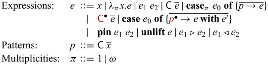
There are three lines for the various constructs of expressions. The ones in the first line are standard except the annotations in $\lambda$
and
$\lambda$
and ${{{{\mathbf{case}}}}}$
that determine the multiplicity of the variables introduced by the binders:
${{{{\mathbf{case}}}}}$
that determine the multiplicity of the variables introduced by the binders: $\pi = 1$
means that the bound variable is linear, and
$\pi = 1$
means that the bound variable is linear, and $\pi = \omega$
means there is no restriction. These annotations are omitted in the surface language as they are inferred. The second and third lines consist of constructs that deal with invertibility. As mentioned above,
$\pi = \omega$
means there is no restriction. These annotations are omitted in the surface language as they are inferred. The second and third lines consist of constructs that deal with invertibility. As mentioned above, ${{{{\mathbf{unlift}}}}} ~ e$
,
${{{{\mathbf{unlift}}}}} ~ e$
, $e_1 \triangleright e_2$
, and
$e_1 \triangleright e_2$
, and $e_1 \triangleleft e_2$
handles bijections which can be used to encode
$e_1 \triangleleft e_2$
handles bijections which can be used to encode ${{{{\mathbf{fwd}}}}}$
and
${{{{\mathbf{fwd}}}}}$
and ${{{{\mathbf{bwd}}}}}$
in Sparcl. We have already seen lifted constructors, invertible
${{{{\mathbf{bwd}}}}}$
in Sparcl. We have already seen lifted constructors, invertible ${{{{\mathbf{case}}}}}$
, and
${{{{\mathbf{case}}}}}$
, and ${{{{\mathbf{pin}}}}}$
in Section 2. For simplicity, we assume that
${{{{\mathbf{pin}}}}}$
in Section 2. For simplicity, we assume that ${{{{\mathbf{pin}}}}}$
,
${{{{\mathbf{pin}}}}}$
, $\mathsf{C}$
and
$\mathsf{C}$
and ![]() are fully applied. Lifted constructor expressions
are fully applied. Lifted constructor expressions ![]() and invertible
and invertible ${{{{\mathbf{case}}}}}$
s are basic invertible primitives in
${{{{\mathbf{case}}}}}$
s are basic invertible primitives in ${{{{\lambda^{\mathrm{PI}}_{\to}}}}}$
. They are enough to make our system reversible Turing complete Bennett (Reference Bennett1973) (Theorem 3.5); i.e., all bijections can be implemented in the language. For simplicity, we assume that patterns are nonoverlapping both for unidirectional and invertible
${{{{\lambda^{\mathrm{PI}}_{\to}}}}}$
. They are enough to make our system reversible Turing complete Bennett (Reference Bennett1973) (Theorem 3.5); i.e., all bijections can be implemented in the language. For simplicity, we assume that patterns are nonoverlapping both for unidirectional and invertible ${{{{\mathbf{case}}}}}$
s. We do not include
${{{{\mathbf{case}}}}}$
s. We do not include ${{{{\mathbf{lift}}}}}$
, which imports external code into Sparcl, as it is by definition unsafe. Instead, we will discuss it separately in Section 3.7.
${{{{\mathbf{lift}}}}}$
, which imports external code into Sparcl, as it is by definition unsafe. Instead, we will discuss it separately in Section 3.7.
Different from conventional reversible/invertible programming languages, the constructs ${{{{\mathbf{unlift}}}}}$
(together with
${{{{\mathbf{unlift}}}}}$
(together with $ \triangleright $
and
$ \triangleright $
and $ \triangleleft $
) and
$ \triangleleft $
) and ${{{{\mathbf{pin}}}}}$
support communication between the unidirectional world and the invertible world. The
${{{{\mathbf{pin}}}}}$
support communication between the unidirectional world and the invertible world. The ${{{{\mathbf{unlift}}}}}$
construct together with
${{{{\mathbf{unlift}}}}}$
construct together with $ \triangleright $
and
$ \triangleright $
and $ \triangleleft $
runs invertible computation in the unidirectional world. The
$ \triangleleft $
runs invertible computation in the unidirectional world. The ${{{{\mathbf{pin}}}}}$
operator is the key to partiality; it enables us to temporarily convert a value in the invertible world into a value in the unidirectional world.
${{{{\mathbf{pin}}}}}$
operator is the key to partiality; it enables us to temporarily convert a value in the invertible world into a value in the unidirectional world.
3.3 Types
Types in ${{{{\lambda^{\mathrm{PI}}_{\to}}}}}$
are defined as below.
${{{{\lambda^{\mathrm{PI}}_{\to}}}}}$
are defined as below.
Here, $\alpha$
denotes a type variable,
$\alpha$
denotes a type variable, $\mathsf{T}$
denotes a type constructor,
$\mathsf{T}$
denotes a type constructor, $A \to_\pi B$
is a function type annotated with the argument’s multiplicity
$A \to_\pi B$
is a function type annotated with the argument’s multiplicity $\pi$
,
$\pi$
, ![]() marks invertibility, and
marks invertibility, and ${A \rightleftharpoons B}$
is a bijection type.
${A \rightleftharpoons B}$
is a bijection type.
Each type constructor $\mathsf{T}$
comes with a set of constructors
$\mathsf{T}$
comes with a set of constructors $\mathsf{C}$
of type
$\mathsf{C}$
of type
with ![]() for any i.Footnote
12
Type variables
for any i.Footnote
12
Type variables $\alpha$
are only used for types of constructors in the language. For example, the standard multiplicative product
$\alpha$
are only used for types of constructors in the language. For example, the standard multiplicative product $\otimes$
and additive sum
$\otimes$
and additive sum $\oplus$
Wadler (Reference Wadler1993) are represented by the following constructors.
$\oplus$
Wadler (Reference Wadler1993) are represented by the following constructors.
We assume that the set of type constructors at least include $\otimes$
and
$\otimes$
and $\mathsf{Bool}$
, where
$\mathsf{Bool}$
, where $\mathsf{Bool}$
has the constructors
$\mathsf{Bool}$
has the constructors $\mathsf{True} : \mathsf{Bool}$
and
$\mathsf{True} : \mathsf{Bool}$
and $\mathsf{False} : \mathsf{Bool}$
. Types can be recursive via constructors; for example, we can have a list type
$\mathsf{False} : \mathsf{Bool}$
. Types can be recursive via constructors; for example, we can have a list type $\mathsf{List} ~ \alpha$
with the following constructors.
$\mathsf{List} ~ \alpha$
with the following constructors.
We may write ![]() for
for $A_1 \multimap A_2 \multimap \cdots \multimap A_n \multimap B$
(when n is zero,
$A_1 \multimap A_2 \multimap \cdots \multimap A_n \multimap B$
(when n is zero, ![]() is B). We shall also instantiate constructors implicitly and write
is B). We shall also instantiate constructors implicitly and write ![]() when there is a constructor
when there is a constructor ![]() for each i. Thus, we assume all types in our discussions are closed.
for each i. Thus, we assume all types in our discussions are closed.
Negative recursive types are allowed in our system, which, for example, enables us to define general recursions without primitive fixpoint operators. Specifically, via $\mathsf{F}$
with the constructor
$\mathsf{F}$
with the constructor $ \mathsf{MkF} : (\mathsf{F} ~ \alpha \to \alpha) \multimap \mathsf{F} ~ \alpha$
, we have a fixpoint operator as below.
$ \mathsf{MkF} : (\mathsf{F} ~ \alpha \to \alpha) \multimap \mathsf{F} ~ \alpha$
, we have a fixpoint operator as below.

Here, out has type $\mathsf{F} ~ C \multimap \mathsf{F} ~ C \to C$
for any C (in this case
$\mathsf{F} ~ C \multimap \mathsf{F} ~ C \to C$
for any C (in this case $C = A \to_{\pi} B$
), and thus
$C = A \to_{\pi} B$
), and thus ${fix}_\pi$
has type
${fix}_\pi$
has type $((A \to_\pi B) \to (A \to_\pi B)) \to A \to_\pi B$
.
$((A \to_\pi B) \to (A \to_\pi B)) \to A \to_\pi B$
.
The most special type in the language is ![]() , which is the invertible version of A. More specifically, the invertible type
, which is the invertible version of A. More specifically, the invertible type ![]() represents residual code in an invertible system that are executed forward and backward at the second stage to output and input A-typed values. Values of type
represents residual code in an invertible system that are executed forward and backward at the second stage to output and input A-typed values. Values of type ![]() must be treated linearly and can only be manipulated by invertible operations, such as lifted constructors, invertible pattern matching, and
must be treated linearly and can only be manipulated by invertible operations, such as lifted constructors, invertible pattern matching, and ${{{{\mathbf{pin}}}}}$
. To keep our type system simple, or more specifically single-kinded, we allow types like
${{{{\mathbf{pin}}}}}$
. To keep our type system simple, or more specifically single-kinded, we allow types like ![]() , while the category of (not-necessarily-total) bijections are not closed and
, while the category of (not-necessarily-total) bijections are not closed and ${{{{\lambda^{\mathrm{PI}}_{\to}}}}}$
has no third stage. These types do not pose any problem, as such components cannot be inspected in invertible computation by any means (except in
${{{{\lambda^{\mathrm{PI}}_{\to}}}}}$
has no third stage. These types do not pose any problem, as such components cannot be inspected in invertible computation by any means (except in $\mathrel{{{{{\mathbf{with}}}}}}$
conditions, which are unidirectional, i.e., run at the first stage).
$\mathrel{{{{{\mathbf{with}}}}}}$
conditions, which are unidirectional, i.e., run at the first stage).
Note that we consider the primitive bijection types ${A \rightleftharpoons B}$
as separate from
${A \rightleftharpoons B}$
as separate from $(A \to B) \otimes (B \to A)$
. This separation is purely for reasoning; in our theoretical development, we will show that
$(A \to B) \otimes (B \to A)$
. This separation is purely for reasoning; in our theoretical development, we will show that ${A \rightleftharpoons B}$
denotes pairs of functions that are guaranteed to form (not-necessarily-total) bijections (corollary:correctness).
${A \rightleftharpoons B}$
denotes pairs of functions that are guaranteed to form (not-necessarily-total) bijections (corollary:correctness).
3.4 Typing relation
A typing environment is a mapping from variables x to pairs of type A and its multiplicity $\pi$
, meaning that x has type A and can be used
$\pi$
, meaning that x has type A and can be used $\pi$
-many times. We write
$\pi$
-many times. We write $x_1:_{\pi_1} A_1, \dots, x_n:_{\pi_n} B_n$
instead of
$x_1:_{\pi_1} A_1, \dots, x_n:_{\pi_n} B_n$
instead of $\{ x_1 \mapsto (A_1 , \pi_1), \dots, x_n \mapsto (B_n, \pi_n) \}$
for readability and write
$\{ x_1 \mapsto (A_1 , \pi_1), \dots, x_n \mapsto (B_n, \pi_n) \}$
for readability and write ${epsilon}$
for the empty environment. Reflecting the two stages, we adopt a dual context system (Davies & Pfenning, Reference Davies and Pfenning2001), which has unidirectional and invertible environments, denoted by
${epsilon}$
for the empty environment. Reflecting the two stages, we adopt a dual context system (Davies & Pfenning, Reference Davies and Pfenning2001), which has unidirectional and invertible environments, denoted by $\Gamma$
and
$\Gamma$
and $\Theta$
respectively. This separation of the two is purely theoretical, for the purpose of facilitating reasoning when we interpret
$\Theta$
respectively. This separation of the two is purely theoretical, for the purpose of facilitating reasoning when we interpret ![]() -typed expressions that are closed in unidirectional variables but may have free variables in
-typed expressions that are closed in unidirectional variables but may have free variables in $\Theta$
as bijections. In fact, our prototype implementation does not distinguish the two environments. For all invertible environments
$\Theta$
as bijections. In fact, our prototype implementation does not distinguish the two environments. For all invertible environments $\Theta$
, without the loss of generality we assume that the associated multiplicities must be 1, i.e.,
$\Theta$
, without the loss of generality we assume that the associated multiplicities must be 1, i.e., $\Theta(x) = (A_x, 1)$
for any
$\Theta(x) = (A_x, 1)$
for any $x \in \mathsf{dom}(\Theta)$
. Thus, we shall sometimes omit multiplicities for
$x \in \mathsf{dom}(\Theta)$
. Thus, we shall sometimes omit multiplicities for $\Theta$
. This assumption is actually an invariant in our system since any variables introduced in
$\Theta$
. This assumption is actually an invariant in our system since any variables introduced in $\Theta$
must have multiplicity 1. We make this explicit in order to simplify the theoretical discussions. Moreover, we assume that the domains of
$\Theta$
must have multiplicity 1. We make this explicit in order to simplify the theoretical discussions. Moreover, we assume that the domains of $\Gamma$
and
$\Gamma$
and $\Theta$
are disjoint.
$\Theta$
are disjoint.
Given two unidirectional typing environments $\Gamma_1$
and
$\Gamma_1$
and $\Gamma_2$
, we define the addition
$\Gamma_2$
, we define the addition $\Gamma_1 + \Gamma_2$
as below.
$\Gamma_1 + \Gamma_2$
as below.

If $\mathsf{dom}(\Gamma_1)$
and
$\mathsf{dom}(\Gamma_1)$
and $\mathsf{dom}(\Gamma_2)$
are disjoint, we sometimes write
$\mathsf{dom}(\Gamma_2)$
are disjoint, we sometimes write $\Gamma_1, \Gamma_2$
instead of
$\Gamma_1, \Gamma_2$
instead of $\Gamma_1 + \Gamma_2$
to emphasize the disjointness. A similar addition applies to invertible environments. But as only multiplicity 1 is allowed in
$\Gamma_1 + \Gamma_2$
to emphasize the disjointness. A similar addition applies to invertible environments. But as only multiplicity 1 is allowed in $\Theta$
,
$\Theta$
, $\Theta_1 + \Theta_2 = \Theta$
implicitly implies
$\Theta_1 + \Theta_2 = \Theta$
implicitly implies $\mathsf{dom}(\Theta_1) \cap \mathsf{dom}(\Theta_2) = \emptyset$
.
$\mathsf{dom}(\Theta_1) \cap \mathsf{dom}(\Theta_2) = \emptyset$
.
We define multiplication of multiplicities as below.
Given $\Gamma = x_1 :_{\pi_1} A_1, \dots, x_n :_{\pi_n} A_n$
, we write
$\Gamma = x_1 :_{\pi_1} A_1, \dots, x_n :_{\pi_n} A_n$
, we write $\pi \Gamma$
for the environment
$\pi \Gamma$
for the environment $x_1 :_{\pi \pi_1} A_1, \dots, x_n :_{\pi\pi_n} A_n$
. A similar notation applies to invertible environments. Again,
$x_1 :_{\pi \pi_1} A_1, \dots, x_n :_{\pi\pi_n} A_n$
. A similar notation applies to invertible environments. Again, $\omega \Theta' = \Theta$
means that
$\omega \Theta' = \Theta$
means that $\Theta' = {epsilon}$
. Notice that it can hold that
$\Theta' = {epsilon}$
. Notice that it can hold that $\Gamma = \Gamma + \Gamma$
and
$\Gamma = \Gamma + \Gamma$
and $\Gamma = \omega \Gamma = 1 \Gamma$
if
$\Gamma = \omega \Gamma = 1 \Gamma$
if $\Gamma(x) = (_,\omega)$
for all
$\Gamma(x) = (_,\omega)$
for all $x \in \mathsf{dom}(\Gamma)$
.
$x \in \mathsf{dom}(\Gamma)$
.
The typing relation $\Gamma; \Theta \vdash e : A$
reads that under environments
$\Gamma; \Theta \vdash e : A$
reads that under environments $\Gamma$
and
$\Gamma$
and $\Theta$
, expression e has type A (Figure 3). The definition basically follows
$\Theta$
, expression e has type A (Figure 3). The definition basically follows $\lambda^q_\to$
(Bernardy et al., Reference Bernardy, Boespflug, Newton, Peyton Jones and Spiwack2018) except having two environments for the two stages. Although multiplicities in
$\lambda^q_\to$
(Bernardy et al., Reference Bernardy, Boespflug, Newton, Peyton Jones and Spiwack2018) except having two environments for the two stages. Although multiplicities in $\Theta$
are always 1, some of the typing rules refers to
$\Theta$
are always 1, some of the typing rules refers to $\omega \Theta$
(which implies
$\omega \Theta$
(which implies $\Theta = {epsilon}$
) in the conclusion parts, to emphasize that
$\Theta = {epsilon}$
) in the conclusion parts, to emphasize that $\Gamma$
and
$\Gamma$
and $\Theta$
are treated similarly by the rules. The idea underlying this type system is that, together with the operational semantics in Section 3.5, a term-in-context
$\Theta$
are treated similarly by the rules. The idea underlying this type system is that, together with the operational semantics in Section 3.5, a term-in-context ![]() defines a piece of code representing a bijection between
defines a piece of code representing a bijection between $\Theta$
and A, and hence
$\Theta$
and A, and hence ${epsilon}; {epsilon} \vdash e' : {A \rightleftharpoons B}$
defines a bijection between A and B (see Section 3.6). Our Agda implementation explained in Section 4, which we mentioned in Sections 1 and 2.7, follows this idea with some generalization. The typing rules in Figure 3 are divided into three groups: the standard ones inherited from
${epsilon}; {epsilon} \vdash e' : {A \rightleftharpoons B}$
defines a bijection between A and B (see Section 3.6). Our Agda implementation explained in Section 4, which we mentioned in Sections 1 and 2.7, follows this idea with some generalization. The typing rules in Figure 3 are divided into three groups: the standard ones inherited from $\lambda^q_\to$
(T-Var, T-Abs, T-App, T-Con, and T-Case), the ones for the invertible part (T-RVar, T-RCon, and T-RCase), and the ones for the interaction between the two (T-Pin, T-Unlift, T-FApp, and T-BApp).
$\lambda^q_\to$
(T-Var, T-Abs, T-App, T-Con, and T-Case), the ones for the invertible part (T-RVar, T-RCon, and T-RCase), and the ones for the interaction between the two (T-Pin, T-Unlift, T-FApp, and T-BApp).
Typing rules for expressions and patterns.
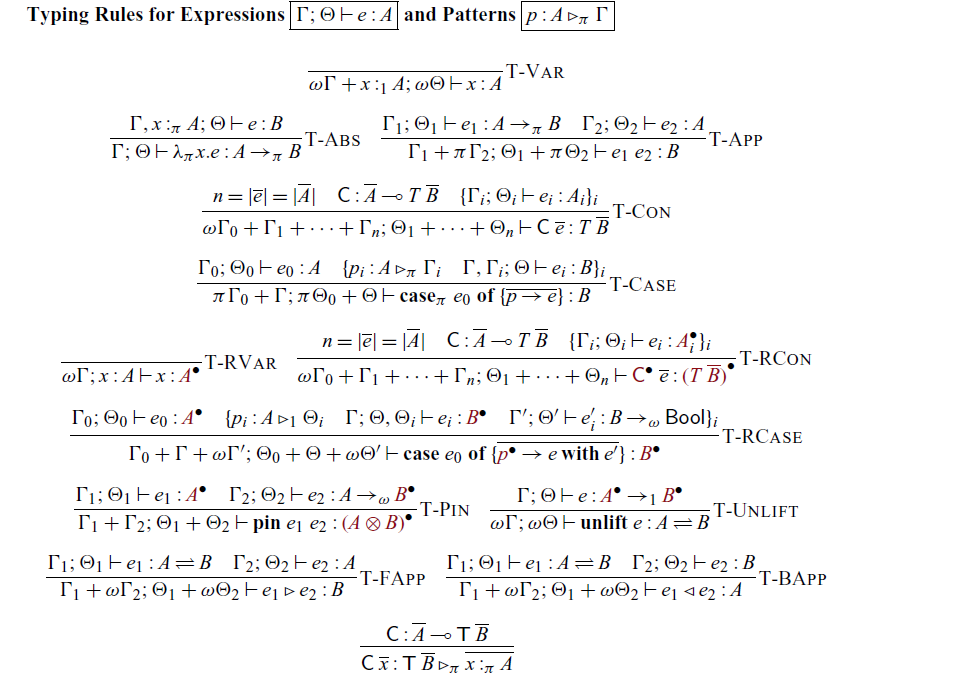
Intuitively, the multiplicity of a variable represents the usage of a resource to be associated with the variable. Hence, multiplicities in $\Gamma$
and
$\Gamma$
and $\Theta$
are synthesized rather than checked in typing. This viewpoint is useful for understanding T-App and T-Case; it is natural that, if an expression e is used
$\Theta$
are synthesized rather than checked in typing. This viewpoint is useful for understanding T-App and T-Case; it is natural that, if an expression e is used $\pi$
times, the multiplicities of variables in e are multiplied by
$\pi$
times, the multiplicities of variables in e are multiplied by $\pi$
. Discarding variables, or weakening, is performed in the rules T-Var, T-RVar, T-Con, and T-RCon which can be leaves in a derivation tree. Note that weakening is not allowed for
$\pi$
. Discarding variables, or weakening, is performed in the rules T-Var, T-RVar, T-Con, and T-RCon which can be leaves in a derivation tree. Note that weakening is not allowed for $\Theta$
-variables as they are linear.
$\Theta$
-variables as they are linear.
The typing rules for the invertible part would need additional explanation. In T-RVar, x has type ![]() if the invertible typing environment is the singleton mapping
if the invertible typing environment is the singleton mapping $x : A$
. One explanation for this is that
$x : A$
. One explanation for this is that $\Theta$
represents the typing environment for the object (i.e., invertible) system. Another explanation is that we simply omit
$\Theta$
represents the typing environment for the object (i.e., invertible) system. Another explanation is that we simply omit ![]() as all variables in
as all variables in $\Theta$
must have types of the form
$\Theta$
must have types of the form ![]() . Rule T-RCon says that we can lift a constructor to the invertible world leveraging the injective nature of the constructor. Rule T-RCase says that the invertible
. Rule T-RCon says that we can lift a constructor to the invertible world leveraging the injective nature of the constructor. Rule T-RCase says that the invertible ${{{{\mathbf{case}}}}}$
is for pattern-matching on
${{{{\mathbf{case}}}}}$
is for pattern-matching on ![]() -typed data; the pattern matching is done in the invertible world, and thus the bodies of the branches must also have
-typed data; the pattern matching is done in the invertible world, and thus the bodies of the branches must also have ![]() -types. Recall that the
-types. Recall that the $\mathrel{{{{{\mathbf{with}}}}}}$
-conditions (
$\mathrel{{{{{\mathbf{with}}}}}}$
-conditions ( $e'_i$
) are used for deciding which branch is used in backward computation. The type
$e'_i$
) are used for deciding which branch is used in backward computation. The type $B \to_\omega \mathsf{Bool}$
indicates that they are conventional unrestricted functions, and
$B \to_\omega \mathsf{Bool}$
indicates that they are conventional unrestricted functions, and $\omega \Gamma'$
and
$\omega \Gamma'$
and $\omega \Theta'$
in the conclusion part of the rule indicates that their uses are unconstrained. Notice that, since the linearity comes only from the use of
$\omega \Theta'$
in the conclusion part of the rule indicates that their uses are unconstrained. Notice that, since the linearity comes only from the use of ![]() -typed values, there is little motivation to use linear variables to define conventional functions in
-typed values, there is little motivation to use linear variables to define conventional functions in ${{{{\lambda^{\mathrm{PI}}_{\to}}}}}$
. The operators
${{{{\lambda^{\mathrm{PI}}_{\to}}}}}$
. The operators ${{{{\mathbf{pin}}}}}$
,
${{{{\mathbf{pin}}}}}$
, ${{{{\mathbf{unlift}}}}}$
,
${{{{\mathbf{unlift}}}}}$
, $ \triangleright $
, and
$ \triangleright $
, and $ \triangleleft $
are special in
$ \triangleleft $
are special in ${{{{\lambda^{\mathrm{PI}}_{\to}}}}}$
. The operator
${{{{\lambda^{\mathrm{PI}}_{\to}}}}}$
. The operator ${{{{\mathbf{pin}}}}}$
is simply a fully applied version of the one in Section 2; so we do not repeat the explanation. Rules T-Unlift, T-FApp, and T-BApp are inherited from the types of
${{{{\mathbf{pin}}}}}$
is simply a fully applied version of the one in Section 2; so we do not repeat the explanation. Rules T-Unlift, T-FApp, and T-BApp are inherited from the types of ${{{{\mathbf{fwd}}}}}$
and
${{{{\mathbf{fwd}}}}}$
and ${{{{\mathbf{bwd}}}}}$
in Section 2. Recall that
${{{{\mathbf{bwd}}}}}$
in Section 2. Recall that $\omega \Theta$
ensures
$\omega \Theta$
ensures $\Theta = {epsilon}$
, and thus the arguments of
$\Theta = {epsilon}$
, and thus the arguments of ${{{{\mathbf{unlift}}}}}$
and constructed bijections must be closed in terms of invertible variables. It might look a little weird that
${{{{\mathbf{unlift}}}}}$
and constructed bijections must be closed in terms of invertible variables. It might look a little weird that $e_1 \triangleright e_2$
/
$e_1 \triangleright e_2$
/ $e_1 \triangleleft e_2$
uses
$e_1 \triangleleft e_2$
uses $e_1$
linearly; this is not a problem because
$e_1$
linearly; this is not a problem because $\Theta_1$
in T-FApp/T-BApp must be empty for expressions that occur in evaluation (Lemma 3.2).
$\Theta_1$
in T-FApp/T-BApp must be empty for expressions that occur in evaluation (Lemma 3.2).
3.5 Operational semantics
The semantics of ${{{{\lambda^{\mathrm{PI}}_{\to}}}}}$
consists of three evaluation relations: unidirectional, forward, and backward. The unidirectional evaluation evaluates away the unidirectional constructs such as
${{{{\lambda^{\mathrm{PI}}_{\to}}}}}$
consists of three evaluation relations: unidirectional, forward, and backward. The unidirectional evaluation evaluates away the unidirectional constructs such as $\lambda$
-abstractions and applications, and the forward and backward evaluation specifies bijections.
$\lambda$
-abstractions and applications, and the forward and backward evaluation specifies bijections.
For example, let us consider an expression ![]() . Due to
. Due to $\lambda$
-abstractions and function applications, it is not immediately clear how we can interpret the expression as a bijection. The unidirectional evaluation
$\lambda$
-abstractions and function applications, it is not immediately clear how we can interpret the expression as a bijection. The unidirectional evaluation ![]() is used to evaluate these unidirectional constructs away to make way for the forward and backward evaluation to interpret the residual term. For the above expression, we have
is used to evaluate these unidirectional constructs away to make way for the forward and backward evaluation to interpret the residual term. For the above expression, we have ![]() where the residual
where the residual ![]() is ready to be interpreted bijectively. The forward evaluation
is ready to be interpreted bijectively. The forward evaluation $\mu \vdash E \Rightarrow v$
evaluates a residual E under an environment
$\mu \vdash E \Rightarrow v$
evaluates a residual E under an environment $\mu$
to obtain a value v as usual. For example, we have
$\mu$
to obtain a value v as usual. For example, we have ![]() . The backward evaluation
. The backward evaluation $E \Leftarrow v \dashv \mu$
does the opposite; it inversely evaluates E to find an environment
$E \Leftarrow v \dashv \mu$
does the opposite; it inversely evaluates E to find an environment $\mu$
for a given value v, so that the corresponding forward evaluation of E returns the value for the environment. For example, we have
$\mu$
for a given value v, so that the corresponding forward evaluation of E returns the value for the environment. For example, we have ![]() .
.
This is the basic story, but computation can be more complicated in general. With ${{{{\mathbf{case}}}}}$
and
${{{{\mathbf{case}}}}}$
and ${{{{\mathbf{pin}}}}}$
, the forward
${{{{\mathbf{pin}}}}}$
, the forward ![]() and backward
and backward ![]() evaluation depend on the unidirectional evaluation
evaluation depend on the unidirectional evaluation ![]() ; and with
; and with $ \triangleright $
and
$ \triangleright $
and $ \triangleleft $
, the unidirectional evaluation
$ \triangleleft $
, the unidirectional evaluation ![]() also depends on the forward
also depends on the forward ![]() and backward
and backward ![]() ones. Technically, the linear type system is also the key to the latter type of dependency, which is an important difference from related work in bidirectional programming (Matsuda & Wang, Reference Matsuda and Wang2018c).
ones. Technically, the linear type system is also the key to the latter type of dependency, which is an important difference from related work in bidirectional programming (Matsuda & Wang, Reference Matsuda and Wang2018c).
3.5.1 Values and residuals
We first define a set of values v and a set of residuals E as below.

The residuals are ![]() -typed expressions, which are subject to the forward and backward evaluations. The syntax of residuals makes it clear that branch bodies in invertible
-typed expressions, which are subject to the forward and backward evaluations. The syntax of residuals makes it clear that branch bodies in invertible ${{{{\mathbf{case}}}}}$
s are not evaluated in the unidirectional evaluation; otherwise, recursive definitions involving them usually diverge. A variable is also a value. Indeed, our evaluation targets expressions/residuals that may be open in term of invertible variables. The value
${{{{\mathbf{case}}}}}$
s are not evaluated in the unidirectional evaluation; otherwise, recursive definitions involving them usually diverge. A variable is also a value. Indeed, our evaluation targets expressions/residuals that may be open in term of invertible variables. The value $\langle x. E \rangle$
represents a bijection. Intuitively,
$\langle x. E \rangle$
represents a bijection. Intuitively, $\langle x. E \rangle$
is a single-holed residual E where the hole is represented by the variable x. The type system ensures that the x is the only free variable in E so that E is ready to be interpreted as a bijection. Since
$\langle x. E \rangle$
is a single-holed residual E where the hole is represented by the variable x. The type system ensures that the x is the only free variable in E so that E is ready to be interpreted as a bijection. Since $\langle x. E \rangle$
is not an expression defined so far, we extend expressions to include this form as
$\langle x. E \rangle$
is not an expression defined so far, we extend expressions to include this form as ![]() together with the following typing rule:
together with the following typing rule:
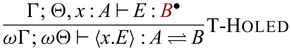
It is crucially important that x is added to the invertible environment. Recall again that $\omega \Theta$
ensures
$\omega \Theta$
ensures $\Theta = {epsilon}$
. Also, since values are closed in terms of unidirectional variables, a value of the form
$\Theta = {epsilon}$
. Also, since values are closed in terms of unidirectional variables, a value of the form $\langle x. E \rangle$
cannot have any free variables.
$\langle x. E \rangle$
cannot have any free variables.
3.5.2 Three evaluation relations: Unidirectional, forward, and backward
The evaluation relations are shown in Figure 4, which are defined by mutually dependent evaluation rules.
Evaluation relations: unidirectional, forward and backward.

The unidirectional evaluation is rather standard, except that it treats invertible primitives (such as lifted constructors, invertible ${{{{\mathbf{case}}}}}$
s,
${{{{\mathbf{case}}}}}$
s, ${{{{\mathbf{lift}}}}}$
, and
${{{{\mathbf{lift}}}}}$
, and ${{{{\mathbf{pin}}}}}$
) as constructors. A subtlety is that we assume dynamic
${{{{\mathbf{pin}}}}}$
) as constructors. A subtlety is that we assume dynamic $\alpha$
-renaming of invertible
$\alpha$
-renaming of invertible ${{{{\mathbf{case}}}}}$
s to avoid variable capturing. The evaluation rules can evaluate open expressions by having
${{{{\mathbf{case}}}}}$
s to avoid variable capturing. The evaluation rules can evaluate open expressions by having $x \Downarrow x$
; recall that residuals can contain variables. The
$x \Downarrow x$
; recall that residuals can contain variables. The ${{{{\mathbf{unlift}}}}}$
operator uses a fresh variable y in the evaluation to make a single-holed residual
${{{{\mathbf{unlift}}}}}$
operator uses a fresh variable y in the evaluation to make a single-holed residual $\langle y. E \rangle$
as a representation of bijection. Such single-holed residuals can be used in the forward direction by
$\langle y. E \rangle$
as a representation of bijection. Such single-holed residuals can be used in the forward direction by $e_1 \triangleright e_2$
and in the backward direction by
$e_1 \triangleright e_2$
and in the backward direction by $e_1 \triangleleft e_2$
, by triggering the corresponding evaluation.
$e_1 \triangleleft e_2$
, by triggering the corresponding evaluation.
The forward evaluation $\mu \vdash E \Rightarrow v$
states that under environment
$\mu \vdash E \Rightarrow v$
states that under environment $\mu$
, a residual E evaluates to a value v, and the backward evaluation
$\mu$
, a residual E evaluates to a value v, and the backward evaluation $E \Leftarrow v \dashv \mu$
inversely evaluates E to return the environment
$E \Leftarrow v \dashv \mu$
inversely evaluates E to return the environment $\mu$
from a value v: the forward and backward evaluation relations form a bijection. For variables and invertible constructors, both forward and backward evaluation rules are rather straightforward. The rules for invertible
$\mu$
from a value v: the forward and backward evaluation relations form a bijection. For variables and invertible constructors, both forward and backward evaluation rules are rather straightforward. The rules for invertible ${{{{\mathbf{case}}}}}$
expression are designed to ensure that every branch taken in one direction may and must be taken in the other direction too. This is why we check the
${{{{\mathbf{case}}}}}$
expression are designed to ensure that every branch taken in one direction may and must be taken in the other direction too. This is why we check the $\mathrel{{{{{\mathbf{with}}}}}}$
conditions even in the forward evaluation: the condition is considered as a post-condition that must exclusively hold after the evaluation of a branch. The
$\mathrel{{{{{\mathbf{with}}}}}}$
conditions even in the forward evaluation: the condition is considered as a post-condition that must exclusively hold after the evaluation of a branch. The ${{{{\mathbf{pin}}}}}$
operator changes the behavior of the backward computation of the second argument based on the result of the first argument; notice that
${{{{\mathbf{pin}}}}}$
operator changes the behavior of the backward computation of the second argument based on the result of the first argument; notice that $v_1$
, the parameter for the second argument, is obtained as the evaluation result of the first argument in the forward evaluation, and as the first component of the result pair in the backward evaluation. Notice that the unidirectional evaluation
$v_1$
, the parameter for the second argument, is obtained as the evaluation result of the first argument in the forward evaluation, and as the first component of the result pair in the backward evaluation. Notice that the unidirectional evaluation ![]() involved in the presented evaluation rules is performed in the same way in both evaluation, which is the key to bijectivity of E.
involved in the presented evaluation rules is performed in the same way in both evaluation, which is the key to bijectivity of E.
3.6 Metatheory
In this subsection, we present the key properties about ${{{{\lambda^{\mathrm{PI}}_{\to}}}}}$
.
${{{{\lambda^{\mathrm{PI}}_{\to}}}}}$
.
3.6.1 Subject reduction
First, we show a substitution lemma for ${{{{\lambda^{\mathrm{PI}}_{\to}}}}}$
. We only need to consider substitution for unidirectional variables because substitution for invertible variables never happens in evaluation; recall that we use environments (
${{{{\lambda^{\mathrm{PI}}_{\to}}}}}$
. We only need to consider substitution for unidirectional variables because substitution for invertible variables never happens in evaluation; recall that we use environments ( $\mu$
) in the forward and backward evaluation.
$\mu$
) in the forward and backward evaluation.
Lemma 3.1 $\Gamma, x :_\pi A ; \Theta \vdash e : B$
and
$\Gamma, x :_\pi A ; \Theta \vdash e : B$
and $\Gamma'; \Theta' \vdash e' : A$
implies
$\Gamma'; \Theta' \vdash e' : A$
implies $\Gamma + \pi \Gamma'; \Theta + \pi \Theta' \vdash e[e'/x] : B$
.
$\Gamma + \pi \Gamma'; \Theta + \pi \Theta' \vdash e[e'/x] : B$
.
Note that the substitution is only valid when $\Theta + \pi \Theta'$
satisfy the assumption that invertible variables have multiplicity 1. This assumption is guaranteed by typing of the constructs that trigger substitution.
$\Theta + \pi \Theta'$
satisfy the assumption that invertible variables have multiplicity 1. This assumption is guaranteed by typing of the constructs that trigger substitution.
Then, by Lemma 3.1, we have the subject reduction properties as follows:
Lemma 3.2 (subject reduction). The following properties hold:
-
Suppose
${epsilon}; \Theta \vdash e : A$
and
$e \Downarrow v$
. Then,
${epsilon}; \Theta \vdash v : A$
holds. -
Suppose
and
$\mu \vdash E \Rightarrow v$
. Then,
$\mathsf{dom}(\Theta) = \mathsf{dom}(\mu)$
holds, and
${epsilon}; {epsilon} \vdash \mu(x) : \Theta(x)$
for all
$x \in \mathsf{dom}(\Theta)$
implies
${epsilon}; {epsilon} \vdash v : A$
. -
Suppose
and
$E \Leftarrow v \dashv \mu$
. Then,
$\mathsf{dom}(\Theta) = \mathsf{dom}(\mu)$
holds, and
${epsilon}; {epsilon} \vdash v : A$
implies
${epsilon}; {epsilon} \vdash \mu(x) : \Theta(x)$
for all
$x \in \mathsf{dom}(\Theta)$
.Proof. By (mutual) induction on the derivation steps of evaluation.


The statements correspond to the three evaluation relations in ${{{{\lambda^{\mathrm{PI}}_{\to}}}}}$
. Note that the unidirectional evaluation targets expressions that are closed in terms of unidirectional variables, but may be open in terms of invertible variables, a property that is reflected in the first statement above. The second and third statements are more standard, assuming closed expressions in terms of both unidirectional and invertible variables. This assumption is actually an invariant; even though open expressions and values are involved in the unidirectional evaluation, the forward and backward evaluations always take and return closed values.
${{{{\lambda^{\mathrm{PI}}_{\to}}}}}$
. Note that the unidirectional evaluation targets expressions that are closed in terms of unidirectional variables, but may be open in terms of invertible variables, a property that is reflected in the first statement above. The second and third statements are more standard, assuming closed expressions in terms of both unidirectional and invertible variables. This assumption is actually an invariant; even though open expressions and values are involved in the unidirectional evaluation, the forward and backward evaluations always take and return closed values.
3.6.2 Bijectivity
Roughly speaking, correctness means that every value of type ${A \rightleftharpoons B}$
forms a bijection. Values of type
${A \rightleftharpoons B}$
forms a bijection. Values of type ${A \rightleftharpoons B}$
has the form
${A \rightleftharpoons B}$
has the form $\langle x. E \rangle$
. By Lemma 3.2 and T-Holed, values that occur in the evaluation of a well-typed term can be typed as
$\langle x. E \rangle$
. By Lemma 3.2 and T-Holed, values that occur in the evaluation of a well-typed term can be typed as ${epsilon}; {epsilon} \vdash \langle x. E \rangle : {A \rightleftharpoons B}$
, which implies
${epsilon}; {epsilon} \vdash \langle x. E \rangle : {A \rightleftharpoons B}$
, which implies ![]() . Since values
. Since values $\langle x. E \rangle$
can only be used by
$\langle x. E \rangle$
can only be used by $ \triangleright $
and
$ \triangleright $
and $ \triangleleft $
, bijectivity is represented as:
$ \triangleleft $
, bijectivity is represented as: ${ x \mapsto v} \vdash E \Rightarrow v'$
if and only if
${ x \mapsto v} \vdash E \Rightarrow v'$
if and only if $E \Leftarrow v' \dashv {x \mapsto v}$
.Footnote
13
$E \Leftarrow v' \dashv {x \mapsto v}$
.Footnote
13
To do so, we prove the following more general correspondence between the forward and backward evaluation relations, which is rather straightforward as the rules of the two evaluations are designed to be symmetric.
Lemma 3.3
(bijectivity of residuals). $\mu \vdash E \Rightarrow v$
if and only if
$\mu \vdash E \Rightarrow v$
if and only if $E \Leftarrow v \dashv \mu$
.
$E \Leftarrow v \dashv \mu$
.
Proof. Each direction is proved by induction on a derivation of the corresponding evaluation. Note that every unidirectional evaluation judgment $e' \Downarrow v'$
occurring in a derivation of one direction also appears in the corresponding derivation of the other direction, and hence we can treat the unidirectional evaluation as a block box in this proof.
$e' \Downarrow v'$
occurring in a derivation of one direction also appears in the corresponding derivation of the other direction, and hence we can treat the unidirectional evaluation as a block box in this proof.
Then, by Lemma 3.2, we have the following corollary stating that $\langle x. E \rangle : {A \rightleftharpoons B}$
actually implements a bijection between A-typed values and B-typed values.
$\langle x. E \rangle : {A \rightleftharpoons B}$
actually implements a bijection between A-typed values and B-typed values.
Corollary 3.4
(bijectivity of bijection values). Suppose ${epsilon}; {epsilon} \vdash \langle x. E \rangle : {A \rightleftharpoons B}$
. Then, for any v and u such that
${epsilon}; {epsilon} \vdash \langle x. E \rangle : {A \rightleftharpoons B}$
. Then, for any v and u such that ${epsilon}; {epsilon} \vdash v : A$
and
${epsilon}; {epsilon} \vdash v : A$
and ${epsilon}; {epsilon} \vdash v' : B$
, we have
${epsilon}; {epsilon} \vdash v' : B$
, we have ${x \mapsto v} \vdash E \Rightarrow v'$
if and only if
${x \mapsto v} \vdash E \Rightarrow v'$
if and only if $E \Leftarrow v' \dashv {x \mapsto v}$
.
$E \Leftarrow v' \dashv {x \mapsto v}$
.
3.6.3 Note on the progress property
Progress is another important property that, together with subjection reduction, proves the absence of certain errors during evaluation. However, a standard progress property is usually based on small-step semantics, and yet ${{{{\lambda^{\mathrm{PI}}_{\to}}}}}$
has a big-step operational semantics, which was chosen for its advantage in clarifying the input-output relationship of the forward and backward evaluation, as demonstrated by Lemma 3.3. A standard small-step semantics, which defines one-step evaluation as a relation between terms, is not suitable in this regard. Abstract machines are also unsatisfactory, as they will obscure the correspondence between the forward and backward evaluations.
${{{{\lambda^{\mathrm{PI}}_{\to}}}}}$
has a big-step operational semantics, which was chosen for its advantage in clarifying the input-output relationship of the forward and backward evaluation, as demonstrated by Lemma 3.3. A standard small-step semantics, which defines one-step evaluation as a relation between terms, is not suitable in this regard. Abstract machines are also unsatisfactory, as they will obscure the correspondence between the forward and backward evaluations.
We instead establish progress by directly showing that the evaluations do not get stuck other than with branching-related errors. This is done as an Agda implementation (mentioned in Sections 1 and 2.7) of definitional (Reynolds, Reference Reynolds1998) interpreters, which use the (sized) delay monad (Capretta, Reference Capretta2005; Abel & Chapman, Reference Abel and Chapman2014) and manipulate intrinsically typed (i.e., Church style) expressions, values, and residuals. The interpreter uses sums, products, and iso-recursive types instead of constructors. Also, instead of substitution, value environments are used in the unidirectional evaluation to avoid the shifting of de Bruijn terms. See Section 4 for details of the implementation. We note that, as a bonus track, the Agda implementation comes with a formal proof of Lemma 3.3.
3.6.4 Reversible Turing completeness
Reversible Turing completeness (Bennett, Reference Bennett1973) is an important property that general-purpose reversible languages are expected to have. Similar to the standard Turing completeness, being reversible Turing complete for a language means that all bijections can be expressed in the language (Bennett, Reference Bennett1973).
It is unsurprising that ${{{{\lambda^{\mathrm{PI}}_{\to}}}}}$
is reversible Turing complete, as it has recursion (via
${{{{\lambda^{\mathrm{PI}}_{\to}}}}}$
is reversible Turing complete, as it has recursion (via ${fix}_\pi$
in Section 3.3) and reversible branching (i.e., invertible
${fix}_\pi$
in Section 3.3) and reversible branching (i.e., invertible ${{{{\mathbf{case}}}}}$
).
${{{{\mathbf{case}}}}}$
).
Theorem 3.5 ${{{{\lambda^{\mathrm{PI}}_{\to}}}}}$
is reversible Turing complete.
${{{{\lambda^{\mathrm{PI}}_{\to}}}}}$
is reversible Turing complete.
The proof is done by constructing a simulator for a given reversible Turing machine, which is presented in Appendix A. We follow the construction in Yokoyama et al. (Reference Yokoyama, Axelsen and Glück2011)except the last step, in which we use a general reversible looping operator as below.Footnote 14
As its type suggests, ${trace} ~ h$
applies h to
${trace} ~ h$
applies h to $\mathsf{InL} ~ a$
repeatedly until it returns
$\mathsf{InL} ~ a$
repeatedly until it returns $\mathsf{InL} ~ b$
; the function loops while h returns a value of the form
$\mathsf{InL} ~ b$
; the function loops while h returns a value of the form $\mathsf{InR} ~ x$
. Intuitively, this behavior corresponds to the reversible loop (Lutz, Reference Lutz1986). In functional programming, loops are naturally encoded as tail recursions, which, however, are known to be difficult to handle in the contexts of program inversion (Glück & Kawabe, Reference Glück and Kawabe2004; Mogensen, Reference Mogensen, Virbitskaite and Voronkov2006; Matsuda et al., Reference Matsuda, Mu, Hu and Takeichi2010; Nishida & Vidal, Reference Nishida and Vidal2011). In fact, our implementation uses a non-trivial reversible programming technique, namely Yokoyama et al. (2012)’s optimized version of Bennett (Reference Bennett1973)’s encoding. The higher-orderness of
$\mathsf{InR} ~ x$
. Intuitively, this behavior corresponds to the reversible loop (Lutz, Reference Lutz1986). In functional programming, loops are naturally encoded as tail recursions, which, however, are known to be difficult to handle in the contexts of program inversion (Glück & Kawabe, Reference Glück and Kawabe2004; Mogensen, Reference Mogensen, Virbitskaite and Voronkov2006; Matsuda et al., Reference Matsuda, Mu, Hu and Takeichi2010; Nishida & Vidal, Reference Nishida and Vidal2011). In fact, our implementation uses a non-trivial reversible programming technique, namely Yokoyama et al. (2012)’s optimized version of Bennett (Reference Bennett1973)’s encoding. The higher-orderness of ${{{{\lambda^{\mathrm{PI}}_{\to}}}}}$
(and Sparcl) helps here, as the effort is made once and for all.
${{{{\lambda^{\mathrm{PI}}_{\to}}}}}$
(and Sparcl) helps here, as the effort is made once and for all.
3.7 Extension with the
${{{{{\mathbf{lift}}}}}}$
operator

One feature we have not yet discussed is the ${{{{\mathbf{lift}}}}}$
operator that creates primitive bijections from unidirectional programs, for example, sub as we have seen in Section 2.
${{{{\mathbf{lift}}}}}$
operator that creates primitive bijections from unidirectional programs, for example, sub as we have seen in Section 2.
Adding ${{{{\mathbf{lift}}}}}$
to
${{{{\mathbf{lift}}}}}$
to ${{{{\lambda^{\mathrm{PI}}_{\to}}}}}$
is rather easy. We extend expressions to include
${{{{\lambda^{\mathrm{PI}}_{\to}}}}}$
is rather easy. We extend expressions to include ${{{{\mathbf{lift}}}}}$
as
${{{{\mathbf{lift}}}}}$
as ![]()
![]() together with the following typing rule.
together with the following typing rule.

Accordingly, we extend evaluation by adding residuals of the form ${{{{\mathbf{lift}}}}} ~ (\lambda_\omega x_1.e_1)$ $~ (\lambda_\omega x_2.e_2) ~ E_3$
together with the following forward and backward evaluation rules (we omit the obvious unidirectional evaluation rule for obtaining residuals of this form).
$~ (\lambda_\omega x_2.e_2) ~ E_3$
together with the following forward and backward evaluation rules (we omit the obvious unidirectional evaluation rule for obtaining residuals of this form).

The substitution lemma (Lemma 3.1) and the subject reduction properties (Lemma 3.2) are also lifted to ${{{{\mathbf{lift}}}}}$
.
${{{{\mathbf{lift}}}}}$
.
However, ${{{{\mathbf{lift}}}}}$
is by nature unsafe, which requires an additional condition to ensure correctness. Specifically, the bijectivity of
${{{{\mathbf{lift}}}}}$
is by nature unsafe, which requires an additional condition to ensure correctness. Specifically, the bijectivity of ${A \rightleftharpoons B}$
-typed values is only guaranteed if
${A \rightleftharpoons B}$
-typed values is only guaranteed if ${{{{\mathbf{lift}}}}}$
is used for pairs of functions that actually form bijections. For example, the uses of
${{{{\mathbf{lift}}}}}$
is used for pairs of functions that actually form bijections. For example, the uses of ${{{{\mathbf{lift}}}}}$
to construct sub in Section 2 are indeed safe. In Section 5.2.1, we will see another interesting example showing the use of conditionally safe
${{{{\mathbf{lift}}}}}$
to construct sub in Section 2 are indeed safe. In Section 5.2.1, we will see another interesting example showing the use of conditionally safe ${{{{\mathbf{lift}}}}}$
s (see unsafeNew in Section 5.2.1).
${{{{\mathbf{lift}}}}}$
s (see unsafeNew in Section 5.2.1).
4 Mechanized proof in Agda
In this section, we provide an overview of our implementation of Sparcl in Adga which serves as a witness of the subjection reduction and the progress properties. Also, the implementation establish the invariant that the multiplicities of the variables in $\Theta$
are always 1. This is crucial for the correctness but non-trivial to establish in our setting, because an expression and the value obtained as the evaluation result of the expression may have different free invertible variables due to the unidirectional free variables in the expression. The Agda implementation also comes with the proof of Lemma 3.3.
$\Theta$
are always 1. This is crucial for the correctness but non-trivial to establish in our setting, because an expression and the value obtained as the evaluation result of the expression may have different free invertible variables due to the unidirectional free variables in the expression. The Agda implementation also comes with the proof of Lemma 3.3.
4.1 Differences in formalization
We first spell out the differences in our Agda formalization from the system ${{{{\lambda^{\mathrm{PI}}_{\to}}}}}$
described in Section 3. As mentioned earlier, the implementation uses products, sums, and iso-recursive types instead of constructors and uses environments instead of substitutions to avoid tedious shifting of de Bruijn terms. In addition, the Agda version comes with a slight extension to support
${{{{\lambda^{\mathrm{PI}}_{\to}}}}}$
described in Section 3. As mentioned earlier, the implementation uses products, sums, and iso-recursive types instead of constructors and uses environments instead of substitutions to avoid tedious shifting of de Bruijn terms. In addition, the Agda version comes with a slight extension to support $!$
in linear calculi.
$!$
in linear calculi.
We begin with the difference in types. The Agda version targets the following set of types.
As one can see, there are no user-defined types ![]() that come with constructors; instead, we have the unit type (), product types
that come with constructors; instead, we have the unit type (), product types $A \otimes B$
, sum types
$A \otimes B$
, sum types $A \oplus B$
, and (iso-) recursive types
$A \oplus B$
, and (iso-) recursive types $\mu \alpha. A$
. As for the extension mentioned earlier, there are also types of the form of
$\mu \alpha. A$
. As for the extension mentioned earlier, there are also types of the form of $!{\pi}{A}$
which intuitively denote A-typed values together with the witness of
$!{\pi}{A}$
which intuitively denote A-typed values together with the witness of $\pi$
-many copyability of the values.
$\pi$
-many copyability of the values.
The expressions are updated to match the types.
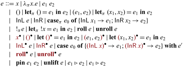
Instead of constructors and pattern matching, this version includes the introduction and elimination forms for each form of types except ![]() . And for types (),
. And for types (), $A \otimes B$
,
$A \otimes B$
, $A \oplus B$
, and
$A \oplus B$
, and $\mu \alpha. A$
, there are corresponding invertible versions. For example, we have the introduction form
$\mu \alpha. A$
, there are corresponding invertible versions. For example, we have the introduction form $(e_1,e_2)$
and the elimination form
$(e_1,e_2)$
and the elimination form ${{{{\mathbf{let}}}}}_\pi~(x_1,x_2) = e_1~{{{{\mathbf{in}}}}}~e_2$
for the product types, and their invertible counterparts
${{{{\mathbf{let}}}}}_\pi~(x_1,x_2) = e_1~{{{{\mathbf{in}}}}}~e_2$
for the product types, and their invertible counterparts ![]() . Here,
. Here, $\pi$
ensures that
$\pi$
ensures that $e_1$
is used
$e_1$
is used $\pi$
-many times and so as the variables
$\pi$
-many times and so as the variables $x_1$
and
$x_1$
and $x_2$
, similarly to the
$x_2$
, similarly to the $\pi$
of
$\pi$
of ${{{{\mathbf{case}}}}}_\pi$
in the original calculus
${{{{\mathbf{case}}}}}_\pi$
in the original calculus ${{{{\lambda^{\mathrm{PI}}_{\to}}}}}$
(see T-Case in Figure 3). Note that both (unidirectional and invertible) sorts of
${{{{\lambda^{\mathrm{PI}}_{\to}}}}}$
(see T-Case in Figure 3). Note that both (unidirectional and invertible) sorts of ${{{{\mathbf{case}}}}}$
s are only for sum types and have exactly two branches. For simplicity, the invertible
${{{{\mathbf{case}}}}}$
s are only for sum types and have exactly two branches. For simplicity, the invertible ${{{{\mathbf{case}}}}}$
has one
${{{{\mathbf{case}}}}}$
has one $\mathrel{{{{{\mathbf{with}}}}}}$
condition instead of two, as one is enough to select one of the two branches. Since we use intrinsically typed terms, the syntax of terms must be designed so that the typing relation becomes syntax-directed. Hence, we have two sorts of variable expressions (not variables themselves) x and
$\mathrel{{{{{\mathbf{with}}}}}}$
condition instead of two, as one is enough to select one of the two branches. Since we use intrinsically typed terms, the syntax of terms must be designed so that the typing relation becomes syntax-directed. Hence, we have two sorts of variable expressions (not variables themselves) x and ![]() , which will be typed by T-Var and T-RVar, respectively.
, which will be typed by T-Var and T-RVar, respectively.
The typing rules for the expressions can be obtained straightforwardly from Figure 3, except for the newly introduced ones that manipulate $!{\pi}{A}$
-typed values.
$!{\pi}{A}$
-typed values.

An intuition underlying the rules is that $!{\pi}{A}$
is treated as a GADT (
$!{\pi}{A}$
is treated as a GADT ( $\mathsf{Many} ~ \pi ~ A$
) with the constructor
$\mathsf{Many} ~ \pi ~ A$
) with the constructor $\mathsf{MkMany} : A \multimap_\pi \mathsf{Many} ~ {\pi} ~ {A}$
capturing the multiplicity
$\mathsf{MkMany} : A \multimap_\pi \mathsf{Many} ~ {\pi} ~ {A}$
capturing the multiplicity $\pi$
. As the constructor discharges the multiplicity
$\pi$
. As the constructor discharges the multiplicity $\pi$
when pattern matched, the latter rule says that the copyability
$\pi$
when pattern matched, the latter rule says that the copyability $\pi_1$
is discharged by the binding, regardless of the use of the examined expression
$\pi_1$
is discharged by the binding, regardless of the use of the examined expression $e_1$
. For example, we have
$e_1$
. For example, we have $x :_1 (), y :_\omega A ; {epsilon} \vdash {{{{\mathbf{let}}}}}_1~!{}{z} = ({{{{\mathbf{let}}}}}_1~() = x~{{{{\mathbf{in}}}}}~!{\omega}{y})~{{{{\mathbf{in}}}}}~(z,z) : A \otimes A$
where x is used once in the expression but z can be used twice as the binding discharged the copyability witnessed by
$x :_1 (), y :_\omega A ; {epsilon} \vdash {{{{\mathbf{let}}}}}_1~!{}{z} = ({{{{\mathbf{let}}}}}_1~() = x~{{{{\mathbf{in}}}}}~!{\omega}{y})~{{{{\mathbf{in}}}}}~(z,z) : A \otimes A$
where x is used once in the expression but z can be used twice as the binding discharged the copyability witnessed by $!{\omega}{y}$
.
$!{\omega}{y}$
.
The sets of values and residuals are also updated accordingly. Here, the main change is the use of environments ![]() .
.
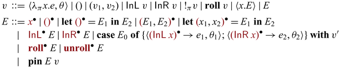
We intentionally used different metavariables $\theta$
and
$\theta$
and $\mu$
for environments: the former is used in the unidirectional evaluation and may contain invertible free variables, while the latter is used in the forward and backward evaluations. The typing relation
$\mu$
for environments: the former is used in the unidirectional evaluation and may contain invertible free variables, while the latter is used in the forward and backward evaluations. The typing relation $\Theta \vdash \theta : \Gamma$
must be aware of such free invertible variables as below.
$\Theta \vdash \theta : \Gamma$
must be aware of such free invertible variables as below.

The typing rules for values and residuals ( $\Theta \vdash v : A$
and
$\Theta \vdash v : A$
and ![]() ) are obtained straightforwardly from the rules for expressions (Figure 3) with
) are obtained straightforwardly from the rules for expressions (Figure 3) with $\Gamma = {epsilon}$
, except for the two new forms of value and residual involving closures. One of the two is a function closure expression
$\Gamma = {epsilon}$
, except for the two new forms of value and residual involving closures. One of the two is a function closure expression $\langle \lambda x_\pi. e, \theta \rangle$
, which comes with the following typing rule.
$\langle \lambda x_\pi. e, \theta \rangle$
, which comes with the following typing rule.
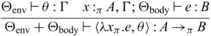
The other is the invertible ${{{{\mathbf{case}}}}}$
residual, which has the following type rule.
${{{{\mathbf{case}}}}}$
residual, which has the following type rule.

Here, we write $\mathsf{Bool}$
for
$\mathsf{Bool}$
for $() \oplus ()$
for readability.
$() \oplus ()$
for readability.
We omit the concrete representations of expressions, values, and residuals as they are straightforward. A subtlety is that the Agda version adopts separate treatment of types and multiplicities: that is, $\Gamma = \{ x_1 :_{\pi_1} A_1,\dots, x_n :_{\pi_n} A_n\}$
is separated into
$\Gamma = \{ x_1 :_{\pi_1} A_1,\dots, x_n :_{\pi_n} A_n\}$
is separated into $\Gamma_\mathrm{t} = \{x_1 : A_1,\dots, x_n : A_n \}$
and
$\Gamma_\mathrm{t} = \{x_1 : A_1,\dots, x_n : A_n \}$
and $\Gamma_\mathrm{m} = \{x_1 : \pi_1,\dots, x_n : \pi_n \}$
, so that complex manipulation of multiplicities happens only for the latter. Also,
$\Gamma_\mathrm{m} = \{x_1 : \pi_1,\dots, x_n : \pi_n \}$
, so that complex manipulation of multiplicities happens only for the latter. Also, $\Theta$
environments are separated into
$\Theta$
environments are separated into $\Theta_\mathrm{t}$
and
$\Theta_\mathrm{t}$
and $\Theta_\mathrm{m}$
in a similar way.
$\Theta_\mathrm{m}$
in a similar way.
4.2 Evaluation functions
The Agda implementations include two definitional (Reynolds, Reference Reynolds1998) interpreters for intrinsically typed terms: one is for the unidirectional evaluation $\mathrel{\Downarrow}$
and the other is for the forward and backward evaluations
$\mathrel{\Downarrow}$
and the other is for the forward and backward evaluations $\mathrel{\Rightarrow}$
and
$\mathrel{\Rightarrow}$
and $\mathrel{\Leftarrow}$
. More specifically, the former one takes
$\mathrel{\Leftarrow}$
. More specifically, the former one takes $\Theta' \vdash \theta : \Gamma$
and
$\Theta' \vdash \theta : \Gamma$
and $\Gamma ; \Theta \vdash e : A$
to produce a value
$\Gamma ; \Theta \vdash e : A$
to produce a value $\Theta' + \Theta \vdash v : A$
if terminates, and the latter takes a residual
$\Theta' + \Theta \vdash v : A$
if terminates, and the latter takes a residual ![]() to yield a not-necessarily-total bijection between
to yield a not-necessarily-total bijection between $\mu : \Theta$
and
$\mu : \Theta$
and $\vdash v : A$
, where
$\vdash v : A$
, where $\mu : \Theta$
means
$\mu : \Theta$
means $\vdash \mu(x) : \Theta(x)$
for any x.
$\vdash \mu(x) : \Theta(x)$
for any x.
In our Agda development, an environment-in-context $\Theta' \vdash \theta : \Gamma$
, a term-in-context
$\Theta' \vdash \theta : \Gamma$
, a term-in-context $\Gamma ; \Theta \vdash e : A$
, and a value-in-context
$\Gamma ; \Theta \vdash e : A$
, and a value-in-context $\Theta' + \Theta \vdash v : A$
are represented by types
$\Theta' + \Theta \vdash v : A$
are represented by types ![]() , respectively. Recall that we have adopted the separate treatment of types and multiplicities. Hence, instead of having a single
, respectively. Recall that we have adopted the separate treatment of types and multiplicities. Hence, instead of having a single $\Theta$
, we have
$\Theta$
, we have $\Theta_\mathrm{t}$
and
$\Theta_\mathrm{t}$
and $\Theta_\mathrm{m}$
where the former typing environment is treated in the usual way. Also, regarding the latter evaluation, a residual-in-context
$\Theta_\mathrm{m}$
where the former typing environment is treated in the usual way. Also, regarding the latter evaluation, a residual-in-context ![]() , a typed-environment (for the forward/backward evaluation)
, a typed-environment (for the forward/backward evaluation) $\mu : \Theta$
, and a value-in-context
$\mu : \Theta$
, and a value-in-context $\vdash v : A$
are represented by types
$\vdash v : A$
are represented by types ![]() , and
, and ![]() , respectively. The different representations
, respectively. The different representations ![]() are used for the empty typing environment and the empty multiplicity environment: the former type is just a list of types, while the latter is a type indexed by the former.
are used for the empty typing environment and the empty multiplicity environment: the former type is just a list of types, while the latter is a type indexed by the former.
Now, we are ready to give the signatures of the two evaluation functions.
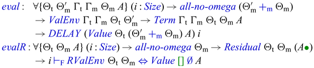
The predicate ![]() asserts that a given multiplicity environment does not contain the multiplicity
asserts that a given multiplicity environment does not contain the multiplicity $\omega$
, respecting the assumption on the core system that the multiplicities involved in
$\omega$
, respecting the assumption on the core system that the multiplicities involved in $\Theta$
are always 1. This property is considered as an invariant, because we need to have a witness of the property to call
$\Theta$
are always 1. This property is considered as an invariant, because we need to have a witness of the property to call ![]() recursively. The type constructor
recursively. The type constructor ![]() is a variant the (sized) delay monad (Capretta, Reference Capretta2005; Abel & Chapman, Reference Abel and Chapman2014), where the bind operation is frozen (i.e., represented as a constructor). This deviation from the original is useful for the proof of Lemma 3.3 (Section 4.3). The record type
is a variant the (sized) delay monad (Capretta, Reference Capretta2005; Abel & Chapman, Reference Abel and Chapman2014), where the bind operation is frozen (i.e., represented as a constructor). This deviation from the original is useful for the proof of Lemma 3.3 (Section 4.3). The record type ![]() represents not-necessarily-total bijections and has two fields:
represents not-necessarily-total bijections and has two fields: ![]() and
and ![]() .
.
The fact that we have implemented these two functions in Agda witnesses the subject reduction and the progress property. For the two functions to be type correct, they must use appropriate recursive calls for intrinsically typed subterms, which is indeed what the subject reduction requires. Also, Agda is a total language, meaning that we need to give the definition for every possible structures—in other words, every typed term is subject to evaluation. Note that, by ![]() , the evaluations are allowed to go into infinite loops, which is legitate for the progress property. We also use infinite loops to represent errors, which are thrown only in the following situations.
, the evaluations are allowed to go into infinite loops, which is legitate for the progress property. We also use infinite loops to represent errors, which are thrown only in the following situations.
-
forward evaluation of invertible
${{{{\mathbf{case}}}}}$
s with imprecise
$\mathrel{{{{{\mathbf{with}}}}}}$
conditions, and -
backward evaluation of
that receive opposite values.


The fact that the interpreters are typechecked in Agda serves as a constructive proof that there are no other kind of errors.
Caveat: sized types.
As their signatures suggest, the definitions of ![]() rely on (a variant of) the sized delay monad. However, the sized types are in fact an unsafe feature in Agda 2.6.2, which may lead to contradictions in cases,Footnote
15
and, as far as we are aware, the safe treatment of sized types is still open in Agda. Nevertheless, we believe that our use of sized types, mainly regarding sized delay monads, is safe as the use is rather standard (namely, we use the finite sized types in the definitions of
rely on (a variant of) the sized delay monad. However, the sized types are in fact an unsafe feature in Agda 2.6.2, which may lead to contradictions in cases,Footnote
15
and, as far as we are aware, the safe treatment of sized types is still open in Agda. Nevertheless, we believe that our use of sized types, mainly regarding sized delay monads, is safe as the use is rather standard (namely, we use the finite sized types in the definitions of ![]() to ensure productivity, and then use the infinite size when we discuss the property of the computation).
to ensure productivity, and then use the infinite size when we discuss the property of the computation).
4.3 Bijectivity of the forward and backward evaluation
The statement of Lemma 3.3 is formalized in Agda as the signatures of the following functions:
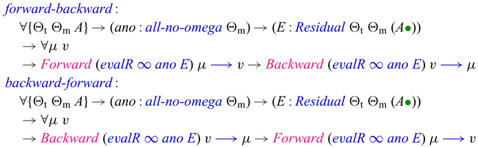
Here, ![]() , which reads that m evaluates to v, is an inductively defined predicate asserting that
, which reads that m evaluates to v, is an inductively defined predicate asserting that ![]() terminates and produces the final outcome v. This relation has a similar role to
terminates and produces the final outcome v. This relation has a similar role to ![]() are defined in the module Codata.Sized.Delay in the Agda standard library, but the key difference is its explicit bind structures. Thanks to the explicit bind structures, we can perform the proof straightforwardly by induction on E and case analysis on
are defined in the module Codata.Sized.Delay in the Agda standard library, but the key difference is its explicit bind structures. Thanks to the explicit bind structures, we can perform the proof straightforwardly by induction on E and case analysis on ![]()
![]() , leveraging the fact that the forward/backward evaluation “mirrors” the backward/forward evaluation also in the bind structures.
, leveraging the fact that the forward/backward evaluation “mirrors” the backward/forward evaluation also in the bind structures.
5 Larger examples
In this section, we demonstrate the utility of Sparcl with four examples, in which partial invertibility supported by Sparcl is the key for programming. The first one is rebuilding trees from preorder and inorder traversals (Mu & Bird, Reference Mu and Bird2003), and the latter three are simplified versions of compression algorithms (Salomon, Reference Salomon2008), namely, the Huffman coding, arithmetic coding, and LZ77 (Ziv & Lempel, Reference Ziv and Lempel1977).Footnote 16
5.1 Rebuilding trees from a preorder and an inorder traversals
It is well known that we can rebuild a node-labeled binary tree from its preorder and inorder traversals, provided that all labels in the tree are distinct. That is, for binary trees of type
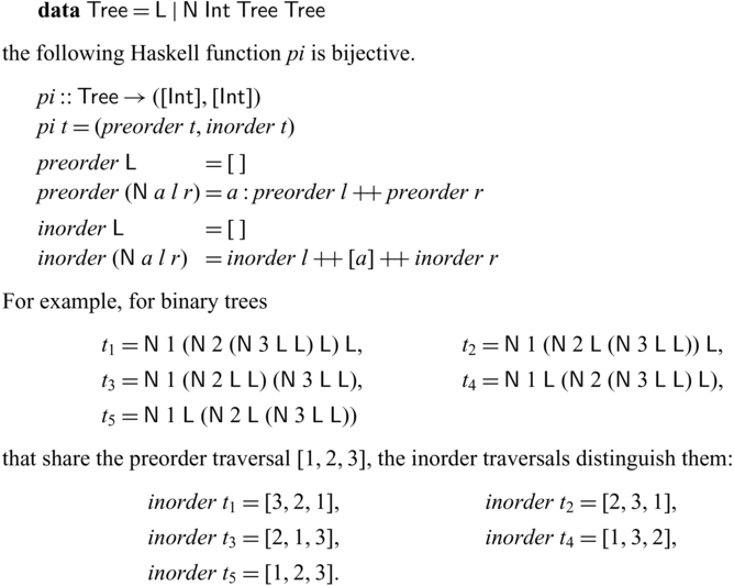
The uniqueness of labels is key to the bijectivity of pi. It is clear that ${pi}^{-1}$
returns
${pi}^{-1}$
returns $\mathsf{L}$
for
$\mathsf{L}$
for $({[\,]}, {[\,]})$
, so the nontrivial part is how
$({[\,]}, {[\,]})$
, so the nontrivial part is how ${pi}^{-1}$
will do for a pair of nonempty lists. Let us write
${pi}^{-1}$
will do for a pair of nonempty lists. Let us write $(a : {p}, i)$
for the pair. Then, since i contains exactly one a, we can unambiguously split i as
$(a : {p}, i)$
for the pair. Then, since i contains exactly one a, we can unambiguously split i as $i = i_1 \mathbin{+\!+} [a] \mathbin{+\!+} i_2$
. Then, by
$i = i_1 \mathbin{+\!+} [a] \mathbin{+\!+} i_2$
. Then, by ${pi}^{-1}({take} ~ ({length} ~ i_1) ~ {p}, i_1)$
, we can recover the left child l, and, by
${pi}^{-1}({take} ~ ({length} ~ i_1) ~ {p}, i_1)$
, we can recover the left child l, and, by ${pi}^{-1}({drop} ~ ({length} ~ i_1) ~ {p}, i_2)$
, we can recover the right child r. After that, from a, l, and r, we can construct the original input as
${pi}^{-1}({drop} ~ ({length} ~ i_1) ~ {p}, i_2)$
, we can recover the right child r. After that, from a, l, and r, we can construct the original input as $\mathsf{N} ~ a ~ l ~ r$
. Notice that this inverse computation already involves partial invertibility such as the splitting of the inorder traversal list based on a, which is invertible for fixed a with the uniqueness assumption.
$\mathsf{N} ~ a ~ l ~ r$
. Notice that this inverse computation already involves partial invertibility such as the splitting of the inorder traversal list based on a, which is invertible for fixed a with the uniqueness assumption.
It is straightforward to implement the above procedure in Sparcl. However, such a program is inefficient due to the cost of splitting. Program calculation is an established technique for deriving efficient programs through equational reasoning (Gibbons, Reference Gibbons, Backhouse, Crole and Gibbons2002), and in this case of tree-rebuilding, it is known that a linear-time inverse exists and can be derived (Mu & Bird, Reference Mu and Bird2003).
In the following, we demonstrate that program calculation works well in the setting of Sparcl. Interestingly, thinking in terms of partial-invertibility not only produces a Sparcl program, but actually improves the calculation by removing some of the more-obscure steps. Our calculation presented below basically follows Mu & Bird (Reference Mu and Bird2003, Section 3), although the presentation is a bit different as we focus on partial invertibility, especially the separation of unidirectional and invertible computation.
Note that Glück & Yokoyama (Reference Glück and Yokoyama2019) give a reversible version of tree rebuilding using (an extension of) R-WHILE (Glück & Yokoyama, Reference Glück and Yokoyama2016), a reversible imperative language inspired by Janus (Lutz, Reference Lutz1986; Yokoyama et al., Reference Yokoyama, Axelsen and Glück2008). However, R-WHILE only supports a very limited form of partial invertibility (Section 6.1), and the difference between their definition and ours is similar to what is demonstrated by the goSubs and goSubsF examples in Figure 2.
5.1.1 Calculation of the original definition
The first step is tupling (Chin, Reference Chin1993; Hu et al., Reference Hu, Iwasaki, Takeichi and Takano1997) which eliminates multiple data traversals. The elimination of multiple data traversals is known to be useful for program inversion (Eppstein, Reference Eppstein1985; Matsuda et al., Reference Matsuda, Inaba and Nakano2012).
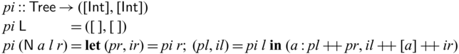
Mu & Bird (Reference Mu and Bird2003, Section 3) also use tupling as the first step in their derivation. The next step is to eliminate $\mathbin{+\!+}$
, a source of inefficiency. The standard technique is to use accumulation parameters (Kühnemann et al., Reference Kühnemann, Glück and Kakehi2001). Specifically, we obtain piA satisfying
$\mathbin{+\!+}$
, a source of inefficiency. The standard technique is to use accumulation parameters (Kühnemann et al., Reference Kühnemann, Glück and Kakehi2001). Specifically, we obtain piA satisfying ${piA} ~ t ~ {py} ~ {iy}= {{{{\mathbf{let}}}}}~(p,i) = {pi} ~ t~{{{{\mathbf{in}}}}}~(p \mathbin{+\!+} {py}, i \mathbin{+\!+} {iy})$
as below.
${piA} ~ t ~ {py} ~ {iy}= {{{{\mathbf{let}}}}}~(p,i) = {pi} ~ t~{{{{\mathbf{in}}}}}~(p \mathbin{+\!+} {py}, i \mathbin{+\!+} {iy})$
as below.
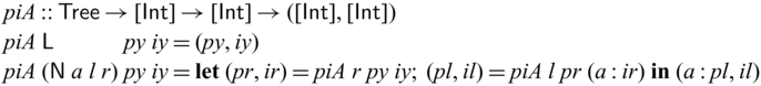
The invertibility of piA is still not clear because piA is called with two different forms of the accumulation parameter iy: one is the case where iy is empty (e.g., the initial call ${pi} ~ x = {piA} ~ x ~ {[\,]} ~ {[\,]}$
), and the other is the case where it is not (e.g., the recursion for the left child
${pi} ~ x = {piA} ~ x ~ {[\,]} ~ {[\,]}$
), and the other is the case where it is not (e.g., the recursion for the left child ${piA} ~ l ~ {pr} ~ (a : {ir})$
). This distinction between the two is important because, unlike the former, an inverse for the latter is responsible for searching for the appropriate place to separate the inorder-traversal list. Nevertheless, this separation can be achieved by deriving a specialized version pi of piA satisfying
${piA} ~ l ~ {pr} ~ (a : {ir})$
). This distinction between the two is important because, unlike the former, an inverse for the latter is responsible for searching for the appropriate place to separate the inorder-traversal list. Nevertheless, this separation can be achieved by deriving a specialized version pi of piA satisfying ${pi} ~ x = {piA} ~ x ~ {[\,]} ~ {[\,]}$
(we reuse the name as it implements the same function).
${pi} ~ x = {piA} ~ x ~ {[\,]} ~ {[\,]}$
(we reuse the name as it implements the same function).
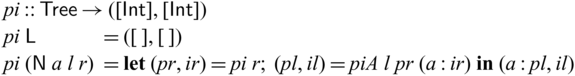
Having this new version of pi, we now have an invariant that iy of ${piA} ~ t ~ {py} ~ {iy}$
is always nonempty; the other case is separated into a call to pi. Moreover, we can determine the head h of iy beforehand in both forward and backward computations; this is exactly the label we search for to split the inorder-traversal list. Indeed, if we know the head h of iy beforehand, we can distinguish the ranges of the two branches of piA: for the first branch
${piA} ~ t ~ {py} ~ {iy}$
is always nonempty; the other case is separated into a call to pi. Moreover, we can determine the head h of iy beforehand in both forward and backward computations; this is exactly the label we search for to split the inorder-traversal list. Indeed, if we know the head h of iy beforehand, we can distinguish the ranges of the two branches of piA: for the first branch $({py}, {iy})$
, as iy is returned as is, the head of the second component is the same as h, and for the second branch
$({py}, {iy})$
, as iy is returned as is, the head of the second component is the same as h, and for the second branch $(a:{pl}, {il})$
, the head of the second component of the return value cannot be equal to h, i.e., the head of iy. Recall that
$(a:{pl}, {il})$
, the head of the second component of the return value cannot be equal to h, i.e., the head of iy. Recall that ${piA} ~ t ~ {py} ~ {iy}= {{{{\mathbf{let}}}}}~(p,i) = {pi} ~ t~{{{{\mathbf{in}}}}}~(p \mathbin{+\!+} {py}, i \mathbin{+\!+} {iy})$
; thus, ir in the definition of piA must have the form of
${piA} ~ t ~ {py} ~ {iy}= {{{{\mathbf{let}}}}}~(p,i) = {pi} ~ t~{{{{\mathbf{in}}}}}~(p \mathbin{+\!+} {py}, i \mathbin{+\!+} {iy})$
; thus, ir in the definition of piA must have the form of $\cdots \mathbin{+\!+} {iy}$
, and then il must have the form of
$\cdots \mathbin{+\!+} {iy}$
, and then il must have the form of $\cdots \mathbin{+\!+} [a] \mathbin{+\!+} \cdots \mathbin{+\!+} {iy}$
.
$\cdots \mathbin{+\!+} [a] \mathbin{+\!+} \cdots \mathbin{+\!+} {iy}$
.
Thus, as the last step of our calculation, we clarify the unidirectional part, namely the head of the second component of the accumulation parameters of piA, by changing it to a separate parameter. Specifically, we prepare the function piAS satisfying ${piAS} ~ h ~ t ~ {py} ~ {iy} = {piA} ~ t ~ {py} ~ (h : {iy})$
as below.
${piAS} ~ h ~ t ~ {py} ~ {iy} = {piA} ~ t ~ {py} ~ (h : {iy})$
as below.
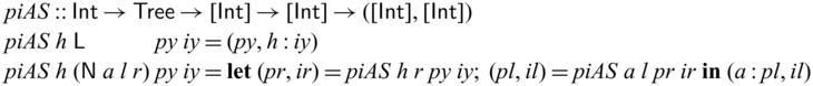
Also, we replace the function call of piA in pi appropriately.
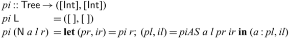
5.1.2 Making partial-invertibility explicit
An efficient implementation in Sparcl falls out from the above calculation (see Figure 5): the only additions are the types and the use of ${{{{\mathbf{pin}}}}}$
. Recall that
${{{{\mathbf{pin}}}}}$
. Recall that ![]() is syntactic sugar for
is syntactic sugar for ![]() . Recall also that the first match principle is assumed and the catch-all
. Recall also that the first match principle is assumed and the catch-all $\mathrel{{{{{\mathbf{with}}}}}}$
conditions for the second branches are omitted. The function new in the program lifts an A-typed value a to an
$\mathrel{{{{{\mathbf{with}}}}}}$
conditions for the second branches are omitted. The function new in the program lifts an A-typed value a to an ![]() -typed value, corresponding to a bijection between () and
-typed value, corresponding to a bijection between () and ${a}$
.
${a}$
.
Invertible pre- and in-order traversal in Sparcl.

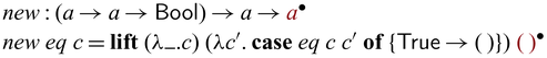
Note that the arguments of ${{{{\mathbf{lift}}}}}$
in
${{{{\mathbf{lift}}}}}$
in ${new} ~ {eq}$
form a not-necessarily-total bijection, provided that eq implements the equality on A.
${new} ~ {eq}$
form a not-necessarily-total bijection, provided that eq implements the equality on A.
The backward evaluation of piR has the same behavior as that Mu & Bird (Reference Mu and Bird2003, Section 3) derived. The partial bijection that piASR defines indeed corresponds to reb in their calculation. Their reb function is introduced as a rather magical step; our calculation can be seen as a justification of their choice.
5.1.3 new and delete
In the above example, we used new, which can be used to introduce redundancy to the output. For example, it is common to include checksum information in encoded data. The new function is effective for this scenario, as demonstrated below.
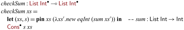
In the forward direction, checkSum computes the sum of the list and prepends it to the list. In the backward direction, it checks if the head of the input list is the sum of its tail: if the check succeeds, the backward computation of checkSum returns the tail, and (correctly) fails otherwise.
It is worth mentioning that the pattern ${new} ~ {eq}$
is a finer operation than reversible copying where the inverse is given by equivalence checking (Glück and Kawabe, Reference Glück and Kawabe2003); reversible copying can be implemented as
${new} ~ {eq}$
is a finer operation than reversible copying where the inverse is given by equivalence checking (Glück and Kawabe, Reference Glück and Kawabe2003); reversible copying can be implemented as ![]() , assuming appropriate
, assuming appropriate ${eq} : A \to A \to \mathsf{Bool}$
.
${eq} : A \to A \to \mathsf{Bool}$
.
The new function has the corresponding inverse delete, which can be used to remove redundancy from the input.
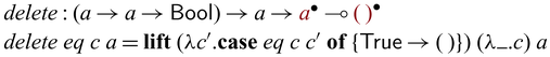
It is interesting to note that new and delete can be used to define a safe variant of ${{{{\mathbf{lift}}}}}$
.
${{{{\mathbf{lift}}}}}$
.
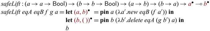
In the forward computation, the function applies f to the input and tests whether g is an inverse of f by applying g to the output and checking if the result is the same as the original input by eqA. The backward computation does the opposite: it applies g and tests the result by using f and eqB. This function is called “safe”, as it guarantees correctness by the runtime check, provided that eqA and eqB implement the equality on the domains.
5.2 Huffman coding
The Huffman coding is one of the most popular compression algorithms (Salomon, Reference Salomon2008). The idea of the algorithm is to assign short code to frequently occurring symbols. For example, consider that we have symbols ${{{{\texttt{a}}}}}$
,
${{{{\texttt{a}}}}}$
, ${{{{\texttt{b}}}}}$
,
${{{{\texttt{b}}}}}$
, ${{{{\texttt{c}}}}}$
, and
${{{{\texttt{c}}}}}$
, and ${{{{\texttt{d}}}}}$
that occur in the text to be encoded with probability
${{{{\texttt{d}}}}}$
that occur in the text to be encoded with probability $0.6$
,
$0.6$
, $0.2$
,
$0.2$
, $0.1$
, and
$0.1$
, and $0.1$
, respectively. If we assign code as
$0.1$
, respectively. If we assign code as ${{{{\texttt{a}}}}}: {{{{\texttt{0}}}}}$
,
${{{{\texttt{a}}}}}: {{{{\texttt{0}}}}}$
, ${{{{\texttt{b}}}}}: {{{{\texttt{10}}}}}$
,
${{{{\texttt{b}}}}}: {{{{\texttt{10}}}}}$
, ${{{{\texttt{c}}}}}: {{{{\texttt{110}}}}}$
, and
${{{{\texttt{c}}}}}: {{{{\texttt{110}}}}}$
, and ${{{{\texttt{d}}}}}: {{{{\texttt{111}}}}}$
, then a text
${{{{\texttt{d}}}}}: {{{{\texttt{111}}}}}$
, then a text ${{{{\texttt{aabacabdaa}}}}}$
will be encoded into 16-bit code
${{{{\texttt{aabacabdaa}}}}}$
will be encoded into 16-bit code ![]() which is smaller than the 20-bit code obtained under the naive encoding that assigns two bits for each symbol.
which is smaller than the 20-bit code obtained under the naive encoding that assigns two bits for each symbol.
5.2.1 Two-pass Huffman coding
Assume that we have a data structure for a Huffman coding table, represented by type $\mathsf{Huff}$
. The table may be represented as an array (or arrays) or a tree, and in practice one may want to use different data structures for encoding and decoding (for example, an array for encoding and a trie for decoding). In this case,
$\mathsf{Huff}$
. The table may be represented as an array (or arrays) or a tree, and in practice one may want to use different data structures for encoding and decoding (for example, an array for encoding and a trie for decoding). In this case, $\mathsf{Huff}$
is a pair of two data structures, where each one is used only in one direction. To handle such a situation, we treat it as an abstract type with the following functions.
$\mathsf{Huff}$
is a pair of two data structures, where each one is used only in one direction. To handle such a situation, we treat it as an abstract type with the following functions.
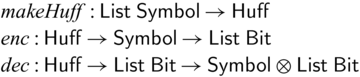
Here, ${{{{\mathit{enc}}}}}$
and
${{{{\mathit{enc}}}}}$
and ${{{{\mathit{dec}}}}}$
satisfy the properties
${{{{\mathit{dec}}}}}$
satisfy the properties ${dec} ~ h ~ ({enc} ~ h ~ {s} \mathbin{+\!+} {ys}) = (s, {ys})$
and
${dec} ~ h ~ ({enc} ~ h ~ {s} \mathbin{+\!+} {ys}) = (s, {ys})$
and ${dec} ~ h ~ {{ys}} = (s, {ys}')$
implies
${dec} ~ h ~ {{ys}} = (s, {ys}')$
implies ${enc} ~ {s} \mathbin{+\!+} {ys} = {ys}'$
, where
${enc} ~ {s} \mathbin{+\!+} {ys} = {ys}'$
, where $\mathbin{+\!+}$
is the list append function.
$\mathbin{+\!+}$
is the list append function.
Then, by enc and dec, we can define an bijective version encR as below.
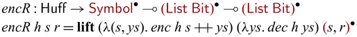
An encoder can be defined by first constructing a Huffman coding table and then encoding symbol by symbol. We can program this procedure in a natural way in Sparcl (Figure 6) by using ${{{{\mathbf{pin}}}}}$
. This is an example where multiple
${{{{\mathbf{pin}}}}}$
. This is an example where multiple ${{{{\mathbf{pin}}}}}$
s are used to convert data. The input symbol list is first passed to makeHuff under new to create a Huffman table h in the first
${{{{\mathbf{pin}}}}}$
s are used to convert data. The input symbol list is first passed to makeHuff under new to create a Huffman table h in the first ${{{{\mathbf{pin}}}}}$
; here the input symbol list is unidirectional (static), while the constructed Huffman table is invertible. Then, the input symbol list is encoded with the constructed Huffman table in the second
${{{{\mathbf{pin}}}}}$
; here the input symbol list is unidirectional (static), while the constructed Huffman table is invertible. Then, the input symbol list is encoded with the constructed Huffman table in the second ${{{{\mathbf{pin}}}}}$
; here the input symbol list is invertible, while the Huffman table is unidirectional (static). A subtlety here is the use of
${{{{\mathbf{pin}}}}}$
; here the input symbol list is invertible, while the Huffman table is unidirectional (static). A subtlety here is the use of ${eqHuff} : {\mathsf{Huff}} \to {\mathsf{Huff}} \to \mathsf{Bool}$
to test the equality of the Huffman encoding tables. This check ensures the property that
${eqHuff} : {\mathsf{Huff}} \to {\mathsf{Huff}} \to \mathsf{Bool}$
to test the equality of the Huffman encoding tables. This check ensures the property that ${{{{\mathbf{fwd}}}}} ~ {{huffCompress}} ~ ({{{{\mathbf{bwd}}}}} ~ {{huffCompress}} ~ (h, {ys})) = (h, {ys})$
. This equation holds only when h is the table obtained by applying makeHuff to the decoded text; indeed, eqHuff checks the condition. One could avoid this check by using the following unsafeNew instead.
${{{{\mathbf{fwd}}}}} ~ {{huffCompress}} ~ ({{{{\mathbf{bwd}}}}} ~ {{huffCompress}} ~ (h, {ys})) = (h, {ys})$
. This equation holds only when h is the table obtained by applying makeHuff to the decoded text; indeed, eqHuff checks the condition. One could avoid this check by using the following unsafeNew instead.
Two-pass Huffman coding in Sparcl.

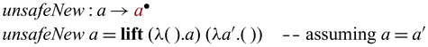
The use of ${unsafeNew} ~ a$
is safe only when its backward execution always receives a. Replacing new with unsafeNew violates this assumption, but for this case, the replacement just widens the domain of
${unsafeNew} ~ a$
is safe only when its backward execution always receives a. Replacing new with unsafeNew violates this assumption, but for this case, the replacement just widens the domain of ${{{{\mathbf{bwd}}}}} ~ {{huffCompress}}$
, which is acceptable even though
${{{{\mathbf{bwd}}}}} ~ {{huffCompress}}$
, which is acceptable even though ${{{{\mathbf{fwd}}}}} ~ {{huffCompress}}$
and
${{{{\mathbf{fwd}}}}} ~ {{huffCompress}}$
and ${{{{\mathbf{bwd}}}}} ~ {{huffCompress}}$
do not form a bijection due to unsafeNew. But in general this outcome is unreliable, unless the condition above can be guaranteed.
${{{{\mathbf{bwd}}}}} ~ {{huffCompress}}$
do not form a bijection due to unsafeNew. But in general this outcome is unreliable, unless the condition above can be guaranteed.
5.2.2 Concrete representation of Huffman tree in Sparcl
In the above we have modeled the case where different data structures are used for encoding and decoding, which demands the use of abstract type and consequently the use of ${{{{\mathbf{lift}}}}}$
ing. In this section, we define encR directly in Sparcl, which is possible when the same data structure is used for encoding and decoding.
${{{{\mathbf{lift}}}}}$
ing. In this section, we define encR directly in Sparcl, which is possible when the same data structure is used for encoding and decoding.
To do so, we first give a concrete representation of $\mathsf{Huff}$
.
$\mathsf{Huff}$
.
Here, $\mathsf{Lf} ~ s$
encodes s into the empty sequence, and
$\mathsf{Lf} ~ s$
encodes s into the empty sequence, and $\mathsf{Br} ~ l ~ r$
encodes s into
$\mathsf{Br} ~ l ~ r$
encodes s into $\mathsf{Cons} ~ {0} ~ c$
if l encodes s to c, and
$\mathsf{Cons} ~ {0} ~ c$
if l encodes s to c, and $\mathsf{Cons} ~ {1} ~ c$
if r encodes s to c. For example,
$\mathsf{Cons} ~ {1} ~ c$
if r encodes s to c. For example, $\mathsf{Br} ~ (\mathsf{Lf} ~ '{{{{\texttt{a}}}}}') ~ (\mathsf{Br} ~ (\mathsf{Lf} ~ '{{{{\texttt{b}}}}}') ~ (\mathsf{Br} ~ (\mathsf{Lf} ~ '{{{{\texttt{c}}}}}') ~ (\mathsf{Lf} ~ '{{{{\texttt{d}}}}}')))$
is the Huffman tree used to encode the example presented in the beginning of Section 5.2.
$\mathsf{Br} ~ (\mathsf{Lf} ~ '{{{{\texttt{a}}}}}') ~ (\mathsf{Br} ~ (\mathsf{Lf} ~ '{{{{\texttt{b}}}}}') ~ (\mathsf{Br} ~ (\mathsf{Lf} ~ '{{{{\texttt{c}}}}}') ~ (\mathsf{Lf} ~ '{{{{\texttt{d}}}}}')))$
is the Huffman tree used to encode the example presented in the beginning of Section 5.2.
Now let us define encR to be used in encode above. It is easier to define it via its inverse decR.
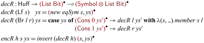
Here, ${member} : {\mathsf{Symbol}} \to {\mathsf{Huff}} \to \mathsf{Bool}$
is a membership test function. Recall that invert implements inversion of a bijection (Section 2). One can find that searching s in l for every recursive call is inefficient, and this cost can be avoided by additional information on
${member} : {\mathsf{Symbol}} \to {\mathsf{Huff}} \to \mathsf{Bool}$
is a membership test function. Recall that invert implements inversion of a bijection (Section 2). One can find that searching s in l for every recursive call is inefficient, and this cost can be avoided by additional information on $\mathsf{Br}$
that makes a Huffman tree a search tree. Another solution is to use different data structures for encoding and decoding as we demonstrated in Section 5.2.1.
$\mathsf{Br}$
that makes a Huffman tree a search tree. Another solution is to use different data structures for encoding and decoding as we demonstrated in Section 5.2.1.
5.2.3 Adaptive Huffman coding
In the above huffCompress, a Huffman coding table is fixed during compression which requires the preprocessing makeHuff to compute the table. This is sometimes suboptimal: for example, a one-pass method is preferred for streaming while a text could consist of several parts with very different frequency distributions of symbols.
Being adaptive means that we have the following two functions instead of makeHuff.
Instead of constructing a Huffman coding table beforehand, the Huffman coding table is constructed and changed throughout compression here.
The updating process of the Huffman coding table is the same in both compression and decompression, which means that Sparcl is effective for writing an invertible and adaptive version of Huffman coding in a natural way (Figure 7). This is another demonstration of the Sparcl’s strength in partial invertibility. Programming the same bijection in a fully invertible language gets a lot more complicated due to the irreversible nature of updHuff.
Adaptive Huffman coding in Sparcl.

5.3 Arithmetic coding
The idea of arithmetic coding is to encode the entire message into a single number in the range [0,1). It achieves this by assigning a range to each symbol and encode the symbol sequence by narrowing the ranges. For example, suppose that symbols ${{{{\texttt{a}}}}}$
,
${{{{\texttt{a}}}}}$
, ${{{{\texttt{b}}}}}$
,
${{{{\texttt{b}}}}}$
, ${{{{\texttt{c}}}}}$
, and
${{{{\texttt{c}}}}}$
, and ${{{{\texttt{d}}}}}$
are assigned with ranges
${{{{\texttt{d}}}}}$
are assigned with ranges $[0, 0.6)$
,
$[0, 0.6)$
, $[0.6, 0.8)$
,
$[0.6, 0.8)$
, $[0.8, 0.9)$
, and
$[0.8, 0.9)$
, and $[0.9, 1.0)$
. The compression algorithm retains a range [l, r), narrows the range to
$[0.9, 1.0)$
. The compression algorithm retains a range [l, r), narrows the range to $[l + (r - l) l_s, l + (r - l) r_s)$
when it reads a symbol s to which
$[l + (r - l) l_s, l + (r - l) r_s)$
when it reads a symbol s to which $[l_s,r_s)$
is associated, and finally yields a real in [l,r). For example, reading a text
$[l_s,r_s)$
is associated, and finally yields a real in [l,r). For example, reading a text ${{{{\texttt{aabacabdaa}}}}}$
, the range is narrowed into
${{{{\texttt{aabacabdaa}}}}}$
, the range is narrowed into $[0.25258176, 0.2526004224)$
and a real
$[0.25258176, 0.2526004224)$
and a real $0.010000001010101$
(in base 2) can be picked. Since the first and last bits are redundant, the number can be represented by a 14-bit code
$0.010000001010101$
(in base 2) can be picked. Since the first and last bits are redundant, the number can be represented by a 14-bit code ${{{{\texttt{01000000101010}}}}}$
, which is smaller than the 20 bit code produced by the naive encoding. Notice that the code
${{{{\texttt{01000000101010}}}}}$
, which is smaller than the 20 bit code produced by the naive encoding. Notice that the code ${{{{\texttt{0}}}}}$
corresponds to multiple texts
${{{{\texttt{0}}}}}$
corresponds to multiple texts ${{{{\texttt{a}}}}}$
,
${{{{\texttt{a}}}}}$
, ${{{{\texttt{aa}}}}}$
,
${{{{\texttt{aa}}}}}$
, ${{{{\texttt{aaa}}}}}, \dots$
. There are several ways to avoid this ambiguity in decoding; here we assume a special end-of-stream symbol
${{{{\texttt{aaa}}}}}, \dots$
. There are several ways to avoid this ambiguity in decoding; here we assume a special end-of-stream symbol $\mathsf{EOS}$
whose range does not appear in the symbol range list.
$\mathsf{EOS}$
whose range does not appear in the symbol range list.
As a simplification, we only consider ranges defined by rational numbers $\mathbb{Q}$
. Specifically, we assume the following type and functions.
$\mathbb{Q}$
. Specifically, we assume the following type and functions.
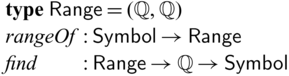
Here, rangeOf returns a range assigned to a given symbol, and find takes a range and a rational in the range, and returns a symbol of which the subdivision of the range contains the rational. In addition, we will use the following functions.
The narrowing of ranges can be implemented straightforwardly as below.
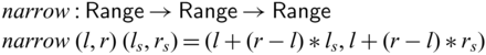
In what follows, narrow is used only with rangeOf. So, we define the following function for convenience.
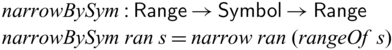
These functions satisfy the following property.
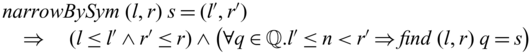
Although $\lambda {s}. {narrow} ~ {(l,r)} ~ {({rangeOf} ~ {s})}$
is an injection (provided that
$\lambda {s}. {narrow} ~ {(l,r)} ~ {({rangeOf} ~ {s})}$
is an injection (provided that $r - l > 0$
), the arithmetic coding does not use the property in decompression because in decompression the result is a rational number instead of a range.
$r - l > 0$
), the arithmetic coding does not use the property in decompression because in decompression the result is a rational number instead of a range.
As the first step, we define a unidirectional version that return a rational instead of a bit sequence for simplicity.
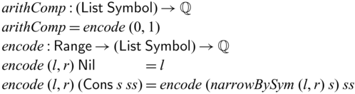
We can see from the definition that unidirectional and invertible computation is mixed together. On one hand, the second component of the range is nonlinear (discarded when encode meats $\mathsf{Nil}$
), meaning that the range must be treated as unidirectional. On the other hand, a rational in the range (here we just use the lower bound for simplicity) goes to the final result of arithComp, which means that the range should be treated as invertible. The
$\mathsf{Nil}$
), meaning that the range must be treated as unidirectional. On the other hand, a rational in the range (here we just use the lower bound for simplicity) goes to the final result of arithComp, which means that the range should be treated as invertible. The ${{{{\mathbf{pin}}}}}$
operator could be a solution to the issue. Since we want to use the unidirectional function narrowBySym, it is natural to
${{{{\mathbf{pin}}}}}$
operator could be a solution to the issue. Since we want to use the unidirectional function narrowBySym, it is natural to ${{{{\mathbf{pin}}}}}$
the symbol s to narrow the range, which belongs to the unidirectional world. However, there is a problem. Using
${{{{\mathbf{pin}}}}}$
the symbol s to narrow the range, which belongs to the unidirectional world. However, there is a problem. Using ${{{{\mathbf{pin}}}}}$
produces an invertible product
${{{{\mathbf{pin}}}}}$
produces an invertible product ![]() with the symbol remaining in the output. In Huffman coding as we have seen, this is not a problem because the two component are combined as the final product. But here the information of
with the symbol remaining in the output. In Huffman coding as we have seen, this is not a problem because the two component are combined as the final product. But here the information of $\mathsf{Symbol}$
is redundant as it is already retained by the rational in the second component. We need a way to reveal this redundancy and safely discard the symbol.
$\mathsf{Symbol}$
is redundant as it is already retained by the rational in the second component. We need a way to reveal this redundancy and safely discard the symbol.
The solution lies with the delete function in Section 5.1.3. For this particular case of the arithmetic coding, the following derived version is more convenient.
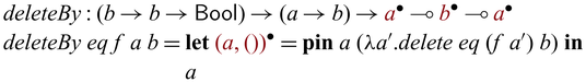
By using deleteBy with find (part of the arithmetic encoding API), we can write an invertible version as below.
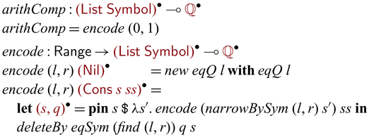
Here, eqQ and eqSym are equivalence tests on $\mathbb{Q}$
and
$\mathbb{Q}$
and $\mathsf{Symbol}$
, respectively. The operator
$\mathsf{Symbol}$
, respectively. The operator $({{{{\mathbin{\texttt{\$}}}}}})$
, defined by
$({{{{\mathbin{\texttt{\$}}}}}})$
, defined by $({{{{\mathbin{\texttt{\$}}}}}}) = \lambda f. \lambda x.f ~ x$
, is used to avoid parentheses, which is right-associative and has the lowest precedence unlike function application. The with-condition
$({{{{\mathbin{\texttt{\$}}}}}}) = \lambda f. \lambda x.f ~ x$
, is used to avoid parentheses, which is right-associative and has the lowest precedence unlike function application. The with-condition ${enQ} ~ l$
becomes false for any result from the second branch of encode; the assumption on
${enQ} ~ l$
becomes false for any result from the second branch of encode; the assumption on $\mathsf{EOS}$
guarantees that encode eventually meats
$\mathsf{EOS}$
guarantees that encode eventually meats $\mathsf{EOS}$
and changes the lower bound of the range. It is worth noting that, in this case, the check eqSym involved in deleteBy always succeeds thanks to the property about narrowBySym and find above. Thus, we can use the “unsafe” variants of delete and deleteBy safely here. Also, for this particular case, we can replace new with unsafeNew, if we admit some unsafety: this replacement just makes
$\mathsf{EOS}$
and changes the lower bound of the range. It is worth noting that, in this case, the check eqSym involved in deleteBy always succeeds thanks to the property about narrowBySym and find above. Thus, we can use the “unsafe” variants of delete and deleteBy safely here. Also, for this particular case, we can replace new with unsafeNew, if we admit some unsafety: this replacement just makes ${{{{\mathbf{bwd}}}}} ~ {{arithComp}}$
accept more inputs than what
${{{{\mathbf{bwd}}}}} ~ {{arithComp}}$
accept more inputs than what ${{{{\mathbf{fwd}}}}} ~ {{arithComp}}$
can return.
${{{{\mathbf{fwd}}}}} ~ {{arithComp}}$
can return.
As a general observation, programming in a compositional way in Sparcl is easier when a component function, after fixing some arguments, transforms all and only the information of the input to the output. In the Huffman coding example, where a bounded number of bits are transmitted for a symbol, both enR and encode satisfy this criterion; and as a result, its definition is mostly straightforward. In contrast, in arithmetic coding, even recursive calls of encode do not satisfy the criterion, as a single bit of an input could affect an unbounded number of positions in the output, which results in the additional programming effort as we demonstrated in the above.
5.4 LZ77 compression
LZ77 (Ziv & Lempel, Reference Ziv and Lempel1977) and its variant (such as LZ78 and LZSS) are also some of the most popular compression algorithms. The basic idea is to use a string of a fixed length (called a window) from the already traversed part of the message as a dictionary and repeatedly replace to be traversed strings with their entries (matching positions and lengths) in the dictionary. To do so, LZ77 maintains two buffers: the window and the look-ahead buffer (Salomon, Reference Salomon2008), where the window is searched for the matching position and length of the string in the look-ahead buffer. When the search succeeds, the algorithm emits the matching position and length and shifts both buffers by the matching length.Footnote
17
Otherwise, it emits the first character and shifts the two buffers by one. For example, when the window size is 4 and the look-ahead buffer size is 3, for an window ${{{{\texttt{d}}}}}{{{{\texttt{a}}}}}{{{{\texttt{b}}}}}{{{{\texttt{c}}}}}$
and an input string
${{{{\texttt{d}}}}}{{{{\texttt{a}}}}}{{{{\texttt{b}}}}}{{{{\texttt{c}}}}}$
and an input string ${{{{\texttt{abda}}}}}$
, the algorithm yields
${{{{\texttt{abda}}}}}$
, the algorithm yields $(3,2) {{{{\texttt{d}}}}}{{{{\texttt{a}}}}}$
, as below
$(3,2) {{{{\texttt{d}}}}}{{{{\texttt{a}}}}}$
, as below
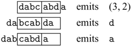
where (3,2) means that the string ${{{{\texttt{a}}}}}{{{{\texttt{b}}}}}$
of length 2 appears in the window at position 3 (counted from the last). In general, the end of a matched string may not be in the window but the look-ahead buffer. For example, for
${{{{\texttt{a}}}}}{{{{\texttt{b}}}}}$
of length 2 appears in the window at position 3 (counted from the last). In general, the end of a matched string may not be in the window but the look-ahead buffer. For example, for ![]() the algorithm emits (1,4).
the algorithm emits (1,4).
The basic idea of our implementation is to use ${{{{\mathbf{pin}}}}}$
to convert the input string from invertible to unidirectional to allow overlapping in searching. Hence, we prepare the following unidirectional functions for the manipulation of the window, which is an abstract type
${{{{\mathbf{pin}}}}}$
to convert the input string from invertible to unidirectional to allow overlapping in searching. Hence, we prepare the following unidirectional functions for the manipulation of the window, which is an abstract type $\mathsf{Window}$
.
$\mathsf{Window}$
.
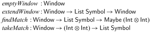
Here, the last two functions satisfy the following property.
Also, we use the following type for the output code.
We do not need to represent the look-ahead buffer explicitly, as it is hidden in the findMatch function. Instead of using custom-sized integers, we use $\mathsf{Int}$
to represent both matching positions (bounded by the size of the window) and matching lengths (bounded by the size of the look-ahead buffer) for simplicity.
$\mathsf{Int}$
to represent both matching positions (bounded by the size of the window) and matching lengths (bounded by the size of the look-ahead buffer) for simplicity.
Figure 8 shows an implementation of an invertible LZ77 compression in Sparcl. We omit the definition of ${eqMatchRes} : \mathsf{Maybe} ~ (\mathsf{Int} \otimes \mathsf{Int}) \to \mathsf{Maybe} ~ (\mathsf{Int} \otimes \mathsf{Int}) \to \mathsf{Bool}$
and
${eqMatchRes} : \mathsf{Maybe} ~ (\mathsf{Int} \otimes \mathsf{Int}) \to \mathsf{Maybe} ~ (\mathsf{Int} \otimes \mathsf{Int}) \to \mathsf{Bool}$
and ${eqStr} : \mathsf{List} ~ \mathsf{Symbol} \to \mathsf{List} ~ \mathsf{Symbol} \to \mathsf{Bool}$
. Similarly to the arithmetic coding example, we also use the new/delete trick here. The property above of findMatch and takeMatch ensures that the delete in encode must succeed in the forward evaluation, meaning that we can replace the delete by its unsafe variant similarly to the arithmetic coding example. It is also similar to the previous examples that the backward evaluation of lz77 can only accept the encoded string that the corresponding forward evaluation can produce. This is inconvenient in practice, because there in general are many compression algorithms that correspond to a decompression algorithm. Fortunately, the same solution to the previous examples also apply to this example: for this particular case, replacing new with unsafeNew is widen the domain of the backward execution, without risking the expected behavior that decompression after compression should yield the original data.
${eqStr} : \mathsf{List} ~ \mathsf{Symbol} \to \mathsf{List} ~ \mathsf{Symbol} \to \mathsf{Bool}$
. Similarly to the arithmetic coding example, we also use the new/delete trick here. The property above of findMatch and takeMatch ensures that the delete in encode must succeed in the forward evaluation, meaning that we can replace the delete by its unsafe variant similarly to the arithmetic coding example. It is also similar to the previous examples that the backward evaluation of lz77 can only accept the encoded string that the corresponding forward evaluation can produce. This is inconvenient in practice, because there in general are many compression algorithms that correspond to a decompression algorithm. Fortunately, the same solution to the previous examples also apply to this example: for this particular case, replacing new with unsafeNew is widen the domain of the backward execution, without risking the expected behavior that decompression after compression should yield the original data.
LZ77 in Sparcl.

6 Related work
6.1 Program inversion and invertible/reversible computation
In the literature of program inversion (a program transformation technique to find $f^{-1}$
for a given f), it is known that an inverse of a function may not arise from reversing all the execution steps of the original program. Partial inversion (Romanenko, Reference Romanenko1991; Nishida et al., 2005) addresses the problem by classifying inputs/outputs into known and unknown, where known information is available also for inverses. This classification can be viewed as a binding-time analysis (Gomard & Jones, Reference Gomard and Jones1991; Jones et al., Reference Jones, Gomard and Sestoft1993) where the known part is treated as static. The partial inversion is further extended so that the return values of inverses are treated as known as well (Almendros-Jiménez & Vidal, Reference Almendros-Jiménez and Vidal2006; Kirkeby & Glück, Reference Kirkeby and Glück2019, Reference Kirkeby and Glück2020); in this case, it can no longer be explained as a binding-time analysis. This extension introduces additional power, but makes inversion fragile as success depends on which function is inverted first. For example, the partial inversion for goSubs succeeds when it inverts
$f^{-1}$
for a given f), it is known that an inverse of a function may not arise from reversing all the execution steps of the original program. Partial inversion (Romanenko, Reference Romanenko1991; Nishida et al., 2005) addresses the problem by classifying inputs/outputs into known and unknown, where known information is available also for inverses. This classification can be viewed as a binding-time analysis (Gomard & Jones, Reference Gomard and Jones1991; Jones et al., Reference Jones, Gomard and Sestoft1993) where the known part is treated as static. The partial inversion is further extended so that the return values of inverses are treated as known as well (Almendros-Jiménez & Vidal, Reference Almendros-Jiménez and Vidal2006; Kirkeby & Glück, Reference Kirkeby and Glück2019, Reference Kirkeby and Glück2020); in this case, it can no longer be explained as a binding-time analysis. This extension introduces additional power, but makes inversion fragile as success depends on which function is inverted first. For example, the partial inversion for goSubs succeeds when it inverts $x- n$
first, but fails if it tried to invert
$x- n$
first, but fails if it tried to invert ${goSubs} ~ x ~ {xs}$
first. The design of Sparcl is inspired by these partial inversion methods: we use
${goSubs} ~ x ~ {xs}$
first. The design of Sparcl is inspired by these partial inversion methods: we use ![]() -types to distinguish the known and unknown parts, and
-types to distinguish the known and unknown parts, and ${{{{\mathbf{pin}}}}}$
together with
${{{{\mathbf{pin}}}}}$
together with ${{{{\mathbf{case}}}}}$
to control orders. Semi inversion (Mogensen, Reference Mogensen2005) essentially converts a program to logic programs and then tries to convert it back to a functional inverse program, which also allows the original and inverse programs to have common computations. Its extension (Mogensen, Reference Mogensen2008) can handle a limited form of function arguments. Specifically, such function arguments must be names of top-level functions; neither closures nor partial applications is supported. The Inversion Framework (Kirkeby & Glück, Reference Kirkeby and Glück2020) unifies the partial and semi inversion methods based on the authors’ reformulation (Kirkeby & Glück, Reference Kirkeby and Glück2019) of semi inversion for conditional constructor term rewriting systems (Terese, 2003). The PINS system allows users to specify control structures as they sometimes differ from the original program (Srivastava et al.,Reference Srivastava, Gulwani, Chaudhuri and Foster2011). As we mentioned in Section 1, these program inversion methods may fail, and often for reasons that are not obvious to programmers.
${{{{\mathbf{case}}}}}$
to control orders. Semi inversion (Mogensen, Reference Mogensen2005) essentially converts a program to logic programs and then tries to convert it back to a functional inverse program, which also allows the original and inverse programs to have common computations. Its extension (Mogensen, Reference Mogensen2008) can handle a limited form of function arguments. Specifically, such function arguments must be names of top-level functions; neither closures nor partial applications is supported. The Inversion Framework (Kirkeby & Glück, Reference Kirkeby and Glück2020) unifies the partial and semi inversion methods based on the authors’ reformulation (Kirkeby & Glück, Reference Kirkeby and Glück2019) of semi inversion for conditional constructor term rewriting systems (Terese, 2003). The PINS system allows users to specify control structures as they sometimes differ from the original program (Srivastava et al.,Reference Srivastava, Gulwani, Chaudhuri and Foster2011). As we mentioned in Section 1, these program inversion methods may fail, and often for reasons that are not obvious to programmers.
Embedded languages can be seen as two-staged (a host and a guest), and there are several embedded invertible/reversible programming languages. A popular approach to implement such languages is based on combinators (Reference Mu, Hu and TakeichiMu et al., 2004b
; Rendel & Ostermann, Reference Rendel and Ostermann2010; Kennedy & Vytiniotis, Reference Kennedy and Vytiniotis2012; Wang et al., Reference Wang, Gibbons, Matsuda and Hu2013), in which users program by composing bijections through designated combinators. To the best of our knowledge, only (Kennedy& Vytiniotis, Reference Kennedy and Vytiniotis2012) has an operator like ![]() , which is key to partial invertibility. More specifically, (Kennedy& Vytiniotis, Reference Kennedy and Vytiniotis2012) has an operator
, which is key to partial invertibility. More specifically, (Kennedy& Vytiniotis, Reference Kennedy and Vytiniotis2012) has an operator ${depGame} :: \mathsf{Game} ~ a \to (a \to \mathsf{Game} ~ b) \to \mathsf{Game} ~ (a,b)$
. The types suggest that
${depGame} :: \mathsf{Game} ~ a \to (a \to \mathsf{Game} ~ b) \to \mathsf{Game} ~ (a,b)$
. The types suggest that $\mathsf{Game}$
and
$\mathsf{Game}$
and ![]() play a similar role; indeed they both represent invertibility but in different ways. In their system,
play a similar role; indeed they both represent invertibility but in different ways. In their system, $\mathsf{Game} ~ a$
represents (total) bijections from bit sequences and a-typed values, while in our system
$\mathsf{Game} ~ a$
represents (total) bijections from bit sequences and a-typed values, while in our system ![]() represents a bijection whose range is A but domain is determined when
represents a bijection whose range is A but domain is determined when ${{{{\mathbf{unlift}}}}}$
is applied. One consequence of this difference is that, in their domain-specific system, there is no restriction of using a value
${{{{\mathbf{unlift}}}}}$
is applied. One consequence of this difference is that, in their domain-specific system, there is no restriction of using a value $v :: \mathsf{Game} ~ a$
linearly, because there is no problem of using an encoder/decoder pair for type a multiple times, even though nonlinear use of
$v :: \mathsf{Game} ~ a$
linearly, because there is no problem of using an encoder/decoder pair for type a multiple times, even though nonlinear use of ![]() , especially discarding, leads to non-bijectivity. Another consequence of the difference is that their system is hardwired to bit sequences and therefore does not support deriving general bijections between a and b from
, especially discarding, leads to non-bijectivity. Another consequence of the difference is that their system is hardwired to bit sequences and therefore does not support deriving general bijections between a and b from $\mathsf{Game} ~ a \to \mathsf{Game} ~ b$
, whereas we can obtain a (not-necessarily-total) bijections between A and B from any function of type
$\mathsf{Game} ~ a \to \mathsf{Game} ~ b$
, whereas we can obtain a (not-necessarily-total) bijections between A and B from any function of type ![]() that does not contain linear free variables.
that does not contain linear free variables.
The ${{{{\mathbf{pin}}}}}$
operator can be seen as a functional generalization of reversible update statements (Axelsen et al., Reference Axelsen, Glück and Yokoyama2007)
${{{{\mathbf{pin}}}}}$
operator can be seen as a functional generalization of reversible update statements (Axelsen et al., Reference Axelsen, Glück and Yokoyama2007) $x \mathbin{{{\oplus}{=}}} e$
in reversible imperative languages (Lutz, Reference Lutz1986; Frank, Reference Frank1997; Yokoyama et al., Reference Yokoyama, Axelsen and Glück2008; Glück & Yokoyama, Reference Glück and Yokoyama2016), of which the inverse is given by
$x \mathbin{{{\oplus}{=}}} e$
in reversible imperative languages (Lutz, Reference Lutz1986; Frank, Reference Frank1997; Yokoyama et al., Reference Yokoyama, Axelsen and Glück2008; Glück & Yokoyama, Reference Glück and Yokoyama2016), of which the inverse is given by $x\mathbin{{{\ominus}{=}}} e$
with
$x\mathbin{{{\ominus}{=}}} e$
with $\ominus$
satisfying
$\ominus$
satisfying $(x \oplus y) \ominus y = x$
for any y; examples of
$(x \oplus y) \ominus y = x$
for any y; examples of $\oplus$
(and
$\oplus$
(and $\ominus$
) include addition, subtraction, bitwise XOR, and replacement of nil (Glück & Yokoyama, Reference Glück and Yokoyama2016) as a form of reversible copying (Glück and Kawabe, Reference Glück and Kawabe2003). Having
$\ominus$
) include addition, subtraction, bitwise XOR, and replacement of nil (Glück & Yokoyama, Reference Glück and Yokoyama2016) as a form of reversible copying (Glück and Kawabe, Reference Glück and Kawabe2003). Having $(x \oplus y) \ominus y$
means that
$(x \oplus y) \ominus y$
means that $\oplus$
and
$\oplus$
and $\ominus$
are partially invertible, and indicates that they correspond to the second argument of
$\ominus$
are partially invertible, and indicates that they correspond to the second argument of ${{{{\mathbf{pin}}}}}$
. Whereas the operators such as
${{{{\mathbf{pin}}}}}$
. Whereas the operators such as $\oplus$
and
$\oplus$
and $\ominus$
are fixed in those languages, in Sparcl, leveraging its higher-orderness, any function of an appropriate type can be used as the second argument of
$\ominus$
are fixed in those languages, in Sparcl, leveraging its higher-orderness, any function of an appropriate type can be used as the second argument of ${{{{\mathbf{pin}}}}}$
, which leads to concise function definitions as demonstrated in goSub in Section 2 and the examples in Section 5.
${{{{\mathbf{pin}}}}}$
, which leads to concise function definitions as demonstrated in goSub in Section 2 and the examples in Section 5.
Most of the existing reversible programming languages (Lutz, Reference Lutz1986; Baker, Reference Baker1992; Frank, Reference Frank1997; Reference Mu, Hu and TakeichiMu et al., 2004b
; Yokoyama et al., Reference Yokoyama, Axelsen and Glück2008, Reference Yokoyama, Axelsen and Glück2011; Wang et al., Reference Wang, Gibbons, Matsuda and Hu2013) do not support function values, and higher-order reversible programming languages are uncommon. One notable exception is Abramsky (Reference Abramsky2005) that shows a subset of the linear $\lambda$
-calculus concerning
$\lambda$
-calculus concerning $\multimap$
and
$\multimap$
and ${!}$
(more precisely, a combinator logic that corresponds to the subset) can be interpreted as manipulations of (not-necessarily-total) bijections. However, it is known to be difficult to extend their system to primitives such as constructors and invertible pattern matching (Abramsky, Reference Abramsky2005, Section 7). Abramsky (Reference Abramsky2005)’s idea is based on the fact that a certain linear calculus is interpreted in a compact closed category, which has a dual object
${!}$
(more precisely, a combinator logic that corresponds to the subset) can be interpreted as manipulations of (not-necessarily-total) bijections. However, it is known to be difficult to extend their system to primitives such as constructors and invertible pattern matching (Abramsky, Reference Abramsky2005, Section 7). Abramsky (Reference Abramsky2005)’s idea is based on the fact that a certain linear calculus is interpreted in a compact closed category, which has a dual object $A^{*}$
such that
$A^{*}$
such that $A^{*} \otimes B$
serves as a function (i.e., internal hom) object, and that we can construct (Joyal et al., Reference Joyal, Street and Verity1996) a compact closed category from the category of not-necessary-total bijections (Abramsky et al., Reference Abramsky, Haghverdi and Scott2002). Recently, Chen & Sabry (Reference Chen and Sabry2021) designed a language that has fractional and negative types inspired by compact closed categories. In the language, a negative type
$A^{*} \otimes B$
serves as a function (i.e., internal hom) object, and that we can construct (Joyal et al., Reference Joyal, Street and Verity1996) a compact closed category from the category of not-necessary-total bijections (Abramsky et al., Reference Abramsky, Haghverdi and Scott2002). Recently, Chen & Sabry (Reference Chen and Sabry2021) designed a language that has fractional and negative types inspired by compact closed categories. In the language, a negative type $-A$
is a dual of A for
$-A$
is a dual of A for $\oplus$
, and constitutes a “function” type
$\oplus$
, and constitutes a “function” type $-A \oplus B$
that satisfies the isomorphism
$-A \oplus B$
that satisfies the isomorphism $A \oplus B \leftrightarrow C \simeq A \leftrightarrow -B \oplus C$
, where
$A \oplus B \leftrightarrow C \simeq A \leftrightarrow -B \oplus C$
, where $\leftrightarrow$
denotes bijections. One of the applications of the negative type is to define a loop like operation called the trace operator, which has a similar behavior to trace in Section 3.6.4. The fractional types in the language are indexed by values as
$\leftrightarrow$
denotes bijections. One of the applications of the negative type is to define a loop like operation called the trace operator, which has a similar behavior to trace in Section 3.6.4. The fractional types in the language are indexed by values as $1/(v : A)$
, which represents the obligation to erase an ancilla value v, and hence the corresponding application form does perform the erasure. However, behavior of both
$1/(v : A)$
, which represents the obligation to erase an ancilla value v, and hence the corresponding application form does perform the erasure. However, behavior of both $-A \oplus B$
and
$-A \oplus B$
and $1/(v : A) \otimes B$
is different from what we expect for functions: the former operates on
$1/(v : A) \otimes B$
is different from what we expect for functions: the former operates on $\oplus$
instead of
$\oplus$
instead of $\otimes$
, and the latter only accepts the input v.
$\otimes$
, and the latter only accepts the input v.
A few reversible functional programming languages also support a limited form of partial invertibility. RFunT,Footnote
18
a typed variant of RFun (Yokoyama et al. Reference Yokoyama, Axelsen and Glück2011)with Haskell-like syntax, allows a function to take additional parameters called ancilla parameters. The reversibility restriction is relaxed for ancilla parameters, and they can be discarded and pattern-matched without requiring a way to determine branching from their results. However, these ancilla parameters are supposed to be translated into auxiliary inputs and outputs that stay the same before and after reversible computation, and mixing unidirectional computation is not their primary purpose. In fact, very limited operations are allowed for these ancilla data by the system. CoreFun also supports ancilla parameters (Jacobsen et al. Reference Jacobsen, Kaarsgaard and Thomsen2018). Their ancilla parameters are treated as static inputs to reversible functions, and arguments that appear at ancilla positions are free from the linearity restriction.Footnote
19
The system is overly conservative: all the functions are (partially) reversible, and thus functions themselves used in the ancilla positions must obey the linearity restriction. (Jeopardy Reference Kristensen, Kaarsgaard and ThomsenKristensen et al., 2022b
)Footnote
20
is a work-in-progress reversible language, which plans to support partial invertibility via program analysis. The implicit argument analysis (Reference Kristensen, Kaarsgaard and ThomsenKristensen et al., 2022a
), which Jeopardy uses, identifies which arguments are available (or, known (Nishida et al., Reference Nishida, Sakai and Sakabe2005)) for each functional call and for the forward/backward execution. However, the inverse execution based on the analysis has neither been formalized nor implemented to the best of the authors’ knowledge. More crucially, RFunT, CoreFun and Jeopardy are first-order languages (to be precise, they allow top-level function names to be used as values, but not partial application or $\lambda$
-abstraction), which limits flexible programming. In contrast,
$\lambda$
-abstraction), which limits flexible programming. In contrast, ![]() is an ordinary type in Sparcl, and there is no syntactic restriction on expressions of type
is an ordinary type in Sparcl, and there is no syntactic restriction on expressions of type ![]() . This feature, combined with the higher-orderness, gives extra flexibility in mixing unidirectional and invertible programming. For example, Sparcl allows a function composition operator that can be used for both unidirectional (hence unrestricted) and invertible (hence linear) functions, using multiplicity polymorphism (Bernardy et al., Reference Bernardy, Boespflug, Newton, Peyton Jones and Spiwack2018; Matsuda, Reference Matsuda2020).
. This feature, combined with the higher-orderness, gives extra flexibility in mixing unidirectional and invertible programming. For example, Sparcl allows a function composition operator that can be used for both unidirectional (hence unrestricted) and invertible (hence linear) functions, using multiplicity polymorphism (Bernardy et al., Reference Bernardy, Boespflug, Newton, Peyton Jones and Spiwack2018; Matsuda, Reference Matsuda2020).
6.2 Functional quantum programming languages
In quantum programming, many operation are reversible, and there are a few higher-order quantum programming languages (Selinger & Valiron, Reference Selinger and Valiron2006; Rios & Selinger, Reference Rios and Selinger2017). Among them, the type system of Proto-Quipper-M (Rios & Selinger, Reference Rios and Selinger2017) is similar to ${{{{\lambda^{\mathrm{PI}}_{\to}}}}}$
in the sense that it also uses a linear-type system and distinguishes two sorts of variable environments as we do with
${{{{\lambda^{\mathrm{PI}}_{\to}}}}}$
in the sense that it also uses a linear-type system and distinguishes two sorts of variable environments as we do with $\Gamma$
and
$\Gamma$
and $\Theta$
, although the semantic back-ends are different. They do not have any language construct that introduces new variables to the second sort of environments (a counterpart of our
$\Theta$
, although the semantic back-ends are different. They do not have any language construct that introduces new variables to the second sort of environments (a counterpart of our $\Theta$
), because their language does not have a counterpart to our invertible
$\Theta$
), because their language does not have a counterpart to our invertible ${{{{\mathbf{case}}}}}$
.
${{{{\mathbf{case}}}}}$
.
It is also interesting to see that some quantum languages allow weakening (i.e., discarding) (Selinger & Valiron, Reference Selinger and Valiron2006) and some allow contraction (i.e., copying) (Altenkirch & Grattage, Reference Altenkirch and Grattage2005). In these frameworks, weakening is allowed because one can throw away a quantum bit after measuring, and contraction is allowed because states can be shared through introducing entanglements. As our goal is to obtain a bijection as final product, weakening in general is not possible in our context. On the other hand, it is a design choice whether or not contraction is allowed. Since the inverse of copying can be given by equivalence checking and vice versa (Glück and Kawabe, Reference Glück and Kawabe2003). However, careless uses of copying may result in unintended domain restriction. Moreover supporting such a feature requires hard-wired equivalence checks for all types of variables that can be in $\Theta$
(notice that multiple uses of a variable in
$\Theta$
(notice that multiple uses of a variable in $\Gamma$
will be reduced to multiple uses of variables in
$\Gamma$
will be reduced to multiple uses of variables in $\Theta$
(Matsuda & Wang, Reference Matsuda and Wang2018c).). This requires the type system to distinguish types that can be in
$\Theta$
(Matsuda & Wang, Reference Matsuda and Wang2018c).). This requires the type system to distinguish types that can be in $\Theta$
from general ones, as types such as
$\Theta$
from general ones, as types such as $A \multimap B$
do not have decidable equality. Moreover, the hard-wired equivalence checks would prevent users from using abstract types such as
$A \multimap B$
do not have decidable equality. Moreover, the hard-wired equivalence checks would prevent users from using abstract types such as $\mathsf{Huff}$
in Section 5, for which the definition of equivalence can differ from that on their concrete representations.
$\mathsf{Huff}$
in Section 5, for which the definition of equivalence can differ from that on their concrete representations.
6.3 Bidirectional programming languages
It is perhaps not surprising that many of the concerns in designing invertible/bijective/reversible languages are shared by the closely related field of bidirectional programming (Foster et al.,Reference Foster, Greenwald, Moore, Pierce and Schmitt2007). A bidirectional transformation is a generalization of a pair of inverses that allows a component to be non-bijective; for example, an (asymmetric) bidirectional transformation between a and b are given by two functions called ${get} : a \to b$
and
${get} : a \to b$
and ${put} : a \to b \to a$
(Foster et al.,Reference Foster, Greenwald, Moore, Pierce and Schmitt2007). Similarly to ours, in the bidirectional language HOBiT (Matsuda & Wang, Reference Matsuda and Wang2018c)., a bidirectional transformation between a and b is represented by a function from
${put} : a \to b \to a$
(Foster et al.,Reference Foster, Greenwald, Moore, Pierce and Schmitt2007). Similarly to ours, in the bidirectional language HOBiT (Matsuda & Wang, Reference Matsuda and Wang2018c)., a bidirectional transformation between a and b is represented by a function from $\mathbf{B} ~ a$
to
$\mathbf{B} ~ a$
to $\mathbf{B} ~ b$
, and top-level functions of type
$\mathbf{B} ~ b$
, and top-level functions of type $\mathbf{B} ~ a \to \mathbf{B} ~ b$
can be converted to a bidirectional transformation between a and b. Despite the similarity, there are unique challenges in invertible programming: notably, the handling of partial invertibility that this paper focuses on and the introduction of the operator
$\mathbf{B} ~ a \to \mathbf{B} ~ b$
can be converted to a bidirectional transformation between a and b. Despite the similarity, there are unique challenges in invertible programming: notably, the handling of partial invertibility that this paper focuses on and the introduction of the operator ${{{{\mathbf{pin}}}}}$
as a solution. Another difference is that Sparcl is based on a linear type system, which, as we have seen, perfectly supports the need for the intricate connections between unidirectional and inverse computation in addressing partial invertibility. One of the consequences of this difference in the underlying type system is that (Matsuda & Wang, Reference Matsuda and Wang2018c). can only interpret top-level functions of type
${{{{\mathbf{pin}}}}}$
as a solution. Another difference is that Sparcl is based on a linear type system, which, as we have seen, perfectly supports the need for the intricate connections between unidirectional and inverse computation in addressing partial invertibility. One of the consequences of this difference in the underlying type system is that (Matsuda & Wang, Reference Matsuda and Wang2018c). can only interpret top-level functions of type $\mathbf{B} ~ a \to \mathbf{B} ~ b$
as bidirectional transformations between a and b, yet we can interpret functions of type
$\mathbf{B} ~ a \to \mathbf{B} ~ b$
as bidirectional transformations between a and b, yet we can interpret functions of type ![]() in any places as bijections between A and B, as long as they have no linear free variables. Linear types also clarify the roles of values and prevent users from unintended failures caused by erroneous use of variables. For example, the type
in any places as bijections between A and B, as long as they have no linear free variables. Linear types also clarify the roles of values and prevent users from unintended failures caused by erroneous use of variables. For example, the type ![]() of
of ${{{{\mathbf{pin}}}}}$
clarifies that the function argument of
${{{{\mathbf{pin}}}}}$
clarifies that the function argument of ${{{{\mathbf{pin}}}}}$
can safely discard or copy its input as the nonlinear uses do not affect the domain of the resulting bijection. It is worth mentioning that, in addition to bidirectional transformations, HOBiT provides a way to lift bidirectional combinators (i.e., functions that take and return bidirectional transformations). However, the same is not obvious in Sparcl due to its linear type system, as the combinators need to take care of the manipulation of
${{{{\mathbf{pin}}}}}$
can safely discard or copy its input as the nonlinear uses do not affect the domain of the resulting bijection. It is worth mentioning that, in addition to bidirectional transformations, HOBiT provides a way to lift bidirectional combinators (i.e., functions that take and return bidirectional transformations). However, the same is not obvious in Sparcl due to its linear type system, as the combinators need to take care of the manipulation of $\Theta$
environments such as splitting
$\Theta$
environments such as splitting $\Theta = \Theta_1 + \Theta_2$
. On the other hand, there is less motivation to lift combinators in the context of bijective/reversible programming especially for languages that are expressive enough to be reversible Turing complete (Bennett, Reference Bennett1973).
$\Theta = \Theta_1 + \Theta_2$
. On the other hand, there is less motivation to lift combinators in the context of bijective/reversible programming especially for languages that are expressive enough to be reversible Turing complete (Bennett, Reference Bennett1973).
The applicative-lens framework (Reference Matsuda and WangMatsuda & Wang, 2015a
, 2018a), which is an embedded domain-specific language in Haskell, provides a function lift that converts a bidirectional transformation $(a \to b, a \to b \to a)$
to a function of type
$(a \to b, a \to b \to a)$
to a function of type $\mathsf{L} ~ s ~ a \to \mathsf{L} ~ s ~ b$
where
$\mathsf{L} ~ s ~ a \to \mathsf{L} ~ s ~ b$
where $\mathsf{L}$
is an abstract type parameterized by s. As in HOBiT, bidirectional transformations are represented as functions so that they can be composed by unidirectional functions; the name applicative in fact comes from the applicative (point-wise functional) programming style. (To be precise,
$\mathsf{L}$
is an abstract type parameterized by s. As in HOBiT, bidirectional transformations are represented as functions so that they can be composed by unidirectional functions; the name applicative in fact comes from the applicative (point-wise functional) programming style. (To be precise, $\mathsf{L}$
together with certain operations forms a lax monoidal functor (Mac Lane, Reference Mac Lane1998, Section XI.2) as
$\mathsf{L}$
together with certain operations forms a lax monoidal functor (Mac Lane, Reference Mac Lane1998, Section XI.2) as $\mathsf{Applicative}$
instances (McBride & Paterson, 2008; Paterson, 2012) but not endo to be an
$\mathsf{Applicative}$
instances (McBride & Paterson, 2008; Paterson, 2012) but not endo to be an $\mathsf{Applicative}$
instance (Reference Matsuda and WangMatsuda & Wang, 2018a
).) The type parameter s has a similar role to the s of the
$\mathsf{Applicative}$
instance (Reference Matsuda and WangMatsuda & Wang, 2018a
).) The type parameter s has a similar role to the s of the $\mathsf{ST}~ s$
monad (Launchbury & Jones, Reference Launchbury and Jones1994), which enables the unlifting that converts a polymorphic function
$\mathsf{ST}~ s$
monad (Launchbury & Jones, Reference Launchbury and Jones1994), which enables the unlifting that converts a polymorphic function $\forall s. \mathsf{L} ~ s ~ a \to \mathsf{L} ~ s ~ b$
back to a bidirectional transformation
$\forall s. \mathsf{L} ~ s ~ a \to \mathsf{L} ~ s ~ b$
back to a bidirectional transformation $(a \to b, a \to b \to a)$
. That is, unlike HOBiT, functions that will be interpreted as bidirectional transformations are not limited to top-level ones. However, in exchange for this utility, the expressive power of the applicative lens is limited compared with HOBiT; for example, bidirectional
$(a \to b, a \to b \to a)$
. That is, unlike HOBiT, functions that will be interpreted as bidirectional transformations are not limited to top-level ones. However, in exchange for this utility, the expressive power of the applicative lens is limited compared with HOBiT; for example, bidirectional ${{{{\mathbf{case}}}}}$
s are not supported in the framework, and resulting bidirectional transformations cannot propagate structural updates as a result.
${{{{\mathbf{case}}}}}$
s are not supported in the framework, and resulting bidirectional transformations cannot propagate structural updates as a result.
As a remark, duplication (contraction) of values is also a known challenge in bidirectional transformation, for the purpose of supporting multiple views of the same data and synchronization among them (Hu et al., Reference Hu, Mu and Takeichi2004). However, having unrestricted duplication makes compositional reasoning of correctness very difficult; in fact most of the fundamental properties of bidirectional transformation, including well-behavedness (Foster et al.,Reference Foster, Greenwald, Moore, Pierce and Schmitt2007) and its weaker variants (Reference Mu, Hu and TakeichiMu et al., 2004a ; Hidaka et al., Reference Hidaka, Hu, Inaba, Kato, Matsuda and Nakano2010), are not preserved in the presence of unrestricted duplication (Reference Matsuda and WangMatsuda & Wang, 2015b ).
6.4 Linear type systems
Sparcl is based on $\lambda^q_\to$
, a core system of Linear Haskell (Bernardy et al., Reference Bernardy, Boespflug, Newton, Peyton Jones and Spiwack2018), with qualified typing (Jones, Reference Jones1995; Vytiniotis et al., Reference Vytiniotis, Peyton Jones, Schrijvers and Sulzmann2011) for effective inference Matsuda (Reference Matsuda2020). An advantage of this system is that the only place where we need to explicitly handle linearity is the manipulation of
$\lambda^q_\to$
, a core system of Linear Haskell (Bernardy et al., Reference Bernardy, Boespflug, Newton, Peyton Jones and Spiwack2018), with qualified typing (Jones, Reference Jones1995; Vytiniotis et al., Reference Vytiniotis, Peyton Jones, Schrijvers and Sulzmann2011) for effective inference Matsuda (Reference Matsuda2020). An advantage of this system is that the only place where we need to explicitly handle linearity is the manipulation of ![]() -typed values; there is no need of any special annotations for the unidirectional parts, as demonstrated in the examples. This is different from Wadler (Reference Wadler1993)’s linear type system, which would require a lot of
-typed values; there is no need of any special annotations for the unidirectional parts, as demonstrated in the examples. This is different from Wadler (Reference Wadler1993)’s linear type system, which would require a lot of $!$
annotations in the code. Linear Haskell is not the only approach that is able to avoid the scattering of
$!$
annotations in the code. Linear Haskell is not the only approach that is able to avoid the scattering of $!$
s. Mazurak et al. (Reference Mazurak, Zhao and Zdancewic2010) use kinds
$!$
s. Mazurak et al. (Reference Mazurak, Zhao and Zdancewic2010) use kinds ![]() to distinguish types that are treated in a linear way (
to distinguish types that are treated in a linear way (![]() ) from those that are not (
) from those that are not ( $\ast$
). Thanks to the subkinding
$\ast$
). Thanks to the subkinding ![]() no syntactic annotations are required to convert the unrestricted values to linear ones. Their system has two sort of function types:
no syntactic annotations are required to convert the unrestricted values to linear ones. Their system has two sort of function types: ![]() for the functions that themselves are treated in the linear way and
for the functions that themselves are treated in the linear way and ![]() for the functions that are unrestricted. As a result, a function can have multiple incomparable types; e.g., the K combinator can have four types (Morris, Reference Morris2016). Universal types accompanied by kind abstraction (Tov & Pucella, Reference Tov and Pucella2011) addresses the issue to some extent; it works well especially for K, but still gives the B combinator two incomparable types (Morris, Reference Morris2016). Morris (Reference Morris2016) further extends these two systems to overcome the issue by using qualified types Jones (Reference Jones1995), which can infer principal types thank to inequality constraints. Note that the implementation of Sparcl uses an inference system by Matsuda (Reference Matsuda2020), which, based on OutsideIn(X) (Vytiniotis et al., Reference Vytiniotis, Peyton Jones, Schrijvers and Sulzmann2011), also uses qualified typing with inequality constraints for
for the functions that are unrestricted. As a result, a function can have multiple incomparable types; e.g., the K combinator can have four types (Morris, Reference Morris2016). Universal types accompanied by kind abstraction (Tov & Pucella, Reference Tov and Pucella2011) addresses the issue to some extent; it works well especially for K, but still gives the B combinator two incomparable types (Morris, Reference Morris2016). Morris (Reference Morris2016) further extends these two systems to overcome the issue by using qualified types Jones (Reference Jones1995), which can infer principal types thank to inequality constraints. Note that the implementation of Sparcl uses an inference system by Matsuda (Reference Matsuda2020), which, based on OutsideIn(X) (Vytiniotis et al., Reference Vytiniotis, Peyton Jones, Schrijvers and Sulzmann2011), also uses qualified typing with inequality constraints for $\lambda^q_\to$
, inspired by (Morris Reference Morris2016).
$\lambda^q_\to$
, inspired by (Morris Reference Morris2016).
7 Conclusion
We have designed Sparcl, a language for partially invertible computation. The key idea of Sparcl is to use types to distinguish data that are subject to invertible computation and those that are not; specifically the type constructor ![]() is used for marking the former. A linear type system is utilized for connecting the two worlds. We have presented the syntax, type system, and semantics of Sparcl and proved that invertible computations defined in Sparcl are in fact invertible (and hence bijective). To demonstrate the utility of our proposed language, we have proved its reversible Turing completeness and presented non-trivial examples of tree rebuilding and three compression algorithms (Huffman coding, arithmetic coding, and LZ77).
is used for marking the former. A linear type system is utilized for connecting the two worlds. We have presented the syntax, type system, and semantics of Sparcl and proved that invertible computations defined in Sparcl are in fact invertible (and hence bijective). To demonstrate the utility of our proposed language, we have proved its reversible Turing completeness and presented non-trivial examples of tree rebuilding and three compression algorithms (Huffman coding, arithmetic coding, and LZ77).
There are several future directions of this research. One direction is to use finer type systems. Recall that we need to check $\mathrel{{{{{\mathbf{with}}}}}}$
conditions even in the forward computation, which can be costly. We believe that refinement types and their inference (Xi & Pfenning, Reference Xi and Pfenning1998; Rondon et al., Reference Rondon, Kawaguchi and Jhala2008) would be useful for addressing this issue. Currently, our prototype implementation is standalone, preventing users from writing functions in another language to be used in
$\mathrel{{{{{\mathbf{with}}}}}}$
conditions even in the forward computation, which can be costly. We believe that refinement types and their inference (Xi & Pfenning, Reference Xi and Pfenning1998; Rondon et al., Reference Rondon, Kawaguchi and Jhala2008) would be useful for addressing this issue. Currently, our prototype implementation is standalone, preventing users from writing functions in another language to be used in ${{{{\mathbf{lift}}}}}$
, and from using functions obtain by
${{{{\mathbf{lift}}}}}$
, and from using functions obtain by ${{{{\mathbf{fwd}}}}}$
and
${{{{\mathbf{fwd}}}}}$
and ${{{{\mathbf{bwd}}}}}$
in the other language. Although prototypical implementation of a compiler of Sparcl to Haskell is in progress, a seamless integration through an embedded implementation would be desirable (Matsuda
${{{{\mathbf{bwd}}}}}$
in the other language. Although prototypical implementation of a compiler of Sparcl to Haskell is in progress, a seamless integration through an embedded implementation would be desirable (Matsuda
& Wang, 2018b). Another direction is to extend our approach to bidirectional transformations (Foster et al.,Reference Foster, Greenwald, Moore, Pierce and Schmitt2007) to create the notion of partially bidirectional programming. As discussed in Section 6, handling copying (i.e., contraction) is an important issue; we want to find the sweet spot of allowing flexible copying without compromising reasoning about correctness.
Acknowledgments
We thank the IFIP 2.1 members for their critical but constructive comments on a preliminary version of this research, Anders Ågren Thuné for the LZ77 example in Section 5.4 and finding bugs in our prototype implementation and Agda proofs since the publication of the conference version, and Samantha Frohlich for her helpful suggestions and comments on the presentation of this paper. We also thank the anonymous reviewers of ICFP 2020 for their constructive comments. This work was partially supported by JSPS KAKENHI Grant Numbers JP15H02681, JP19K11892, JP20H04161 and JP22H03562, JSPS Bilateral Program, Grant Number JPJSBP120199913, the Kayamori Foundation of Informational Science Advancement, EPSRC Grant EXHIBIT: Expressive High-Level Languages for Bidirectional Transformations (EP/T008911/1), and Royal Society Grant Bidirectional Compiler for Software Evolution (IES\ R3\ 170104).
Conflict of Interests
None.
A Appendix: Proof of the reversible Turing completeness
As we mentioned before, the proof will be done by implementing a given reversible Turing machine. We follow Yokoyama et al. (Reference Yokoyama, Axelsen and Glück2008) for the construction except the last step. For convenience, we shall use Sparcl instead of ${{{{\lambda^{\mathrm{PI}}_{\to}}}}}$
for construction, but the discussions in this section can be adapted straightforwardly to
${{{{\lambda^{\mathrm{PI}}_{\to}}}}}$
for construction, but the discussions in this section can be adapted straightforwardly to ${{{{\lambda^{\mathrm{PI}}_{\to}}}}}$
.
${{{{\lambda^{\mathrm{PI}}_{\to}}}}}$
.
Following Yokoyama et al. (Reference Yokoyama, Axelsen and Glück2008) means that we basically do not make use of the partial invertibility in the implementation, which is unsurprising as a reversible Turing machine is fully-invertible by nature. A notable exception is the last step, which uses a general looping operator represented as a higher-order function, where function parameters themselves are static (i.e., unidirectional).
A.1 Reversible Turing machines
We start with reviewing ordinary Turing machines.
Definition A.1
(Turing Machine). A (nondeterministic) Turing machine is a 5-tuple $(Q, \Sigma, \delta, q_0, q_f)$
where Q is a finite set of states,
$(Q, \Sigma, \delta, q_0, q_f)$
where Q is a finite set of states, $\Sigma$
is a finite set of symbols,
$\Sigma$
is a finite set of symbols, $\delta$
is a finite set of transition rules whose element has a form
$\delta$
is a finite set of transition rules whose element has a form $(q_1, (\sigma_1,\sigma_2), q_2)$
or
$(q_1, (\sigma_1,\sigma_2), q_2)$
or $(q_1, d, q_2)$
where
$(q_1, d, q_2)$
where $q_1,q_2 \in Q$
,
$q_1,q_2 \in Q$
, $q_1 \ne q_f$
,
$q_1 \ne q_f$
, $q_2 \ne q_0$
,
$q_2 \ne q_0$
, $\sigma_1,\sigma_2 \in \Sigma$
and
$\sigma_1,\sigma_2 \in \Sigma$
and $d \in {-1,0,1}$
,
$d \in {-1,0,1}$
, $q_0 \in Q$
is the initial state and
$q_0 \in Q$
is the initial state and $q_f \in Q$
is the final state.
$q_f \in Q$
is the final state.
We assume that $\Sigma$
contains a special symbol
$\Sigma$
contains a special symbol ![]() called blank. A Turing machine, with a state and a head on a tape with no ends, starts with the initial state
called blank. A Turing machine, with a state and a head on a tape with no ends, starts with the initial state $q_0$
and a tape with the finite non-black cells and repeats transitions accordingly to the rules
$q_0$
and a tape with the finite non-black cells and repeats transitions accordingly to the rules $\delta$
until it reaches the final state
$\delta$
until it reaches the final state $q_f$
. Intuitively, a rule
$q_f$
. Intuitively, a rule $(q_1, (\sigma_1,\sigma_2),q_2)$
states that, if the current state of a machine is
$(q_1, (\sigma_1,\sigma_2),q_2)$
states that, if the current state of a machine is $q_1$
and the head points to the cell containing
$q_1$
and the head points to the cell containing $\sigma_1$
, then it writes
$\sigma_1$
, then it writes $\sigma_2$
to the cell and changes the current state to
$\sigma_2$
to the cell and changes the current state to $q_2$
. A rule
$q_2$
. A rule $(q_1, d, q_2)$
states that, if the current state of a machine is
$(q_1, d, q_2)$
states that, if the current state of a machine is $q_1$
and its head is located at position i in the tape, then it moves the head to the position
$q_1$
and its head is located at position i in the tape, then it moves the head to the position $i + d$
and changes the state to
$i + d$
and changes the state to $q_2$
. A reversible Turing machine is a Turing machine whose transitions are deterministic both forward and backward.
$q_2$
. A reversible Turing machine is a Turing machine whose transitions are deterministic both forward and backward.
Definition A.2
(Reversible Turing Machine (Bennett, 1973; Yokoyama et al., 2008)). A reversible Turing machine is a Turing machine $(Q, \Sigma, \delta, q_0, q_f)$
satisfying the following conditions for any distinct rules
$(Q, \Sigma, \delta, q_0, q_f)$
satisfying the following conditions for any distinct rules $(q_1,a,q_2)$
and
$(q_1,a,q_2)$
and $(q_1', a', q'_2)$
.
$(q_1', a', q'_2)$
.
-
If
$q_1 = q_1'$
, then a and a’ must have the forms
$(\sigma_1, \sigma_2)$
and
$(\sigma_1',\sigma_2')$
, respectively, and
$\sigma_1 \ne \sigma'_1$
. -
If
$q_2 = q_2'$
, then a and a’ must have the forms
$(\sigma_1, \sigma_2)$
and
$(\sigma_1',\sigma_2')$
, respectively, and
$\sigma_2 \ne \sigma'_2$
.


A.2 Programming a reversible Turing machine
Consider a given reversible Turing machine $(Q, \Sigma, \delta, q_0, q_f)$
. We first prepare types used for implementing the given reversible Turing machine. We assume types
$(Q, \Sigma, \delta, q_0, q_f)$
. We first prepare types used for implementing the given reversible Turing machine. We assume types $\mathsf{T}_Q$
and
$\mathsf{T}_Q$
and $\mathsf{T}_\Sigma$
for states and symbols, and
$\mathsf{T}_\Sigma$
for states and symbols, and $\mathsf{Q}_q : \mathsf{T}_Q$
and
$\mathsf{Q}_q : \mathsf{T}_Q$
and $\mathsf{S}_\sigma : \mathsf{T}_\Sigma$
for constructors corresponding to
$\mathsf{S}_\sigma : \mathsf{T}_\Sigma$
for constructors corresponding to $q \in Q$
and
$q \in Q$
and $\sigma \in \Sigma$
, respectively. Then, a type for tapes is give by a product
$\sigma \in \Sigma$
, respectively. Then, a type for tapes is give by a product $\mathsf{Tape} = \mathsf{List} ~ \mathsf{T}_\Sigma \otimes \mathsf{T}_\Sigma \otimes \mathsf{List} ~ \mathsf{T}_\Sigma$
, where a triple
$\mathsf{Tape} = \mathsf{List} ~ \mathsf{T}_\Sigma \otimes \mathsf{T}_\Sigma \otimes \mathsf{List} ~ \mathsf{T}_\Sigma$
, where a triple $(l,a,r) : \mathsf{Tape}$
means that a is the symbol at the current head, l is the symbols to the left of the head, and r is the symbols to the right to the head. For uniqueness of the representation, the last elements of l and r are assumed not to be
$(l,a,r) : \mathsf{Tape}$
means that a is the symbol at the current head, l is the symbols to the left of the head, and r is the symbols to the right to the head. For uniqueness of the representation, the last elements of l and r are assumed not to be ![]() if they are not empty.
if they are not empty.
Then, we prepare the function moveR below that moves the head to the right.
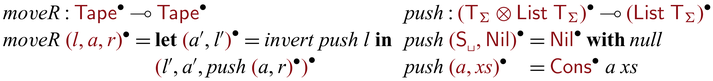
Here, ![]() is a lifted version of the tuple constructor
is a lifted version of the tuple constructor ![]() is a shorthand notation for
is a shorthand notation for ![]() , and the function
, and the function ![]()
![]() implements the inversion of a invertible function (Section 2).
implements the inversion of a invertible function (Section 2).
Then, we define the one-step transition of the given reversible Turing machine.
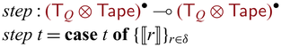
Here, the translation ![]() of each rule r is defined as below.
of each rule r is defined as below.
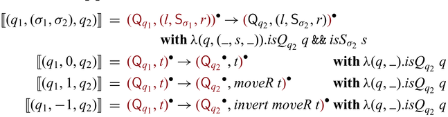
Here, ${isQ}_q : \mathsf{T}_Q \to \mathsf{Bool}$
is a function that returns
${isQ}_q : \mathsf{T}_Q \to \mathsf{Bool}$
is a function that returns $\mathsf{True}$
for
$\mathsf{True}$
for $\mathsf{Q}_q$
and
$\mathsf{Q}_q$
and $\mathsf{False}$
otherwise, and
$\mathsf{False}$
otherwise, and ${isS}_\sigma : \mathsf{T}_\Sigma \to \mathsf{Bool}$
is similar but defined for symbols. Notice that, by the reversibility of the Turing machine, patterns are nonoverlapping and at most one
${isS}_\sigma : \mathsf{T}_\Sigma \to \mathsf{Bool}$
is similar but defined for symbols. Notice that, by the reversibility of the Turing machine, patterns are nonoverlapping and at most one $\mathrel{{{{{\mathbf{with}}}}}}$
-condition becomes
$\mathrel{{{{{\mathbf{with}}}}}}$
-condition becomes $\mathsf{True}$
.
$\mathsf{True}$
.
The last step is to apply step repeatedly from the initial state to the final state, which can be performed by a reversible loop (Lutz, Reference Lutz1986). Since we do not have reversible loop as a primitive, manual reversible programming is required. In functional programming, loops are naturally encoded as tail recursions, which are known to be difficult to handle in the contexts of program inversion (Glück & Kawabe, Reference Glück and Kawabe2004; Mogensen, Reference Mogensen, Virbitskaite and Voronkov2006; Matsuda et al., Reference Matsuda, Mu, Hu and Takeichi2010; Nishida & Vidal, Reference Nishida and Vidal2011). Roughly speaking, for a tail recursion (such as $g ~ x = {{{{\mathbf{case}}}}}~x~{{{{\mathbf{of}}}}} \{ p \to g ~ e; p' \to e' \}$
),
$g ~ x = {{{{\mathbf{case}}}}}~x~{{{{\mathbf{of}}}}} \{ p \to g ~ e; p' \to e' \}$
), $\mathrel{{{{{\mathbf{with}}}}}}$
-conditions are hardly effective in choosing branches, as due to the tail call of g, the set of possible results of a branch coincides with the other’s. So we need to program such loop-like computation without tail recursions.
$\mathrel{{{{{\mathbf{with}}}}}}$
-conditions are hardly effective in choosing branches, as due to the tail call of g, the set of possible results of a branch coincides with the other’s. So we need to program such loop-like computation without tail recursions.
The higher-orderness of Sparcl (and ${{{{\lambda^{\mathrm{PI}}_{\to}}}}}$
) is useful here, as the effort can be made once for all. Specifically, we prepare the following higher-order function implementing general loops.
${{{{\lambda^{\mathrm{PI}}_{\to}}}}}$
) is useful here, as the effort can be made once for all. Specifically, we prepare the following higher-order function implementing general loops.
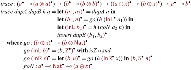
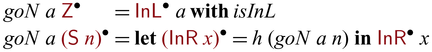
The ${trace} ~ {dupA} ~ {dupB} ~ h ~ a$
applies the forward/backward computation of h repeatedly to
${trace} ~ {dupA} ~ {dupB} ~ h ~ a$
applies the forward/backward computation of h repeatedly to $\mathsf{InL} ~ a$
; it returns b if h returns
$\mathsf{InL} ~ a$
; it returns b if h returns $\mathsf{InL} ~ b$
, and otherwise (if h returns
$\mathsf{InL} ~ b$
, and otherwise (if h returns $\mathsf{InR} ~ x$
) it applies the same computation again for
$\mathsf{InR} ~ x$
) it applies the same computation again for $h ~ (\mathsf{InR} ~ x)$
. Here, dupA and dupB are supposed to be the reversible duplication (Glück and Kawabe, Reference Glück and Kawabe2003). This implementation essentially uses Yokoyama et al. (2012)’s optimized version of Bennett (Reference Bennett1973)’s encoding. That is, if we have an injective
$h ~ (\mathsf{InR} ~ x)$
. Here, dupA and dupB are supposed to be the reversible duplication (Glück and Kawabe, Reference Glück and Kawabe2003). This implementation essentially uses Yokoyama et al. (2012)’s optimized version of Bennett (Reference Bennett1973)’s encoding. That is, if we have an injective $f : A \multimap B$
of which invertibility is made evident (i.e., locally reversible) by outputting and consuming the same trace (or, history (Bennett Reference Bennett1973)) of type H as
$f : A \multimap B$
of which invertibility is made evident (i.e., locally reversible) by outputting and consuming the same trace (or, history (Bennett Reference Bennett1973)) of type H as $f_1 : A \multimap B \otimes H$
and
$f_1 : A \multimap B \otimes H$
and $f_2 : A \otimes H \multimap B$
, respectively, then we can implement the version
$f_2 : A \otimes H \multimap B$
, respectively, then we can implement the version $f' : A \multimap B$
of which invertibility is evident by (1) copying the input a as
$f' : A \multimap B$
of which invertibility is evident by (1) copying the input a as $(a_1, a_2)$
, (2) applying
$(a_1, a_2)$
, (2) applying $f_1$
to
$f_1$
to $a_1$
to obtain
$a_1$
to obtain $(b_1, h)$
, (3) applying
$(b_1, h)$
, (3) applying $f_2$
to
$f_2$
to $a_2$
and h to obtain
$a_2$
and h to obtain $b_2$
, and (4) applying the inverse of copying (i.e., equivalence check (Glück and Kawabe, Reference Glück and Kawabe2003).) to
$b_2$
, and (4) applying the inverse of copying (i.e., equivalence check (Glück and Kawabe, Reference Glück and Kawabe2003).) to $(b_1,b_2)$
to obtain b (
$(b_1,b_2)$
to obtain b ( $= b_1 = b_2$
). Note that the roles of
$= b_1 = b_2$
). Note that the roles of $f_1$
and
$f_1$
and $f_2$
are swapped in the backward execution. Above, we use loop counts as the trace H, and go and goN correspond to
$f_2$
are swapped in the backward execution. Above, we use loop counts as the trace H, and go and goN correspond to $f_1$
and
$f_1$
and $f_2$
, respectively. The construction implies that the inverse of copying must always succeeds, and thus we can safely replace dupA by unsafe copying
$f_2$
, respectively. The construction implies that the inverse of copying must always succeeds, and thus we can safely replace dupA by unsafe copying $\lambda a.{{{{\mathbf{pin}}}}} ~ a ~ {unsafeNew}$
and dupB by
$\lambda a.{{{{\mathbf{pin}}}}} ~ a ~ {unsafeNew}$
and dupB by ${invert} ~ (\lambda b.{{{{\mathbf{pin}}}}} ~ b ~ {unsafeNew})$
. The version presented in the main body of this paper assumes this optimization.
${invert} ~ (\lambda b.{{{{\mathbf{pin}}}}} ~ b ~ {unsafeNew})$
. The version presented in the main body of this paper assumes this optimization.
By using trace, we conclude the proof by rtm below that implements the behavior of the given reversible Turing machine.
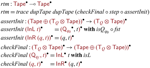
Here, ![]() is the reversible duplication of tapes. Recall that
is the reversible duplication of tapes. Recall that $q_0$
cannot be the destination of a transition and
$q_0$
cannot be the destination of a transition and $q_f$
cannot be the source. Note that, thanks to trace, the above definition of rtm is more straightforward than Yokoyama et al. (Reference Yokoyama, Axelsen and Glück2008) in which rtm is defined by forward and backward simulations of a reversible Turing machine with step counting.
$q_f$
cannot be the source. Note that, thanks to trace, the above definition of rtm is more straightforward than Yokoyama et al. (Reference Yokoyama, Axelsen and Glück2008) in which rtm is defined by forward and backward simulations of a reversible Turing machine with step counting.


 Open access
Discussions
No Discussions have been published for this article.