

1. INTRODUCTION
Ice cores are important palaeoclimate archives to reconstruct past climate changes (e.g. Petit and others, Reference Petit1999; North Greenland Ice Core Project members, 2004; Jouzel and others, Reference Jouzel2007; Jouzel, Reference Jouzel2013). Studying them improves our understanding of external forcing and feedbacks of the climate system, but for an extensive interpretation it is essential to use precise and accurate timescales. Ice cores from central Greenland are usually well dated based on annual layer counting, glaciological modelling and reference horizons as volcanic eruptions (e.g. Svensson and others, Reference Svensson2008; Sigl and others, Reference Sigl2015). However, ice from lower-altitude Arctic coring sites such as Svalbard (e.g. Isaksson and others, Reference Isaksson2005) or Severnaya Zemlya (Fritzsche and others, Reference Fritzsche2005) is subject to significant summer melt and infiltration, and requires additional climate-independent approaches to validate age models. This can be achieved by comparing decadal-scale variations of the cosmogenic radionuclide 10Be (t 1/2 = 1.387 Ma, Korschinek and others, Reference Korschinek2010), which can be considered to be globally synchronous. This approach has been successfully applied for ice cores from Greenland (e.g. Yiou and others, Reference Yiou1997; Muscheler and others, Reference Muscheler, Adolphi and Knudsen2014), Antarctica (e.g. Raisbeck and others, Reference Raisbeck1998; Muscheler and others, Reference Muscheler2007; Horiuchi and others, Reference Horiuchi2008) and, at low resolution, Franz Josef Land (Henderson, Reference Henderson2002; Kotlyakov and others, Reference Kotlyakov, Arkhipov, Henderson and Nagornov2004).
Atmospheric 10Be is produced by spallation reaction of mainly oxygen and nitrogen by high-energy particles that originate from cosmic rays (McHargue and Damon, Reference McHargue and Damon1991; Masarik, Reference Masarik and Froehlich2009). 10Be concentrations in ice cores are modulated by various processes as this cosmogenic radionuclide is transported and deposited, but solar forcing is the dominant control mechanism on the 10Be signal. Studies using principal component analysis (Steinhilber and others, Reference Steinhilber2012; Abreu and others, Reference Abreu, Beer, Steinhilber, Christl and Kubik2013) or general circulation models (Heikkilä and others, Reference Heikkilä, Beer, Abreu and Steinhilber2013) showed that the major part (>67%) of the 10Be variations can be explained by solar forcing. Another clear line of evidence for the solar influence is the presence of the prominent 11-year Schwabe solar cycle and the grand solar minima that resulted in an increase of mean 10Be concentrations by 30–50% (Bard and others, Reference Bard, Raisbeck, Yiou and Jouzel2000). In particular, these non-periodic fluctuations with a length of approximately 60–100 years are helpful when synchronizing 10Be records from different archives. Therefore, an appropriate temporal resolution has to be chosen that allows the identification of these prominent features but attenuates shorter, locally specific fluctuations. Steinhilber and others (Reference Steinhilber2012) and Muscheler and others (Reference Muscheler, Adolphi and Knudsen2014) found that local fluctuations are reduced to 20–30% of the total signal when averaging over 20–25 years. However, spikes in 10Be concentrations that are related to single solar/cosmic events such as CE (Common Era) 774/75 (Mekhaldi and others, Reference Mekhaldi2015; Miyake and others, Reference Miyake2015; Sigl and others, Reference Sigl2015) are only of short duration. In order to distinguish such outstanding events from short, local fluctuations, it is necessary to consider that deviations from the solar signal might arise in production, transportation and deposition of 10Be. Variations of the geomagnetic field influence the production on a millennial timescale, but are generally low in Polar Regions (Beer and others, Reference Beer2002). In contrast to stratospheric 10Be production (~2/3 of total production), the 10Be produced in the troposphere (1/3) introduces a more local to regional signal, because the shorter residence time of some weeks precludes global mixing. A rapid change in the deposition mechanism that can be either via precipitation (wet deposition) or settling out directly from the air (dry deposition) might also be misleading. However, modelling the concentration of 10Be using atmospheric circulation models showed that the production signal is preserved despite striking climate changes (Alley and others, Reference Alley1995; Heikkilä and others, Reference Heikkilä, Beer and Feichter2008). Finally, local, post-depositional alteration of 10Be concentration in the snow cover may occur due to summer melting followed by percolation. The effects of melting and infiltration on 10Be are yet not well-investigated but assumed to be small after averaging over a few years (Pohjola and others, Reference Pohjola2002).
The Akademii Nauk (AN) ice core is the most easterly of those from the Eurasian Arctic, an area generally lacking high-resolution palaeoclimate records from the Late Holocene. The existing age model of this ice core is based on annual-layer counting and reference horizons (Opel and others, Reference Opel, Fritzsche and Meyer2013). Here, we present an independent 10Be-based approach to validate and extend the age model and show a new mid-resolution 10Be record for the period CE 1590–1950. Furthermore, we developed an adjusted core-sampling strategy for the remaining ice core sections.
2. STUDY SITE AND AN ICE CORE
The Severnaya Zemlya Archipelago in central Russian Arctic represents the most easterly location suitable for ice core drilling in the Eastern Arctic (Fig. 1). Soviet scientists have drilled ice cores since the 1970s at Vavilov and AN ice caps (Kotlyakov and others, Reference Kotlyakov, Arkhipov, Henderson and Nagornov2004). Although their chronologies covered Late Pleistocene ages for the deepest ice core sections close to bedrock, the results were questioned by Koerner and Fisher (Reference Koerner and Fisher2002), who suggested a Late Holocene age after a near complete melting of the ice caps during the Early Holocene thermal optimum. To resolve the maximum age and to retrieve new high-resolution palaeoclimate records using modern ice core analytical methods, a new 724 m long ice core was drilled in 1999–2001, close to summit of the dome-shaped AN ice cap at Komsomolets Island (80.52°N, 94.82°E), ~750 m a.s.l. (Fritzsche and others, Reference Fritzsche2002).
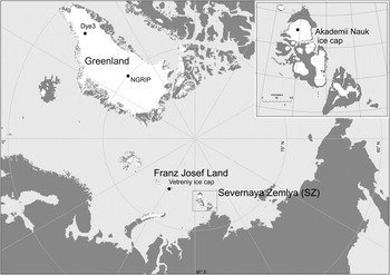
Fig. 1. Map of the Arctic with locations of the discussed 10Be records from Akademii Nauk, Dye3, NGRIP and Franz Josef Land ice cores.
Due to the low altitude of the drilling site, temperatures in summer may exceed 0°C and cause melting of the surface snow and subsequent infiltration of the meltwater into deeper layers (Opel and others, Reference Opel2009). Hence, the AN ice core consists of alternating sections of firn, partly infiltrated firn and pure melt layers (Fritzsche and others, Reference Fritzsche2005). Melting and infiltration redistribute major ions and other species as trace elements and disturb the original signal of seasonal deposition (Weiler and others, Reference Weiler2005). However, as stable-isotope ratios still show seasonal variations, even though muted in most cases, the impact of melting, infiltration and refreezing is considered to be minor. On annual to multi-annual timescales, the AN ice core is suitable for high-resolution studies of palaeoclimate and atmospheric aerosol loading (Opel and others, Reference Opel, Fritzsche and Meyer2013; Spolaor and others, Reference Spolaor2016).
The chronology of the upper section (0–411 m) of the AN ice core (Opel and others, Reference Opel, Fritzsche and Meyer2013) is based on reference horizons and annual-layer counting (seasonal variations of stable isotopes). As reference horizons we used the 1963 137Cs peak caused by fallout from nuclear bomb tests (Fritzsche and others, Reference Fritzsche2002; Pinglot and others, Reference Pinglot2003; Arienzo and others, Reference Arienzo2016) as well as volcanic signals. As the assignment of SO4 2− peaks to distinct volcanic eruptions might be ambiguous in some cases, an independent method is required to validate and extend the age-depth model of AN ice core.
The mean modern accumulation rate was 0.46 m w.e. a−1 over the period 1956–1999. A basal ice layer ~30 m thick has physical and chemical properties that differ from the upper parts of the ice core, and is likely a relict of a former stage of the ice cap. Using a common 1-D flow model after Nye (Reference Nye1963) with a constant accumulation rate of 0.46 m w.e. a−1 and a glacier thickness of 660 m w.e., we assumed that the undisturbed ice core above the basal ice covers ~4600 years, given that the glacier has been in steady state. This maximum age will decrease if a non-steady state with an increasing altitude of the ice cap surface is assumed. Kotlyakov and others (Reference Kotlyakov, Arkhipov, Henderson and Nagornov2004) published ages between 10 and 40 ka for near-bottom ice layers of AN and Vavilov ice caps, but δ18O and δ2H values from AN ice core clearly point to a warm, interglacial climate and therefore a Holocene age (Opel and others, Reference Opel, Fritzsche and Meyer2013).
3. METHODS
3.1. Sample preparation
The ice core processing and sampling scheme is described in Fritzsche and others (Reference Fritzsche2005). After measuring density and electrical conductivity by dielectric profiling, we took one sample for stable isotope analysis and a second sample for line-scanning and glaciochemistry. From the remaining ice of the second sample we selected 77 discontinuous samples from the upper part of the ice core (core depth 29.43–183.00 m, corresponding to CE 1590–1950 using our age model presented in Opel and others, Reference Opel, Fritzsche and Meyer2013). Individual sample lengths varied between 0.21 and 1.22 m (mean 0.70 m), corresponding to 0.32 and 3.05 years (mean 1.65 years), respectively.
To isolate beryllium, the 77 ice core samples (216–569 g) were chemically treated at the DREAMS (DREsden Accelerator Mass Spectrometry) facility of the Helmholtz-Zentrum Dresden-Rossendorf. Samples were prepared in batches of up to nine, accompanied by a processing blank, which was treated identically as the corresponding ice samples but based on deionized H2O (18 MΩ) and ~0.3 ml 9Be-carrier (Scharlau, Batch 11863301; 2% HCl, 9Be concentration of (980.4 ± 4.9) μg g−1). The method was developed from original work at the University of Heidelberg (Stanzick, Reference Stanzick1996; personal communication from D. Wagenbach, 2009). The main steps were: (a) melting ice in a polypropylene beaker containing ~300 µg of a 9Be-carrier and ~1 ml of hydrochloric acid (10.2 M) (at room temperature); (b) adjustment of pH to 4 by ammonia solution (25%); (c) binding of Be2+ onto a cation ion exchange column (Bio-Rad; DOWEX 50Wx8; 100–200 mesh; 8 mm diameter; 40 mm long); (d) release of Be2+ by 25 ml HCl (1 M); (e) precipitation of Be as hydroxide by ammonia solution (25%); (f) repeated rinsing (3 times) with very dilute ammonia solution (pH 8–9); (g) drying and ignition to BeO at 900°C and (h) addition of and mixing with Nb-powder (1:4 to 1:6 (BeO:Nb) by weight) and pressing into copper target holders.
3.2. AMS measurements of 10Be
The DREAMS-facility (Akhmadaliev and others, Reference Akhmadaliev, Heller, Hanf, Rugel and Merchel2013; Rugel and others, Reference Rugel2016) was used between 2011 and 2016 to determine the 10Be/9Be ratios in each sample. Measurements were performed in the same batches as the chemical treatment. They included the corresponding processing blanks to take into account the amount of 10Be resulting intrinsically from the 9Be-carrier and cross contamination while chemical processing and within the AMS ion source. Results were quantified versus the in-house-standard SMD-Be-12 with a nominal 10Be/9Be of (1.704 ± 0.030) × 10−12.
3.3. Processing of data
Each 10Be concentration data point was assigned to an age span according to its sample depth. To reduce the influence of short-term fluctuations and aliasing of the 11-year cycle from non-continuous measurements, the data were averaged over 22 years, weighted by their respective age-span (cf. McCracken and others, Reference McCracken, McDonald, Beer, Raisbeck and Yiou2004; Berggren and others, Reference Berggren2009; Steinhilber and others, Reference Steinhilber2012). The 22 year averaged AN 10Be record was then correlated to 22 year averages of the Dye3 (Beer and others, Reference Beer1990) and NGRIP (Berggren and others, Reference Berggren2009) records using the Pearson correlation coefficient. We further analysed the correlation in a sliding 50-year window to investigate temporal changes in the relationship.
For significance testing we resampled the original 10Be data 1000 times using block bootstrap resampling (Sherman and others, Reference Sherman, Speed and Speed1998), creating independent time series with the same distribution and autocorrelation structure as the original dataset. This surrogate data were handled as the original dataset by taking 22 year means and calculating (running) correlations. We then used the 5 and 95% quantiles of the correlation distribution to provide the thresholds for local significance. For the running correlation, the difference in the resulting thresholds for AN versus Dye3 and AN versus NGRIP, as well as their time dependency are very small (<0.05) and we therefore show one single significance threshold in Figure 4. It is known that running correlations tend to show strong correlation changes over time, even if the underlying relationship is stationary (Gershunov and others, Reference Gershunov, Schneider and Barnett2001; van Oldenborgh and Burgers, Reference van Oldenborgh and Burgers2005).
Thus we further tested whether the changes in correlation over time are statistically significant using the approach of van Oldenburg and Burgers (Reference van Oldenborgh and Burgers2005). For this test, the maximum change in the running correlation over time was compared with the maximum change obtained in a pair of time series that have by construction a time-invariant correlation. Therefore, the Dye3 or NGRIP data were replaced by synthetic observations having the same mean correlation to the 22 year AN series as our sample estimate and which further preserve the autocorrelated residuals that are caused by the 22 year running mean filter.
3.4. Numerical model for core-sampling strategy
We aimed to develop a core-sampling strategy that minimizes artefacts in the resulting 10Be series. For example, aliasing can occur when a sampling frequency is too low to reconstruct all variations. To identify the optimal strategy, we analysed the impact of different core-sampling strategies on the record by means of a numerical simulation. We resampled an existing record at different spacing and coverage, reconstructed a new time series and compared it with the original (Fig. 2). For the simulations, we used 10Be records from Dye3, NGRIP and Dome Fuji (Beer and others, Reference Beer1990; Horiuchi and others, Reference Horiuchi2007, Reference Horiuchi2008; Berggren and others, Reference Berggren2009) but only show the Dye3 results as the results of all the three datasets are very similar. Details of the theoretical considerations and the numerical model are presented in the Supplementary Material 1.

Fig. 2. Modelling procedure (a–c) and results (d–e): (a) Dye3 original data with two example sampling strategies: continuous samples of 8-years length (green) and samples of 0.1-years length taken every 3 years (red). For the samples consisting of more than one data point the average of all points within the sample interval is taken. (b and c) 22-years running mean from the original dataset (black line) compared with samples following the abovementioned sampling strategies and the corresponding 22-years running means, continuous samples of 8-years length (b), samples of 0.1-years length taken every 3 years (c). (d and e) Correlation coefficients (black dots) for multi-year sampling (d) and single-point sampling (e).
First, two different modes of sampling were distinguished: point sampling, representing a single moment in time (e.g. samples a few centimetres long corresponding to a few months); and multi-year sampling, representing information spanning a few years (samples up to a few metres long). In both modes, different sample periods between 1 and 22 years were tested. For single-point sampling a single value was taken, but the longer samples were averaged over more data points. To simulate age-model uncertainties caused by fluctuations in the accumulation rate, each sampling step was biased by adding a uniformly distributed random number on the interval −10 to 10 representing a change of ±1 year to the original time span. Furthermore, a modification of the multi-year sampling process has been developed to simulate missing parts in the ice core. Here in 50% of the cases, the end point of the interval is shifted by a random amount of 0–2 years (uniform distribution). Then a 22-year running mean was applied to the points of each sample run.
The degree of consistency of the sample records was evaluated with the Pearson correlation coefficient for the 22-year running mean of the original dataset and the one of the reconstructed curve. Finally, procedure was performed repeatedly (50 runs) and the mean of the correlation is reported. The outcome of the model was used to develop a sampling strategy that generates a suitable AN 10Be average concentration record for matching with well-dated 10Be records from Greenland ice cores.
4. RESULTS AND DISCUSSION
4.1. 10Be concentrations in the AN ice core
Beryllium-10 data are presented in Table S1 (Supplementary Material 2) and Figure 3. Total uncertainties from the AMS measurements are based on counting statistics and the uncertainty of the standard, summing up to 2.3–14.2% (average 3%). The total uncertainty budget also includes a blank-correction of 0.3–14.1% (average 1.4%) and an uncertainty of 0.5% from the 9Be concentration of the carrier. Beryllium-10 results in units of atoms g−1 are calculated from the amount of 9Be (~2 × 10¹⁹ atoms) from the carrier addition and the weight of the ice sample. Standard uncertainties (1-sigma) are given for 10Be results.
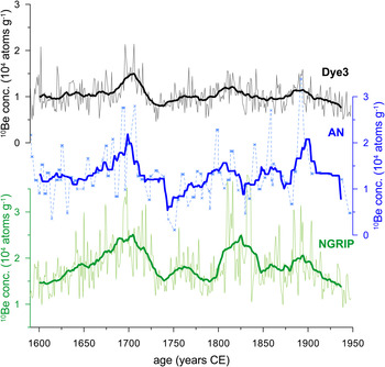
Fig. 3. 10Be records of Dye3, AN and NGRIP. The original datasets of Dye3, NGRIP (Beer and others, Reference Beer1990; Berggren and others, Reference Berggren2009) and AN (individual samples, this work) are displayed as thin lines together with the corresponding 22-years running means (bold lines) for the time span CE 1590–1950.
The 10Be concentration of the AN ice core samples ranges between 1.12 × 10³ and 3.38 × 10⁴ atoms g−1, with an average of 1.31 × 10⁴ atoms g−1 and a coefficient of variation of 0.38 (Fig. 3). Some of these variations can be attributed to the grand solar minima. For example, the maximum at ~CE 1700 corresponds with the Maunder Minimum. The maximum at CE 1820 could be attributed to the Dalton minimum followed by another peak at ~CE 1850 that could not be assigned to a grand solar minimum. Another, very distinct maximum occurs at ~CE 1910 followed by a decline in concentration.
4.2. AN 10Be record compared with Dye3 and NGRIP
The overall agreement of the AN, Dye3 and NGRIP 10Be records, in terms of concentration and temporal pattern of variations confirms the reliability of the 10Be concentrations of the AN ice core (Fig. 3). The AN and Dye3 records show general accordance, confirmed by a correlation coefficient of r = 0.59, p = 0.003 (Pearson correlation coefficient for running means over 22 years, p-value accounting for autocorrelation in 10Be as well as the running mean, see Section 3.3). The running means over 22 years of the AN and NGRIP records correlate with r = 0.45, p = 0.01. Interestingly, shifting the chronology of AN in either direction by any value only decreases the correlation of 10Be to both Greenlandic ice cores thus providing a validation of the current chronology.
The stronger relationship between AN and Dye3 might imply that both cores share more common influences on their 10Be than AN with NGRIP. Since snow accumulation at AN is high and similar to Dye3 (~0.5 m w.e. a−1; Sturevik-Storm and others, Reference Sturevik-Storm2014), 10Be deposition mainly takes place via wet deposition while for the NGRIP record (accumulation rate of ~0.19 m w.e. a−1; Sturevik-Storm and others, Reference Sturevik-Storm2014) dry deposition might play a larger role. In addition to deposition mechanisms, the altitude, latitude and also the distance from the coast may further introduce local fluctuations (Heikkilä and others, Reference Heikkilä, Beer and Feichter2008; Berggren and others, Reference Berggren2009) and NGRIP is at higher altitude and more distant from the coast than AN and Dye3.
Using running correlations with a window of 50 years we could identify three intervals of high correlation between AN and Dye3 10Be records that are interrupted by two, shorter deviations at ~CE 1750 and ~CE 1850 (see Fig. 4). In the oldest part of the core (~CE 1650) the correlation is also weaker. A similar pattern was found for AN-NGRIP but with larger and longer deviations. While parts of these changes in the correlation over time are expected from statistical reasons (Gershunov and others, Reference Gershunov, Schneider and Barnett2001), a significance test (Section 3.3) shows that the changes we observe for AN versus Dye3 are unlikely to only have occurred by chance (p = 0.06 for AN-Dye3 and p = 0.14 for AN-NGRIP). Thus, the deviations that cause lower or even negative correlations require further interpretations.

Fig. 4. 50-years running correlation of the 10Be records of AN versus Dye3 and AN versus NGRIP. The running correlations are shown in black (AN-Dye3) and blue (AN-NGRIP). The sample density (percentage of the 50-year window that was sampled) is shown in green. Local significance levels (p = 0.05) are shown as horizontal dashed line.
Possible reasons for the reduced correlations are (1) single, short events leading to outliers, (2) local fluctuations, (3) uncertainties due to sampling that we now discuss in detail.
-
(1) Outliers from short-term variations in transport, deposition or post-depositional change of the 10Be concentration could affect the inter-site correlation. To test this hypothesis, we identified extreme values with a normal probability plot and removed them stepwise. However, the removal of outliers only lowered the correlation. Therefore, we deduced that these samples represent a depositional signal (e.g. extremes of the 11-year solar cycle) rather than local fluctuations, and they are important for reconstructing the production signal.
-
(2) Local fluctuations in 10Be might reduce the correlation between AN and the Greenlandic sites. Indeed, we observed that the periods with lower correlation coefficients coincide with periods when the Dye3 and NGRIP 10Be time series are less variable. Such intervals might be more sensitive to local effects on 10Be such as changes in the percolation of the AN ice core record or changes in air transport patterns (Muscheler and others, Reference Muscheler, Adolphi and Knudsen2014). According to Steinhilber and others (Reference Steinhilber2012), the local variations, which make up to 30% of the signal, are probably the main reason for differences between different records of radionuclides. A similar temporal pattern of the correlation was detected in the AN-Dye3 as well as in the AN-NGRIP relationship, supporting that a local- to regional-scale event like strong summer melt and infiltration on the AN ice cap may explain this deviation.
-
(3) Uncertainties can also be introduced due to the sampling scheme and reconstruction procedures (Berggren and others, Reference Berggren2009; Beer and others, Reference Beer, McCracken and von Steiger2012; Muscheler and others, Reference Muscheler, Adolphi and Knudsen2014). For example, McCracken (Reference McCracken, Kajita, Asaoka, Kawachi, Matsubara and Sasaki2003, Reference McCracken2004) showed that aliasing effects due to an unresolved 11-year cycle could be the largest source of noise in a 10Be record (up to 35%). To better understand the impact of sampling-related uncertainties on the AN record, we analysed the sample distribution of the AN core. On an average, 37% of the core was sampled. The sample density increases continuously from 20% ~1930 up to 59% in the earliest part of the core (Fig. 4). On average, samples cover a time of 1.65 years and there are ~25 samples per 100 years.
To investigate the effect of sampling, we used numerical simulations (described in Section 3.3), as the number of actual samples of the AN ice core is insufficient to allow a direct test on the dataset. The results (Fig. 2d, e) show that continuous sampling using multi-year samples leads to a better reconstruction of the 10Be long-term variations than using point samples at high resolution. This suggests that at least when aiming to maximize the correlation between 10Be records it is more important that no information is lost (continuous sampling), than having a high temporal resolution. Interestingly, also the model run including simulated gaps has a high agreement when sampled continuously (not shown). Therefore, we concluded that continuous sampling is the most powerful sampling method and can be applied successfully even on ice cores that are incomplete.
The actual mean sample density of 37% and mean time span of 1.65 years in our core are somewhere between the two extreme cases of continuous (multi-year) and single-point sampling. This result supports those of other authors (Yiou and others, Reference Yiou1997; Henderson, Reference Henderson2002) that dating with 10Be can be achieved despite gaps in the record. However, the mean time span of 1.65 years in our dataset appears to be quite short compared with other, non-continuously sampled ice cores. For example, Henderson (Reference Henderson2002) used individual samples covering a time span of 7–8 years from Franz Josef Land ice core. Our simulations indicate higher variability in the reconstruction quality when using shorter samples. Thus the sampling procedure might have contributed to lowering the correlation between AN and Greenland ice cores.
4.3. Strategy for future ice core sampling
10Be concentrations, mainly analysed for solar or geomagnetic studies, have been used to synchronize ice cores from different hemispheres or different archives as tree rings and sediments. However, sampling strategies for studies focusing on the validation of age models are largely missing. The initial sampling scheme resulted in a 10Be record with a correlation of 0.59 to the Dye3 record but might not have been optimal. This might also be responsible for missing correlations (see Section 4.2). Therefore, a future sampling strategy for extending the 10Be record, i.e. for deeper parts of the AN ice core is developed based on the results of the numerical model (see Section 3.4). Robust reconstruction results are achieved for continuous sample lengths covering a time span of 4–8 years and 22 years (Fig. 2d). The latter can be explained by the fact that aliasing is completely suppressed. The intermediate sample length seems to be an optimum between two competing processes. On the one hand, shorter samples allow a finer reconstruction, whereas on the other, taking longer samples attenuates outliers, but also aliasing effects due to melting and percolation lead to a ‘pre-averaging’ (Wunsch, Reference Wunsch2000). This competition, combined with the irregular period of the 11-year solar cycle might also explain why the optimum is not 11 years, but shifted towards shorter samples, yielding a maximum at ~8 years. These intermediate sample lengths lead to the highest correlation and the smallest standard deviation, and so they provide a reliable and reproducible approach for reconstruction. Using uneven sample intervals could further reduce the magnitude of aliased peaks, as shown in a numerical simulation by Pisias and Mix (Reference Pisias and Mix1988). This is common practice for ice cores sampled in constant depth intervals, leading to varying time intervals, for example GRIP (Yiou and others, Reference Yiou1997), Vostok (Raisbeck and others, Reference Raisbeck1998) and Dome Fuji (Horiuchi and others, Reference Horiuchi2008). Sampling at constant depth intervals corresponding to ~4 years in the younger parts of the ice core, but to up to 8 years in the lower part might be a good way to combine uneven sample intervals with the optimal sample lengths found by the model, especially as variations in the accumulation rate will naturally lead to variations in the effective time period covered by the samples.
Nonetheless, the procedure outlined above might not be feasible for all 10Be ice core studies. There are practical issues favouring fewer and shorter samples. Continuous sampling is time consuming. Also, in the case of AN, the compatibility of new samples with former samples might be worse when changing from shorter to longer samples. That is why one has to consider carefully the extent to which the existing strategy should be adopted.
We propose adjusting the sampling strategy as follows. First, one should identify parts of the record known to be difficult to reconstruct (e.g. where there is little variation) or that require absolute reliability (e.g. cosmic events). Second, one should use longer, continuous samples (corresponding to at least 4 years) in these parts.
5. CONCLUSIONS AND OUTLOOK
-
(1) The existing age model of the AN ice core was validated by a climate-independent approach using the concentration of the cosmogenic radionuclide 10Be. The 77 individual 10Be data points have been averaged over 22 years to reduce aliasing influences and local, climate induced differences in the 10Be dataset before comparing them to the Dye3 and NGRIP 10Be records.
-
(2) An overall high correlation coefficient of r = 0.59 (p = 0.003) between AN and Dye3 suggest that the AN 10Be concentrations reflect the production signal and are, therefore, suitable for dating. Furthermore, it validates the existing ice core chronology of AN. This is supported by a decrease in correlation for any shifts applied to the AN age model.
-
(3) At ~CE 1650, 1750 and 1850 there are short periods of weak or even negative correlations. These deviations seem to coincide with time-periods of reduced variability in 10Be and are likely caused by local fluctuations of 10Be transport, deposition and preservation. Numerical simulations of the sampling strategy suggest that the current sampling procedure might also have caused a reduction in the reconstruction quality. Further sampling will be performed based on a new sampling strategy using longer samples to exclude sampling itself as an error source.
-
(4) Sampling of the remaining 75% of the core will be continued to constrain a core chronology for the deeper ice core part to fully explore the potential of the AN ice core for reconstruction of climate and environmental changes in the Eastern Arctic over the Late Holocene.
SUPPLEMENTARY MATERIAL
To view supplementary material for this article, please visit https://doi.org/10.1017/jog.2017.19
ACKNOWLEDGEMENTS
Parts of this research were carried out at the Ion Beam Centre (IBC) at the Helmholtz-Zentrum Dresden-Rossendorf e. V., a member of the Helmholtz Association. Insightful discussions with D. Wagenbach (Heidelberg University, deceased) and his generous support are highly appreciated and valued. We thank Andreas Scharf, Shavkat Akhmadaliev and Santiago M. Enamorado Baez for their support to AMS measurements. The chemical sample preparation has been supported by Vicki Kühn, Malin Lüdicke, Stephanie Uhlig, Hannes Wenzel and René Ziegenrücker. We thank Jürg Beer for providing the Dye3 data. We are grateful to Julian Murton and two anonymous reviewers for valuable comments, hints and language correction that helped to improve the quality of the manuscript. This study contributes to the Eurasian Arctic Ice 4k project (grant OP 217/2–1 by the Deutsche Forschungsgemeinschaft awarded to Thomas Opel) and the ECUS project (Initiative and Networking Fund of the Helmholtz Association, grant VH-NG-900).
AUTHOR CONTRIBUTIONS
L.v.A., T.O. and D.F. designed the study. L.v.A., T.O. and D.F. performed ice core sampling. L.v.A., S.M. and G.R. prepared and analysed the 10Be samples. L.v.A. performed model calculations, T.L. performed the running correlation and significance estimates. All authors contributed to the final discussion of the obtained results and interpretations and the preparation of the manuscript.10Be data are available at https://doi.org/10.1594/PANGAEA.869948


 Open access