

1. INTRODUCTION
Glaciers in high altitude, mountainous regions are a highly important source of fresh water for major river systems (Li and Williams, Reference Li and Williams2008; Immerzeel and others, Reference Immerzeel, Petersen, Ragettli and Pellicciotti2014); however, modelling the future availability of such resources is often hampered by insufficient data or poor understanding of localised meteorological conditions. Near-surface air temperature (T a), typically measured at a height of 2 m, is considered the most important control on energy exchange over a snow or ice surface (Petersen and others, Reference Petersen, Pellicciotti, Juszak, Carenzo and Brock2013) due to its controls on many components of the energy balance. However, the spatial distribution of this variable over glaciers is unknown and thus often estimated from a single off-glacier location using simple, uniform lapse rates.
Lapse rates (referred to here as temperature gradients (TGs)), which define a variable dependency on elevation, are the most common method of distributing T a in model studies (Marshall and others, Reference Marshall, Sharp, Burgess and Anslow2007; Petersen and Pellicciotti, Reference Petersen and Pellicciotti2011; Wheler and others, Reference Wheler, Macdougall, Petersen and Kohfeld2014). An environmental ‘lapse rate’ (ELR = −0.0065°C m−1) is often applied in the absence of measured values to extrapolate T a across a glacier (Arnold and others, Reference Arnold, Rees, Hodson and Kohler2006; Machguth and others, Reference Machguth, Paul, Hoelzle and Haeberli2006; Nolin and others, Reference Nolin, Phillippe, Jefferson and Lewis2010). The application of a temporally constant and spatially homogenous free-air TG has, however, been questioned for glacierised basins, particularly at high altitude where the effect of terrain cannot be neglected (Marshall and others, Reference Marshall, Sharp, Burgess and Anslow2007; Gardner and others, Reference Gardner2009; Minder and others, Reference Minder, Mote and Lundquist2010; Petersen and others, Reference Petersen, Pellicciotti, Juszak, Carenzo and Brock2013).
Marshall and others (Reference Marshall, Sharp, Burgess and Anslow2007) identify that both surface and atmospheric conditions affect the spatio-temporal patterns of T a and a constant single station TG may not account for these changes. Above a melting debris-free ice surface, the variations in TGs have been documented to become less negative (i.e. reflect smaller changes of T a with elevation) as a result of katabatic development in the boundary layer (Greuell and Böhm, Reference Greuell and Böhm1998; Shea and Moore, Reference Shea and Moore2010; Petersen and Pellicciotti, Reference Petersen and Pellicciotti2011; Ayala and others, Reference Ayala, Pellicciotti and Shea2015). As many studies force models from off-glacier locations, the T a variability within the katabatic boundary layer is often unaccounted for, lending to overestimation of temperatures when extrapolated on glacier (Shea and Moore, Reference Shea and Moore2010). While little is known about the development of meteorological conditions over debris-covered glaciers, katabatic winds are generally absent due to the lack of a 0°C surface and the movement of air being dominated by surface convection from debris cover heating under fine conditions (Brock and others, Reference Brock2010). A number of factors are considered to affect T a over debris cover such as debris thickness (Foster and others, Reference Foster, Brock, Cutler and Diotri2012), wind speed and topographic exposure (Fujita and Sakai, Reference Fujita and Sakai2000; Brock and others, Reference Brock2010) though data have typically been limited to a few automatic weather station (AWS) sites.
The vertical TG averaged between two AWS on Miage Glacier was found to be −0.0080 for the 2006 ablation season though with considerable temporal variations attributable to differential debris heating resulting from topographical shading and time of day (Brock and others, Reference Brock2010). Similar average TGs (−0.0075°C m−1) were found by Mihalcea and others (Reference Mihalcea2006) on Baltoro Glacier, Karakoram. The authors found that TGs over Baltoro Glacier were more negative during the evening and at night and became less negative during the day, partially connected to the variability in wind speed.
Thicker supraglacial debris has been found to lead to higher T a over debris-covered glaciers (Brock and others, Reference Brock2010; Foster and others, Reference Foster, Brock, Cutler and Diotri2012). Brock and others (Reference Brock2010) conclude that T a variations on Miage Glacier are dominated by convective heating from the debris surface, though they only assess T a from two AWS locations. Fujita and Sakai (Reference Fujita and Sakai2000) found more negative TGs over debris-covered compared with debris-free areas of Lirung Glacier, Nepal Himalaya. TGs were more negative over debris during the day as a result of the storage and release of heat from the debris layer. This is in contrast to the findings of Mihalcea and others (Reference Mihalcea2006). However, this difference is also controlled by variations in meteorological and surface conditions, whereby cloudy and wet conditions and areas of thinner debris reduce the convective influences. Difficulty in parameterising T a TGs over debris is therefore exacerbated by the formation of cloud in high altitude mountain environments as well as the variations in debris thickness and surface features such as crevasses and ice cliffs (Han and others, Reference Han, Wng, Wei and Liu2010; Reid and Brock, Reference Reid and Brock2014).
While some studies have increased the understanding of T a distribution across debris-free glaciers by using more observations (i.e. Petersen and Pellicciotti, Reference Petersen and Pellicciotti2011; Ayala and others, Reference Ayala, Pellicciotti and Shea2015), to our knowledge, only one study has provided such a quantity of data for debris-covered glaciers (Ragettli and others, Reference Ragettli2015) and none have investigated the importance of debris cover to an energy-balance model. This work therefore aims to address these issues by employing a dense network of stations over an Alpine debris-covered glacier to understand the spatio-temporal variability of T a, identify its main controls and physical drivers and evaluate its impact on modelled melt totals.
2. STUDY SITE
Miage Glacier is a large (~9.5 km2) valley glacier in the Western Italian Alps, located at the southwest flank of the Mont Blanc Massif (45°47′N, 06°52′E). Miage Glacier has steep tributaries feeding its main body; Dome Glacier, Bionnassay Glacier and Tête Carrée Glacier. It has an elevation range of ~2900 m with its lowest elevation at 1736 m. The glacier follows a northwest to southeast direction confined by the valley walls until it enters Val Veny, whereby it bends towards the northeast and splits into three lobes. The lower tongue (comprising a northern, southern and smaller central lobe) is flanked by lateral moraines up to 200 m high (Deline, Reference Deline2005). Of the 9.5 km2 area of the glacier, ~4.5 km2 is covered by continuous debris cover, with 4.6 km2 classified as ‘clean’ ice or snow and the remaining transitional area (0.3 km2) referred to as dirty ice (Fyffe and others, Reference Fyffe2014). The continuous debris mantle comprises a mix of lithology, mainly dominated by gneiss, schist and granite.
3. DATA
3.1. Meteorological data
Near-surface T a were measured across the glacier at 18 locations with Gemini Tinytag (TT) dataloggers (Fig. 1, Table 1) with standard PB-5001 thermistor probes or temperature relative humidity (T-RH) probes (accuracy ±0.20 and ±0.35°C, respectively). Each probe was housed in naturally ventilated Campbell Scientific MET20/21 radiation shields and mounted on a 2 m Onset tripod (Fig. 2). All stations including an off-glacier (OG) site covered an elevation range of ~750 m (Fig. 3).

Fig. 1. Map of the Miage Glacier with the positions of TT(n) stations, INT3 setup and surface classification. Inset shows position within Western Europe. Contours are shown in 300 m intervals.

Fig. 2. (a) TT13 as an example of the temperature station in the field (image taken 14:20, 30th June, 2014) and (b) OG station and ground conditions.

Fig. 3. Longitudinal profile of the Miage Glacier given as the distance from the north lobe terminus (m) and the relative locations of AWS and TT stations. The peak at ~1400 m is the result of large debris deposits on the glacier bend. Elevation data are derived from a 2010 Lidar survey. Note: vertical scale is exaggerated.
Table 1. Miage Glacier TT/AWS station setup and descriptive statistics

Elevation recorded by Trimble Juno handheld GPS. T–RH, air temperature and RH sensor; Dual, air and surface temperature sensors. UWS T–RH is provided by a Vaisala HMP-45A sensor.
Distributed T a data were supported by two full energy-balance AWS on the upper (UWS) and lower (LWS) glacier with similar instruments to those used by Brock and others (Reference Brock2010) and Fyffe and others (Reference Fyffe2014). The common observation period of this investigation was 1 July until 27 September 2014 (89 days). Hardware failure resulted in the absence of LWS data throughout July (excluding T a measured by a TT logger) and as such, LWS data were only provided from 1 August onwards. UWS data were available for the full observation period. TT data were sampled every 5 s and recorded in 10 min intervals. AWS data were sampled every 1 s and logged in 30 min intervals. All data were averaged into hourly values for analysis. Precipitation data were provided by the Regione Autonoma Valle d'Aosta AWS proximal to the Lex Blanche (LB) Glacier (2162 m, ~4 km west of LWS).
3.2. Air temperature inter-comparison
In order to ensure accurate quantification of differences in T a measured between sites on the glacier, TT loggers were tested under near-identical conditions for 3 different inter-comparison tests. The first 2 tests (INT1 and INT2) were able to assess the differences in T a recorded under receipt of high shortwave radiation (clear skies) and absence of wind which generally promotes the highest errors associated with the radiation shield type (±0.50 and ±0.75°C for MET21 and MET20, respectively). Multiple TT thermistors were housed in single radiation shields and mounted to the same tripod, recording 10 min values for a 24 h period. These tests revealed maximum T a differences to be ~0.14°C, within the manufacturer error range for the loggers (±0.20°C). INT3 was conducted prior to on-glacier setup, in the pro-glacial area at La Visaille from 7–9 April 2014 (Fig. 1), logging at 10 minute intervals. This test was conducted for a 40 h period during mixed weather conditions and overlying continuous snow cover in a forest clearing. The results of INT3 revealed larger variations in T a between loggers, likely the result of difficulty in gaining near-identical testing conditions for all sensors and the role of localised shading from trees. Differences were largest for a rapid transition from cloudy to clear sky conditions, which demonstrated the differences >1°C for the less accurate T-RH loggers, though were considerably less when averaged into hourly values consistent with the on-glacier measurements in this study (maximum differences ~0.40°C). However, excluding this short period of time, differences remained close to the manufacturer error, and thus the values given by these loggers can be considered reflective of the T a variations across Miage Glacier. The logger type and radiation shield for each station is provided in Table 1.
3.3. Ablation data
At each temperature station a low conductivity 2 m PVC stake was used as a measure of ablation for the common observation period. The stakes were typically located within ~10 m of the temperature station in an area that was relatively flat but also as representative as possible of the debris surface characteristics beneath the station. The debris was removed to allow holes to be drilled into the ice using a strengthened Kovacs ice drill, the initial depth of the stake was measured from the top to the surface of the ice and the debris was replaced as naturally as possible. Water equivalent ablation for the 14 stakes was calculated assuming an ice density of 890 kg m−3 (Brock and others, Reference Brock2010; Fyffe and others, Reference Fyffe2014). For TT14, initial stake drilling was into thick snow cover. Snow ablation was converted to water equivalent using the snow density gained from measurements at TT2 in April 2014, averaging 510 kg m−3 from a 60-cm deep snow pit. Dates of ablation measurements are shown in Table 2.
Table 2. Ablation stake measurement periods given for each stake at the corresponding TT station in dd.mm

Missing values indicate where full melt out of the stakes had occurred.
4. METHODS
4.1. TG analyses
To establish the effect of differing meteorological conditions on near-surface T a gradients, the data were stratified according to temperature, cloud conditions, wind speed and direction and day/night conditions (Table 3). Cloud cover fraction was based on the ratio of potential clear sky (Ε cs) to estimated (E a) atmospheric emissivity following Petersen and others (Reference Petersen, Pellicciotti, Juszak, Carenzo and Brock2013) and Juszak and Pellicciotti (Reference Juszak and Pellicciotti2013). The ratio, based upon the initial formula of Brutsaert (Reference Brutsaert1975), developed by Marty and Philipona (Reference Marty and Philipona2000) is calculated for E a
 $$E_{\rm a} = \displaystyle{{lw \downarrow} \over {\sigma T^4}}, $$
where T is T a in Kelvin, lw↓ is incoming longwave radiation (watt per square metre (W m−2)) and σ is the Stefan Boltzmann constant. Ε cs is given by
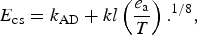 $$E_{{\rm cs}} = k_{{\rm AD}} + kl\left( {\displaystyle{{e_{\rm a}} \over T}} \right).^{1/8}, $$
where kl is a location-dependent coefficient given by manually selecting clear-sky hours from the dataset, e a is water vapour pressure (Pa) and k AD is an altitude-dependent coefficient for clear-sky emittance for a completely dry atmosphere following Marty and Philipona (Reference Marty and Philipona2000). Cloud cover varies between 0 (where E a = Ε cs) and 1 (E a = 1). The hourly values were then classified according to Petersen and others (Reference Petersen, Pellicciotti, Juszak, Carenzo and Brock2013) where C0 represents clear sky (0 ≤ n < 0.1), C1 represents low fractions of cloud (0.1 ≤ n < 0.4), C2 represents high fractions of cloud (0.4 ≤ n < 0.8) and C3 which is considered completely overcast (n ≥ 0.8). This classification was limited to the measurement of incoming longwave radiation at UWS, and as such does not account for the heterogeneous development of cloud across the glacier. However, the availability of incoming longwave radiation from CNR4 data at LWS and visual assessment of cloud from time-lapse cameras at both AWS generally support the classifications given by the above methodology.
Table 3. Description and value range for conditional classifications

4.2. Application of T a TGs in a distributed melt model
T a was distributed using gradients of air temperature, TG (°C m−1) given by regression against elevation or between station pairs as
 $${\rm TG} = \displaystyle{{T_{\rm a} 2 - T_{\rm a} 1} \over {Z2 - Z1}} = \displaystyle{{\delta T_{\rm a}} \over {\delta Z}},$$
where T a(n) defines the TT(n) air temperature record and Z(n) is the respective elevation of the stations. This investigation follows the convention whereby positive TGs indicate an increase in temperature with elevation. The ‘all-data’ T a distribution for this investigation utilises all on-glacier records of air temperature (except TT0) with a piecewise TG in elevation increments from 1844 to 2585 m a.s.l following Petersen and Pellicciotti (Reference Petersen and Pellicciotti2011). This all-data dataset (hereafter referred to as ADd) applies the TG between station pairs along the glacier (see Fig. 1) which varies with every time step. A TG between LWS and UWS data (AWSd) and the upper and lower most TT stations over debris (TT1–TT13d) were also employed for comparison. To account for the differences from melt model simulations (following section), distributed T a fields were further derived from:
-
(1) Temporally constant piecewise TGs, where all stations were employed (CNLd). This extrapolation method accounts for the spatial variability in T a for the full elevation range but keeps a constant TG between station pairs where the mean value of the whole season are used.
-
(2) Constant glacier-wide TGs where T a was extrapolated from single locations, LWS (a representative debris thickness of an on-glacier site) and off-glacier sites OG and nearby LB AWS. Constant linear TGs are those which either represents the average values calculated for Miage Glacier, the published value for debris-covered Baltoro Glacier (Mihalcea and others, Reference Mihalcea2006) or the commonly adopted ELR.
-
(3) The ADd dataset but with the inclusion of a temperature depression at sites within topographic troughs between the central/medial moraines (hereafter TRd). Trough areas were identified with three-dimensional visual interpretation from a 2010 LiDAR DEM and manually digitised in ArcGIS. T a was reduced within these areas using the TT7–TT8 regression equation.
-
(4) Constant TGs from individual stations as with (2) but where the strength of the constant value across the glacier was determined by the time of day (hourly average TG) or cloud factor (C0–C3). These extrapolation methods are hereafter referred to as z−c d, where z is the site of extrapolation and c is the condition classification (i.e. LWS-C d for T a forced from LWS by a cloud fraction TG).
All distribution methods are summarised in Table 4.
Table 4. Air temperature distribution methods for Miage glacier, 2014, with description of data (number of observations in parentheses) and the total range of lapse rate values for each method

* Identifies distribution methods that apply piece-wise lapse rates or where the lapse rate varies with each time step and thus the absolute max/min values are much larger. Lower weather station (LWS), OG and LB sites were the forcing locations for constant linear lapse rates.
4.3. Model approach
This investigation applies a modified version of the distributed debris-energy-balance (DEB) model developed by Fyffe and others (Reference Fyffe2014). The full details are therefore not repeated here, though the main components and key adjustments to the model are explored in this section.
The original model structure calculates sub-debris ablation rates across the glacier using the DEB model of Reid and Brock (Reference Reid and Brock2010). Key meteorological variables, including T a, wind speed and net radiation were distributed across the glacier and ablation (a) was calculated according to the surface cover type (debris, clean or dirty ice and snow) over a 30 m × 30 m cell area with an hourly time step
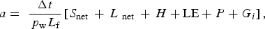 $$a = \; \displaystyle{{\Delta t} \over {\,p_{\rm w} L_{\rm f}}} \left[ {S_{{\rm net}} \, + \,L{\rm \;} _{{\rm net}} \, + \,H + {\rm LE} + P + G_i} \right],$$
where S net and L net are the respective net fluxes of shortwave and longwave radiation, H and LE are the turbulent fluxes of sensible and latent heat, and P is the heat flux provided by rain. These sources of energy were multiplied by the latent heat of fusion (L f) and the density of water (p w) for a given timestep (Δt). The conductive heat flux to the base of the debris (G i) was only calculated for debris surfaces and was calculated by DEB model based upon the temperature gradient through the debris layer (Reid and Brock, Reference Reid and Brock2010).
A grid of the glacier outline was digitised from 2009 DigitalGlobe satellite imagery in ArcGIS software including the Bionnassay, Tête Carrée and Dome glaciers as part of Miage Glacier. For calculation of melt, the Mont Blanc Glacier was excluded from the glacier outline as its tributary no longer forms part of Miage Glacier. Areas of dirty ice and patchy debris are based upon an assessment of satellite imagery and field observations within the transition zone at the tributary area, though in general, surface cover classifications differ only slightly from that proposed by Fyffe and others (Reference Fyffe2014). Areas of crevassing and large ice cliffs over the glacier were identified following Reid and Brock (Reference Reid and Brock2014), whereby slope angles were generated and digitised from a 2 m resolution 2010 LiDAR DEM and used as areas of increased surface roughness (from a value of 0.007–0.05 m, following Fyffe and others, Reference Fyffe2014), where the feature size was large enough to be accounted for in the cell resolution. Areas with multiple smaller crevasses were clustered under one digitised polygon for this reason.
The primary DEM for this model was derived from an airborne LiDAR survey in 2008, provided by the Regione Autonoma Valle d'Aosta. It has a higher spatial resolution of 10 m, which was resampled to a 30 m cell size and projected onto the WGS84 UTM 32N coordinate system. From this DEM a shading routine was incorporated to account for the calculation of diffuse radiation before the influence of cloud cover following the equation of Brock and Arnold (Reference Brock and Arnold2000). Binary grids were created utilising the hill shade algorithm in ArcGIS. Due to the small variations in shading between individual days, every day within a week was shaded with the hourly shading variations for the first day of that week. This was designed for computational efficiency of grid production and model input. For unshaded cells, proportions of direct and diffuse radiation were calculated using the slope and aspect of each cell and from solar zenith and azimuth angles for different hours of the day using a Sun position algorithm (Reda and Andreas, Reference Reda and Andreas2008).
Snow cover data were supplied at a 500 m resolution from MODISA1 for days where cloud cover was generally absent over the glacier area. Daily snow cover grids were produced by interpolating the snow cover data between cloud-free days. The Tête Carrée tributary and upper regions of the Dome and Bionnassay glaciers were assumed to be permanently snow covered based on satellite observations. Occurrence of snowfall events during the ablation season typically extended to elevations no lower than TT9 (2346 m) and were generally limited to the tributary area up glacier. Following Fyffe and others (Reference Fyffe2014), the model determines the values of emissivity, roughness and albedo based upon surface cover classification, whereby a snowmelt model is applied for 100% coverage of snow. For fractional snow cover, both the snowmelt model and the model of the surface type beneath are run with melt apportioned accordingly.
The distributed energy-balance model was run 19 times, with varying methods of T a estimation described in the previous section. Wind speed was assigned as a constant value from LWS and UWS for the respective lower and upper areas of the glacier, divided by the elevation of TT5 (2115 m), which was considered realistic given the topographically unconfined nature of the glacier at elevations lower than this site. For missing LWS data at the start of the season, all energy-balance equations were forced with data from the UWS. Due to topographical shading of UWS during hours of the morning (0700–0900) and evening (1800–20000), this gave a generally unrealistic value of shortwave radiation which was therefore calculated from the theoretical maximum transmittance through the atmosphere after attenuation due to Rayleigh scatter, aerosols and ozone following Pellicciotti and others (Reference Pellicciotti, Raschle, Huerlimann, Carenzo and Burlando2011) for July. Due to highly similar values at sites TT1, TT3 and OG and small data gaps for TT12, RH was extrapolated only from four, more spatially representative stations, TT1, TT5, UWS and TT10 and held constant above TT10. Surface RH was calculated from the Magnus–Tetens approximation using a dew-point temperature and radiative surface temperature from both AWS sites.
Debris thickness was estimated as a residual of the surface energy balance using surface temperatures derived from ASTER thermal imagery (Foster and others, Reference Foster, Brock, Cutler and Diotri2012). Given the greater thickness of the upper-glacier (above TT13) debris at the valley sides compared with that at TT9, the debris thickness in this model at elevations >2370 m (the highest measurement in Foster and others, Reference Foster, Brock, Cutler and Diotri2012) was given by simple nearest neighbour extrapolation in ArcGIS giving thickness values ranging from 2 to 6 cm.
5. RESULTS
5.1. Air temperature variations and meteorological controls
The 2014 Miage glacier ablation season was characterised by wet conditions and an average T a of 8.1°C across all station observations, with extremes of −3.0 and 24.1°C (Table 1). The distribution of T a was strongly related to elevation on the glacier with highly significant (p = 0.01) linear correlations for mean, maximum and minimum values as well as for the averages of the 10th and 90th percentiles (Fig. 4). The main exceptions to this are the low outliers at TT7 (thin debris) and TT12 (dirty ice) which reflect localised cooling associated with thin/patchy debris cover. The average localised TG (hereafter referred to as MG–TG) for Miage Glacier was found to be −0.0088°C m−1, similar to Koxkar debris-covered glacier, China (−0.0080°C m−1; Han and others, Reference Han2008; Juen and others, Reference Juen, Mayer, Lambrecht, Han and Liu2014) although for a shorter ablation period (May–September in Han and others, Reference Han2008).

Fig. 4. Mean (green), and upper (red) and lower (blue) 10th percentiles of T a for all TT stations and AWS (filled circles) against elevation on the Miage Glacier for the common observation period. TT7 and TT12 marked as anomalous means against elevation. Lines of best fit and slope coefficients are given for each data group.
Interestingly, the relation between T a and elevation is strong for all types of meteorological conditions (Fig. 5). TGs derived from the slope coefficients for all stations are more negative under clear skies compared with those under cloudy conditions, a difference between C0 and C3 of 0.0027°C m−1. Variations in wind speed and up/down-glacier flow at UWS had little impact on the strength of relationship with elevation, where a lower R 2 value for high wind speeds (0.89) was likely attributable to a small number of observations (120). Generally, low wind speeds tend to coincide with lower average T a and less negative (−0.0079°C m−1) TGs across the glacier. The scale of the TG increases with overall air temperature, but remains strongly related to elevation. The TT7 and TT12 anomalies are easily distinguishable for all conditions, particularly for C1 classifications (green circles in Fig. 5).

Fig. 5. Average T a (°C) against elevation (m a.s.l.) for different meteorological conditions described in Table 3. (a) Wind speed (m/s−1). (b) Cloud cover where C0 = clear sky, C1 = partly cloudy, C2 = mostly cloudy and C3 = overcast. (c) Wind direction. (d) T a percentiles (lower and upper 20th) for average of all stations. Meteorological variables (excluding T a) are measured only at UWS. Y-axes vary.
Figure 6 shows the comparison of hourly TGs in this study with the daily pattern between both AWS sites during the same period in 2006 from Brock and others (Reference Brock2010). TGs for 2014 were lowest overnight at ~−0.0070°C m−1, but increase sharply to −0.0100°C m−1 or more during daylight hours in response to insolation-driven heating of the debris, which leads to warmer T a. This warming effect was greatest on the lower glacier due to both thicker debris cover and less topographic shading compared with the upper glacier. The high number of station observations presented in this study reduces the strong increase in the late morning gradient from localised shading shown by the 2006 data.

Fig. 6. Hourly average 2014 (all data) and 2006 (LWS–UWS) Miage Glacier TGs (TG – °C m−1). 2006 data derived from Brock and others (Reference Brock2010). Horizontal lines show the averages for both years.
5.2. Air temperature estimation with TGs
Measured T a values were found to be estimated well by the linear TG between the lower (TT1) and uppermost (TT13) stations over debris (Fig. 7). The TT1–TT13 TG was found to overestimate at TT7 and TT12 sites, particularly during the night, and also to overestimate by up to 1°C during the daytime at TT11. The estimation of T a using the ELR is applicable to the lower glacier area at close proximity to LWS but at elevations greater than TT4/TT5, daytime values were significantly overestimated.

Fig. 7. Average hourly T a by station measured (red line) and estimated using a TG derived from the highest and lowest on-glacier stations over debris (green line) and from the LWS–ELR (blue line). Y-axis scale ranges vary.
Contrary to the typical overestimation of T a from off-glacier extrapolation for debris-free glaciers (e.g. Shea and Moore, Reference Shea and Moore2010), Miage Glacier demonstrates a general absence of the typical boundary layer cooling effect under positive ambient air temperatures, due to the warming effect of debris (Takeuchi and others, Reference Takeuchi, Kayastha, Naito, Kadota and Izumi2001). The on-glacier T a at LWS matches and even exceeds the off-glacier measurements at OG and LB. For the season average, T a at LWS was ~0.2°C warmer than OG (within the error range of the TT sensors); though up to 1°C warmer under cloudy conditions. Figure 8 demonstrates the extrapolation of the MG-TG (−0.0088°C m−1) from LWS, OG and LB for selected stations and while some variation in the estimated T a exists for the mid-morning, the choice of on-glacier/off-glacier forcing location results in little overall difference.

Fig. 8. On/OG forcing for T a at selected sites compared with measured average hourly values (red). R 2 values given for each forcing as a fit to the measured values.
5.3. Ablation measurements
Ablation for the 1 July–9 August period was generally greater than 9th August–27 September for most TT sites, with the exception of three of the up-glacier sites (Fig. 9a). This was partly due to absence of data for some stakes during the final part of the field season (green bars) and potential errors derived from short measurement periods (7 d) for all stakes at the beginning of August–September (Müller and Keeler, Reference Müller and Keeler1969; Munro, Reference Munro1989; Pellicciotti and others, Reference Pellicciotti2005). The beginning of this period was nevertheless characterised by a high number of intense rainfall events (daily total on 26th August of 41 mm, recorded at LB, equivalent to >16% of the season total) with greater than average wind speeds and slightly positive net longwave radiation. By comparison, the July–August period experienced the greatest frequency of clear sky conditions, the warmest average T a (8.5°C compared with 7.6°C for the latter period) and the most negative TGs. Thin debris sites at TT7 and TT9 and dirty ice site TT12 demonstrate the most rapid ablation. The relationship of mean ablation to debris thickness generally follows the established pattern of the declining limb of the Østrem curve (Østrem, Reference Østrem1959), although the increased ablation for very thin debris (‘effective thickness’) is not apparent for the stake measurements (Fig. 9b).

Fig. 9. (a) Ablation stake melt rates (m w.e. d−1) for combined periods and (b) the relationship with debris thickness (cm) at each site. Square boxes indicate the mean of each stake site and the total range for common observation period shown by the vertical error bars. Green bars in (a) indicate where stake melt out had occurred for the August–September period and therefore values are given only for a short (1 week) period in August. The July–August (August–September) period combines the former (latter) two subperiods of Table 2.
6. MODEL RESULTS
6.1. Model fit to ablation data
Figure 10 demonstrates the relationship between mean daily modelled and measured ablation (m w.e. d−1) for all stake locations for their respective measurement time periods. Results show a generally good fit of the model, with a RMSE of 0.0047 m w.e. d−1 for the ADd run without any model tuning (original parameters from Fyffe and others (Reference Fyffe2014)). Considering the daily averages, the model tends to underestimate ablation rates for thicker debris cover (larger circles) and overestimate for thinner debris and dirty ice.

Fig. 10. Measured vs modelled daily average ablation (m w.e. d−1) by stake where the circle size indicates the thickness of the debris cover and the error bars represent the total range of modelled ablation according to the various TG inputs as shown in Table 4. Error bars for measured ablation are not shown for visualisation purposes, though we consider a reasonable error margin of 0.05 m for the season total (~0.0005 m w.e. d−1).
In common with Fyffe and others (Reference Fyffe2014), variations in T a appear to have only a small effect upon modelled melt variability under thick debris cover. The variability in daily average ablation from different TGs (error bars) tends to increase with the magnitude of melt rate, in that thinner debris and higher elevation areas that melt faster are also more sensitive to T a (i.e. TT12 and TT9). Overestimates in melt typically occur more for higher elevation sites, where the effect of both thin debris and T a extrapolation from constant TGs become more pronounced. Forcing the energy-balance model with the LWS data and the standard TG (ELR) results in the greatest modelled melt errors (RMSE of 0.0058 m w.e. d−1).
6.2. Glacier-wide model output
In order to compare different T a model runs with ADd where data are available and not assumed, glacier-wide analysis of T a variations to model output are considered only at elevations <2600 m a.s.l. (~TT14). Results show that the glacier is generally insensitive to low magnitude temperature variations over debris cover (Fig. 11). The largest increase in modelled ablation relative to ADd is +4.3% for LWS-ELRd. Of greatest significance is that the application of the MG–TG extrapolated from LWS (LWS-MGd), results in an increase of <1% from the ADd run with similar performance as with TGs accounting for cloud cover effects (LWS-Cd). Overestimates of ablation are mostly attributable to debris-free model cells.
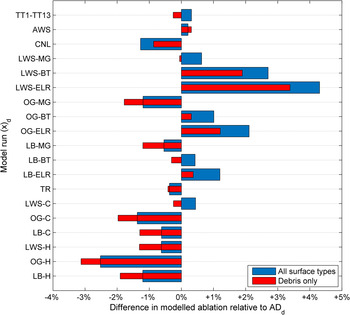
Fig. 11. Difference in glacier-wide ablation relative to ADd for all model runs (as shown in Table 4) expressed as a percentage. Blue (red) bars represent all surface types (debris only) below 2600 m.
Differences in calculated melt rates were dominated by the role of sensible heat fluxes and net longwave radiation. The total change in distributed values of these fluxes however was small when compared with ADd and were again only noteworthy for areas of thinner debris where temperature differences were larger between model runs (i.e. TT7). For example, maximum differences in sensible heat flux across the glacier between ADd and LWS-MGd were ~10 W m−2 for debris thicknesses of 2 cm. Further description of modelled differences is thus detailed only with regards to the calculated melt rate as a percentage relative to ADd.
The importance of applying a locally derived constant TG is apparent. Decreasing the TG from −0.0088 (Miage Glacier) to −0.0075°C m−1 (Baltoro Glacier – Mihalcea and others, Reference Mihalcea2006) increases total ablation for all surfaces by 2.1% when forced from LWS. Making the TG less negative from −0.0088 to −0.0065°C m−1 (ELR) results in a total increase of 3.7%. Extrapolating T a from OG sites results in a satisfactory model performance relative to ADd. Surprisingly, forcing air temperature from the OG site results in a decrease in modelled ablation of 1.8% (LWS/OG–MGd – Fig. 11) despite only a small disparity in average T a (~0.2°C). This is likely explained by the greater difference in on- and off- glacier temperatures during the daytime (Fig. 8), when melt rates were highest.
A piecewise application of constant temporal TGs (CNLd) was found to have little impact on the modelled ablation. Differences relative to ADd were found to be approximately −1%, and mostly the result of inversions in T a at TT7. Due to the strong dependency of T a on elevation for all hours of the day, temporally variable TGs were shown to be less relevant for modelling than in previous studies of debris-free glaciers (Petersen and Pellicciotti, Reference Petersen and Pellicciotti2011). Even the application of an hourly average TG for the season (Fig. 11) performed slightly worst than the assumption of the MG–TG forced from an on-glacier location (LWS-MGd), and all result in a decrease in modelled ablation relative to ADd, discussed in the following section. Forcing the model only with data from the two AWS (AWSd) or two TT stations (TT1–TT13d) resulted in little overall difference to the model.
Reduction of T a in topographic hollows for the TRd model run accounted for a total decrease in ablation of 0.37%. Thus, despite variations associated with locally thin debris being unaccounted for in the application of a constant TG, the overall impact on total melt from the glacier is small.
7. DISCUSSION
Data demonstrating that a locally derived, temporally constant and spatially homogenous TG (MG–TG) adequately accounts for the variations in T a across Miage Glacier contrasts with results for many debris-free glaciers (Gardner and others, Reference Gardner2009; Petersen and Pellicciotti, Reference Petersen and Pellicciotti2011; Petersen and others, Reference Petersen, Pellicciotti, Juszak, Carenzo and Brock2013; Ayala and others, Reference Ayala, Pellicciotti and Shea2015). The MG–TG is similar to that found for the debris-covered Koxkar Glacier (Han and others, Reference Han2008) and in a previous year for Miage Glacier (Brock and others, Reference Brock2010). The presence of a supraglacial debris layer that convectively heats the lower atmosphere through a flux of sensible heat and longwave radiation is a strong control on T a and is generally related to the thickness of the debris mantle (Brock and others, Reference Brock2010; Foster and others, Reference Foster, Brock, Cutler and Diotri2012). Miage Glacier has an inverse relation between elevation and debris thickness, particularly for the differences between the upper glacier (which is also topographically shaded during mid-morning and late evening) and thicknesses exceeding 1 m on the tongue. It is likely that the control of debris heating and its variance with elevation acts to reinforce the strong linear TG (MG–TG) found from regression with all on-glacier stations. Furthermore, this elevation dependency was found to be very strong and statistically significant when tested under different meteorological conditions (i.e. wind speed/cloud cover – Table 3). The TG was more negative for clear sky conditions when debris heating was maximised on the lower glacier compared with thinner debris at higher elevations. However, even under overcast (C3) conditions, when solar heating of the debris is suppressed, TGs still exceed that of the ELR and are comparable with those found for debris-covered Baltoro Glacier in the Karakoram (Mihalcea and others, Reference Mihalcea2006).
An interesting and somewhat counterintuitive finding for this work is the superior model performance of the MG-TG to a TG that varies as an hourly average (i.e. Fig. 6). It was found that although the hourly average TGs represent the average for the season, for days when overcast conditions dominated, application of a more negative daytime TG led to significant under-estimations in T a at higher elevations which were better modelled by the MG–TG. This result is in contrast to the findings for a debris-free glacier, where temporally variable TGs were considered important for accurately quantifying ablation (Petersen and Pellicciotti, Reference Petersen and Pellicciotti2011). Furthermore, forcing the MG–TG from LWS (LWS-MGd) in the model outperformed TGs dependent on an hourly cloud factor (Juszak and Pellicciotti, Reference Juszak and Pellicciotti2013; Petersen and others, Reference Petersen, Pellicciotti, Juszak, Carenzo and Brock2013). It is likely that the cloud factor poorly represents the variations of cloud development across the whole glacier during partly cloudy (C1) hours. It is possible that partly cloudy hours reflect warmer T a partly due to convective heating from the debris in preceding hours when shortwave radiation was direct, which may then act to skew the overall average TG of each cloud factor.
On-glacier T a was compared with two proximal off-glacier sites, revealing an absence of the glacier-boundary effect reported for debris-free ice surfaces (Greuell and Böhm, Reference Greuell and Böhm1998; Shea and Moore, Reference Shea and Moore2010). Previous work has found that over debris, katabatic wind is generally absent (Brock and others, Reference Brock2010), though to the authors knowledge, no studies have investigated this boundary layer effect in detail. On-glacier T a at LWS was found to exceed that of OG by ~0.2°C on average, and up to 1°C under cloudy conditions. The release of heat from debris is a likely cause of these differences for C3 conditions as the locations of LWS and OG are very similar (see Fig. 1). This finding may have important implications for future melt modelling studies over debris that utilise off-glacier station data.
Areas of thin debris cover experience more rapid rates of ablation (such as that measured at TT9 and TT12) and are also more sensitive to T a variations and the choice of temperature distribution method. Importantly, with the exclusion of ice cliffs, areas of thinner debris and exposed ice are evident only up-glacier, and as such forcing T a from on-glacier/OG locations near the glacier terminus results in more pronounced effects of constant TGs (i.e. TT12 – Fig. 7). Site selection for distributed energy-balance studies utilising only single on-glacier stations over debris may therefore be important and requires consideration of a representative glacier area. The choice of LWS as the on-glacier site for single station TGs was due to the debris thickness representing an approximate average for the glacier (Brock and others, Reference Brock2010; Foster and others, Reference Foster, Brock, Cutler and Diotri2012).
T a was found to be locally depressed over thin debris sites (i.e. TT7) due to removal of the insulating effect of thicker debris, a positive sensible heat flux (towards the surface) and lower longwave emission from the surface. Differences in low ablation beneath thick moraine debris (TT8) and high ablation under thin debris in ‘intermoraine’ troughs enhance the topographic variation and leads to cold air drainage into areas such as TT7 possibly as an extension of katabatic flow from debris-free up-glacier surfaces. These local temperature depressions are only found on the upper part of the debris-covered zone, as gravitational redistribution of debris quickly infills the valleys down glacier, eliminating both the local cooling effect and systematic topographic variation. However, incorporating these T a depressions into the model resulted in a maximum of 0.37% less total ablation relative to ADd. These effects appear very small compared with the overall ablation differences in this study, though they were parameterised only with the knowledge of T a at this one location and were modelled simply as a function of elevation using the regression relationship between TT8 and TT7 which is unlikely to fully account for the boundary layer processes at work. Furthermore, the effects of this potential cold air drainage could vary due to the scale of the topographic troughs and the increased fetch of the wind down glacier.
In general, it has been found that variation in T a has only a small effect on the overall modelled ablation as a result of the strong control of supraglacial debris thickness. Fyffe and others (Reference Fyffe2014) found a slightly greater sensitivity of Miage Glacier to artificial increases in T a, though accounted for the glacier tributaries including steep bare ice seracs (e.g. Mont Blanc Glacier) with high surface roughness values and thus large increases in calculated sensible heat flux. The sensitivity to T a was found here to be quite small in comparison with findings of model sensitivity to debris thermal conductivity and emissivity of Miage Glacier (Reid and Brock, Reference Reid and Brock2010).
A common approach is to model ablation using empirical temperature-index models that place greater emphasis on T a, even given the separation of a shortwave radiation term (Pellicciotti and others, Reference Pellicciotti2005). The work presented here demonstrates the suitability of a linear TG in deriving air temperature for a distributed energy-balance model of a debris-covered glacier and provides some analysis of why a linear TG is appropriate. Future work could benefit from testing the common assumptions found in this work with a more simplistic debris enhanced temperature-index model (Ragettli and others, Reference Ragettli2015).
8. CONCLUSIONS
Near-surface air temperature (T a) was monitored on the debris-covered Miage Glacier using a dense network of 19 stations over a period of 89 days in summer, 2014. Results from >31 000 hourly observations over a ~750 m elevation range reveal a strong, statistically significant relationship of T a with elevation under all meteorological conditions. In the absence of data, model studies for debris-free glaciers typically extrapolate T a from a single off-glacier station assuming a constant linear TG of −0.0065°C m−1 (Arnold and others, Reference Arnold, Rees, Hodson and Kohler2006; Nolin and others, Reference Nolin, Phillippe, Jefferson and Lewis2010), which has been shown to poorly account for the boundary layer effects over bare ice (Petersen and others, Reference Petersen, Pellicciotti, Juszak, Carenzo and Brock2013; Ayala and others, Reference Ayala, Pellicciotti and Shea2015). In contrast, this study finds that application of a locally derived, constant TG (MG–TG) over debris acts as a suitable estimation of T a. The MG–TG during the 2014 ablation season (−0.0088°C m−1) is found to match that for a previous year (Brock and others, Reference Brock2010) and at debris-covered glaciers in different parts of the world (Han and others, Reference Han2008), leading to the possibility of model transferability where meteorological data are available and knowledge of debris thickness is accounted for. Due to the convective heating over the debris surface, the application of the ELR is generally unsuitable for distributing T a to higher elevations where large overestimates occur, although produces only maximum differences of 4.3% compared with an all-data model run with piecewise extrapolation between all on-glacier stations. The absence of a distinct glacier-boundary layer effect over debris results in only a small difference between on-glacier and off-glacier T a forcing and thus we conclude that distributing T a from an off-glacier location is thought to be generally acceptable for debris-covered glaciers. For ice beneath thicker debris, sensitivity to T a variations is dampened and the effects of less negative TGs (ELR) are typically smaller. However, for areas of thin and patchy debris within the upper reaches of Miage Glacier (~TT9/TT12) where the effects of constant TGs are more pronounced and ablation is measurably more rapid, the sensitivity to T a in the model is greater. Considering the data intensive nature of this study, understanding the importance of T a within more simplistic empirical ablation models would be a suitable progression.
T a lower than that estimated by the MG–TG occurred at an ‘intermoraine’ valley site of thin debris cover, suggesting boundary layer cooling and possible cold air drainage may be locally important. Thus, while differences shown here are small and rather insignificant to the modelling of Miage glacier; the effect may be more significant at other sites with more extensive regions of ‘intermoraine’ debris. Considering the strong governance of debris thickness in a distributed energy-balance model, future work should emphasise the study of debris thickness variations and its evolution in time and space.
ACKNOWLEDGEMENTS
T. Shaw is the recipient of a Natural Environment Research Council (NERC) research studentship. We thank M. Vagliasindi and J.P. Fosson of Fondazione Montagna Sicura for logistical support at the field site and W. Smith and Northumbria University undergraduate students for assistance in setting up and taking down the stations. The air temperature data from the Lex Blanche station and the VDA DEM were kindly provided by Regione Autonoma Valle d'Aosta (Modello Altimetrico Digitale della Regione Autonoma Valle d'Aosta aut. n. 1156 del 28.08.2007). The airborne LiDAR data (2010 DEM) were provided by the NERC Airborne Research and Survey Facility (projects GB07–09 and GB07–10). We thank P. Deline for advice and extensive logistical support and I. Juszak for help with derivation of cloud factors. Finally, we thank scientific editor T. Mölg and two anonymous reviewers who helped to improve the quality of the manuscript.


 Open access