

1. Introduction
Knowledge of snow and ice surface melt rates is important for the correct assessment and management of water resources (Reference Hamlet and LettenmaierHamlet and Lettenmaier, 1999; Reference MarshMarsh 1999), including the prediction of seasonal or short-term discharge, for studies of glacier hydrology and dynamics (see Reference Fountain and WalderFountain and Walder (1998) and Reference WillisWillis (1995) for respective reviews) and of glacier mass balance (Reference Arnold, Willis, Sharp, Richards, Lawson and DevelopmentArnold and others, 1996; Reference RichardsRichards and others, 1996).
Surface melt rates can be calculated by means of two different approaches: physical energy-balance models and empirical temperature-index models. The former may be defined as a model in which each of the relevant energy fluxes at the glacier surface is computed from physically based calculations using direct measurements of the necessary meteorological variables, and the melt rate is calculated as the sum of the individual fluxes. The latter may be defined as a model in which the melt rate is calculated from an empirical formula in which air temperature is the sole measured input variable, although additional input variables, such as incoming shortwave radiation, may be incorporated through parameterizations based on time and location. Temperature-index models have been widely used for both glaciological and hydrological applications due to their parsimony in data requirement in comparison with the more sophisticated energy-balance models. However, their applicability is usually restricted to simulation of melt rates at daily or coarser resolution, and in a lumped or semilumped manner for calculation of average melt rates over a whole basin. Recently, an increasing need for high temporal and spatial resolution simulations of the melt rate (e.g. Reference HockHock, 2003) has prompted numerous attempts to combine the accuracy of physically based energy-balance models with the simplicity of temperature-index approaches.
The main aim of this study is to develop a melt model with lower data requirement than an energy-balance model but a stronger physical basis than current temperature-index models. This is achieved by:
-
1. incorporating variations in incoming radiation and albedo into melt calculations
-
2. developing a more physical representation of the surface energy balance in the model, through separation of temperature-dependent and temperature-independent energy sources.
Net shortwave solar radiation is the dominant source of melt energy on most glaciers (Reference Braithwaite and OlesenBraithwaite and Olesen, 1990; Reference BraithwaiteBraithwaite, 1995; Reference Arnold, Willis, Sharp, Richards, Lawson and DevelopmentArnold and others, 1996; Reference Greuell and SmeetsGreuell and Smeets, 2001; Reference Willis, Arnold and BrockWillis and others, 2002). Hence, in this investigation attention is focused on the energy input from shortwave radiation. In addition to incoming shortwave radiation, albedo is incorporated into the melt-rate calculation. Surface albedo is defined as the broadband, hemispherically averaged reflectance in the spectral range 0.3–2.8 µm, and is primarily controlled by the properties of the snow and ice surface. Albedo determines the amount of incoming shortwave radiation that is absorbed at the snow or ice surface, and thus exerts a strong influence upon the spatial and temporal evolution of melt rates. It is well known that albedo variations associated with snow metamorphism alone are a significant control on the surface melt rate, and in particular that summer snowfall events are of great importance to the summer energy balance (Reference Brock, Willis, Sharp and ArnoldBrock and others, 2000b). Indeed, the importance of taking into account albedo in melt computations through temperature- index models has been emphasized by Reference Lang and BraunLang and Braun (1990). Additionally, albedo variations on snow can be largely explained by temperature (Reference Brock, Willis and SharpBrock and others, 2000a) and may be parameterized purely as a function of temperature and/or age of the snow surface (US Army Corps of Engineers, 1956; Reference Brock, Willis, Sharp and ArnoldBrock and others, 2000b), and hence may be incorporated into a temperature-index model without the need for additional data.
A second aim of this paper is to assess the improvement in model performance associated with the inclusion of the shortwave radiation balance, independently of uncertainties introduced by parameterizations or extrapolation of the input variables. Thus, in a first stage the model is developed and tested at the point scale, where measured input variables can be used. Melt rates simulated by the temperature-index model are compared, for calibration and validation, to hourly ablation rates modelled by an energy-balance model, rather than measured melt rates, due to the relatively large errors associated with direct measurements of surface lowering over short time-scales. After the model is tested with measured input variables, its application with parameterized input is also evaluated.
An important aspect of this research is to test how temperature-index models cope with major changes in surface conditions during the ablation season, such as snow metamorphism and snow-to-ice transition. The inclusion of albedo is required to reflect the physical changes in glacier surface conditions that affect the surface melt rate over an ablation season. As yet, few studies have specifically examined the effect of the inclusion of albedo on the performance of a temperature-index model, or the enhanced temporal resolution and spatial transferability that might be achieved in this manner. Albedo was previously incorporated into a temperature-index melt model (Reference MartinecMartinec, 1989), but in that study albedo was prescribed based on the subjective evaluation of the surface state, and modelled melt rates were not validated. A model very similar to the one described in this paper was also developed by Reference Kane, Gieck and HinzmanKane and others (1997). That model, however, was applied not to an alpine glacier but to an arctic site characterized by a light snowpack (5–20 cm of water) and the presence of protruding vegetation;and daily, rather than hourly, melt-rate variations were examined. Therefore, the ablation season considered was much shorter than that of a glacier, and did not include variations in surface conditions such as the transition from snow to ice. Furthermore, in contrast to Reference Kane, Gieck and HinzmanKane and others (1997), our model is run with input data measured at the site of model application, thus avoiding errors introduced by their extrapolation in space.
Once the model performance is tested with measurements of the input variables, a third aim is to assess its performance using temperature data as the only measured input variable. Accordingly, the model is run using parameterizations of radiation and albedo which do not require more data than the simpler model versions used in this study. In this way, the model applicability is also established for operational purposes on glaciers where fewer data are measured.
This study uses a new dataset, collected on Haut Glacier d’Arolla, Switzerland, during the 2001 ablation season. Five automatic weather stations (AWSs) were operated on the glacier throughout the summer of 2001 to gain a better understanding of the spatial variability of melt rate. The enhanced temperature-index model and other versions of the temperature-index approach were developed at the central site on the glacier, and tested against hourly melt rates simulated by the energy-balance model at the four remaining locations distributed over the glacier.
2. Background
Temperature-index melt models are based on the assumption that melt rates are linearly related to air temperature, which is regarded as an integrated index of the total energy available for melt. The factor of proportionality is the so- called ‘degree-day factor’, DDF (mm °C–1 per time-step):

where M is the melt rate (mm w.e. per unit of time), T is the mean air temperature of each time-step at the screen level (°C) and T T is a threshold temperature above which melt is assumed to occur (e.g. 1 °C).
Attempts at relating melt rates to air temperature date back to the end of the 19th century (Reference Finsterwalder and SchunkFinsterwalder and Schunk, 1887) and since then this method has been widely applied for computing melt rates that are used as input for runoff models (Reference BergströmBergström, 1976; Reference TangbornTangborn, 1984; Reference Martinec and RangoMartinec and Rango, 1986), ice-dynamics models (e.g. Reference Huybrechts, Letréguilly and ReehHuybrechts and others, 1991; Reference OerlemansOerlemans and others, 1998) and studies of climatic sensitivity (Reference Laumann and ReehLaumann and Reeh, 1993; Reference Bøggild, Reeh and OerterBøggild and others, 1994; Reference Jöhannesson, Sigurdsson, Laumann and KennettJöhannesson and others, 1995; Reference JóhannessonJöhannesson, 1997; Reference Braithwaite and ZhangBraithwaite and Zhang, 1999). An extensive discussion of the temperature-index approach can be found in Reference HockHock (2003), together with an explanation of the accuracy achieved.
Despite their success in a wide range of lumped applications (see, e.g., Reference HockHock, 2003), temperature-index methods imply a strong simplification of complex physical processes which are more properly described by the energy balance of the glacier surface and overlying atmospheric surface layer. As a result, they suffer from two major limitations. First, their temporal resolution is restricted to daily or coarser resolution (Reference Kustas, Rango and UijlenhoetKustas and others, 1994), hence the approach is not appropriate for simulating the diurnal cycle of melt rate. Secondly, the spatial variation of melt rates across a glacier can only be simulated through changes in elevation associated with the air-temperature lapse rate. In reality, spatial melt-rate variations occur due to variations in the surface energy balance from location to location, and are controlled in a complex way by topographic features and surface conditions, principally surface roughness and albedo. Differences between snow and ice are often taken into account by specifying two different values of the degree-day factor for the two types of surface. This approach, which is appropriate for lumped calculations, is less suitable for distributed simulations of the spatial patterns of melt rate across a glacier.
Due to these limitations, some workers have attempted to incorporate additional meteorological variables and/or more physically based expressions in the standard temperature- index model (Equation (1)) (e.g. Reference Kustas, Rango and UijlenhoetKustas and others 1994; Reference Cazorzi and Dalla Fontana.Cazorzi and Dalla Fontana, 1996). This approach was developed further by Reference HockHock (1999), through the addition of a potential direct radiation term to the classic temperature- index model:

where M is the melt rate (mm h–1), T is hourly mean air temperature at the screen level (°C) and I POT is potential clear-sky direct solar radiation (Wm–2). MF and RF are two empirical coefficients, respectively the melt factor and radiation factor, which are expressed in mmh–1 °C–1 and m2 mm W–1 h–1 °C –1, respectively. The radiation factor has different values for snow and ice. Apart from temperature, no additional time-dependent meteorological variables are required, and values of/POT vary spatially according to the surface slope and aspect calculated from a digital elevation model (DEM). In addition to calculating topography- dependent melt-rate variations, hourly values of melt are computed, since I POT is calculated at an hourly time-step. Based on a comparison of bulk glacier discharge at Storglacia¨ren, Sweden, this method proved to be only slightly less accurate than a physically based distributed energy-balance model (Reference HockHock, 1999).
Despite the improvements afforded by Hock’s method, two limitations are still apparent. First, the variation in absorption/reflection of radiation at the surface, i.e. albedo, is dealt with crudely, with only two different RF values, for snow and ice, used. Second, according to Equation (2), the MF and RFI POT are lumped together and multiplied by temperature, whereas, from a consideration of the energy balance, it is apparent that RFI POT should be independent of temperature. Hock’s model attempts to improve the simple temperature-index method by varying the degree-day factor in space and time as a function of a potential radiation term dependent only on topography and solar geometry, and therefore in a way that is compatible with the data requirements of a simple temperature-index model. In this respect, the improvement obtained over a simple temperature-index model is remarkable. However, when shortwave radiation data are available, a more physical representation of melt, based on the energy-balance equation (Reference Greuell, Genthon, Bamber and PayneGreuell and Genthon, 2003), seems more appropriate to the formulation of the model.
3. Measurements
3.1. The study area
The model was developed and tested using measurements made during the 2001 summer season on Haut Glacier d’Arolla. The glacier is situated at the head of the Val d’Hérens, in Valais, Switzerland, and is about 4 km long, has an area of about 6.3 km2 and ranges in elevation from 2550 to >3500 m. It consists of an upper basin with northwesterly aspect feeding a northward-flowing glacier tongue (Fig. 1).

Fig. 1. Map of Haut Glacier ďArolla, showing the location of the five AWSs used in the study and of the permanent station in the proglacial valley. The image shows the DEM of Haut Glacier d’Arolla and the surrounding area, as derived by digital photo- grammetry using aerial photographs taken in September 1999. Grid size is 10 m. The image was relief shaded. The black line indicates the glacier border.
The glacier has been the site of an integrated study of meteorology, hydrology, water quality and ice dynamics for >10 years (Reference RichardsRichards and others, 1996), and numerous datasets and energy-balance models for the glacier exist. In particular, two surface energy-balance models were developed and tested using data collected on the glacier, namely those described by Reference Arnold, Willis, Sharp, Richards, Lawson and DevelopmentArnold and others (1996) and by Reference Brock and ArnoldBrock and Arnold (2000). The latter is used in this paper to calculate reference surface melt rates.
3.2. Meteorological measurements and measurements of surface lowering (ablation)
Meteorological input data are needed for both the enhanced temperature-index model described in this paper and the energy-balance model. Five AWSs were established during summer 2001 along two intersecting transects on Haut Glacier d’Arolla (Table 1). The location of the five weather stations is shown in Figure 1. The north-central, central and south-central stations were set up along a transect at about 2920ma.s.l., to observe cross-glacier changes in the meteorological variables independently of elevation. The second transect was formed by the lowest, central and uppermost stations, placed at 2830, 2920 and 3015ma.s.l. respectively. Combination of the two transects provides a picture of the spatial variability of melt rates and driving meteorological variables associated with along- and across- glacier changes in topography and surface conditions (Reference Strasser, Corripio, Pellicciotti, Burlando, Brock and FunkStrasser and others, 2004).
Table 1. Characteristics of the locations of the five AWSs

During the 2001 ablation season, the central, north- central and lowest stations were located in the ablation area, whereas the uppermost and south-central stations were in the accumulation area of the glacier. The characteristics of the five stations are listed in Table 1. Northerly aspect and shading (Fig. 1; Table 1) lead to the survival of the winter snowpack at the south-central station, while ice at the same elevation became exposed at the central and north-central stations by mid-August. All weather stations were surveyed daily during the period 16–29 May and again in the period 16 July–15 August. Three of the five stations did not work for short intervals in the middle of the melt season (Table 1).
At each station, the following meteorological variables were recorded: air temperature (°C), relative humidity (%), wind speed (ms–1) and direction (°), incoming and reflected shortwave radiation (W m–2). At the central station, net radiation (W m–2) was also monitored. Measurements were taken every 5s and the average stored every 5 min on Campbell CR10 and CR10X dataloggers. The sensors were mounted on stations made up of a tripod and an arm, on which the sensors were fixed 2 m from the bottom. A square metal plate of 30 × 30 cm was fixed at the end of each leg, so that the station was sitting on the snow or ice surface and could sink together with the melting surface to maintain a constant distance between the sensors and the surface. This also ensured that surface fluxes were measured in a surface- parallel plane (Reference MannsteinMannstein, 1985; Reference Brock, Willis, Sharp and ArnoldBrock and others, 2000b; Reference Greuell, Genthon, Bamber and PayneGreuell and Genthon, 2003). This was not always the case, however, since stations initially sank in the snowpack for about 0.2–0.3 m until they reached equilibrium. Thus, the heights of the wind, temperature, humidity and radiation sensors were nominal. The temperature and humidity sensors were shielded and artificially ventilated. The raw data were aggregated to hourly averages, and these hourly datasets constituted the input to all the melt models.
Additional meteorological data were provided by an AWS located at a proglacial site approximately 1 km from the glacier terminus, which has operated since November 2000 (Fig. 1). The proglacial station records the same variables as the glacier central station and, in addition, solid and liquid precipitation.
At the location of the central station, an ultrasonic ranger was installed between 29 May and 14 August, in order to measure continuously the lowering of the glacier surface. The ultrasonic ranger measured every 5 s, and data were stored every 5 min on a Campbell CR10X datalogger. At the location of the central and uppermost stations, ablation stakes were also installed, as part of a set of 20 stakes that were installed widely across the glacier. Density measurements were made during the installation of the stakes and the ultrasonic ranger, and later on at various intervals, to enable the conversion of surface lowering into snow water equivalent (w.e.) melt.
3.3. Melt calculations using the energy-balance model
Time series of hourly melt rates are required both in the optimization of model parameters and in the testing of model performance. Direct measurements of surface lowering at ablation stakes suffer from significant errors at time periods less than 1 week (e.g. Reference Müller and KeelerMüller and Keeler, 1969; Reference MunroMunro, 1990), while both direct measurements at ablation stakes and continuous monitoring of surface lowering from ultrasonic rangers are affected by time lags between melt and its expression as a lowering of the surface (Reference MunroMunro, 1990). For these reasons, an energy-balance model was used to compute hourly melt rates at each of the locations of the five weather stations. The model is described in detail in Reference Brock and ArnoldBrock and Arnold (2000).
When incoming and reflected shortwave radiation fluxes are measured directly (as at each of the AWSs), energy- balance theory enables point melt rates to be calculated, with a very small margin of error, from accurate local meteorological measurements (e.g. Reference Brock, Willis, Sharp and ArnoldBrock and others, 2000b; Reference Willis, Arnold and BrockWillis and others, 2002). Thus, for the AWS sites, the energy-balance model should provide a reliable reference melt rate. Most significantly for this study, the energy- balance model calculates real-time melt values, unaffected by time lags between melting and surface lowering.
The Reference Brock and ArnoldBrock and Arnold (2000) model computes the surface energy balance and surface melt rate for a point on a melting snow or ice surface, and assumes that there is no conduction of heat into the snowpack or glacier. Normally, incoming shortwave radiation and albedo are required inputs to the model. The model was adapted for this study to accommodate the availability of direct measurements of both incoming and reflected shortwave radiation at each AWS. The adapted model is forced by the following hourly measurements of meteorological variables: incoming shortwave radiation (Wm–2), reflected shortwave radiation (Wm–2), air temperature (°C), air vapour pressure (Pa) and wind speed (ms–1). Direct measurement of both incoming and reflected shortwave radiation fluxes ensures that a major source of error in energy-balance models, due to the uncertainty in the surface albedo value, is avoided.
The sensible and latent fluxes are evaluated by means of the ‘bulk’ aerodynamic approach, using the Monin–Obukhov similarity equations to account for stable conditions in the glacier surface boundary layer (Reference Ambach and KirchlechnerAmbach and Kirchlechner, 1986; Reference OkeOke, 1987; Reference MunroMunro, 1989, Reference Munro1990). This method requires wind speed, temperature and humidity to be measured at only one height above the surface. The scaling lengths for temperature and humidity (zt and ze, respectively) are computed as functions of the surface aerodynamic roughness length (z0) and flow, using the roughness Reynolds number, following Reference AndreasAndreas (1987) (see Reference Brock and ArnoldBrock and Arnold (2000) for an extensive discussion on this point). Although some of the assumptions of bulk transfer theory are not met over melting glacier surfaces, due to the presence of a low-level wind-speed maximum, recent field and modelling studies have shown this method introduces only a small error into turbulent flux calculations (Reference MunroMunro, 1990; Reference Denby and GreuellDenby and Greuell, 2000). Furthermore, the turbulent fluxes make a relatively minor contribution to total surface melt at Haut Glacier d’Arolla (Reference Arnold, Willis, Sharp, Richards, Lawson and DevelopmentArnold and others, 1996).
The model also requires that the z0 for the location is specified. As no z0 measurements were made in this study, a simple scheme for z0 was employed, based on field observations, analysis of photographic records and of the timing of snowfalls, where z0 = 0.1 mm following snowfall, and z0 = 1.0mm after snowfall when melting has taken place, and on ice. This scheme is based on a recent study of surface roughness on Haut Glacier d’Arolla (Reference BrockBrock, 1997). An order-of-magnitude error in z0 leads to a 25% error in the turbulent heat fluxes (Reference Denby and GreuellDenby and Greuell, 2000), so errors in the turbulent heat flux calculations due to uncertainties in the value of z0 should be well below this level.
The outgoing longwave radiation flux is computed assuming that the surface is at 0°C and radiates as a black body. Incoming longwave radiation is also calculated from the Stefan–Boltzmann relationship, where the effective emissivity of the sky is computed as a function of cloud cover which in turn is estimated from the ratio of measured incoming shortwave radiation to potential clear-sky incoming shortwave radiation (for full details see Reference Brock and ArnoldBrock and Arnold, 2000).
Figure 2 shows hourly melt rates computed by the energy- balance model at the central station for the entire ablation season. It depicts the typical pattern of ablation rates over the course of a melt season, which was similar at all stations. Melt rate is lower at the start of the season due to the high snow albedo and lower temperature, and increases over the course of the ablation season with increasing temperature and decreasing albedo. There are marked diurnal cycles ranging from 0 to a maximum of ~5–9mmw.e.h–1 during the day. Such diurnal cycles are dominated by the pattern of incoming shortwave radiation and therefore tend to peak in the early afternoon.

Fig. 2. Reference hourly melt rates computed by the energy-balance model at the central station for the full melt season, together with measured air temperature (black trace) and albedo (red trace) at the same station (top). Albedo is plotted only for the daytime hours (measured incoming shortwave radiation above 50Wm–2), hence the discontinuous line.
To validate the energy-balance model, melt computed with the model at the central station was compared to both the ultrasonic ranger readings and surface lowering recorded at the ablation stake. For comparison, the period 23 July–14 August was selected, because of the availability of a reliable snow density (p) measurement. The ultrasonic readings were smoothed to remove noise using a Hamming window, and both the ultrasonic and stake readings were converted into w.e. by using the density measurement taken on 5 August (ρ = 504kgm–3). Ablation stake readings were made on 23 and 26 July and 2, 5, 10 and 12 August.
Figure 3 shows the comparison of the simulated cumulated hourly melt with the ultrasonic range series and the discrete stake readings. The energy-balance simulations and the measurements are generally in very good agreement, apart from the last few days of the period (11–14 August), immediately before the transition from snow to ice occurred at this site, when the energy-balance melt slightly overestimates the melt measured by the ultrasonic ranger, but is still in very close agreement with the final ablation-stake measurement on 12 August. These results demonstrate that the energy-balance simulations can be confidently used as the reference melt rate.

Fig. 3. Comparison between melt simulated by the energy-balance model, measured at the ultrasonic gauge, and readings at the ablation stake, at the central site, for the period 27 July–14 August.
4. Development and Testing of the New Temperature-Index Model
4.1. Description and formulation
The temperature-index model proposed here computes melt as the sum of two components:

where α is albedo and G is incoming shortwave radiation (Wm–2). TF and SRF are two empirical coefficients, respectively the temperature factor and shortwave radiation factor, expressed in mmh–1 °C–1 and m2mmW–1h–1. TT is equal to 1 °C. When temperature is below TT no melt occurs.
The model assumes that daily albedo data are appropriate, whereas all the other variables are used at hourly resolution. Although albedo is known to increase with increasing solar zenith angle (θ), this effect is greatest at high θ, and it is generally accepted that а is largely independent of θ when θ <50° (Reference Wiscombe and WarrenWiscombe and Warren, 1980; Reference Konzelmann and OhmuraKonzelmann and Ohmura, 1995; Reference Brock, Willis and SharpBrock and others, 2000a). Hence, one daily albedo value was used, based on albedo measured for small θ, when incoming shortwave radiation is greatest. Albedo is also known to increase with cloud cover (Reference Cutler and MunroCutler and Munro, 1996; Reference BrockBrock, 2004);however, consideration of cloud-cover variation is beyond the scope of our model comparison study.
In Equation (3), the contributions to melt energy of the longwave radiation and turbulent fluxes in one term and shortwave radiation in the other are clearly separated. In order to test whether the separation of temperature-dependent and temperature-independent energy sources improves the calculation of melt rates, an alternative formulation (incorporating α) was implemented and tested, based on the multiplicative formula of Reference HockHock (1999), and compared with the more physically based Equation (3):
Note that in Equation (4) the empirical coefficient SRF has different dimensions than in Equation (3), as it is expressed in m2 mm W–1 h–1 °C–1.
To test the model applicability to glaciers with more limited data availability than in this study, model D was also run using modelled radiation input data. This also allows a comparison between models with the same measured input data. Incoming shortwave radiation was modelled using a parametric model for clear-sky conditions based on Reference IqbalIqbal (1983) and modified by Reference CorripioCorripio (2003). The model computes absorption, reflection and transmission of solar irradiance through the atmospheric path between the top of the atmosphere and the glacier surface. It also takes into account the effect of topography on the radiation receipt. A new set of algorithms (Reference CorripioCorripio, 2003) was used to calculate terrain parameters such as slope gradient and aspect from a DEM of the glacier, and employed in the actual solar radiation model to compute the exact position of the sun, the angle of incidence of the sun on the surface, the hill shading and the sky- view factor. The DEM of the glacier, with 10 m resolution, was produced from aerial photographs taken in 1999.
The model can compute clear-sky incoming shortwave radiation with high accuracy, but omits cloud cover. Treatment of cloud effects is important, because cloud cover plays a crucial role in reducing the total amount of incoming shortwave radiation reaching the ground (e.g. Reference Dai, Trenberth and KarlDai and others, 1999; Reference HockHock, 1999). On Haut Glacier d’Arolla, clouds reduced the incoming shortwave radiation at the top of the atmosphere by about 30% during the 2001 ablation season (Reference Strasser, Corripio, Pellicciotti, Burlando, Brock and FunkStrasser and others, 2004). Consequently a cloud- cover parameterization was developed in this study, based on the diurnal range of air temperature, which has been shown to be one of the best indicators of cloud cover in a number of studies (e.g. Reference Dai, Trenberth and KarlDai and others, 1999). First, ‘cloud factors’, defined as the ratio of measured to modelled clear- sky incoming shortwave radiation (Reference Greuell, Knap and SmeetsGreuell and others, 1997), were computed at each station. Cloud factors vary from 1.0 when there is no cloud cover (measured radiation = modelled clear-sky radiation) to 0.0, a theoretical minimum when all incoming radiation is obscured by cloud. Daily cloud factors were derived as a weighted mean of hourly cloud factors, the hourly weighting being the ratio of the modelled clear-sky incoming shortwave radiation in that hour to the daily total modelled clear-sky incoming shortwave radiation. Hence, the daily cloud factor is weighted to the middle part of the day, when any incidence of cloud cover has a relatively large impact on the incoming shortwave radiation. The daily cloud factors were then regressed against the daily temperature range computed at the stations both on the glacier and at the permanent station in the proglacial valley. Daily cloud factors varied little between the five stations, so a constant value was used for the entire glacier. Temperature range measured on the glacier was found to be a poor indicator of cloud factors. This is due to the narrow daily temperature range in the glacier surface layer (Reference Greuell and Böhm.Greuell and Böhm, 1998). Hence, daily temperature range at the proglacial weather station was used to predict daily cloud factors on the glacier. A linear regression relationship gave the best fit. Figure 4 shows the scatter plot of daily cloud factor at the central station against daily temperature range computed at the permanent station outside the glacier, together with the linear regression used. There is large scatter in the relationship. This is partly due to the fact that temperature variations alone cannot entirely explain variations in the cloud cover and to the use of temperature variations recorded outside the glacier, which also respond to cloud-cover variations outside the glacier. However, to test the potential of application of the enhanced model to glaciers where only temperature data are available, this parameterization was used in this study, and daily cloud factors were applied to reduce the clear-sky modelled radiation simulated with the solar radiation model described above.

Fig. 4. Daily cloud factor at the central station vs daily temperature range at the permanent station in the proglacial valley (see Fig. 1).
Snow albedo was computed using the Reference Brock, Willis and SharpBrock and others (2000a) parameterization for deep snow. This parameterization was chosen because it relies solely on temperature data, together with the timing of snowfalls, as input to the model. Therefore, it is compatible with use in a temperature-index model. In addition, it was developed and tested using an extensive dataset of spatially distributed albedo measurements on Haut Glacier d’Arolla. Daily snow albedo as is computed as a logarithmic function of accumulated daily maximum positive temperature since snowfall:
where T a is accumulated daily maximum temperature >0°C since snowfall (°C), and p 1 and p 2 are empirical coefficients, where p1 is the albedo of fresh snow (for T a¼1 °C).
The parameterization was recalibrated using the data measured at the central station in the 2001 ablation season. Albedo of ice was assumed to be constant and equal to the mean ice albedo measured at each station.
4.2. Calibration and validation
Hourly melt rates calculated with the energy-balance melt model were used to calibrate and validate the temperature- index models. In the process, a comparison was made of the performance of four different levels of temperature-index model: the ‘classical’ temperature-index model using temperature only (Equation (1); model A hereafter); Reference HockHock’s (1999) model (Equation (2); model B hereafter), which uses temperature and parameterized potential direct solar radiation as input;an enhanced temperature-index model including incoming shortwave radiation and albedo in a multiplicative form (Equation (4); model C hereafter);and the enhanced temperature-index model including incoming shortwave radiation and albedo in an additive form (Equation (3); model D hereafter). The four corresponding formulations used in this study are listed in Table 2. Where, in later sections, model D is forced by modelled input variables it will be referred to as model E.
Table 2. Form of the different levels of temperature-index models used in the study, and parameter values obtained with the calibration at the central station. M is melt rate, T is mean air temperature, I POT is potential clear-sky direct solar radiation, G is global radiation and α is albedo

To assess the performance of the different model versions, the efficiency criterion R 2 (Reference Nash and SutcliffeNash and Sutcliffe, 1970) was employed, defined as:

where M is hourly melt rate and the subscripts r and s refer to the reference and simulated melt rate, respectively. The bar refers to the mean, and n is the number of time-steps for which R 2 is calculated. The criterion has been used for evaluation of model performance in a wide range of hydrological studies (e.g. Reference Wilcox, Rawls, Brakensiek and WrightWilcox and others 1990) and more recently in glaciological applications (Reference HockHock, 1999; Reference Klok, Jasper, Roelofsma, Gurtz and BadouxKlok and others, 2001; Reference Zappa, Pos, Strasser, Warmerdam and GurtzZappa and others, 2003).
4.2.1. Model calibration
Parameter values for each model were optimized at the central station using meteorological data and the computed hourly energy-balance melt rates for the entire melt season, from 30 May to 12 September 2001 (with a gap of 11 days in July;Table 1). The site was snow-covered from 30 May to 20 August and then ice was exposed from 20 to 31 August, when a heavy snowfall occurred. For model A, the degree- day factor was calibrated separately for snow and ice. Both factors were allowed to vary over a wide range of values, and the factors associated with the highest R 2 were chosen. Model B has three coefficients, as the radiation factor RF has different values for snow and ice. They were optimized by trying all possible combinations of the three parameters and choosing the one corresponding to the highest R2. For models C and D, which employ two coefficients, all possible combinations of the two coefficients were tried, and the combination that maximized the efficiency criterion was adopted. Model E uses the same coefficients as model D, so that the reduction in the model’s performance associated with using parameterized input data can be assessed. Furthermore, since the model D SRF value was optimized using measured input it should be transferable from one study to another.
4.2.2. Model validation
The four levels of temperature-index model were independently validated at the locations of the four other weather stations. Using the coefficients obtained from the parameter optimization at the central site, the models were run at each of the remaining weather stations for the full melt season, and the predicted hourly melt rates were compared to the melt rates calculated by the physically based energy-balance model. Separate calibration and validation datasets ensure that the comparison of the different levels of temperature-index model is impartial.
5. Results
5.1. Model calibration
Table 2 shows the optimal model parameters for the four different models, and the corresponding efficiency criteria R 2. The optimum degree-day factor for the simple temperature-index model is 0.32 mm h–1 °C–1 for snow and 0.45 mm h–1 °C–1 for ice. These values are in agreement with those reported in the literature (Reference BraithwaiteBraithwaite, 1995; Reference HockHock, 1998). Inclusion of shortwave radiation improves the model performance considerably, as shown by the higher R 2 values of models B–D (Table 3, column 1), and already demonstrated by numerous authors (e.g. Reference Kustas, Rango and UijlenhoetKustas and others, 1994; Reference HockHock, 1999). The R 2 value increases from model B to C to D. Inclusion of albedo alone leads to an improvement in model performance from R2 ¼ 0.769 (model B) to R 2 ¼ 0.866 (model C). The R 2 of model D is 0.911 and is the highest overall. The improvement in performance from model C (R 2 ¼ 0.866) to model D (R 2 ¼ 0.911) is entirely due to the separation of temperature-dependent and temperature-independent terms.
Table 3. Efficiency criterion R 2 for the calibration site (central station) and for the four validation sites

Figure 5 shows the effect of variations (10% incremental variations) in TF and SRF of model D around their optimal values on model performance. It can be seen that the model is sensitive to the value of SRF but much less so to TF.

Fig. 5. Model D sensitivity to TF (top) and SRF (bottom).
5.2. Model validation
The values of the efficiency criterion R2 computed at the validation sites for the four levels of model are listed in Table 3. Comparison of models at any location shows that model performance improves with increasing sophistication of the model (i.e. from model A to D) at all four sites. The R2of model D ranges from 0.895 (south-central station) to 0.955 (lowest station). Model D melt shows good agreement with the reference melt rate over the entire period (Fig. 6), although the model tends to slightly overestimate low melt rates and underestimate high melt rates.

Fig. 6. Model D hourly melt rate vs reference melt rate computed by the energy-balance model at the four validation sites.
In general, the enhanced model accounts for 90% or more of the variation in melt rate calculated by the energy- balance model (Table 3). Figure 7 provides a visual assessment of the improvement in model performance that is obtained from model A to D, at one of the validation sites, the uppermost station. Model A clearly does not reflect the diurnal melt variations, and in particular underestimates the high melt rates during the day.

Fig. 7. Model A, B, C and D hourly melt rate vs reference melt rate computed by the energy-balance model at the uppermost station.
Hourly melt rates computed at the lowest station by the four temperature-index models, together with the reference melt rate calculated by the energy-balance model, for the periods 21–28 July and 10–15 August are shown in Figure 8. At this site, from 2 August onwards, a gradual transition from a surface with higher albedo (continuous snowpack) to one with lower albedo (thin, patchy snow cover) occurs, until bare ice was exposed on 10 August. In response to the decrease in albedo, the reference melt rate almost doubles with the transition from a snow (21–28 July) to an ice (10–15 August) surface (Fig. 8). On snow (21–28 July), model D performs better than the other models, closely matching the reference melt rate. Models B and C also have peak melt rates similar to the energy-balance calculations, but with small underestimations (23, 25 and 26 July).

Fig. 8. Hourly melt rate simulated by the four temperature-index models vs the reference melt rate computed by the energy-balance model, 21–28 July and 10–15 August (tick mark labels at 1200h on each day) at the lowest station. Measured hourly albedo is also shown (top trace). At this site, ice becomes exposed on 10 August.
Conversely, marked differences between models B, C and D are observed after the transition to ice. The reference melt rate over the period 10–15 August is matched very closely by model D, and fairly closely by model C, both of which include albedo, but not by model B (Fig. 8). The tendency for models B and C to underestimate ice surface melt rates is repeated at all the stations in the ablation zone. The underestimation does not occur every day on ice, however, due to the influence of temperature variations, so that on days of high air temperature (e.g. 14 and 15 August) peak reference melt rates are matched closely, or even exceeded, by model B and C melt rates (Fig. 8).
Figures 9 and 10 show comparison of modelled and reference hourly melt rates during the period 20–27 June at the south-central station and 31 July–7 August at the lowest station, respectively. It can be seen that on a warm day (26 June) models B and C considerably overestimate the reference melt rate, whereas on a cold day with high incoming radiation (5 August) both models considerably underestimate melt. On both of these days the melt rate simulated by model D agrees very well with the reference melt. Similar fluctuations in melt rate, simulated by models B and C and associated with fluctuations of the air temperature, were observed at all validation sites throughout the season.

Fig. 9. South-central station. Temperature (above) and hourly melt rate simulated by the four temperature-index models vs the reference melt rate computed by the energy-balance model, 20–27 June (tick mark labels at 1200 h on each day).

Fig. 10. Lowest station. Temperature (above) and hourly melt rate simulated by the four temperature-index models vs the reference melt rate computed by the energy-balance model, 31 July–7 August (tick mark labels at 1200 h on each day).
Comparison between the efficiency criteria R 2 of model D at the four validation sites shows that the R 2 is highest at the north-central and lowest stations (Table 3). At these stations, the efficiency criterion of model D is even greater than the calibration R 2 at the central station (Table 3). Both sites were located in the ablation area of the glacier (Fig. 1), where albedo variability is the highest (Table 4).
Table 4. Albedo statistics at the five AWSs
5.3. Enhanced model with parameterized data
Modelled clear-sky incoming shortwave radiation at the central station for the period 9–18 June is shown in Figure 11, together with measured incoming shortwave radiation and daily cloud factor. It can be seen that the agreement between clear-sky modelled radiation and measured incoming shortwave radiation is very good for clear-sky conditions (on 12 and 14 June). When the effect of clouds is considered, the modelled radiation is generally underestimated, in particular on cloud-free days (e.g. 14 and 15 June). This was repeated at all stations. The incoming shortwave radiation is generally fairly well reproduced under overcast conditions (e.g. on 10 and 11 June;Fig. 11), but these are also the conditions where the energy input from the shortwave radiation balance is low. As the cloud factors have daily resolution, this method cannot reproduce the sub-daily variations observed in the measured incoming radiation, as on 13 and 18 June.

Fig. 11. Daily cloud factors, measured and modelled incoming shortwave radiation at the central station, including the effect of cloud factor, 9–18 June.
Figure 12 shows measured and modelled daily albedo at the validation sites. The agreement between modelled and measured albedo at the south-central station is good (Fig. 12b), whereas more discrepancies can be observed at the uppermost station (Fig. 12a). These errors are not really due to the albedo parameterization itself but due to the incorrect identification of the timing and volume of fresh snowfall events. This is a common problem in glacier melt modelling due to the need to extrapolate rainfall events recorded at a proglacial station to the glacier based on a temperature lapse rate, and, for albedo simulation, the correct identification of the elevation on the glacier of the rainfall-to-snowfall transition is critical. For an extensive discussion on the application of this albedo parameterization at the five station sites, see Reference PellicciottiPellicciotti (2004).
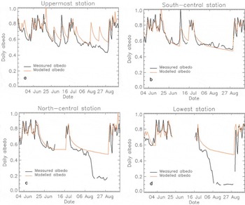
Fig. 12. Measured and modelled daily albedo at the uppermost, simulated using the Reference Brock, Willis and SharpBrock and others (2000a) parameterization.
The R 2 of model E at each site is lower than those of model D (Table 3), due to a tendency to underestimate reference melt rates (Figs 8–10). Compared with model B, which has the same data requirements, it can be seen that model E performs better for all sites except the south-central station (Table 3). The most significant improvement is at the north-central and lowest stations in the ablation zone, which have the highest albedo variability (Table 4). The relatively poor performance of model E (and D) at the south-central station is discussed in the next section.
6. Discussion
6.1. Enhanced model with measured input variables
From analysis of melt rates simulated by the four models in comparison with energy-balance calculations, as depicted in Figures 8–10, it is clear that two main characteristics of the enhanced model explain why it performs better than models A–C:
-
1. Through the inclusion of albedo in the shortwave radiation term, the enhanced temperature-index model can calculate the changes in melt rate associated with snow metamorphism (all sites) and with the transition from snow to ice (ablation area sites).
-
2. Through separation of temperature-dependent and temperature-independent energy sources, the over-sensitivity of the calculated melt rate to temperature extremes, symptomatic of more empirical melt models, is considerably reduced in the new model.
Inclusion of albedo eliminates the need to adjust the melt factor over the ablation season. The dependence of the degree-day factor on albedo has previously been established (Reference BraithwaiteBraithwaite, 1995; Reference Arendt, Sharp, Tranter, Armstrong, Brun, Jones, Sharp and WilliamsArendt and Sharp, 1999). Traditionally, temperature-index models overcome the problem of changing surface properties using different parameter values calibrated separately for snow and ice (Reference BraithwaiteBraithwaite, 1995; Reference Schreider, Whetton, Jakeman and PittockSchreider and others, 1997; Reference HockHock, 1999). This approach, however, has a weaker physical basis than model D and is unable to account for melt-rate variations resulting from albedo variations on a single surface type (e.g. the decay of albedo following a fresh snowfall). Furthermore, adjustment of the empirical factors might introduce an additional error into the melt computation, due to difficulties in determining when the transition from snow to ice occurs, and in prescribing corresponding values of the empirical parameters when limited datasets are available.
Analysis of model D sensitivity to the SRF shows that the value of this parameter is uniquely defined, and that deviations from the optimal value result in a rapid decline in model performance (Fig. 5). In a physical melt model, the value of the SRF would be 0.01078, i.e. the conversion factor from units of Wm—2 to mmw.e. h—1. This value is similar to the optimized SRF (0.0094). The small difference occurs because model D is not a physical model and the optimal value of the SRF must compensate for melt calculated from the temperature-dependent term and the fact that no melt is calculated below the threshold temperature. The fact that the model efficiency is almost insensitive to variations in TF, whereas it is very sensitive to SRF, demonstrates that variations in turbulent fluxes and longwave radiation are of little importance compared with variations in shortwave radiation when temperature is above the threshold value.
An important implication of the stronger physical basis of the enhanced model (model D) is that it might be more appropriate for the study of climate-change impact on melt regimes in glacierized basins. Simpler temperature-index models in fact might give misleading results if used to predict melting under global warming scenarios due to their tendency to overestimate melt rates at high temperatures.
The fact that model D R2 is the highest at the north- central and lowest stations (Table 3) suggests that the enhanced model is particularly suitable for computing melt rate in the ablation area, where albedo variability is greatest, while more simplistic temperature-index models will be more liable to error in the ablation area, as demonstrated by the relatively low R2 for model B at the lowest station (Table 3).
The enhanced model can be transferred to other sites, but would probably require recalibration of the model parameters, particularly at sites where turbulent and longwave fluxes dominate surface energy receipts. At other alpine glaciers where net shortwave radiation is also the dominant source of melt energy, the model parameters are likely to differ by only a small amount.
6.2. Enhanced model with parameterized input variables
Model E does not perform as well as model D (Table 3). The high degree of parameterization introduced (albedo, clear- sky solar radiation, cloud factor) inevitably implies that the model is less accurate than the model forced by measured data. However, from analysis of model E results it is possible to conclude that currently it is the parameterization of cloud factor that contributes most to the total model inaccuracy (Figs 11 and 12).
The solar radiation model used in this study is accurate for clear-sky conditions (Fig. 11) and represents an improvement over the simpler potential radiation used in Reference HockHock’s (1999) model. Two causes of uncertainty in the model are still the value of the visibility and that of the albedo of the surrounding terrain, which are assigned constant average values, despite changes to snow-covered area over the course of the ablation season. It is important to keep in mind that inaccuracy in the computation of the incoming shortwave radiation also results in inaccuracy in the computation of the cloud factor, as discussed below.
Reducing the modelled clear-sky shortwave radiation through the cloud factor results in a general underestimation of incoming shortwave radiation, which causes an underestimation of melt rates (Figs 8–10). The underestimation of shortwave radiation might be attributed to two different factors. First, cloud factors smaller than 1 can be caused by even small discrepancies between measured and modelled radiation. There are days when the differences between measured and modelled radiation, while very minor at peak hours, are important over the rest of the day, thus contributing to reducing the total cloud factor. This is illustrated by comparison of measured and modelled shortwave radiation on 15 June at the central station (Fig. 11). Despite the close agreement at peak hours, measured and modelled shortwave radiation differ during the afternoon. As a result, the daily cloud factor is smaller than 1, and thus modelled incoming solar radiation is also smaller than the observed radiation (Fig. 11). Second, temperature range alone cannot entirely explain variations in the cloud factors, as indicated by the scatter in Figure 4. In particular, we observed days of clear-sky conditions associated with low temperature ranges. An attempt was made to relate days of low-cloud factors (overcast conditions) and high temperature range to the predominant synoptic conditions, but this did not result in any significant relationship. In particular, further research is needed for the estimation of the effect of cloud covers on shortwave radiation. Whereas recently developed solar radiation models can model with high accuracy incoming shortwave radiation under cloudless conditions (e.g. Reference Greuell, Knap and SmeetsGreuell and others, 1997; Reference Klok and OerlemansKlok and Oerlemans, 2002; Reference CorripioCorripio, 2003), the effect of clouds is still poorly modelled. Despite this limitation, model E has greater potential for improvement with respect to Hock’s model because future research is likely to lead to greater accuracy in the modelling of incoming shortwave radiation and cloud-cover effects.
The enhanced model can also be used with measured incoming shortwave radiation but with parameterized albedo. When run with measured incoming shortwave radiation and parameterized albedo, following Reference Brock, Willis and SharpBrock and others (2000a), at the central station, model D had an R 2 of 0.893. This value was obtained without recalibrating the two empirical coefficients of the melt model. The decrease in accuracy from 0.911 to 0.893 associated with north-central, south-central and lowest stations. Modelled albedo is parameterization of albedo alone is therefore very minor. This indicates both that the albedo parameterization works well, and that most of the decrease in model E performance compared with model D is associated with the parameterization of cloud-cover effects, as discussed above.
The relatively low R 2 values of models D and E at the south-central station (Table 3) might be explained by the fact that radiation calculations are sensitive to errors in the values of slope and aspect used. These were determined from the glacier DEM, which has a resolution of 10 m, and therefore their values could be slightly different from the true ones. It cannot be excluded, however, that the poorer performance of models D and E at these sites is due to errors in the measurement of incoming shortwave radiation. Differential melting at the feet of AWSs tends to cause a tilt to the south or southwest on Northern Hemisphere glaciers. Even a small angle of tilt leads to an overestimation of incoming radiation in the middle part of the day, an error which would be exaggerated at the two highest stations, which are in very close proximity to reflective snow-covered slopes to the south (Fig. 1).
7. Conclusions
In this paper, an enhanced temperature-index model that includes incoming shortwave radiation and albedo is presented. The model was developed and tested using data collected at Haut Glacier d’Arolla during the 2001 ablation season.
The main purpose of this study was to test the idea that inclusion of incoming shortwave radiation and albedo, combined with a more physically based representation of melt, could lead to a significant improvement in melt-rate calculations from temperature-based melt models. The enhanced temperature-index model was calibrated and tested against hourly melt rates computed by an energy- balance model, and then compared to simpler versions of the temperature-index approach. Measured meteorological input variables were used to force the models, in order to avoid the errors associated with parameterized values which would have affected the evaluation of the models’ performance.
This study has demonstrated the importance of albedo, combined with incoming shortwave radiation, and of separating temperature-dependent and temperature- independent energy sources, in estimating high-temporal- resolution surface melt rate over a melting glacier using a temperature-index model. Furthermore, the improvement in performance of temperature-index models of increasing sophistication has been quantified through comparison of efficiency criteria. The study has demonstrated that, when net shortwave radiation and ventilated temperature are measured, it is possible to compute more than 90% of the melt rate variations by means of a simplified model over a glacier such as Haut Glacier d’Arolla where shortwave radiation largely dominates the energy available for melt. This bridges a gap between temperature-index and energy- balance models, and points to the importance of employing the knowledge derived by the latter to build models compatible with the limited data amount that is typical of alpine basins.
This study has also shown that the enhanced model can be used in a manner that is compatible with the data requirements of simpler temperature-index models, if applied with parameterized incoming shortwave radiation and albedo data. While this approach results in a significant improvement in the modelling of the melt rate in the ablation zone compared with the best alternative temperature-dependent model (Reference HockHock, 1999), the results in the accumulation zone are less conclusive. Given the high accuracy of parameterized clear-sky incoming radiation (Fig. 11) and albedo (Fig. 12), it is clear that if improvements are to be achieved, future research must be devoted to modelling the impact of cloud-cover variations on incoming radiation.
The model discussed in this paper, which was developed at the point scale using measured input data, will be applied in a distributed manner to the whole of Haut Glacier d’Arolla in a forthcoming paper. The distributed model will be forced by meteorological input data which are modelled (albedo, solar radiation, cloud cover) or extrapolated from the point to the glacier-wide scale using parameterization schemes (temperature, initial snow water equivalent across the glacier). The impact on model performance of the radiation model and albedo parameterization and variables distribution will be considered.
Acknowledgements
We thank H. Bo¨sch for deriving the Arolla DEM, and K. Schroff for providing some of the instruments. A. Pennington, B. Barret and E. Blanchard helped collect field data. Grande Dixence SA (Arolla) provided logistical support for the field campaign. We thank I. Willis for his help with the project. D. Peel, the scientific editor, and W. Greuell, R. Hock and an anonymous reviewer are gratefully acknowledged for their comments, which considerably improved the final manuscript. This work was supported by ETH Zürich under internal grant No. 6/98 3 to F.P., and a travel grant to B.B. from the Carnegie Trust for the Universities of Scotland.


