

Introduction
A comprehensive understanding of firn processes on the Greenland ice sheet (GrIS) is of utmost importance when estimating the present and future changes in total ice mass. To use remote-sensing altimetry to assess the current state of the ice sheet and its contribution to global sea-level rise, accurate firn-compaction models are necessary (Reference SørensenSørensen and others, 2011). Previous modeling studies of firn-compaction rates vary in their complexity and physical formulation. Generally, firn models can be separated into three subcategories: microstructure (e.g. Reference Freitag, Wilhelms and KipfstuhlFreitag and others, 2004; Reference Hörhold, Kipfstuhl, Wilhelms, Freitag and FrenzelHörhold and others, 2011); enclosure of gases from the atmosphere (e.g. Reference Barnola, Pimienta, Raynaud and KorotkevichBarnola and others, 1991; Reference Goujon, Barnola and RitzGoujon and others, 2003) and response of the firn to climate change (e.g. Reference Arthern and WinghamArthern and Wingham, 1998; Reference HelsenHelsen and others, 2008; Reference Li and ZwallyLi and Zwally, 2011; Reference SørensenSørensen and others, 2011). Firn-compaction studies are often applied to specific sites only, and limited efforts have been made to validate the firn-compaction models on the ice-sheet scale (e.g. Reference Ligtenberg, Helsen and Van den BroekeLigtenberg and others, 2011). Our modeling effort is motivated by the need for a firn-compaction model applicable to the entire GrIS.
In the past, different approaches have been used to tune and validate firn-compaction models based on point measurements. In addition to direct observations of firn-compaction rates (Reference Arthern, Vaughan, Rankin, Mulvaney and ThomasArthern and others, 2010; Reference Hawley and WaddingtonHawley and Waddington, 2011), the most common way of validating firn-compaction models is by comparing modeled density with observed density profiles from firn/ice cores (Reference Herron and LangwayHerron and Langway, 1980; Reference Zwally and LiZwally and Li, 2002; Reference HelsenHelsen and others, 2008; Reference Ligtenberg, Helsen and Van den BroekeLigtenberg and others, 2011) or from laboratory experiments (Reference Zwally and LiZwally and Li, 2002). These static density observations may not capture the dynamic nature of firn compaction in a changing climate, since the compaction rates of polar firn have been found to vary through time (Reference Arthern, Vaughan, Rankin, Mulvaney and ThomasArthern and others, 2010). Changes in the density and crystal structure of the firn affect the ratio between reflected and transmitted radar energy, giving rise to small variations in the power returned to the radar instrument. Studies of airborne Ku-band synthetic aperture radar (SAR) altimetry data obtained with the European Space Agency (ESA) Airborne SAR/Interferometric Radar Altimeter System (ASIRAS) have revealed annual layers within the dry firn of the GrIS (Reference Hawley, Morris, Cullen, Nixdorf, Shepherd and WinghamHawley and others, 2006; Reference HelmHelm and others, 2007; Reference De la PeñaDe la Peña and others, 2010). In order to use the ASIRAS measurements to assess firn-compaction rates, we develop a dynamic firn-compaction model with a water retention scheme and a new method to invert for firn properties using a Monte Carlo inversion technique. The inversion method is validated using observations from two firn cores from Greenland. In this paper, the internal biases of the model set-up are investigated through a number of modeling experiments, which (1) vary firn-compaction model parameter choices and set-up, (2) limit the used prior information, (3) vary the type of prior information used for the inversion and (4) minimize the degrees of freedom in the inversion, in order to find the optimal configuration of the firn-compaction inversion method. Firn-core experiments provide the framework for tuning the forward firn-compaction model and we use external climate forcing from regional climate model (RCM) output fields, based on the observed chronology alone, rather than the traditional model-tuning method based on density profiles at certain locations. The method is finally applied to a selected part of the ASIRAS dataset along the Expéditions Glaciologiques Internationales au Groenland (EGIG) line (Reference FinsterwalderFinsterwalder, 1959).
Data and Forcing Fields
Firn cores
We select two test sites that are representative for the range of firn conditions found on the GrIS. At the first site, the North Greenland Eemian Ice Drilling (NEEM) site (Fig. 1a), a shallow firn/ice core was drilled in August 2007 to a depth of 80 m. The NEEM site is located in northwest Greenland, at 2484 m a.s.l., and experiences seasonal melt only in extremely warm years, such as the summer melt in 2012 (Reference NghiemNghiem and others, 2012). Based on the ice-core record, the annual mean accumulation rate is 22.7 cm ice equivalent and the mean temperature at the site is −28°C (Reference Steen-LarsenSteen-Larsen and others, 2011). The second site, the Flade Isblink ice cap, is located in northeastern Greenland (Fig. 1a), where an ice core was drilled in the summer of 2006. Located only 600 m a.s.l., this site experiences heavy seasonal melt. From this ice core, the mean annual accumulation has been estimated to be ∼50 cm ice equivalent (Reference LemarkLemark, 2010).

Fig. 1. (a) The elevation contours of the Greenland ice sheet and the location of the NEEM and Flade Isblink firn-core sites (marked with stars), along with the location of the EGIG line. (b, c) The radar data obtained with the ASIRAS instrument along the EGIG line in 2006 and 2008. The radar data cover ∼750 km in horizontal distance to a depth of ∼15 m. The data show the radar-return characteristics of the percolation zone (noisy area) and the dry-snow zone (low noise, stratified area) of the GrIS. Two distinct features are marked in both radar images; the features appear deeper by two layers in the 2008 image compared with the 2006 image. The image-derived firn-compaction rate from these two images is shown by the comparison of ten layers in each image. The signal-to-noise ratio is high on the image-derived compaction rate.
For both cores, density has been measured at 55 cm resolution and dated using high-resolution δ 18O measurements. The low resolution of the density measurements is not ideal for detailed studies of firn compaction, but since the δ 18O measurements provide a chronology with sub-annual resolution, it is sufficient to validate our methodology to assess firn-compaction rates inferred from ASIRAS data.
ASIRAS radar measurements
Figure 1b and c show the airborne Ku-band SAR altimeter ASIRAS data along the EGIG line (Fig. 1a). Before the ASIRAS data can be used to identify internal layers, radar echoes with an across-track mispointing above ±1° must be removed, as power peaks from the internal layers will be smeared out in these echoes. The remaining radar echoes are retracked individually to derive a surface, before a local-maximum algorithm is applied on each echo peak to obtain the depth relative to the derived surface. Next, the flight profile is divided into segments ∼1 km along-track, resulting in an average of 400 radar echoes per segment. For each segment, the number of detected peaks for 2 cm depth intervals is counted and normalized with the number of echoes in the segment. This gives the probability for detection of a peak in a given depth interval. Finally, Gaussian distributions are fitted to each layer-probability peak to obtain the average depth and standard deviation of all detected layers. From the ASIRAS data obtained along the EGIG line in 2006 and 2008, the standard deviations of the fitted Gaussian distributions are between 1 and 15 cm, with an average standard deviation of 7 cm in the dry-snow zone. In the percolation zone, the standard deviation of the fitted Gaussian distributions is between 3 cm and 1.2 m, with an average standard deviation of 15 cm (Reference StensengStenseng, 2011). In previous studies (Reference Hawley, Morris, Cullen, Nixdorf, Shepherd and WinghamHawley and others, 2006; Reference HelmHelm and others, 2007; Reference De la PeñaDe la Peña and others, 2010) a number of ASIRAS waveforms were averaged and peaks were identified manually. The data shown in Figure 1b and c are based on a new automatic method used to identify annual layers in the ASIRAS data from the firn (Reference StensengStenseng, 2011).
These layers are isochrones spaced 1 year apart, as seen when comparing the distinct features in the 2006 and 2008 images in Figure 1. The two features, marked with long arrows in Figure 1, appear two layers deeper in the 2008 image when compared with the 2006 image. Therefore, the layers inform us about the chronology of the uppermost firn in the dry-snow zone. The two images also provide a first-order estimate of the firn-compaction rate between measurements, as seen when the lengths of the two brackets, marking the same layers, are compared. This ASIRAS dataset provides new information about firn-compaction rates.
HIRHAM5 RCM output
In accordance with Reference SørensenSørensen and others (2011) the monthly mean output fields of the HIRHAM5 RCM (Reference Lucas-Picher, Wulff-Nielsen, Christensen, Aðalsgeirsdóttir, Mottram and SimonsenLucas-Picher and others, 2012) are used to force the firn-compaction model. The HIRHAM5 RCM is forced at the lateral boundaries with the European Centre for Medium-Range Weather Forecasts (ECMWF) ERA-Interim re-analysis product (Reference Simmons, Uppala, Dee and KobayashiSimmons and others, 2007; Reference DeeDee and others, 2011) at T255 resolution (∼0.7° or ∼77 km) for the period 1989–2009. We performed a continuous RCM simulation with the HIRHAM5 RCM at 0.05° (∼5.55 km) resolution on a rotated grid, which is interpolated onto a 5 km equal-distance grid over Greenland. The HIRHAM5 RCM output is interpolated onto the geographical points of interest for the firn model using a linear nearest-neighbor interpolation scheme.
Model
Firn compaction
The firn-compaction model used in this study is an extension of the firn model described briefly by Reference SørensenSørensen and others (2011), which aimed at better understanding measured elevation change from remote-sensing altimetry. A key assumption in the model is that meltwater is stored in the surface layer formed at the same time as melt occurred. Therefore, no percolation or latent heat release from refreezing is accounted for in that model. Here the firn-compaction model is updated in order to allow percolation of water into the snowpack. This allows for redistribution of mass and energy from the surface to internal layers in the firn column.
The classical description of firn compaction divides the firn into three stages (Reference Herron and LangwayHerron and Langway, 1980). In the first stage, defined down to the so-called critical density (ρ c = 550 kg m−3; Reference BensonBenson, 1962), the firn-compaction process is assumed to be dominated by grain settling and packing. Below the critical density the compaction is believed to be controlled by power-law creep (Reference Arnaud, Barnola, Duval and HondohArnaud and others, 2000). The end of the second stage is not as clearly defined as the end of the first stage, where a clear transition in the firn-compaction rates is observed. In the literature, some authors define the third stage at the density range 804– 830 kg m−3, where the open pores in the firn become closed and the compaction is controlled by minimizing enclosed air volume. However, despite the change in physical properties, the third stage is not relevant to modeling the response to fast climate changes in order to estimate elevation change. Therefore, the compaction-rate factor of the second stage will be used from the critical density until the bottom of the firn column, at the ice density (ρ i = 917 kg m−3). Based on the formulation given by Reference Herron and LangwayHerron and Langway (1980) the rate of compaction is modeled as

where c
0 and c
1 are stage-dependent compaction-rate constants. Reference Herron and LangwayHerron and Langway (1980) gave the compaction-rate constants with respect to water-equivalent accumulation rates. Here we follow the definition of compaction rates of Reference Arthern, Vaughan, Rankin, Mulvaney and ThomasArthern and others (2010), where the accumulation rate, ![]() , is in units of kg m−2 a−1. In this framework, the compaction-rate constants based on Reference Herron and LangwayHerron and Langway (1980) are
, is in units of kg m−2 a−1. In this framework, the compaction-rate constants based on Reference Herron and LangwayHerron and Langway (1980) are

where ρ w is the density of water, R is the gas constant and T a is the mean annual temperature at the site. The compaction-rate constants given by Reference Herron and LangwayHerron and Langway (1980) are based on observations of firn-core densities from the GrIS and the Antarctic ice sheet. The model has now been updated by several later studies to enable a time-dependent use of a firn-compaction model, that allows variable (temperature-dependent) firn-compaction rates (e.g. Reference Li and ZwallyLi and Zwally, 2004; Reference HelsenHelsen and others, 2008; Reference Arthern, Vaughan, Rankin, Mulvaney and ThomasArthern and others, 2010; Reference Ligtenberg, Helsen and Van den BroekeLigtenberg and others, 2011), but the original parameterization (Eqn (2)) still shows a good fit to sites on the GrIS, and the compaction rate is generally applicable for obtaining the average steady-state compaction rate. Reference Arthern, Vaughan, Rankin, Mulvaney and ThomasArthern and others (2010) based their updated compaction-rate constants on a semi-empirical coupling of Nabarro–Herring creep (i.e. lattice diffusion; Reference Arthern, Vaughan, Rankin, Mulvaney and ThomasArthern and others, 2010) and normal grain growth, and tuned to fit three time series of direct measurements of firn-compaction rates from the Antarctic Peninsula. Here, the best-fitting expressions for the compaction-rate constants were found to be

where g is the gravity constant and T is the temperature at a given depth and time in the firn column (Reference Arthern, Vaughan, Rankin, Mulvaney and ThomasArthern and others, 2010). This more recent formulation of the compaction-rate constants can be used to derive a dynamic compaction model forced by changing the surface temperature and accumulation, but the parameters are based on observations from a limited area in Antarctica and may not be directly applicable to the GrIS. Reference Ligtenberg, Helsen and Van den BroekeLigtenberg and others (2011) used such a dynamic compaction model forced with temperature and accumulation rates from a RCM, and updated the compaction-rate parameters in Eqn (3) using a large set of Antarctic firn-density profiles. Their updated best-fit parameters are, however, influenced by the assumed climate forcing from the RCM, which may differ from the in situ climate, and therefore not be generally applicable. We use a similar approach to that of Reference SørensenSørensen and others (2011) and Reference Ligtenberg, Helsen and Van den BroekeLigtenberg and others (2011), and develop a dynamic compaction model forced by a RCM. We use the model parameters of Reference Arthern, Vaughan, Rankin, Mulvaney and ThomasArthern and others (2010) as our starting point, as they are based directly on in situ climate observations, and, as explained below, we take into account possible deviations of the RCM climate forcing field from the in situ conditions in the tuning of model parameters to density profiles. Here the accumulation rate, ![]() , is determined at each gridpoint in the model by the weight of the overlying snow/firn and the time since burial. As mentioned above, the Reference Herron and LangwayHerron and Langway (1980) compaction-rate constants can simulate the observed firn-density profiles from dry-firn cores on the GrIS and, as the seasonal oscillation of the surface temperature gets damped with depth, the firn compaction of the second stage should approach isothermal conditions, as modeled by Reference Herron and LangwayHerron and Langway (1980). The difference between the two formulations as T → T
a is given by
, is determined at each gridpoint in the model by the weight of the overlying snow/firn and the time since burial. As mentioned above, the Reference Herron and LangwayHerron and Langway (1980) compaction-rate constants can simulate the observed firn-density profiles from dry-firn cores on the GrIS and, as the seasonal oscillation of the surface temperature gets damped with depth, the firn compaction of the second stage should approach isothermal conditions, as modeled by Reference Herron and LangwayHerron and Langway (1980). The difference between the two formulations as T → T
a is given by

If this expression for γ is added to the second stage of Eqn (3), the Reference Arthern, Vaughan, Rankin, Mulvaney and ThomasArthern and others (2010) formulation will (in line with the Reference Herron and LangwayHerron and Langway (1980) formulation) have an accumulation-dependent description of firn compaction under steady-state conditions. Equation (4) also indicates that the Reference Arthern, Vaughan, Rankin, Mulvaney and ThomasArthern and others (2010) formulation of firn-compaction rate compacts the firn too fast compared with observed conditions in Greenland. Since the Reference Arthern, Vaughan, Rankin, Mulvaney and ThomasArthern and others (2010) compaction-rate factors are based on measurements of dynamic firn compaction, rather than being derived from static observation from ice cores (e.g. the Reference Herron and LangwayHerron and Langway (1980) formulation), we use Eqn (3) in this paper, despite the difference between the Reference Herron and LangwayHerron and Langway (1980) and Reference Arthern, Vaughan, Rankin, Mulvaney and ThomasArthern and others (2010) compaction rates for the second stage.
A number of empirical relationships for the surface density can be found in the literature for both Antarctic (Reference Kaspers, Van de Wal, Van den Broeke, Schwander, Van Lipzig and BrenninkmeijerKaspers and others, 2004; Reference HelsenHelsen and others, 2008; Reference LenaertsLenaerts and others, 2012) and Greenland (Reference Reeh and FisherReeh and others, 2005) surface snow. The Greenland study gives empirical parameterizations based on a compilation of study sites with 10 m temperature, T f, ranging from −31 to −5°C,
where ![]() is the mean annual density. To limit the number of parameters in the firn-compaction model, we adopt this formulation by replacing T
f with the RCM modeled monthly mean surface temperature at the site.
is the mean annual density. To limit the number of parameters in the firn-compaction model, we adopt this formulation by replacing T
f with the RCM modeled monthly mean surface temperature at the site.
Meltwater retention
Surface melt is significant on the GrIS (Reference Hall, Nghiem, Schaaf, DiGirolamo and NeumannHall and others, 2009), and when modeling firn compaction it is essential to include a description of refreezing of meltwater, in order to capture the dynamic range of firn compaction of the GrIS. The ice-sheet surface-energy balance is described by the RCM, therefore the retention scheme has only to account for the transport of liquid water present at the surface. A number of retention parameterizations can be found in the literature (e.g. Reference Coléou and LesaffreColéou and Lesaffre, 1998; Reference Janssens and HuybrechtsJanssens and Huybrechts, 2000; Reference Ligtenberg, Helsen and Van den BroekeLigtenberg and others, 2011). Here we account for the amount of liquid water distributed to the firn layers according to the maximum retention potential of each layer, R max:
where R energy is the maximum refreezing potential of a firn layer with initial temperature T and mass m, before it reaches its melting point, and R pore is the maximum pore space in the firn. Given the specific heat capacity of ice, c, and the latent heat of fusion, L, the maximum refreezing potential can be defined as

Prior to formation of ice lenses, meltwater is accumulated and refrozen in the open pores of the firn. R pore is defined by simple volume considerations:
where λ is the thickness of the layer and ρ ip is the density of the firn where it becomes impenetrable for percolating water. Since limited information about the impenetrable density can be found in the literature, we perform a series of experiments (I1–I3; Table 1) to determine the value of ρ ip most suitable for the firn-compaction formulation presented here.
Table 1. Inversion experimnents performed for the two firn-core sites and summary of the applied assumptions for each of the experiments

Assuming that meltwater will occupy the open pore space in the firn, the thickness of an individual firn layer is not affected by the percolation, but refreezing of meltwater will add mass to the layer and densify the layer. The density of a layer is then given by
where ρλ is the density of a layer with thickness λ, and RF is the amount of refrozen water. The exact location of ice lenses within the firn layer is not determined in this formulation.
As long as water is available and the porosity, η (where η = 1 – ρ/ρ i), of the firn allows percolation, water that does not refreeze will percolate to deeper layers by gravitation. However, a small fraction of the water is able to resist gravity-induced percolation by capillary and adhesive forces, which is often referred to as irreducible water (Reference Coléou and LesaffreColéou and Lesaffre, 1998). The ratio of irreducible water, θ irr, has been shown to have an exponential relationship with the porosity and is given by (Reference Schneider and JanssonSchneider and Jansson, 2004)
This results in an irreducible water mass given by
where ![]() is the irreducible water content (liquid water) left from the last percolation event and m
per is the percolating water entering the layer. Note that ηλρ
w is the maximum water content in a layer of thickness λ at a given time.
is the irreducible water content (liquid water) left from the last percolation event and m
per is the percolating water entering the layer. Note that ηλρ
w is the maximum water content in a layer of thickness λ at a given time.
Temperature evolution
The derivation of the general heat equation is given by Reference Cuffey and PatersonCuffey and Paterson (2010), and assuming one-dimensional (1-D) heat transfer, it is written

where k T is the thermal conductivity and f is internal heat production. We further assume (1) internal heat production (besides the latent heat release of refreezing, which is treated separately) is negligible and (2) the vertical heat transport is governed by the addition of layers at the top of the firn column. Then the heat equation (Eqn (12)) can be solved efficiently by numerical methods (Reference Schwander, Sowers, Barnola, Blunier, Fuchs and MalaizéSchwander and others, 1997). The above formulation of firn compaction is highly temperature-dependent (Reference Arthern, Vaughan, Rankin, Mulvaney and ThomasArthern and others, 2010), and temperature calculations using the general heat equation are density-dependent. The numerical implementation of the model solves the equations iteratively, until the solution converges.
Latent heat release from refreezing heats the firn layers. As the percolation of meltwater is assumed to be instantaneous, the heat release is also assumed to be instantaneous. Therefore, when water percolates through the firn column, the heat sources can be computed by updating the temperature profile between time-steps. The latent heat release of refreezing is estimated by the analytical solution for ΔT given by

This assumption makes the code less computationally demanding than solving the full heat equation, and it is accurate for the 1-D case that we use here.
Validation Method and Model Set-up
The model description above is based on an empirical parameterization of firn compaction, and this parameterization may be site-dependent. Uncertainties in the external forcing may also bias the modeled firn densities. To validate the model against observations and to examine site dependencies, we apply a parallel model-tuning procedure for both the RCM output fields and the firn-model parameters. This parallel tuning is needed to prevent a bias in the RCM forcing being interpreted as a firn-compaction model artifact. A potential problem of the parallel tuning is, however, that a bias in one parameter may be counteracted by a bias in another parameter, and so the tuned set of parameters may not represent the in situ properties. This is considered when validating the model against observations, and by ensuring a statistically well-sampled model space. The parallel tuning is done by adding a set of nine tuning parameters, ![]() to the main parameters in the model set-up (Table 2). The tuning parameters are added in the following manner:
to the main parameters in the model set-up (Table 2). The tuning parameters are added in the following manner:

Table 2. A priori information for the Monte Carlo inversion. ![]() and
and ![]() are boundaries for the homogeneous probability density a priori information, and μα
and σa
are the parameters in the Gaussian a priori assumption
are boundaries for the homogeneous probability density a priori information, and μα
and σa
are the parameters in the Gaussian a priori assumption
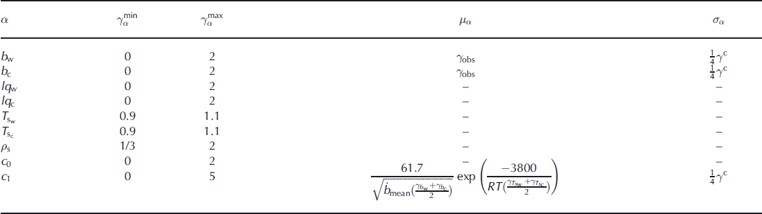
where lq is the liquid water content at the surface and T s is the surface temperature, both given for each time-step in the firn model by the RCM. Given the possibility of seasonal differences in the external forcing parameters, the tuning factors are split into two components. The subscript ‘w’ refers to warm months (May–October) and ‘c’ refers to cold months (November–April). Several of the tuning parameters are co-dependent, therefore a number of model experiments are performed to find the optimal set of tuning parameters. In addition, the optimal set of parameters might be site-dependent.
We use a Monte Carlo method to investigate our model parameter space statistically. The Metropolis algorithm (Reference Mosegaard and TarantolaMosegaard and Tarantola, 1995) guides the random walk in the nine-dimensional model parameter space defined by γ. A model solution, d j , at a node point, j, in the random walk is given by
where g is the forward model (Eqns (1), (3), (5) and (12)). The a posteriori probability, ξj , at the node point can be computed from the likelihood, Lj , and the a priori information, μj :
where k is a normalization factor. The likelihood of a model solution based on the observations, d obs, is given by

where the observations are assumed to have a Gaussian distribution of the associated error distribution given by the covariance matrix, C obs. The a priori probability is based on our physical understanding of the model space, γ, and is the only way of limiting the random walk in the parameter space. Depending on the type of a priori information available for a specific parameter, a flat or Gaussian probability distribution is applied as a priori information. The resulting μj is given by the product of the individual a priori probability distributions. At a given node in the random walk, the model solution is accepted with the probability

where ξi is the a posteriori probability of the previously accepted node in the random walk. The possible acceptance of models with a probability <1 makes the random walk capable of jumping out of a local minimum in the parameter space. The work flow of the Monte Carlo inversion is illustrated in Figure 2.

Fig. 2. Flow chart of the Monte Carlo inversion and the elements of the firn-compaction model.
When a sufficient number of accepted solutions have been found by the random walk, the solution to the inverse problem is given by the distribution of the accepted models. The solution distributions often show multiple peaks, and the Expectation-Maximization (EM) algorithm (Reference McLachlan and PeelMcLachlan and Peel, 2000) is used to estimate the most likely solution. The EM algorithm finds the maximum-likelihood estimate for parameters in a Gaussian mixture model of the nine-dimensional model parameter space. In the following, a mixture of three Gaussian distributions is used.
Firn model initialization
Initialization of the dynamical firn model is needed, as the firn model describes the addition of firn layers on top of a pre-existing firn surface. As initial conditions, we use the steady-state firn-compaction model of Reference Herron and LangwayHerron and Langway (1980) with the inclusion of ice lenses (Reference ReehReeh, 2008) and the isothermal compaction-rate constants of Reference Arthern, Vaughan, Rankin, Mulvaney and ThomasArthern and others (2010). The model assumes the 1989–2009 average climate from the HIRHAM5 RCM, and provides a mean density profile for the site for equally spaced layers in the firn. It is thereby a computationally efficient representation. With compaction rates given by the model, the steady-state density profile is interpolated onto the time domain used by the dynamical firn-compaction model.
The dynamical model starts in January 1989 (the start of the HIRHAM5 RCM record), by adding monthly layers to the surface. The combined initial steady-state firn model and dynamical firn model will affect the firn-temperature profile towards the annual mean for the first few months after January 1989, but the effect gradually deceases.
Firn-Core Experiments
At the two firn-core sites a number of inversion experiments were performed to evaluate the biases associated with (1) limited a priori knowledge, (2) the type of observation used in the likelihood calculation, (3) the degrees of freedom in the inversion and (4) model parameter choices. The experiments aim to estimate the uncertainties in the inversion of firn-compaction parameters using observed layers from firn radar data. The experiments for the two firn-core sites are summarized in Table 1. The a priori information applied is listed in Table 2, which is based on physical considerations of the model system and initial tests of the Monte Carlo inversion.
Firn compaction in the dry-snow zone is less complicated than when meltwater is involved, which makes the NEEM site ideal for evaluating the model and the inversion biases, without the additional uncertainties of water retention. The nine-dimensional model space may be reduced in dimension if some of the γ-parameters are strongly correlated, or negligible. In addition to the internal model processes, the external forcing may also bias the outcome of the inversion. The HIRHAM5 RCM forcing is limited to the period 1989– 2009, and therefore the firn layers can only be dynamically modeled for this period. Eight inversion experiments were performed for the NEEM site (Table 1) to test the response of altering the initial set-up described above. The first six experiments (F1–F6) use the full observational dataset from the NEEM firn core to constrain the inversion, whereas the last two (L1 and L2) investigate the bias when limiting the observational dataset to the period 1989–2009. The inversion experiments are: (F1) Inverting for all parameters in the model space. Applying the mean observed accumulation rate from the ice cores as Gaussian a priori information and both the observed chronology and the density profile of the core in the likelihood calculation. (F2) As F1, but assuming γT sw = γT sc = 1. (F3) As in F1, but assuming γlq w = γlq c = 1. (F4) Removing the seasonality in the tuning of the external forcing: γb w = γb c, γlq w = γlq c, and γT sw = γT sc . (F5) Combining all the assumptions of F2–F4. (F6) Not using the Gaussian a priori information of the mean accumulation. (L1) Using only the density profile to the depth of January 1989 in the likelihood calculation. (L2) Using only the chronology from the surface to January 1989 in the likelihood calculation.
The Flade Isblink site experiences repeated melt events during the summer months, which makes the modeling more complicated. The observations from the Flade Isblink firn core were used to test the choice of ρ ip in the retention scheme. Since ρ ip controls the depth at which the water can percolate, it is the main constraint on water percolation. Based on the change in firn properties around 830 kg m−3, three experiments were performed: (I1) ρ ip = 700 kg m−3; (I2) ρ ip = 830 kg m−3; and (I3) ρ ip = 917 kg m−3. The three experiments were performed using a homogeneous probability-density distribution (Reference TarantolaTarantola, 2005) for the a priori information for γc 1, since the observed density at the site will constrain γc 1.
Results
NEEM site: dry case
Experiment F1 is denoted the control experiment, since it applies all available information for the inversion, whereas F2–F6 evaluate the bias when limiting the model parameter space or the a priori information. Reducing the model parameter space by one parameter at a time (F2 and F3) results in a higher root-mean-square error (rmse) than in the control experiment, as shown in Table 3. This indicates that all the tuning parameters are necessary for the model to have the right degrees of freedom. Experiment F4 neglects the seasonality of the external forcing tuning parameters, which again results in an increased misfit to the observations. Reducing the number of model parameters to an absolute minimum (experiment F5) reduces the misfit compared with F1. However, the limited surface melt at the NEEM site results in a less constrained value of γlq , which may increase the misfit. Therefore, when assuming γlq = 1, as in experiment F5, the unconstrained γlq does not affect the final result. Assuming γlq = 1 may be a good approximation at NEEM, but may not be valid for the entire GrIS firn-covered area. Finally, the F6 rmse is lower than found for the F1 experiment, which suggests that the initial inversion set-up (F1) is over-constrained, and that the information used in F6 is sufficient to constrain the inversion. The γρ s, γc 0 and γc 1 model parameters for F6 are all well determined by the inversion and exhibit a low coefficient of variation (σ/γ ∼ 0.08), while the external forcing tuning parameters result in a higher coefficient of variation (σ/γ ∼ 0.22), which may be considered the accuracy of the inverted parameters. Further, the RCM output field provides a mean annual accumulation at the site of 18.4 cm, which is significantly lower than the annual accumulation of 22.7 cm ice equivalent from ice-core measurements. After tuning, the mean annual accumulation is 21.9, 22.1, 25.7 and 23.0cm for F1, F6, L1 and L2, respectively. For all the experiments except L1, this is within the error of the observation. In addition to the RCM output accumulation rate field being too dry, the results of the inversion indicate that the deviation of the RCM output accumulation rate is stronger in cold months than in warmer months at the NEEM site.
Table 3. The result of the inversion experiments performed at the three sites. The results for the ASIRAS radar inversion are only expressed as the mean of Figure 6b. For the EGIG-line ASIRAS result, the root-mean-square error (rmse) is derived as the mean of the 20 individual inversions performed in the test area, in units of air-equivalent radar travel (m)

The two additional inversion experiments, L1 and L2, are performed to investigate the bias of limiting the observations used in the inversion. Additional a priori information is needed to constrain the tuning of the second-stage firn compaction, γc 1, if the observational dataset is limited to densities less than ρ c. The results of γc 1 in F1–F6 all agree with the predicted value based on Eqn (4). Hence, a Gaussian a priori for γc 1 is added to constrain the second-stage firn compaction based on Eqn (4) (Table 2).
Figure 3 shows the results for F6, L1 and L2. A common feature of the modeled densities is the deviation from the observations at 1 m below the January 1989 layer (marked by a horizontal line in the right panel). This is an artifact of the transition from the steady-state initialization to the dynamic firn-compaction model, which can be expected due to the model set-up. Both F6 and L1 result in similar densities in the top firn, while L2 tends to overestimate the surface density at the site and underestimate the compaction rate (Fig. 3; Table 3). This is also reflected in the increased coefficients of variance, σ/γ, of γρs and γc 0 for L2, which are almost double that of F6.

Fig. 3. The NEEM inversion results for experiments F6, L1 and L2, compared with the observations at the site (in red). The panels on the left show the symmetrical correlation matrices for each of the three experiments. The difference between the experiments is illustrated by the correlation matrices. The panel on the right shows both modeled densities and ages for the three experiments. The transition from dynamic to initialized firn modeling at the beginning of January 1989 is marked with the horizontal line, and ρ c is marked with the vertical line.
The difference between the F6, L1 and L2 results for the NEEM site firn core can also be seen in the correlation matrices in Figure 3. The fully constrained F6 experiment shows a strong (< −0.8) negative correlation between the modeled parameter tuning for warm and cold months in accumulation, and for the surface density and c 0, as illustrated in the upper left panel of Figure 3. This correlation indicates a trade-off between γb w and γb c and also γp s and γc 0 in the accepted solution of the random walk. The correlations between the two accumulation parameters are constrained by the chronology, whereas the correlation between γp s and γc 0 is constrained by the density information. This also explains why the L1 experiment only finds an anticorrelation between γp s and γc 0 and L2 only finds an anticorrelation between γb w and γb c, as seen in the left column of Figure 3. As seen in Table 3, the L1 inversion obtains an optimal fit with observed densities by increasing the annual accumulation by ∼10% compared with F6, which results in a rmse of 1 year in the modeled age. The L2 experiment finds the optimal parameter set with an increased surface density, which introduces a higher rmse for density.
The rmse normalized with respect to the F6 rmse, gives L2 the lowest combined error followed by F6 and F5, while L1 has the highest normalized error, mainly attributed to the misfit of 1 year in the model age, as seen in Figure 3. The normalized rmse for L2 is smaller than for L1, which indicates a better constraint of the combined product of firn compaction and external forcing by only applying information about the chronology in the inversion, as in experiment L2.
Flade Isblink: wet case
The model results, shown in Figure 4, indicate the model is capable of reproducing the mean densities and the chronology at the Flade Isblink site in all experiments, but neither high- nor low-density peaks in the density profile are captured by the model. Both the minimum and maximum peaks in density can be explained as resulting from neglecting horizontal movement of percolating meltwater in the model and the time discretization of the model. Neglecting the horizontal movement of water flow affects the modeling result in two steps. First, horizontal water flow would be directed along ice lenses, increasing the density around these. Second, due to the missing addition of mass with depth, the inversion tries to find the optimal model parameters in order to fit the density profile by increasing the surface density (γρ s = 1.47 for I3). Both steps result in a limited precision of the error estimate based on the chronology measure. In addition, the rather coarse time discretization of the model will limit the formation of high-density layers in the firn profile (as short-lived percolation events (e.g. rain or strong melt events) are not included in the model) which might form ice layers in the top firn. These layers may be additionally enhanced at later percolation events and thereby be an important feature in the formation of high-density layers.
The I3 experiment (ρ ip = ρ i) has the lowest density misfit for the inversions and is therefore favored as the best representation of the Flade Isblink firn column. This solution also shows two promising features: (1) A decrease of the modeled densities dated to the 1990s, which is also seen in the observations. This is a prominent feature that might be enhanced if horizontal water flow were allowed. (2) The correlation matrix of I3 shows an anticorrelation for the parameter pairs (γb w, γb c) and (γlq w, γlq c) and a less-noisy correlation matrix than I2 (Fig. 4). When the experiments are compared, ice lenses are the only real obstacle for the water percolating in the firn. Therefore, the initialization of the firn does not bias the dynamically driven layer above. As observed in Figure 4, the uppermost density is increased from experiment I1 to I3; this can be attributed to the run-off criteria in the model description, which removes the water when downward motion is ceased. The latent heat release at sites like Flade Isblink is an important heat source in the modeled temperature profile. A comparison with borehole temperatures at the site showed that the modeled temperature profile is biased towards lower temperatures, due to difficulties in estimating the cold content of the initialized temperature profile. This suggests that the temperature inversion is less constrained by the in situ parameters, which is expressed by the high standard deviation of the temperature tuning, compared with its a priori information

Fig. 4. The results of the Flade Isblink inversion experiments and observations at the site. The correlation matrices for each experiment are shown in the left panels. The right panel shows the modeled densities and ages.
The result for the RCM tuning indicates an overestimation of the precipitation by the RCM output files (Table 3). This suggests that the RCM tends to deliver too much precipitation at the margin of the GrIS (as seen at the Flade Isblink site), and be too dry in the interior, as observed with the NEEM site inversions. The high γρ s combined with high temperatures at Flade Isblink results in high-density layers being deposited at the surface by the model. Since the mean density profile is captured by the model (Fig. 4) the high-density surface layers cannot explain the γc 1 < 1 found in all of the experiments.
EGIG line: spatial case
Figure 5 shows the 2008 ASIRAS radar data along with the modeled depth of annual layers using the tuning parameters determined in the NEEM F6 experiment. The strong reflections in the radar data have previously been associated with deep hoar formation in the fall (Reference De la PeñaDe la Peña and others, 2010). However, such microphysical processes are not modeled here, and we assume that the annual stratification is represented by the modeled October layer. The modeled thickness of the annual layers are in good agreement with the first few observed layers, but the agreement tends to deviate with depth. In particular, the thinner layers on the eastern side of the GrIS ice divide (located at ∼35° W) are not captured by the modeled layers when using the parameters inferred from the NEEM F6 experiment. The deviations between the observed firn layers and the layers modeled using the parameters found for the NEEM F6 experiment emphasize the need for a separate investigation of the tuning parameters at the EGIG line. In the shaded box in Figure 5, the difference between the observed and modeled layers changes sign at ∼38° W. Several causes can be given for this (e.g. the HIRHAM5 RCM forcing could be biased, the firn-compaction model could be biased in the physical description or the spatial/temporal patterns of the tuning parameters could vary over the GrIS). To investigate this, an inversion for the tuning parameters is performed at each of the 20 HIRHAM5 RCM gridpoints in the selected area on the EGIG line. The inversion follows the method developed for the NEEM L2 experiment with ρ ip = ρ i, since the radar data only provide countable layers and no information on densities. In the selected area of the EGIG line, the slope of the isochrones is small and the seasonal melt is almost absent, reducing the uncertainty of the inversion. Figure 6a shows the result of the inversion for the most likely solution, along with the traced ASIRAS layers. All three Gaussian distributions found by the EM algorithm are shown as contours in Figure 6b, where the Gaussian distributions have been normalized in accordance with their probabilities found by the EM algorithm. The solution illustrated in Figure 6a is assigned a >50% probability by the EM algorithm for the majority of the inversion points. However, the two remaining solutions (not shown in Fig. 6a) at each point cannot be discarded as bad representations of the firn, with the biases found by the NEEM L2 experiment in mind. Quantitative comparison with Reference Morris and WinghamMorris and Wingham (2011, their fig. 2) shows that the three solutions of the EM algorithm capture the observed densities, with a slightly higher density in the high-density layers. This suggests that studies of surface density should be conducted at locations with a good instrumental record of forcing parameters, in order to be sure the inversion is well constrained and allowing the surface density to be the primary unknown in the inversion. However, this is beyond the scope of the present study.

Fig. 5. The 2008 ASIRAS radar image with modeled October layers estimated using the model parameters determined in the NEEM F6 experiment. The observations and modeled layers are in good agreement for the first few layers and then gradually deviate with depth. The thinner layers on the eastern side of the ice divide, especially, are not well represented by the model. The ice divide can be identified in the image by the change in slope of the layers at ∼35° W. The shaded area (∼37−39° W) was selected for further inversion studies (Fig. 6) using the ASIRAS radar data as observational input for the inversion method developed for NEEM site L2. The depth scale is in air-equivalent radar travel distance.

Fig. 6. The result of firn-compaction inversion using the ASIRAS radar data for the section of the EGIG line shaded in Figure 5. The mean rmse between the modeled and observed layers is only 9 cm, which is within the error of the layer tracing. (a) In blue are the traced layers from the 2008 radar image, and stars indicate the locations of the modeled annual layers at each of the 20 HIRHAM5 gridpoints. The depth scale is in air-equivalent radar travel distance. (b) Contour plot of the normalized probability distribution based on the EM algorithm for each of the 20 gridpoints. The grid numbers are shown in (a).
Table 3 lists the mean of the preferred tuning parameters of the individual inversions performed on the EGIG line. The rmse of the observed layer depth is 9 cm, which is equivalent to the standard deviation of the traced layers in the area. As seen in Figure 6a, the interannual variability in layer thickness along the 67.5 km of the EGIG line is captured by the model. This interannual variability in the layer thickness is not tuned by the inversion scheme, since the same seasonal tuning is used for all layers at a HIRHAM5 gridpoint. Hence, this suggests that the HIRHAM5 RCM output fields provide accurate temporal variation in the forcing field to the firn model. The average of the inverted parameters for the HIRHAM5 RCM at the EGIG line is similar to the NEEM results, both in absolute magnitude and in uncertainty, again indicating that the RCM output fields underestimate the inland precipitation on the GrIS.
The results of tuning the firn parameters, γρ s, γc 0 and γc 2, are not as straightforward to interpret. The limited uncertainty found for γc 1 on the EGIG line may be attributed to the a priori information applied, and, as illustrated by the spread of EM solutions for γc 0 in Figure 6b, the tuning parameters are not well determined and show high spatial variability. The average of the 20 individual inversion results gives γc 0 = 1.4 and γρ s = 0.73. The value of γc 0 is therefore significantly higher than found at the NEEM site. The NEEM L2 experiment tended to overestimate γv s when only the chronology was applied as prior information (Table 3). This is not seen in the mean solution of the EGIG inversions, where the surface densities have to be increased to be comparable with the NEEM result. If the anticorrelation of the two parameters as found at NEEM is interpreted as a linear relationship, a 0.1 increase in γρ s would only result in a reduction of γc 0 to 1.27. Therefore, the lack of correlation between the two parameters cannot explain the significantly higher firn-compaction rates found on the EGIG line than at NEEM. This indicates a site dependency of the compaction-rate factors, which cannot be reproduced by the firn parameterization used here.
Discussion
Our experiments at the two firn-core sites show that the initial model set-up is capable of describing the firn compaction when both the observed chronology and the density are used as prior information. Here the rmse (Table 3) indicate the inversion is well constrained. However, if more information is used the inversion may become overdetermined, as seen in the difference between NEEM experiments F1 and F6, while experiment F4 showed that the seasonality of the tuning parameters adds the appropriate degrees of freedom to the system to accurately model the observations.
The normalized rmse with respect to experiment F6 is smaller for experiment L2 than for experiment L1, indicating a better representation of the modeled firn compaction by the NEEM L2 experiment. This difference in normalized rmse between NEEM experiments L1 and L2 indicates that the chronology provides good prior information to constrain an inversion of both the firn-compaction model parameters and RCM output field tuning. The less-constrained tuning parameters of the external forcing fields in the L1 experiment imply that any updated/developed firn-compaction model is limited by the accuracy of its external forcing if only the observed density is used in its validation. The NEEM L2 experiment tends to overestimate the densities in the upper firn, as shown in Figure 3. This overestimation in first-stage densities is a result of the limited correlation between γρ s and γc 0, as shown in the lower panel of Figure 3. Therefore, following the method outlined in the NEEM L2 experiment may lead to a misinterpretation of the tuning parameters for ρ s and c 0.
Percolation in polar firn has been observed to be highly heterogeneous (e.g. Reference Humphrey, Harper and PfefferHumphrey and others, 2012) and not only confined to vertical water flow. Also, the timing of the percolation events may be crucial to the formation of ice lenses. The presented water retention scheme only allows for water to percolate downward by gravity and simple volume/ energy considerations, evaluated at a monthly time-steps. This model description may be seen as a first-order approximation for water percolation and refreezing, which is only valid for areas with little melt. However, the Flade Isblink results show that the model is capable of representing the mean densities at a high-melt site. Confined to 1-D flow, the controlling factor for water retention is the density of the impenetrable layers, where ρ ip = ρ i gives the best fit to the observations. The model cannot redistribute mass horizontally, and therefore the modeled firn column indicated there was a missing mass input, which was also suggested by the increase in the rmse as water flow was limited. Further, in high-melt areas the model set-up will be highly biased by the time discretization applied here, and the precision of the present model set-up will be diminished. For example, a short-duration event (e.g. rain or strong melt and subsequent refreezing of percolated meltwater) would not be resolved by the monthly resolution of the model. To include such events in more detail, a full coupling to a RCM is needed, which is beyond the scope of this work, but would be an important next step for future modeling efforts. However, the first-order approximation of gravity-driven retention may be applied in areas where the slope of the ice sheet is sufficiently small to confine the water routing to the vertical direction. This is the case for the central part of the ASIRAS radar profile, where the radio-echo data show little evidence of meltwater percolation.
The results of the NEEM and Flade Isblink experiments suggest that radar data, providing chronology information, can be used directly for inversion studies of firn-compaction rates. The firn-compaction tuning parameters may be biased by limited correlation between ρ s and c 0, as found in experiment L2. Based on the favored solution by the EM algorithm, the difference in the tuning factors for the NEEM site and the EGIG line cannot be directly linked to the difference in the accumulation and surface temperatures at the two sites. This suggests that other factors that are not included in our model also affect the densification rate. A previous study by Reference Hörhold, Kipfstuhl, Wilhelms, Freitag and FrenzelHörhold and others (2011, Reference Hörhold, Laepple, Freitag, Bigler, Fischer and Kipfstuhl2012) suggests that observed firn-compaction rates at their study site were related to the impurity content of the firn, a factor that would be different at the NEEM and EGIG sites. The EGIG study also supports less-likely solutions, with similar values for γc 0 to those found at NEEM, as seen in Figure 6b. Therefore, the inversion experiment should be extended to include more of the GrIS, before any conclusions about spatial variability of the firn-compaction factor can be drawn. The model tuning of the second stage of firn compaction showed a slower firn-compaction rate than the parameterization by Reference Arthern, Vaughan, Rankin, Mulvaney and ThomasArthern and others (2010), even at the Flade Isblink site, where water is assumed to saturate the firn column. This suggests that the Reference Herron and LangwayHerron and Langway (1980) compaction-rate constants can be applied for the firn compaction of the second stage on the GrIS, when annual temperature variations are dampened and the firn is approaching isothermal conditions. This result is in agreement with the study of Reference Ligtenberg, Helsen and Van den BroekeLigtenberg and others (2011), who also showed an accumulation dependency of the second-stage densification.
Having a set of radar data separated by 2 years should be sufficient to measure direct compaction over the entire EGIG line without introducing a model. However, the signal-to-noise ratio is too large to obtain any useful information when subtracting the two images from each other. Therefore, the signal-to-noise ratio of the radar needs to be improved before direct observation of firn compaction can be obtained from the radar data alone, without additional firn modeling. As shown, the rmse at the EGIG line is already equivalent to the standard deviation of the traced layers in the radar data from 2008.
Conclusions
The method developed and validated here can be used to assess firn-compaction rates from firn radar data. This new approach provides important information about both the external forcing and the internal parameters in the firn-compaction model. The inversion experiments indicate spatial variation in the firn-compaction rates, which cannot be attributed to biases in the external forcing only. Based on the firn-core experiments, the inversion of firn-compaction parameters is well constrained when both the firn chronology and density are used as prior information. Biases in the external forcing or the firn-compaction parameters are not as well constrained if only one type of information is applied. However, the experiments indicate that using the chronology alone as a constraint results in minor biases of the firn-compaction model-tuning parameters. The tuning parameters found for the first-stage compaction rates give no conclusive evidence for a deviation from the Reference Arthern, Vaughan, Rankin, Mulvaney and ThomasArthern and others (2010) parameterization, but the results from the ASIRAS measurements indicate that the parameterization is site-dependent and cannot be defined by temperature and accumulation alone. Both firn-core sites support a reduction of the second-stage firn-compaction rates, compared to those reported by Reference Arthern, Vaughan, Rankin, Mulvaney and ThomasArthern and others (2010), as also found by Reference Ligtenberg, Helsen and Van den BroekeLigtenberg and others (2011). Since the available radar data are too shallow to resolve this properly, more ice-core data or deeper-penetrating radar data are needed to confirm this for the GrIS.
Using radar data to assess firn-compaction rates over large spatial distances can provide information on the spatial variability of the firn behavior in the future, which cannot be investigated by firn cores alone. This work is timely because new high-resolution radar data are becoming available, for example with the development of new instruments by the Center for Remote Sensing of Ice Sheets (CReSIS), at the University of Kansas, collecting data as part of the NASA IceBridge mission.
Acknowledgements
We acknowledge the Danish National Research Foundation for funding. We thank Henrik B. Clausen, Susanne L. Buchardt, Anders Svensson and the Flade Isblink and NEEM teams for providing the firn-core data, and Michelle Koutnik for valuable suggestions for improving the manuscript. We acknowledge the huge efforts of the CryoSat validation and retrieval team (CVRT) in collecting ASIRAS data during the CryoSat Validation Experiment (CryoVEx) campaigns. Finally, we acknowledge two anonymous reviewers for insight into the subject of firn compaction, which also helped to improve the manuscript.


