

Introduction
In the glaciological community there is a need for reliable mass-balance measurements of glaciers and ice sheets ranging from daily to yearly timescales. These in situ data are needed to validate remotely sensed estimates and melt model calculations around the world (Reference Dahl-JensenDahl-Jensen and others, 2009). A common method for determining ablation is to use stakes, which are drilled into an ice surface and record the ablation through their free length at every visit. This provides fairly accurate information on surface melt, but only gives totals over the period since the previous stake visit. For remote areas such as Greenland, where stakes cannot be read more than once or twice per year even in the most accessible locations, these infrequent visits do not allow interpretation in terms of melt variability or length of the melt season.
Sonic rangers mounted on stakes are also commonly used to measure surface ablation or accumulation at any time interval. A problem with these instruments is that the quality of their readings reduces in time as they degrade due to continuous freeze-thaw cycles in a generally moist climate (Campbell Scientific, 2011). A greater problem is that sonic ranger stake assemblies need to be revisited and re-drilled before they melt out or collapse due to strong winds. Additionally, the range of these instruments is limited to ~10m (Campbell Scientific, 2011). In Greenland, ice ablation values of up to 9m in a single year have been reported (Reference Van AsVan As and others, 2011), and values exceeding 5 m are common at low elevations on the ice sheet (Reference Fausto, Van As, Bennike, Garde and WattFausto and others, 2012), creating the need for an alternative method. Realizing the shortcomings of such measurements, Reference HulthHulth (2010) presented a draw-wire method to measure glacier melt continuously without the use of stake assemblies, which shows promise of being able to provide reliable and continuous in situ ice ablation measurements.
In this paper, we discuss and improve a fourth method for measuring ice ablation, which was first used by Reference BØggild, Olesen, Ahlstrøm and JørgensenBØggild and others (2004). In 2001, they introduced an ablation assembly consisting of a hose filled with antifreeze liquid with a pressure transducer located at the end/bottom. This set-up has been in development at the Geological Survey of Denmark and Greenland (GEUS) in recent years, though the basic design and measurement principle has remained the same (Fig. 1). The hose is drilled into the ice using a mechanical or steam drill. The sensor cable runs inside the hose until it exits the closed system above the ice surface, and is connected to the data logger of an automatic weather station (AWS). A liquid-filled bladder at the top end of the hose provides a stable upper bound for the vertical liquid column over the pressure transducer, and accommodates volume changes in the liquid or the hose itself so that pressure fluctuations in the assembly are minimized. The pressure signal registered by the transducer in the ice is that of the vertical column of liquid over the sensor, which can be translated to depth knowing the density of the liquid. As the free-standing AWS moves down with the ablating surface and the hose melts out of the ice, an increasingly large part of the hose will lie flat on the ice surface, and the hydrostatic pressure from the vertical column of liquid in the hose will decrease. This reduction in pressure provides us with the ablation rate. The period over which this set-up can be used depends on the local ablation rate.

Fig. 1. Graphic representation of the pressure transducer assembly.
Pressure transducer assemblies (PTAs) have been installed at all the AWSs in the Programme for Monitoring of the Greenland Ice Sheet (PROMICE) (Ahlstrom and others, 2008; Reference Van AsVan As and others, 2011; Reference Fausto, Van As, Bennike, Garde and WattFausto and others, 2012). The PROMICE network in Greenland, initiated in 2007, currently consists of eight transects of two to three AWSs at different elevations (Table 1; Fig. 2). Each station measures all relevant meteorological parameters and ice and snow ablation; the instruments are shown in Figure 3. The number of data collected since then allows the accuracy of the current PTA design to be investigated, as was done in a pilot study by Reference BØggild, Olesen, Ahlstrøm and JørgensenBoggild and others (2004). In this study, we describe the modifications the PTA design has undergone since 2001. We describe the routine to transform raw measurements into ablation values, including a physically based method to remove air-pressure variability from the signal. Finally, we compare pressure transducer time series to those recorded by manual hose measurements and sonic ranger in order to quantify the inaccuracies of this instrument.
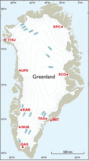
Fig. 2. Map of Greenland showing the locations of PROMICE AWS with PTA. Each dot represents a minimum of two stations of which the lower one is labeled ‘_L’ and the upper one ‘_U’.

Fig. 3. PROMICE AWS set-up from UPE_L photographed on 17 August 2009: 1. radiometer; 2. inclinometer; 3. satellite antenna; 4. anemometer; 5. sonic rangers; 6. thermometer and hygrometer; 7. PTA; 8. solar panel; 9. data logger, barometer and GPS; 10. battery box with 4˟ 28 Ah batteries; 11. eight-level thermistor string.
Table 1. PROMICE automatic weather stations with a PTA (status 2011)

Method
Deployment history and development
The first deployment of a PTA to measure ice ablation was in 2001 on the Qassimiut lobe, South Greenland, followed by more assemblies in 2002 (Reference Podlech, Mayer and BøggildPodlech and others, 2004). This region is characterized by high surface melt values compared to most other locations on the Greenland ice sheet, with ablation totals exceeding 5 m a-1, making it impossible to use sonic ranger stake assemblies without having to visit them twice per year. In the following years, pressure transducers were also installed elsewhere on the Greenland ice sheet: three in the Nuuk region in 2003, two in the Tasiilaq region in 2004 and one in the Melville Bay region, northwest Greenland, in 2004 (Reference Van AsVan As, 2011). Since then, GEUS has installed PTAs at all AWSs in the ablation zone, most of which are included in the PROMICE station network. Reference BØggild, Olesen, Ahlstrøm and JørgensenBØggild and others (2004) showed that the first results were promising and that the design had great potential for measuring ablation in remote and seldom- visited places. However, the two sites discussed by Reference BØggild, Olesen, Ahlstrøm and JørgensenBØggild and others (2004) and Reference Van AsVan As (2011) indicate that the original design of the system required improvement.
The current design of the PTA is as follows (Fig. 1). An NT1400 absolute pressure transducer manufactured by Ørum & Jensen Electronik AS in Denmark is enclosed in an armoured rubber 19.05 mm (0.75 in) hose with a total length of ~25 m. The pressure transducer is secured to a 20 cm long and slightly larger than 19.05 mm iron rod which is inserted in the bottom part of the hose with silicone sealant and fastened with hose clamps. The rod functions both as a watertight seal and weight. At the upper end of the hose a T-junction is inserted to allow the logger cable going out of the closed PTA system to connect the pressure transducer to the logger. The other branch of the T-junction is connected to a 2 L expansion bladder. The bladder is roughly half-full to allow volume changes in the antifreeze (e.g. by solar heating) without leading to a pressure build-up in the assembly. A bladder enclosure is mounted on the mast of an AWS in order to have a fixed reference point for the height measurement recorded by the PTA. The antifreeze is a 50/50 water and ethylene glycol mixture, which has a freezing point of –34°C, making it applicable to most places in Greenland. Furthermore, we made hose markings of 2 m distance to the pressure transducer for an easy manual ablation measurement during a station visit.
In recent years we have modified the PTA to optimize performance and in-field practicality. The original PTA design made use of relative pressure transducers, which require an open connection to the atmosphere, to be able to compensate for barometric pressure variability. The relative pressure transducer thus had a 1 mm air-filled tube inside the connecting cable running from the sensor to the surface inside the borehole. To avoid closure of this delicate tube under pressure of the ice and/or snow on the cable going to the logger box, and to simplify the assembly altogether, we started using the absolute pressure transducer, which does not require an open-air connection. We changed the liquid in the PTA from alcohol to a 50/50 mixture of water and ethylene glycol, which is less volatile, easier and cheaper to import and has a density closer to that of ice. The 6.35 mm (0.25 in) fiber-reinforced PVC hose was exchanged for a 19.05 mm (0.75 in) hose, and the transmitter cable was inserted to avoid potential damage to the cable. In the original design, a custom-made T-junction was welded onto the pressure transducer and attached to the 6.35 mm (0.25 in) alcohol-filled PVC hose connected to an expansion bladder lying on the ice surface. This proved to be a poor solution because the flexible PVC hose attached to the T-junction could not be efficiently closed off to keep the volatile alcohol contained. In the new design, we moved the T-junction up to the AWS where it is secured with the expansion bladder in an enclosure mounted on the mast (Fig. 1). Moreover, the hose of the PTA was shortened from ~40m to 25 m for reasons of practicality. This reduces weight and volume in shipping and transportation onto the ice sheet by helicopter. Installing the pressure transducer at 20 m depth is sufficient for a 3–6 year deployment in the high-melt regions of the Greenland ice sheet. After this period we replace the PTA and take back the old one to check for drift in the output signal and to recalibrate. A longer deployment in the field does not allow for regular calibrations. Furthermore, in the original design of the PTA, the expansion bladder was lying free on the glacier surface, sliding to the lowest point in the immediate surroundings. In the current design, the bladder is placed in an enclosure on the AWS mast. Keeping the bladder fixed and in an enclosure protects it from the elements and provides a potentially constant reference level for the pressure transducer, except when the AWS lowers with the ablating surface. The enclosure is typically placed ~1.5 m above the ice surface. The potential tilt of an AWS could result in a vertical change in the position of the bladder, thus affecting the height of the vertical liquid column over the pressure transducer, but this set-up gives more stable pressure transducer signals than before the usage of the bladder enclosure as it cannot slide or be blown around the ice surface.
Data processing
The PROMICE AWSs measure and store data every 10min with the exception of the wind speed observations that give the mean wind speed since the last measurement cycle, and the GPS measurements, which follow the transmission schedule. During summer (days of year 100–300) the values are transmitted hourly. During winter (days of year 301–99) the measured quantities are transmitted once a day at midnight to limit power consumption when solar power is not available. The transmissions consist of average values (daily or hourly) of the more transient quantities (e.g. temperature or radiation). Instantaneous values of less transient quantities (e.g. surface height by PTA and sonic ranger and station tilt) are appended once every 6 hours in summer and once a day in winter for all daily transmissions.
In processing the pressure transducer data, the voltage output recorded by the data logger, V is calculated into measured height of the vertical liquid column, HM , using a multi-point calibration:
The calibration coefficients a and b are provided by the pressure transducer manufacturer for application in water, and also reproduced at GEUS after assembling the PTA. The former coefficients require a multiplication factor to compensate for the density change introduced by the application with antifreeze. The latter method is also used for recalibration after retrieval from the field.
Because we use absolute pressure transducers, the PTA measurements also include barometric pressure, PA. The measured pressure, PM, is thus calculated as
where PL is the pressure exerted by the vertical liquid column and PC is the (known) pressure at which the sensor was calibrated (so that PM is near zero when the pressure transducer is not submerged in liquid). Using the hydrostatic equation
in which pL is the density of the antifreeze mixture (at 0°C pL ≈ 1090 kg m-3) and g is the gravitational acceleration (9.81 ms-2), and assuming an insignificant influence from the density of the atmosphere, pA, so that

we then find

Ice ablation is then equal to changes in H L.
Results
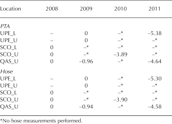
Data from five PROMICE AWSs located in three distinct regions (SCO, UPE and QAS; Fig. 2) are used in this assessment of the PTA. At the SCO and UPE sites, we use both the upper and lower AWS in order to include possible altitudinal effects on the assessment of the PTA. The five AWSs are all equipped with a PTA and two Campbell Scientific SR50A sonic rangers that allow us to monitor surface height change due to accumulation and ablation (Fig. 3). Furthermore, during maintenance visits, the length of the melted-out part of the PTA hose was measured at three of the stations (Table 2), which should form a manual and independent observation that can be compared to the PTA measurements.
Table 2. PTA vs manual on-site hose measurement (m ice eq.) relative to the ice surface
Ablation records for pressure transducers in Greenland
Figure 4 shows 1 year of PTA measurements at the SCO_L station, and shows the need for removal of air-pressure variation from the pressure transducer signal. The recorded air pressure correlates with the pressure transducer signal and can explain 99% (r2 value), on average, of the variability during the accumulation season (accumulation is not recorded by the PTA). Removing the influence of the air pressure lowers the standard deviation of the pressure transducer, on average, from 9 cm to 1 cm for the selected test sites (Tables 2 and 3). Naturally, the influence of the air pressure for the ablation period is also removed, which is only slightly visible in Figure 4, because the variability in the pressure transducer signal is dominated by ice ablation.

Fig. 4. Calibrated ice height measurements by pressure transducer at AWS SCO_L before (black) and after barometric pressure compensation (blue). Barometric pressure at the stations is given in red.
Table 3. Root-mean-square difference (RMSD; cm ice eq.) and correlation coefficient (r 2; %) between PTA and sonic ranger

Figure 5 shows the full ablation record as obtained by the pressure transducer for SCO_L from installation in 2008 until 2011. Negative values indicate the amount of glacier ice that has ablated since installation. In this period, the annual net ablation values ranged from 2.5 to 4 m of ice. The figure shows both the raw and processed data for the full period, again illustrating the importance of applying the density correction and barometric pressure compensation to the data to obtain a reliable ice ablation record. The cumulative ablation over the period shown exceeds 10 m of ice, which was captured well, without the need to perform maintenance over the interval.

Fig. 5. Ice level measurements before and after calibration plus barometric pressure compensation (PTA-corrected) for the full measurement period of SCO_L.
Assessment of the accuracy/uncertainty in ablation studies
The PTA is well suited to monitoring ice ablation in remote regions at sub-daily timescales, with clear advantages over other, well-established methods. For example, at every maintenance visit we perform stake readings, which provide information on surface height change but produce a low-frequency record as readings can only be done when the stakes are visited. All PROMICE stations have two Campbell Scientific SR50A sonic rangers equipped that allow us to monitor surface height change due to accumulation and ablation. The accuracy of the SR50A sonic ranger given by the manufacturer is ±1 cm or ±0.4% of the measuring height after temperature correction. This was confirmed for a 67day virtually accumulation-free, wintertime period at SCO_U, during which standard deviations of 1.7 cm and 0.6cm were found (after spike removal), which are 0.7% and 0.6% of the distance measured by the two sonic rangers, respectively. Before spike removal the standard deviation of the sonic rangers was found to be 4 cm on the AWS sensor boom and 6 cm on the stake assembly. However, the precision of the readings from these sensors will reduce in time as they degrade due to continuous cycles of moisture freezing on and melting off them. As mentioned, a major problem with sonic rangers in surface mass-balance studies is that they need to be mounted on stake assemblies drilled into the ice. During a single melt season these stake assemblies can melt out several metres, often causing them to move or even collapse during strong wind events.
In comparison, the PTA is operational until it has melted out of the ice, which can take several years depending on drill depth and local ablation rate. This reduces the need for annual station visits, and thereby the considerable expense associated with logistics in Greenland. The pressure transducer sensor has an accuracy of 2.5 cm given by the manufacturer (Ørum & Jensen Elektronik A/S). The mean standard deviation of the UPE and SCO pressure transducer readings outside the ablation season is found to be 1 cm, indicating only a small random error, comparable to that of the sonic ranger.
The accuracy of the pressure transducers is expected to degrade over time as they drift due to the continuous pressure on the sensor. Sensitivity drift defines the amount by which an instrument’s sensitivity varies as ambient conditions change. Here the sensitivity drift is the difference in slope of the best linear fit between the initial calibration and a recalibration. The manufacturer does not state any specifications on drift of the instrument. However, we performed new calibrations on two sensors that were brought back after years of deployment on the Greenland ice sheet to quantify the amount of drift on the sensor. The difference between the slope of the initial calibration curve and that of the recalibration was, on average, 1.6% for a 4 year period, which suggests that the sensor drift is not a major source of error in the pressure transducer system.
Intercomparison of in situ ablation measurements
Figure 6 shows transmitted (instantaneous values every 6 hours) data from SCO_L for 2011 as an example of a comparison between the PTA and the sonic ranger mounted on the stake assembly. The onset of melt and the general trend of the two measurements follow each other closely and have a correlation coefficient of >0.99 and a root-mean- square difference (RMSD) of 3.6 cm. Figure 6 shows a 100 day melt period during which the sonic ranger recorded a total ice ablation of 3.12 m compared to 3.14 m from the PTA, yielding a difference of 2 cm, or 0.64%. Together with Table 3, Figure 6 shows the general agreement between the two different ice ablation measurements. The correlation coefficients and RMSDs in Table 3 give an estimate of the agreement between the PTA and the sonic ranger. The assessment of the PTA compared to the sonic ranger does not account for inaccuracies due to solar heating and other forcings at sub-daily timescales, plus random error for both methods. Table 2 compares the limited manual measurements of the hose of the PTA during maintenance visits with the corrected pressure transducer signal logged by the data logger. The three AWSs are located in different areas of Greenland in order to assess the robustness of the system in several climate settings. All the manual measurements are within 8cm of the PTA signal, which again confirms the accuracy. The differences are more likely to be caused by the inaccuracy of the manual hose measurement and the temporally variable differences in surface height between the positions of the PTA borehole and the AWS (Fig. 3).

Fig. 6. a) Ice height change in time as measured by pressure transducer, and surface height change as measured by sonic ranger (dashed lines) at SCO_L. (b) Scatter plots comparing ablation measured by pressure transducer and sonic ranger (SR) for SCO_L. The red line x = y is shown for reference.
Table 3 shows the RMSD and correlation coefficients between the sonic ranger and the PTA for instantaneous values. We note that the most recent data have not been downloaded from the logger but were transmitted. We mention this for the sake of completeness, since the air pressure used for the PTA data processing is the average pressure calculated between the transmissions, whereas the transmitted (uncorrected) PTA values are instantaneous, which will add slightly to the PTA uncertainty. We find that this results in a slightly higher standard deviation (3 cm) outside the ablation season for UPE and SCO. The RMSD show fairly large values of >10 cm for a few years at some of the stations, which is either due to unstable sonic ranger stake assemblies or unidentified problems with the PTA. Alternatively, actual ablation at the locations of the two sensors, which are placed a few metres apart, can differ. The ice surface can show a highly irregular melting that at some point may add up to tens of centimetres over a short distance (Reference BØggild, Olesen, Ahlstrøm and JørgensenBØggild and others, 2004). Manual measurements obtained from a farm of stakes have been performed on Hans Tausen Ice Cap and the northeast Greenland ice-sheet margin in Kronprins Christian Land (Reference Braithwaite, Konzelmann, Marty and OlesenBraithwaite and others, 1998) and on Amitsuloq Ice Cap, West Greenland (Reference Ahlstrøm, Bøggild, Olesen, Petersen and MohrAhlstrØm and others, 2007), to quantify the variability of local melt within a small area. Typically, a circular farm of five to ten stakes within a radius of 10 m formed the basis for quantifying the local melt variability. Differences between the stakes were found to be up to ±10% in both studies, implying in the case of Amitsuloq Ice Cap a difference of up to 26 cm we. Given this range of uncertainty, the measurements from PTA and sonic ranger compare well.
Discussion and Summary
Several pre-PROMICE PTAs showed a large and unexplained variability in measured ablation rate. The improvements to the system since then have made a large difference to the data quality. Figure 5 shows a consistent dataset with only minor unexplained variability, which is representative of most PROMICE AWSs.
One of the issues with the previous PTA was that the alcohol-filled hose had problems with containment; several assemblies were recovered with a high percentage of water in the system. This suggests a non-sealed system could explain large variability in the output signal, which could originate from pressure build-up due to frozen water inside the pressure transducer system. Putting the pressure transducer and the logger cable inside the armored rubber hose and having the T-junction at the upper part of the system made the PTA more in-field practical and better sealed.
Leaving the expansion bladder on the surface in the harsh conditions on the Greenland ice sheet could also give a large variability due to thaw and refreezing of snow and ice around the bladder, which potentially could destroy it. Fixing the expansion bladder in an enclosure on the main mast on the AWS protects the bladder from nature and serves as a reliable reference level to which the output readings should be accounted for.
Also, the old set-up used relative pressure transducers that relied on a 1 mm plastic tube inside the logger cable to equalize air-pressure variations. The logger cable was then allowed to freeze in, with the possibility of a closure of this delicate plastic tube due to the pressure of the ice and, at the ice surface, melt/refreeze processes. To avoid this possibility, we replaced the relative pressure transducer with an absolute pressure transducer and now use a reliable correction routine for the local air-pressure variability. After local air-pressure variability compensation, the PTA readings show a decreased standard deviation comparable to that of the sonic rangers.
The PTA has the advantage, compared to a sonic ranger on stakes, that if the AWS is affected, a temporary power failure, or other issues resulting in a data gap, the PTA will provide the ice-surface level again when power is restored, because it only measures ice ablation. The sonic ranger is not as easy to interpret on these occasions because it captures surface height changes by both ablation and accumulation processes.
Another downside of only using sonic rangers is that their membranes (electrostatic transducers) are delicate. To obtain reliable sonic ranger measurements over extended periods, the membrane must be changed regularly (preferably every year) especially in regions with a lot of thawing and refreezing of moisture, which is damaging to the sonic ranger membrane. Furthermore, the housing of the SR50A is naturally vented in order to maintain equal pressure on both sides of the electrostatic ultrasonic transducer, which makes the internal electronics susceptible to moisture. Though desiccant bags are placed inside the housing to remove humidity, they need to be changed regularly, especially for humid conditions.
Our statistics show that we have improved the PTA considerably since the initial test in 2001. As mentioned, the early versions of the PTA had recurring problems with large unexplained jumps in the data output, the occurrence of which was reduced considerably by implementing the changes discussed above. Spikes do occur in the PROMICE PTA data as well, but seem confined to a period of a few days at the start of the melt season, potentially related to the snowpack losing integrity, suddenly adding weight to the section of the hose that is lying on the ice surface. The development of the PTA is ongoing; we use the data of the current stations to assess the need for further improvements.
The PTA has been proven capable of monitoring ice ablation for several years without re-drilling. With the capability of measuring at sub-daily timescales, this assembly is well suited to monitoring ice ablation in highly remote regions, with clear advantages over other, well- established methods of measuring in situ ice ablation The system is thus specifically suitable for high-ablation areas (>5 m ice eq. a-1) and remote sites that can only be visited infrequently due to the independency of stakes drilled into the ice and the robustness of the set-up. These advantages make the PTA the preferred option for reliable, automatic long-term monitoring of ice-sheet ablation where a limited number of index stakes have to represent extensive regions on the ice margin in terms of melt characteristics. Combining the PTA with an automated system to measure the accumulation and an AWS to capture the surface energy balance would provide complete knowledge and understanding of the local surface mass balance. These detailed in situ observations provide crucial input data to the large-scale surface mass-balance models that are needed to quantify the total mass balance of the Greenland ice sheet.
Acknowledgements
Credit for the original design of the PTA goes to Carl E. B0ggild and Ole B. Olesen. In recent years SØren Nielsen has been the driving force behind the development and deployment. We thank two anonymous reviewers and the Scientific Editor, Thomas Moelg, for help and constructive criticism which improved the manuscript. This is a PROMICE publication. This paper is published with the permission of the Geological Survey of Denmark and Greenland.


