

1. Introduction
Textural analysis is used to describe qualitatively or quantitatively the size, shape and distribution of the component phases of a material. This description may elucidate the origins and the development of the material under investigation. Moreover, textural parameters represent a link between the different properties of a material and its evolution. In classical petrography, textural classes based on visual examination of samples have been established to compare rocks or materials with components of similar size, shape or arrangement. Yet, common to all classical techniques is the considerable amount of bias introduced by the observer or classifier which can render comparison between individual samples difficult. Manual determination of quantitative textural parameters, such as grain-size or crystal orientation, is time consuming and in many cases insufficient.
As a remedy, semi-automated techniques are increasingly being used (e.g. Reference AlleyAlley, 1987; Reference Lin, Kong, Shin, Gow and ArconeLin and others, 1988). Nevertheless, these also rely on manual identification and tracing of grain or pore boundaries. Ideally, one would wish for fully automated solutions. Elaborate, costly commercial systems that provide the means for unsupervised textural analysis have been available for a number of years. Yet, the need to address as wide a circle of customers as possible puts a constraint on the performance of commercial products in solving specific, intricate problems, such as grain-boundary recognition in cases where grains are not easily distinguished by grey shade. Further, such an automated system does not elucidate the context within which to view and interpret the data that have been obtained. Trivial though it may seem, adequate treatment of the latter topic can consume considerable effort on the researcher’s part.
In view of these problems, we have developed a framework for fully automated textural analysis and evaluation of ice thin sections (i.e. sea ice and glacial ice) consisting of modular programs that rely on simple, commercially available hardware components for image acquisition and processing. The system provides quantitative textural information in an objective, reproducible manner, thus enabling comparative studies of larger data bases. The parameters determined also enable direct comparison between texture, growth and development, and properties of the samples under investigation. Automated analysis of compact ice samples requires an approach different from analysis of snow samples, where the contrast between grains and pores, accentuated by specific preparation techniques, is high (cf. Reference Good, Gelsema and KanalGood, 1980; Reference Dozier, Davis and PerlaDozier and others, 1987).
The aims of this paper are to describe the hardware components of the system and the techniques employed in the analysis, study the stereological and crystal-optical basis for automated thin-section analysis, assess the type and magnitude of errors involved in the analysis and discuss the glaciological yield of the textural parameters determined by the system, as well as that of automated image analysis of thin sections in general.
2. A Methodical Approach to Automated Textural Analysis of Ice Thin Sections
A flow chart of the analysis procedure is presented in Figure 1. In describing the techniques, the subsequent sections essentially adhere to this scheme. An illustration of the relevant techniques is provided by a specific sea-ice thin section from the Antarctic (Fig. 2). The method is two-fold in the sense that information on ice grains is obtained from images recorded in polarized light (Fig. 2), whereas pores are analysed in transmitted- and incident-plain light images. In keeping with the aim of fully automated procedures, the analysis is performed by a set of modular programs invoked by a batch file under the microcomputer’s operating system (MS-DOS). Images required for analysis are loaded into the computer’s memory for processing; the results generated by different modules are written into files on disk for plotting or further evaluation of data. Except for digitization and preparative filtering routines, the code is independent of the image-analysis board, being carried out in the computer’s main memory.
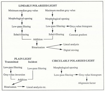
Fig. 1. Flow chart of automated textural analysis of thin-section images. Recordings in linearly polarized light are used in the analysis of ice grains, images in plain light (transmitted and incident) for the analysis of pores.
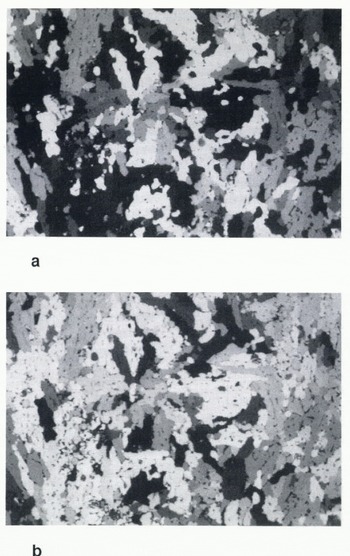
Fig. 2. Thin section of mixed columnar granular ice from 60 cm depth in a core sampled at 66 °8′ S, 05 ° 10′ W on 16 October 1989 in the Weddell Sea (for detailed description of textural classes see Reference EickenEicken and Lange (1991)) recorded between crossed polarizers. These and subsequent thin-section scenes (Figs 4, 6, 7 and 9) measure 50 mm at the base. At the left (Fig. 2a), polarizers are oriented such that the median grey value of the image is at its minimum; at the right (Fig. 2b), it is at its maximum (see also grey-value histograms in Figure 3).
2.1 Basic Hardware Components
Preparation and recording of samples took place in a glaciological laboratory at −25 ° to −30 °C. Thin sections, mounted on a glass slide without a cover, were placed on a universal stage (Rigsby stage) that allowed stepwise rotation of samples and polarizers. A Hamamatsu C2400 cathode ray tube (CRT) camera was employed in image scanning. The advantages of this camera system include high resolution (resolution index of 700 lines), high stability of images and low geometric distortion (< 1%), Beside control of gain and offset, CRT voltage can be compensated locally across the screen in order to remove artificial grey-value gradients, especially for recordings made in plain light. As is often the case in size analyses performed with video systems, artificial compression of the image due to deviating camera/image-board standards has to be corrected, either by accounting for the appropriate correction factor in linear analyses (in most systems between 1.2 and 1.5; cf. section 2.5.2) or through geometrical rectification of the image for non-linear filtering (cf. section 2.5.3).
Image digitization was performed by a Matrox PIP-1024B image-processing board installed on a Compaq 386 microcomputer clocked at 20 MHz (for a detailed description refer to Reference Perovich and HiraiPerovich and Hirai (1988)). The board resolves grey values from 0 (black) to 255 (white) for images composed of 512 by 512 pixels. Utility features of the board include a variety of digital filters based on a mask size of 3 by 3 pixels, performed in few seconds’ time. Because image data are relatively voluminous (e.g. 4 images occupy 1 megabyte of memory), the hard disk suffices for intermediate storage only. Data are archived on an optical disk drive which combines the advantages of a high-data-density medium with those of quick access to individual files.
2.2 Steps Taken in Preparation of Textural Analysis
2.2.1 Sample Preparation
It is important in textural analysis to achieve as high a quality of input image as possible. Emphasis has therefore been placed on careful sample preparation. Thin sections are cut so that they can be microtomed and polished from both sides in order to ensure a smooth surface devoid of artificial grooves (cf. Reference EickenEicken and Lange, 1991). Final section thickness amounts to approximately 0.5 mm.
2.2.2 Recording and Digitization of Images
When a thin section of ice is placed between crossed polarizers, individual grains appear in different colours and shades. This is due to the fact that, when entering an ice sample, a wave of linearly polarized light breaks up into two components travelling at different speeds (birefringence). When leaving the birefringent medium, the component rays display a characteristic phase lag. Upon recombination in the upper polarizer above the sample, some wavelengths are filtered out of the original beam of white light by destructive interference — the crystals appear coloured. The exhibited colour depends on the two factors that determine the phase lag between the waves. In this case these are the section thickness and the tilt angle of the optic axis which for ice coincides with the crystallographic caxis. Crystals exhibit no birefringence in propagation directions parallel to their optic axes. With increasing tilt angle and decreasing section thickness, so-called higher-order interference colours give way to orange and grey of increasingly darker shade (for a more precise and comprehensive account consult, for example, Reference Gribble and HallGribbley and Hall (1985)). Crystals with vertically oriented taxes appear completely dark.
Apart from displaying characteristic interference colours, anisotropic crystals appear in different shades as the orientation of the crystal changes with respect to the planes of polarization. If the horizontal projection of its caxis, i.e. the azimuth, corresponds to either plane of polarization, a crystal appears completely dark (maximum extinction). At angles of 45 ° between the polarization plane and the c-axis azimuth, minimum extinction corresponding to a grey-value maximum occurs. Consequently, the grey-value distribution of an image consisting of an assortment of crystals varies as the orientation of the thin section with respect to the polarizers. Thus, samples such as the one featured in Figures 2 and 3 appear quite dissimilar when viewed under different polarizer orientations and have to be recorded in a normalized fashion for consistent, comparable results. This problem can be solved by recording a thin section twice, such that one image exhibits the minimum and the other the maximum median grey value G md(min) and G md(max) displayed by the sample (Figs 2 and 3). These two different orientations of the polarizer/ analyser pair are easily determined interactively when recording a sample and relocated at a later stage because they are singular and invariant with regard to different recording conditions. The difference
contains information on the degree of crystal-optical alignment of the sample (not considering possible artifacts due to equivocal mapping of colours into grey tones). The larger D, the larger the degree of caxis alignment (Fig. 3). For crystals with randomly distributed caxes, Dapproaches 0. The highest degree of alignment corresponds to a value of Dachieved for a single crystal extending over the whole field of view. The angle between the two orientations of polarizer/analyser during recording ideally (i.e. in the case of preferred alignment) measures 45 °. Analysis of grain shape is eased by ensuring that the rows and columns of an image are aligned in parallel with the vectors of polarization. If this is the case, the same is true on average for the elongation axes of crystals, since caxes of ice crystals are oriented at right angles to the basal plane which coincides with the tabular morphology of grains.
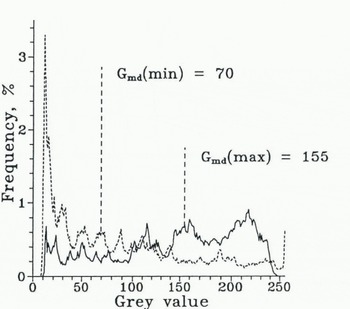
Fig. 3. Grey-value histograms of the sample depicted in Figure 2, recorded at the two orientations of polarizer/analyser for which the median grey value Gmdis at its minimum and maximum, respectively.
In addition to pictures taken in linearly polarized light, the sample is also recorded in circularly polarized light with the aid of two λ/4 plates placed between sample and polarizers. In circularly polarized light, any shading of crystals due to their orientation with respect to the plane of polarization is removed because the electro-magnetic field vector rotates about the axis of light propagation. Hence, only the tilt of crystals’ caxes and section thickness are expressed in the grey-value distribution (cf. section 2.3).
The recordings in plain light supply the basis for studies of sample porosity. As a ray of ordinary light passes through a medium, it is refracted or reflected by internal phase boundaries. As a result of internal scattering and absorption, pores appear dark in ice thin sections with a bright background (Fig. 4a). This effect is more pronounced for gas than for liquid inclusions because the difference in refractive indices with respect to ice, which determines the limiting angle of internal reflection, is larger for the former. Illuminating a sample merely from the sides over a dark background causes pores to appear as bright speckles in a matrix of dark ice due to the same phenomena (Fig. 4b). Before the recording and digitization of these two images, artificial grey-value gradients resulting from uneven lighting, etc. are removed through the accentuation with the aid of false-colour look-up tables (LUT) and subsequent local compensation of CRT voltage.

2.2.3 Filtering Images in Preparation for Analysis
Pores may appear as dark speckles due to internal scattering and absorption in images recorded between crossed polarizers. This is particularly true for grains with internal inclusions recorded at orientations of minimum extinction, as is evident in the example shown in Figure 2b. Here, pores might erroneously be interpreted as small crystals by the grain-boundary identification algorithm. To minimize these errors, images recorded between crossed polarizers are subjected to non-linear filtering routines prior to analysis.
Since non-linear filters are also used for the determination of size distributions as described below, an illustration of this technique and other local transforms employed in the analysis is appropriate. Essentially, the method consists of translating a mask (B) of a given size pixel by pixel across the features (A) of an image (Fig. 5). For each position of the kernel B, the pixel that is currently at the origin (in this case the centre) is set to either the maximum or minimum value of the set of pixels covered by the whole of B. The former convolution is referred to as dilation (expressed through the symbol ⊕), as it expands high grey-value objects in the image (Fig. 5). The resulting image represents the union (denoted by U) of features (A) with the translated elements (b) of the kernel B (Reference SerraSerra, 1982):
The latter convolution is termed erosion (expressed through the symbol ⊖) resulting in the shrinking of high grey-value features. It corresponds to the intersection (denoted by ∩) of A with the translated elements b of Β (Reference SerraSerra, 1982);
The process of sequentially dilating and eroding an image is referred to as a morphological opening (Reference SerraSerra, 1982):
where BTis the reflection of Β about the origin; here, BT= B. By morphologically opening an image with a mask of size 2b + 1, all features smaller or equal in size to 2b and exhibiting lower grey values than their surroundings will be removed.
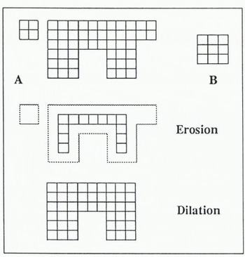
Fig. 5. Schematic representation of the morphological opening of a set of two dark objects (denoted A) with a quadratic mask (denoted B) by performing an erosion-dilation sequence.
Opening the images of sea-ice samples recorded between crossed polarizers with masks 5×5 pixels in size proved to remove the majority of signals, i.e. more than 90%, resulting from pores within grains. This is illustrated in Figure 6 which represents the image of Figure 2b after the morphological opening. Errors introduced into automated grain-boundary recognition through misinterpretation of inclusions can therefore be kept to a minimum. For samples with larger pores, e.g. glacial ice, larger masks have to be employed for the morphological opening. It has to be taken into account during textural analysis that the morphological filters employed might efface crystal features up to 2b in size. This is noticeable in Figure 6 as a slight blurring of outlines. For specimens with inclusions as large as the crystals, the method obviously fails altogether.
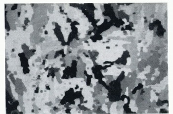
Fig. 6. Sample depicted in Figure 2 after morphological opening with a mask 5 by 5 pixels in size. Note the disappearance of intraeranular bores.
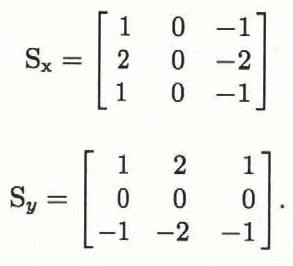
The second step in image preparation consists of low-pass filtering all frames recorded to remove high-frequency noise generated by the camera or the analogue/digital(A/D)-converter, thereby improving the efficiency of grain-boundary recognition algorithms. The image S(x,y)is convolved with a 3 × 3 kernel h(u,v)such that the resulting picture Sprime(x,y)is given by:
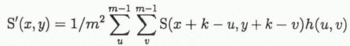
with m = 3, k = (m− 1)/2, (x, y) and (u, v)being the coordinates of picture and kernel elements, respectively (Reference HaberäckerHaberäcker, 1985). For low-pass filtering, the kernel is specified by the matrix
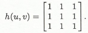
As a result, pixels are set to a value that corresponds to the average of all nine elements covered by the mask.
2.3 Grey-Value Analysis
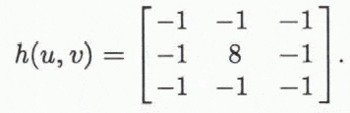
Prior to the identification of grain boundaries, the spatial grey-value contrast inherent in an image is described by the contrast gradient (CG). CG serves as an integral measure of the grain-boundary density and the degree of crystal-optical alignment of a sample. Details of the definition and the determination of CG have been described in Reference EickenEicken and Lange (1991). Essentially, the grey-value gradients across the image are accentuated by application of a Laplacian transform:
From the grey-value histogram of the resulting image, CG is computed by fitting a straight line of slope sto the lower half of the curve and computing CG according to
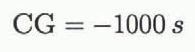
such that the range of values encountered for typical ice samples ranges between zero and 10. High values of CG imply high grain-boundary densities and a low degree of crystal-optical alignment within a sample, and vice versa. Determining the so-called alignment factor (AF) in analogue to CG for images recorded in circularly polarized light provides information about the tilt of grains’ caxes, AF being low for samples with horizontally oriented caxes.
In sea-ice studies, one may often observe the textural sequence: (1) fine-grained, no alignment; (2) coarsegrained, little alignment (caxes tending into the horizontal plane); and (3) coarse-grained, pronounced alignment (one-point maximum within the horizontal plane) after the onset of ice growth (Reference Weeks and AckleyWeeks and Ackley, 1982). Here, contrast gradient and alignment factor are of use because they suffice as descriptors of this sequence, distinguishing between all three growth stages. Importantly, the determination of CG and AF is completely independent of notions or preconceptions about the definition and identification of grains and grain-boundaries.
2.4 Segmentation of Images: Distinguishing Ice from Pores, and Grains from Grain Boundaries
2.4.1 Grain Boundaries
Image segmentation is aimed at identifying grain boundaries in images recorded between crossed polarizers or identifying pores in images recorded in plain light. Since identification of grains or grain boundaries is a prerequisite to determination of the majority of textural parameters, segmentation is of considerable importance in automated textural analysis. If we assume that a grain in the broadest sense can be perceived as a domain of homogeneous crystal-lattice orientation (possibly including other phases), then the process of segmentation consists of the identification of (1) foreign component phases, which have to be analysed separately, and (2) domain boundaries. Item (1) has been taken care of by image-preparation algorithms described in the previous sections. With regard to (2), image analysis of thin sections can at best yield information on crystal-optical rather than crystallographic orientation of domains. In the majority of cases, however, this information suffices completely.
Grey-tone recordings access only a fraction of the full information inherent in a thin section exhibiting interference colours higher than the first order. Difficulties resulting from this shortcoming can be resolved by cutting sections to a final thickness corresponding to low-order white interference colours. Alternatively, one may assume that no significant information is lost when taking grey-tone recordings of coloured sections. The significance of this information loss is covered in section 3.1, for now the latter assumption shall suffice.
Two approaches were taken to devise an algorithm that identifies grain boundaries by evaluating the grey-value distributions of images taken between crossed polarizers. Whereas one is fairly elaborate and yields information on the crystal-optical orientation of phases by analysing sequences of images recorded under varying orientations of polarizers (cf. Reference EickenEicken, 1991), the other, presented below, is simple and has been proven to yield satisfactory results even for samples of complex texture (Reference EickenEicken and Lange, 1991). The latter algorithm recognizes grain boundaries as locally confined zones of high contrast, achieved by Sobel-filtering of both images taken between crossed polarizers as a first step (i.e. with minimum and maximum median grey value, see Figures 2 and 3). This convolution computes grey-value gradients in x- and y-direction with kernels hx and hy defined as (Reference HaberäckerHaberäcker, 1985):
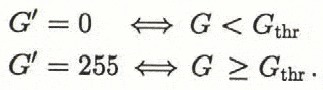
Thus, high grey values are assigned to regions of high contrast and vice versa. By adding both convoluted images (and setting all values >255 to 255), information about image contrast is combined for the two singular polarizer orientations. The resulting image is binarized about a threshold Gthr with each pixel Gbeing assigned a new value of G′ of either 0 or 255, so that
An example of this segmentation procedure is given in Figure 7 for the sea-ice sample introduced above. Dynamic determination of the threshold, such that it corresponds to a given areal fraction of grain boundaries in the image, as suggested by Reference Russ and RussRuss and Russ (1987) and other authors, is of little value in this case because the grain-boundary density varies considerably between samples. Consequently, the threshold has been fixed at a static level that corresponds to the minimum grey-level fluctuation attributed to a grain boundary. It is assumed that all values below the threshold are associated with intragranular phenomena (undulose extinction, sub-grains, etc.) which are not considered in the segmentation process (an estimate of the errors resulting from this approach will be discussed in section 3.1). Based on analysis of both glacial and sea-ice samples, G thrhas been set to 128 for our studies.
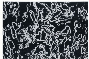
Fig. 7. Sample depicted in Figure 2 after the segmentation process (black: grains; white: grain boundaries).
2.4.2 Pores
The distinction between pores and grains is best made by evaluating the images recorded in plain light. As discussed above, pores appear dark in plain transmitted light due to internal absorption (Fig. 4a). The same physical cause has the adverse effect when light is shone through a sample in narrow beams from the sides only; pores appear as bright speckles in a dark matrix (Fig. 4b). In principle, two approaches can be taken to segment images. Either spatial contrast along the perimeter of inclusions is used to determine pore boundaries, or pores and ice are distinguished by their differences in grey value. For the samples analysed in this study, the first approach does not lead to convincing results. Grey-level contrast within inclusions can be so high as to render correct identification of pore boundaries impossible (such as in groups of pores in the lower left corner of Figure 4a and Figure 4b). Further difficulties arise as the changes in grey value between crystals and pores often appear as gradual transitions owing to scattering in the boundary zone.
Segmentation through binarization of images, based on a grey-value threshold to distinguish between crystals and pores, holds more promise. The grey-value histogram of the example of a sea-ice thin section recorded in transmitted plain light is shown in Figure 8. The pronounced peak at high grey values corresponds to the ice, whereas the drawn-out tail represents pores. Where is one to fix the threshold G thrthat separates crystal and pore fraction in the histogram? The lack of any self-evident division is due to the gradual grey-value transition that characterizes pore boundaries. Here, not even interactive manual setting of thresholds is warranted to yield reproducible results. Determination of Gthr is computed from the magnitude of the median grey value Gmedof the entire image’s grey-value distribution. Here, a quadratic equation with empirically determined coefficients has been employed in estimating Gthr:
Comparison with manually segmented images shows that this approach yields satisfactory results, while ensuring independent, objective analysis of samples. Results are improved significantly by combining the two images recorded in plain light before binarization about Gthr-The binarized image, based on Figure 4a and Figure 4b, is shown in Figure 9. The entire segmentation procedure comprises these steps: (1) inversion of the image recorded in plain light such that each grey value G0is replaced by Gn= 255 − G0, (2) addition of the two images with all grey values > 255 set to 255, and (3) binarization about a threshold Gthrsuch that all grey values < Gthrare set to 0 (ice) and all others to 255 (pores), Gthrbeing determined according to Equation (7).
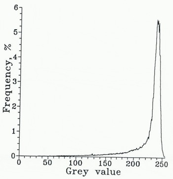
Fig. 8. Grey-value histogram of the plain-light image shown in Figure 4a. The peak at high grey values corresponds to the ice phase; pores are represented by the lower end of the spectrum.
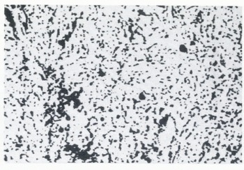
Fig. 9. Sample depicted in Figure 4 after the segmentation process (black: pores; white: ice; porosity ApA= 24%, mean chord size cm= 0.4 mm J.
2.5 Extracting Textural Parameters from Segmented Images
2.5.1 Determination of Porosity and the Effect of Finite Section Thickness
Stereologically, one of the simplest parameters to extract from an image segmented into ice and pores is the fraction of the total area covered by pores APA From Reference DelesseDelesse (1847; cited in Reference WeibelWeibel, 1979) we know that porosity VPV is given by the simple formula:
provided there is a uniform distribution of pores in the direction normal to ΑPA . Unfortunately, a thin section of 0.5 mm thickness with pores down to a few tenths of a millimetre in size bears little resemblance to the ideal concept of a planar, truly two-dimensional sample. Thus, in practice, we are not determining APA but rather the projection of the porosity VPV into the plane of vision (Fig. 10).
In order to account for this artificial increase in VPV by sampling from a volume of thickness t, one can correct determinations of ΑPA with a compensating factor Kt (Reference WeibelWeibel, 1980):
Kt is a function both of tand the size of inclusions (which in this case are assumed to be uniform in size). For spherical pores of diameter d, one obtains
The porosity determined on a section of, for example, 0.5 mm thickness with pores of diameter 1 mm would then be too high by a factor of 1.75. The pore geometry of sea-ice samples, in particular, is of such complexity as to necessitate a more thorough treatment of issues relating to section-thickness effects (see also the instructive monographs by Reference WeibelWeibel (1979, Reference Weibel1980)). As the grain-size of glaciological samples typically ranges one order of magnitude above the thickness of thin sections, correction of the thickness effect for grain-size determinations was deemed unnecessary.
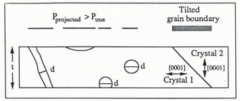
Fig. 10. Effects of finite section thickness, with pores from the entire volume projected on to the video image with a resultant overestimation of porosity. Note that pore size will be underestimated for spherical pores because of truncation. Inclined boundaries between crystals may induce interference fringes or feign abnormally broad grain boundaries.
2.5.2 Linear Analysis: Textural Parameters Obtained from Test Lines Intersecting with Grains or Pores
Principally, linear analysis consists of extracting the lengths of lines intercepting features within a sample (Reference WeibelWeibel, 1979). Here, we consider intercepts of horizontal and vertical lines, i.e. rows and columns of the digital image, with grains or pores. Ideally, these test lines should be randomly distributed. However, such random sampling has to rely on elaborate interpolation schemes when working on orthogonal digital grids. The concept for textural analysis of glaciological samples presented here does not justify these procedures, even more so, because the digitization procedure ensures that the mean crystal-optical orientation of grains is parallel to the frame’s principal axes (see section 2.2.2). On average, this procedure precludes that horizontally elongated grains or pores (e.g. columnar crystals or brine layers) are aligned at 45 ° with respect to the image’s reference frame (see, for instance, Figs 2 and 4).
A simple, albeit powerful stereological descriptor, the grain-boundary or perimeter density ΒA follows immediately from the number of chords Νextracted from a binarized image of area Aand resolution b(expressed by a pixel’s lateral dimension) according to
Thus, BA describes the length of grain perimeters or boundaries per unit area. Samples composed of small or highly tortuous grains would consequently exhibit relatively high values of ΒA . Though computation of this parameter is straightforward, the implications of resolution and orthogonal geometry of the digital image entering into the equation are much less so. From a crystallographic viewpoint, and depending on the characteristics of a given sample (e.g. distribution of other phases, direct impingement of grains), ΒA may have to be modified by an appropriate “internal-surface” factor. The even simpler point-count measure PA of the boundary density, as given by the number of pixels per unit area belonging to grain boundaries, is not considered here. Since it does not strictly depend on the grain’s surface area but also on the width of the boundary zone, it corresponds essentially to porosity ΑPA which can also be viewed as a pixel measure of “boundary space” per unit area.
The statistical descriptors of the intercept or chord-length distribution f(ci)(illustrated for the sea-ice example in Figure 11), i.e. its mean (Cm), standard deviation (σ)and skewness (f), represent another set of useful textural parameters. They are defined as (Reference LloydLloyd, 1984)
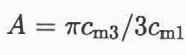
Whereas Cm describes the mean grain-size of a sample, fis a measure of the asymmetry inherent in an intercept distribution. For f< 0, the curve is skewed towards lower values than the normal distribution; for f> 0, it tails towards higher values. As has been shown, fcan be used in automated discrimination between different sea-ice textural classes (Reference EickenEicken and Lange, 1991). The analysis of chord sizes does not take into account the location of intercepts within an image nor does it identify the set of chords that constitute an individual grain. This circumstance may be viewed both as a great advantage and a serious shortcoming of linear analysis in general. It can be quite disadvantageous in some studies not to consider individual grains, and not to record their sizes and shapes one by one. Yet, facing complex textures (as in the case of sea ice), one of the strengths of linear analysis is that it does not require the identification of individual grains, which, for stereological reasons, can be associated with a large error, no matter whether performed automatically or manually. Even so, grain-sizes can be computed from the chord-size distribution. As shown by Reference CroftonCrofton (1868) and Reference DaviesDavies (1962), the mean area Aand mean perimeter Βof features with convex outlines are described by the first and third moment Cm1 and Cm3 of the chord-size distribution according to
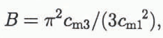
with the kth moment defined as
Typical values computed from an example of a chord-size distribution are indicated in the caption to Figure 11.
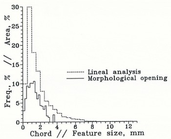
Fig. 11. Chord-size distribution of the example of sea ice shown in Figures 2, 6 and 7 as obtained through linear analysis (mean chord size Cm= 1.8 mm, σ = 1.5 mm, f = 3.4, computed mean grain area A = 18 mm2, computed mean grain perimeter Β = 32 mm; see section 2.5.2 for further explanation of symbols and parameters). Also shown is the feature-size distribution determined through morphological opening.
The parameter I, which has been defined as the ratio between mean chord sizes determined along each of the image’s two principal axes, describes the mean elongation of grains. Isometric grains correspond to I− 1, whereas for elongated grains I< 1. More elaborate measures of grain geometry, such as boundary curvature, can be extracted from the chord-size distribution based on the relations given by Reference DeHoff and EliasDeHoff (1967).
2.5.3 Morphological Filters as Digital Sieves
In order to overcome the restrictions of linear analysis outlined above and to come closer to describing the “true” grain-size distribution, morphological filters were relied on to extract information on the size distribution of cross-sectional areas displayed in a thin section (see Figure 11 for the corresponding example). As outlined in section 2.2.3 and Figure 5, the morphological opening can be quite effective in removing low grey-value features from an image. By applying a sequence of openings with increasing mask size to the binarized image with delineated grain boundaries, features of increasing sizes are extinguished. For each step, the areal fraction (ΑA)of features removed during individual openings is recorded (Fig. 5; cf. Reference SerraSerra, 1982).
By referring to areal rather than numerical density, the peaks at low intercept lengths typical for chord-size frequency diagrams are not evident in morphological analysis, in which more weight is given to larger features (Fig. 11). As it has been described here, the digital sieve does not distinguish between individual particles or entities as does its hardware prototype, but considers grains and grain protrusions as equivalent (Fig. 5). Analysis of grain-sizes requires identification and enumeration of grains as discussed below. The similarity between the distribution of chords and morphological sizes typical for granular ice samples is mostly due to stereological factors (cf. Fig. 11).
2.5.4 Automated Enumeration of Features
Similar to point-density methods discussed in section 2.5.2, one can determine the density of grains NA per unit area in a thin section. This has been achieved here by using an algorithm that automatically identifies all sets of pixels bounded by closed curves, assuming these are individual grains. ΝA is easily determined by simply counting grains manually or by using a semi-automated system after manual tracing of grain boundaries. Errors can result if different cross-sections of a single, not fully convex grain are interpreted as individual crystals (Fig. 12). This stereological problem of two-dimensional sampling of three-dimensional structures has been discussed by Reference RigsbyRigsby (1968) and Reference HookeHooke (1969) for glacial ice. Experience shows that the problem may be of equal or higher importance in the study of sea ice (see, for instance, the concave grains in Figure 2). However, automated techniques are prone to substantial errors of a different kind. In cases where contrast between adjacent grains is low (either because the lattice mismatch between crystals is very small or because of video-recording conditions), the segmentation algorithm might not completely identify the boundary, leaving the grain bounded by an open curve. This is schematically shown in Figure 12, but it is also evident in our example with highly aligned grains and sub-grains visible (Fig. 2b, bottom left). In the corresponding segmented image (Fig. 7), grain boundaries cannot be fully traced in this area. As a consequence, the counting algorithm will consider adjacent grains connected through a perforated boundary as one crystal. Whereas this does not represent a problem in linear analysis, for example, where the chord-size distribution is not particularly affected, these small perturbations prove to be a source of larger errors in the automated enumeration of grains. Thus, an image consisting of tens of grains with boundaries properly identified except for one pixel within each boundary would be counted as one crystal (Fig. 12), although parameters such as the grain-boundary density would deviate by a fraction of a per cent.
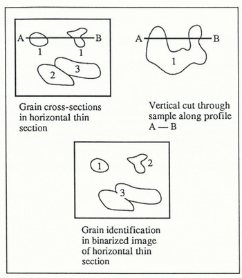
Fig. 12. Distribution of grain cross-sections in a horizontal thin section and for a vertical cut (upper left and right), and identification of grains through automated analysis (crystal 1 regarded as two grains, crystals 2 and 3 as one grain due to incomplete segmentation).
2.5.5 Edge Effects: Correcting for Truncation Errors
Features located near the margins of an image are likely to be truncated by the boundary. This circumstance has to be taken into account for size determinations, either by disregarding clipped grains in the course of the analysis or through later correction of the resulting data. The first option holds most promise for operations such as enumeration of grains or pores by counting only half of all features cut by the image margins. In chord-size analysis, a similar approach was taken by placing a frame within the image and considering only chords whose centre points fall within this frame. The width of this boundary zone is determined by the largest feature present within the sample. Restrictions are placed on this method by elongated grains cut at an oblique angle. Alternatively, intercept data have also been corrected after determination according to a method suggested by Reference Hougardy and StienenHougardy and Stienen (1978). Here, the true length of truncated intercepts is computed from the chord-size distribution of individual rows and columns.
In general, the problem of edge effects is intricately linked to the problem of sampling errors. The more features that are recorded within an image, the less important is the artificial reduction in, for example, mean intercept length due to truncation. Truncation significantly alters results only as the grains or pores recorded become very large compared to the image size. In cases where constrictions with regard to core diameter, etc. do not allow for larger samples, it also becomes increasingly difficult to quantify truncation errors reliably. Ultimately, the problem may be resolved either through a sufficient sampling density or possibly by relying on textural parameters, such as grain-boundary densities, that are not subject to truncation errors.
2.5.6 Computing “True” Pore- or Grain-Sizes from Chord-Size Distributions
When sampling along test lines arranged on a sampling plane, the parameters obtained through linear analysis, such as mean chord size, will underestimate the true feature size, assuming that the objects are of spherical or near-spherical shape. Planar cuts through grains or pores will mostly generate smaller-than-maximum cross-sections, whereas the test lines will mostly miss the centre points of an object. Of the various correction procedures that have been devised (cf. Reference WeibelWeibel (1980) for a detailed description), the method of Reference Cahn and FullmanCahn and Fullman (1956) is particularly useful in chord-size analysis. They determined the number of chords n(c)dc with lengths between cand c-dc to be
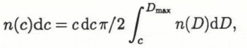
where n(D)dDis the number of spherical particles between Dand D-dDin diameter. For discrete intercept lengths as obtained from digital analysis, Reference BockstiegelBockstiegel (1966) derived a solution to the equation yielding the number of spherical particles ![]() between
between ![]() and
and ![]() in diameter:
in diameter:
According to Bockstiegel’s method, three-dimensionally valid grain-size distributions have been computed for c. 50 representative samples of granular ice composed of convex, isometric grains (both glacial and sea ice). In many cases, nonsensical size distributions with negative or abnormally high frequencies resulted; almost all computed distributions did not correspond to the true picture. The most obvious explanation for this inexactitude, which has also been reported by Reference AlleyAlley (1987) for semi-automated analysis of firn samples, would be differences in the assumed and actual sample geometry. The method is bound to fail when applied to textures comprising indented, non-spherical grains, which are frequently observed in sea-ice studies (cf. Fig. 12). Yet, even for particles almost spherical in shape, part of the explanation is associated with the very principles of automated digital analysis. The approximation of comparatively small features within an image by orthogonal picture elements is rather unrealistic and results in abnormal distributions of small chord sizes. It could be argued, however, that the information gained from three-dimensionally valid size distributions is generally marginal, especially when considering the effects of resolution and analysis procedure on the outcome. Thus, it appears most appropriate to restrict computation of derived parameters to cases where they are specifically needed for analysis and where all significant errors involved in the computation can be quantified.
3 Discussion
3.1 Errors in Automated Image Processing of Thin Sections
Automated analysis allows for the extraction and evaluation of large quantities of data. Consequently, sampling errors with regard to obtaining a statistically sound sample of, for example, chords or pixels from a specific region (i.e. an image) are generally rather low. Since the level of statistical significance of such a data set is proportional to n−½ and the number of observations n(e.g. the number of chords) is typically >104for the materials studied, data obtained through linear analysis correspond to significances well below the 0.01 level (cf. Reference LloydLloyd, 1984). In contrast, the error involved in obtaining a thin section that is representative of the body of the ice under investigation can be considerable.
Errors due to instrumentation have been studied in detail (Reference EickenEicken, 1991) and were only of minor importance with the hardware implementation described in section 2.1. If emphasis is placed on a camera system that yields stable images of low geometric distortion and neither sample nor camera are tilted against the optic axis of the recording stage, the resulting errors in determination of mean chord size are < 1%. A/D-conversion errors of the video signal can be substantial; yet, they are of interest only in the study of grey-value distributions of individual pixels (cf. Reference EickenEicken, 1991).
Errors due to the method of analysis are of greater importance. Some of these, such as digitization or edge effects have already been discussed in the preceding sections. The most significant errors, however, originate from incomplete or faulty segmentation of images, and are directly or indirectly related to one of these five sources: (1) intragranular pores are mistaken for grain boundaries, (2) interference colours of differently oriented crystals are mapped into the same grey value upon digitization, (3) contrast between neighbouring grains is extremely small due to sub-parallel alignment of grains, (4) adjacent crystals with the same c-axis tilt exhibit the same grey value because caxes are either symmetrical about the plane of polarization or orthogonal to one another, (5) interference fringes displayed by grain boundaries are mistaken for individual grains.
The morphological opening of images in preparation for analysis minimizes errors in connection with source (1). Interference fringes (source (5)), which appear in thicker sections or in cases where grain boundaries are more or less parallel to the section plane over greater distances, have been rarely observed. More common, however, are grain boundaries that are artificially widened because of overlapping grains (schematically shown in Figure 10, some of the broader grain boundaries apparent in Figure 7 may also stem from this cause). Due to their high spatial contrast, these features are nevertheless mostly taken to be part of the grain boundary and will at worst yield a small size reduction of intercepts drawn across the respective grain.
Common to sources (2) to (4) is that they result in incomplete identification of grain boundaries. For all samples analysed, the orthogonal or symmetrical alignment of caxes of neighbouring grains has only been encountered occasionally (source (4); cf. Reference EickenEicken, 1991). The transformation of different interference colours into the same grey value, on the other hand, is one of the commonest sources of error in grey-tone analysis; it is virtually impossible to quantify or to correct for in the analysis. Nevertheless, one can minimize this element of bias during the preparation and recording of samples. Thus, sections should be cut to such a thickness as to avoid the co-appearance of interference colours that are transformed to similar grey values. Information about the colour sensitivity of the camera system can easily be obtained through digitization of standardized colour maps.
Sub-parallel alignment of adjacent grains (source (3)) may lead to incomplete grain-boundary identification as the contrast drops below the response level of the segmentation algorithm. Comparisons between automated segmentation and determination of c-axis orientation for adjacent crystals showed that for angles of c-axis mismatch of less than 5–10 °, detection of grain boundaries is incomplete (Reference EickenEicken, 1991). In some cases, segmentation may have to be either based on automated determination of crystal-optical orientation or abandoned altogether and replaced by alternative methods such as the contrast analysis described in section 2.3. This problem is important in the study of columnar sea-ice samples because the alignment of caxes can be so high as to blur any distinctions made between grains and sub-grains (see also Figure 2b and the pertinent comments made in section 2.5.4).
Even though it is difficult at this stage to quantify the relative contributions of the sources of error discussed above for a general case, it appears that further work would have to concentrate on improvement of image segmentation. Yet, such shortcomings of automated techniques in identifying crystals and grain boundaries may reflect fundamental problems, which could also pose difficulties during manual determination (as in the case illustrated in Figure 2). Here, automated texture analysis might supply the impulse for a closer theoretical examination of the matter.
3.2 Automated Image Analysis of Thin Sections in Glaciological Studies: Concluding Remarks
Automated image analysis of sea-ice or glacial-ice thin sections calls for methodical developments that differ from those intended for the study of snow or firn. In this paper, I have tried to outline a procedure for efficient textural quantification that is both simple and easily implemented, relying on an inexpensive image-analysis board installed in a microcomputer. The technique results in efficient characterization of samples in a reproducible, objective manner. This is of particular interest in studies which call for detailed comparisons between larger amounts of data.
Automated grain-boundary identification based on an algorithm that responds to image contrast is quite successful as a precursor to linear and morphological analysis of samples. Limitations imposed on the system, which render automated enumeration of crystals more difficult, are connected either to the problem of transforming interference colours into grey tones or to incomplete identification of low-angle grain boundaries. Whereas the former problem is one of instrumentation or sample preparation, the latter is also concerned with the definition of grain boundaries and their manifestation in thin sections. Currently, we are aiming at an evaluation of different segmentation algorithms through extraction of the full crystal-optical information inherent in a thin section to come to terms with these issues. In the analysis of pores, further work would need to concentrate on the stereological issues relating to finite section thickness and problems of two-dimensional sampling.
The image-analysis procedure, as it has been outlined above, offers the opportunity for evaluation and comparison of a variety of textural parameters, relating to size and distribution both of pores and grains as well as to the crystal-optical orientation of components. The combination of this extensive information could eventually lead to an integrated determination of diverse textural quantifiers and provide a more complete and distinct picture of ice as a material.
Acknowledgements
This work has greatly benefitted from the encouragement of M. Lange. For the enthusiasm transferred to me at the start of this project, I am grateful to S. Ackley and D. Perovich. The comments of two anonymous reviewers are gratefully acknowledged. This is contribution No. 527 of the Alfred-Wegener-Institut für Polar- und Meeresforschung.
The accuracy of references in the text and in this list is the responsibility of the author, to whom queries should be addressed.


