


1. Introduction
The discovery that sections of the West Antarctic Ice Sheet are losing mass to the oceans (Wingham and others, Reference Wingham, Ridout, Scharroo, Arthern and Shum1998; Rignot, Reference Rignot1998; Shepherd and others, Reference Shepherd2018) with significant implications for global sea levels (e.g. Shepherd and others, Reference Shepherd2018) has given practical importance to understanding the evolution of the grounding line – the boundary between the grounded and floating parts – of marine ice sheets. The general problem of the waxing and waning of a marine ice sheet is a time-variant problem involving varying external forcings, the ice sheet's adjustment to these and the interactions between them (e.g. Fyke and others, Reference Fyke, Sergienko, Löfveström, Price and Lenaerts2018). Nonetheless, one can gain some insight into the dynamics by considering the much simpler question of whether, in conditions of constant external forcing, a steady-state marine ice sheet is possible at all, and if so, whether it is stable subjected to small perturbations. Since the original framing of Weertman (Reference Weertman1974), the matter has received continuous theoretical attention (e.g. Chugunov and Wilchinsky, Reference Chugunov and Wilchinsky1996; Hindmarsh and Le Meur, Reference Hindmarsh and Le Meur2001; Schoof, Reference Schoof2007a, Reference Schoof2007b, Reference Schoof2012; Nowicki and Wingham, Reference Nowicki and Wingham2008; Robel and others, Reference Robel, Schoof and Tziperman2014; Tsai and others, Reference Tsai, Stewart and Thompson2015; Robel and others, Reference Robel, Schoof and Tziperman2016; Kowal and others, Reference Kowal, Pegler and Worster2016; Schoof and others, Reference Schoof, Devis and Popa2017; Haseloff and Sergienko, Reference Haseloff and Sergienko2018; Pegler, Reference Pegler2018), principally arising from the contention of Weertman (Reference Weertman1974) that a marine ice sheet cannot exist in steady state on a retrograde bed (i.e. one that deepens towards the ice-sheet interior), a hypothesis that has become known as the ‘marine ice-sheet instability hypothesis’.
The most complete account has been given by Schoof (Reference Schoof2007a, Reference Schoof2011), who, by restricting attention to rapidly-sliding ice stream flow, reduced the problem to an ordinary differential equation. In a later paper, Schoof (Reference Schoof2012) showed that resulting grounding line locations require prograde bed slopes to be stable. While recent work (Kowal and others, Reference Kowal, Pegler and Worster2016; Schoof and others, Reference Schoof, Devis and Popa2017; Haseloff and Sergienko, Reference Haseloff and Sergienko2018; Pegler, Reference Pegler2018; Sergienko and Wingham, Reference Sergienko and Wingham2019) has questioned the instability hypothesis, it remains a widely-accepted description of the higher driving stress ice streams such as those in streams that characterise, for example, the Amundsen Sea sector. Since the original proposition of Mercer (Reference Mercer1968), melt-triggered instability has been frequently invoked to describe the future evolution of sections of the West Antarctic ice sheet, as, for example, do recent descriptions of the future of the Thwaites Glacier basin (e.g. Joughin and others, Reference Joughin, Smith and Medley2014; Feldmann and Levermann, Reference Feldmann and Levermann2015; Cornford and others, Reference Cornford2015; Seroussi and others, Reference Seroussi2017).
The instability hypothesis arises from there being a monotonically increasing relationship between the thickness at the grounding line and the discharge through it. This, in turn, depends on the assumption that the thickness gradient in the momentum equation is large in comparison with the basal gradient. While this is a reasonable description of ice streams flowing over smooth beds offering considerable resistance to the flow, ice streams can experience a variety of frictional resistance at their beds and flow over bed topography that contains a wide range of spatial scales as Figure 1 illustrates. Since surface expressions of shorter scale topography (e.g. several tens of ice thicknesses wavelength) is generally greatly subdued in the surface gradient (e.g. Gudmundsson, Reference Gudmundsson2003), it follows that the basal and thickness gradients must generally be of the same order, and in such a case there is no longer good reason to suppose a monotonic relationship between grounding line thickness and flux, nor a correspondingly simple relationship between basal gradient and stability.

Fig. 1. Characteristics of the Pine Island Glacier and Thwaites Ice Stream region. (a) Magnitude of the surface gradient $\vert \vec \nabla S\vert$ , $S = b + h$
 ; (b) magnitude of the driving stress (kPa) computed as $\tau _d = \rho g h\vert \vec \nabla S\vert$
 derived from the BedMachine Antarctica data set (Morlighem and others, Reference Morlighem2020); (c) surface $S$
 (blue line) and bed $b$
 (red line) elevation along a flowline on Thwaites Glacier (red line in panel (b)).
In this paper, we examine the role of the basal topography in the existence and stability of steady grounding line locations. To do so, we take a scaling approach that assumes that the buoyancy force is small and similar in magnitude to the longitudinal-stress gradient. By doing so, the effect of the basal gradient in the momentum equation then naturally occurs in the lowest order relation between ice flux and thickness at the grounding line, which also supplies the transcendental equation for the steady grounding-line locations, assuming these exist. We also find that, in cases where the thickness gradient at the grounding line is large, our result reduces algebraically to the monotonic dependence of flux on the thickness of Schoof (Reference Schoof2007a). We also consider the stability of the steady-state grounding line locations, and find that this now depends on the basal curvature in addition to the basal gradient and the simple relationship between basal gradient no longer holds. The stability condition that informs the ‘marine ice-sheet instability hypothesis’ no longer generally applies.
2. Model description
The model is the same as that proposed by Schoof (Reference Schoof2007a). Here we provide a brief description. The flow of an unconfined ice stream into an unconfined ice shelf (Fig. 2) can be described by a vertically integrated momentum balance under assumptions of a negligible vertical shear appropriate for ice-stream and ice-shelf flow (MacAyeal, Reference MacAyeal1989)

and

Here $u( x)$ is the depth-averaged ice velocity, $h( x)$
 ice thickness, $b( x)$
 is bed elevation (negative below sea level and positive above sea level), $A^{-1/n}$
 is the ice stiffness parameter (assumed to be constant), $n$
 is the exponent of Glen's flow law, $g$
 is the acceleration due to gravity, $\tau _{\rm b}$
 is basal shear. $g^\prime$
 is the reduced gravity defined as

where

is the buoyancy parameter. $\rho$ and $\rho _{\rm {w}}$
 are the densities of ice and water, respectively, $x_{\rm {d}}$
 is the location of the ice divide (assumed to be $x_{\rm {d}} = 0$
 ), $x_{\rm c}$
 is the location of the calving front and $x_{\rm {g}}$
 is the location of the grounding line. Basal sliding is described by a power-law function

where $C$ and $m$
 are constant parameters.
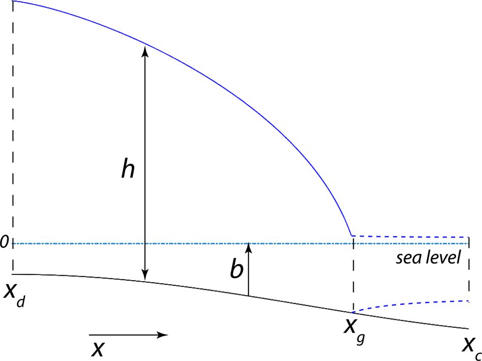
Fig. 2. Model geometry: $b$ – bed elevation ($b\lt$
 0), $h$
 – ice thickness, $x_{\rm {d}}$
 – the ice divide location, $x_{\rm {g}}$
 – the grounding line location; $x_{\rm c}$
 – the calving front location.
The mass balance is

where $\dot a$ and $\dot m$
 are net accumulation/ablation (positive for accumulation) rates of the ice stream and ice shelf, respectively.
Boundary conditions at the divide $x_{\rm {d}}$ and the calving front $x_{\rm c}$
 are
are

and

At the grounding line $x_{\rm {g}}$ the continuity conditions


and

where $\tau = 2 A^{-( {1/n}) }h\left \vert u_x\right \vert ^{( 1/n) -1}u_x$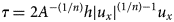 is the longitudinal stress, and the flotation condition

are satisfied. The fact that the ice is grounded upstream of the grounding line and is floating downstream of it is reflected by two inequalities

and

In circumstances where ice shelves are unconfined, the momentum balance of the ice shelf (1b) can be integrated analytically with the boundary condition at the calving front, $x_{\rm c}$ , (6b) and the continuity conditions (7), and the problem can be reduced to the ice-stream part only with the boundary conditions at the grounding line provided by the flotation condition (8) and the stress condition

3. Grounding-line position, flux and stability
In this paper, we wish to study the effect of the basal topography and strength on the grounding line flux and stability. To gain some analytic insight requires us to approximate the model of section 2, which we achieve in this section by supposing the longitudinal stress gradient and the buoyancy to be small parameters. We introduce the characteristic scales for the problem: the bathymetry of a continental shelf $[ b]$ , the length of an ice steam $[ x]$
 and its velocity $[ u]$
 . With these scales, the scales of other parameters of the problem are

and three non-dimensional parameters then emerge. These are $\delta$ , given by (3),

and

where $\varepsilon$ is characteristic of the ice-stream deformation, and $\gamma$
 is characteristic of the ice-stream sliding.
The non-dimensional problem is


and

The behaviour of the system (13) depends on the relative magnitudes of the three non-dimensional parameters $\delta$ , $\gamma$
 and $\varepsilon$
 . In this paper, we will concern ourselves with ice streams for which $\gamma$
 is O(1), describing a flow in which the driving stress and the basal friction are of the same order. Indeed, we will set $\gamma$
 equal to one. Equation (12b) can then be regarded as a constraint on the independence of the three scales; non-dimensionally it insists that the driving stress and basal friction are of the same order. In this and the next section, we will also limit ourselves to situations in which $\varepsilon$
 is small, that is, in which the longitudinal stress gradient is small in comparison with the two other terms of the momentum equation.
There is then finally the choice of the parameter $\delta$ . Numerically, its value is 0.1, and in his treatment of (13), Schoof (Reference Schoof2007a, Reference Schoof2011) took $\delta$
 to be large in comparison with $\varepsilon$
 . This has the consequence that at zeroth order in $\varepsilon$
 , the stress condition at the grounding line (13d) becomes $h$
 = 0 at the grounding line, and the velocity $u$
 becomes unbounded, leading Schoof (Reference Schoof2007a) to introduce a boundary layer solution near the grounding line. As a consequence of the flotation condition, it then follows that the bed depth is also small at the grounding line. We discuss his approximate solution in greater detail in Appendix A. Here, however, we note that this solution is sensitive to the bed topography only through its value at the grounding line, and not, for example, to its gradient and curvature. The alternative, which we explore here, is to take $\delta$
 to be a small parameter of the same order as $\varepsilon$
 , the approach taken by Sergienko and Wingham (Reference Sergienko and Wingham2019) in analysing the corresponding problem when the bed is very weak.
When $\delta \sim \varepsilon$ the terms on either side of the stress condition (13d) are of the same order, and, as noted by Schoof (Reference Schoof2007a), no boundary layer is needed to obtain a solution at lowest order.
3.1. Ice flux at the grounding line
It is convenient to use the flux $Q = UH$ instead of the ice velocity. Taking $\varepsilon \sim \delta \ll$
 1, (13a)–(13d) then become to lowest order


and

To obtain the stress condition (14d) we have used

in (13d). After rearranging terms, and using the momentum balance (14a) to express $H_X$

(13d) becomes (14d), which is the general form of the relationship between the ice flux and the ice thickness at the grounding line. For ice-sheet configurations evolving with time, according to (14b), $Q_X = \dot a - H_T$ , and (14d) becomes

3.2. Steady-state grounding-line ice flux, position and stability
In a steady state, $H_T = 0$ , and the relationship between ice flux and ice thickness at the grounding line (17) becomes

This expression (18) is not new. The same equation can be found in Schoof (Reference Schoof2007a, Reference Schoof2007b) in slightly different guises.
If, at the grounding line, the ice thickness gradient $H_X$ is large in comparison with the bed gradient $B_X$
 in (16), and is also large enough to dominate the velocity gradient in (15), then $B_X$
 and $\dot a$
 may be dropped from (18) to obtain

where $Q_{\rm S}$ is used to distinguish it from (18). This is the approximate solution obtained by Schoof (Reference Schoof2007a, Reference Schoof2011) to his boundary layer problem when $\varepsilon \ll \delta \ll$
 1. (18) provides (19) as a special case when $\dot a$
 and $B_X$
 are small at the grounding line. That the two approaches provide the same algebraic solution is a consequence of Schoof's approximation, which is equivalent to supposing the longitudinal stress is negligible even within the boundary layer. The fact that this approximation is successful even when $\delta$
 is O(1) is a consequence of the non-linearity of the ice flow and the chosen form of the sliding law. This is described in more detail in Appendix A; for our purposes here it is sufficient to note that (18) covers both cases with small and non-negligible basal slopes in the vicinity of the grounding line.
The location of the grounding line $X_{\rm {g}}$ is determined through the addition of a flotation condition to (14). Values of $X_{\rm {g}}$
 are then determined as the roots of the transcendental equation (18) that satisfy the condition (of which there may be none, one or several). When $\delta \sim$
 o(1), the flotation condition (13e), becomes $H = -B$
 to lowest order. We have found, however, that in contrast to (18), this order of approximation does not provide accurate values of $X_{\rm {g}}$
 . Formally, this can be overcome by developing higher order approximations to (13). We have found that while adding considerable algebraic complexity to (18), the additional terms are very small numerically. It is only in determining $X_{\rm {g}}$
 that the increased accuracy in $\delta$
 is needed and we therefore use (18) together with (13e). Physically, this is not surprising. With gentle beds, the location of the steady-state grounding line is very sensitive to the buoyancy.
We now turn to examining the stability of the steady-state grounding-line locations. We use the same approach taken by Schoof (Reference Schoof2012). This is conceptually straightforward, in that we subject the steady states to small, time-dependent perturbations about the steady-state solutions, which we now distinguish with the $\hat{}$ decoration, so that, for example, $X_{\rm {g}}( T) = \hat X_{{\rm g}} + \tilde X_\rm {g}( T)$
 . We substitute such expressions into (14), and by assuming that the time-variant perturbations are small, formulate a linearised perturbation problem. This results in solutions of the form

for the grounding-line evolution. While the resulting problem is an eigenvalue problem for $\Lambda$ , and we are not able to provide a closed form expression for $\Lambda$
 , we can as Schoof (Reference Schoof2012) provide conditions which, if satisfied, ensure all eigenvalues are negative, and as a consequence the grounding-line position is a stable one. The derivation is algebraically complex, and we relegate it to Appendix B. It concludes that provided

and

the grounding line is stable if, and only if,

If the conditions (21) are not met, it is not possible to determine the stability without solving the eigenvalue problem itself. Condition (21a) is met if the stream remains grounded upstream of the grounding line. It is satisfied for any steady-state solution of interest. With $m > 0$ and $\delta < 1$
 , if $B_X( \hat X_{{\rm g}}) \gt$
 0, and the bed is retrograde, then (21b), is satisfied if (21a) is met. On the other hand, if $B_X( \hat X_{{\rm g}}) \lt$
 0 and the bed slope is pro-grade, (21b) must be met independently of (21a) for (21) to be satisfied.
Under the same conditions of small $B_X$ and negligible $\dot a$
 , under which (18) reduces to (19), the only remaining terms in (22) are

on the left-hand side, and $\displaystyle {\dot a( m + 1) Q^{m}}$ on the right-hand side. With (19), (22) reduces to

The left-hand side can be recognised as the derivative of $Q_{{\rm S}}$ of (19), with the flotation condition applied, and so (23) may be written

which is the stability condition determined by Schoof (Reference Schoof2012). Schoof's result is also subject to the condition (21a), but (21b) is a new condition that arises from the additional terms in (18) over those in (19).
4. The effect of bed shape and strength on steady-state configurations
Through supposing $\varepsilon$ and $\delta$
 to be of the same order, section 3 provides expressions for the grounding line flux and stability that acknowledge the role of the basal topography. These expressions are considerably more complex than those that result if the thickness gradient near the grounding line is sufficiently large that the contributions of the basal topography and the accumulation rate to the local strain rate $U_X$
 are small. We might expect that the thickness gradient will increase as the strength of the bed, described here by the parameter $C$
 , increases, and therefore that the significance of the bed topography will become more marked as the bed weakens and the thickness gradient reduces.
In this section, we examine the steady-state grounding line flux and the grounding-line's stability as the bed strength and bed topography are varied, leaving investigations of time-evolving ice sheets to future studies. We examine first the case in which the bed varies only at the scale of the stream length, and then examine the case in which short-scale bed topography is also present.
In this section, we work with dimensional coordinates and variables. In particular, we use the dimensional form of (18), namely

of (19)

of (22)

and of (24)

To validate these approximate solutions, we compare them with numerical solutions of the problem (1), (5), (6), (8) and (10) obtained with the finite-element solver Comsol™ (COMSOL, 2021) that we term ‘exact’, acknowledging their numerical origin. These equations are solved in a steady-state form, that is, $h_t = 0$ in (5). The steady-state solutions are obtained by solving an optimization problem using a minimization procedure based on the Bound Optimization by Quadratic Approximation optimization algorithm (Powell, Reference Powell2009). In all simulations, the grid resolution is spatially variable: it is 200 m through 95% of the length of the domain, and 1 m in the 5% closest to the grounding line position $x_{\rm {g}}$
 .
.
4.1. Long-wavelength bed topography
Figure 3 shows grounding line positions and the corresponding ice fluxes for the smooth, sinusoidal bed shown in Figure 3a for which the maximum magnitude of the basal slope is 1.6$\times$ 10$^{-3}$
 . Each grounding line location corresponds to a particular value of $\dot a$
 , which varies from 2 cm a$^{-1}$
 to 14.1 m a$^{-1}$
 : as (25) implies, the larger thicknesses required at the deeper grounding line locations demand higher fluxes at the grounding line. Figure 3b shows the values of the driving stress and the thickness gradient at the grounding line for a set of grounding line positions and for a range of bed strengths; for $C = 7.6\times 10^6$
 Pa m$^{-1/3}$
 s$^{1/3}$
 (the value used by Schoof (Reference Schoof2007b)) the locations are those shown in Figure 3a. Figure 3b illustrates that the thickness gradient at the grounding line is primarily determined by the strength of the bed, and that with the range of $C$
 we have presented, the thickness gradient ranges from a value of the same order of magnitude as the basal topography (with a maximum slope 1.6$\times$
 10$^{-3}$
 ) to one more than an order of magnitude higher. At the upper end of the range of ice-thickness gradient, we might expect Eqn (26), in which the grounding line flux is a monotonic function of thickness, to be a sufficient approximation. This is confirmed by Figure 3c, which shows flux as a function of thickness, and Figure 3d, which shows the ratio of the numerically computed flux to that predicted by (26). At the higher value of $C$
 , the flux has the monotonic character of (26), but, as the bed weakens, the nature of (25) and its dependence on the bed slope $b_x$
 become apparent, and the grounding line thickness no longer uniquely determines the flux. Nonetheless, the disparity between (25) and (26) is not large: as Figure 3d shows, it reaches only 40% for the weakest bed with (26) consistently overestimating the flux values. Figure 3 also includes a comparison between (25) and ‘exact’ (numerically computed) solutions. In Figure 3a, the ‘exact’ grounding locations are plotted as circles over the locations determined as the roots of (25) plotted as diamonds. The difference between the grounding line positions computed numerically (circles) and as roots of expression (25) (diamonds) ranges from 20 to 920 m as the grounding line location varies from 100 to 800 km. The grounding line positions determined from (25) are significantly more accurate than those obtained from (26) for which the corresponding discrepancies are 3 and 40 km. Similarly, Figure 3c provides the same comparison of the relationship between flux and thickness at the grounding line. It is apparent that (25), and the scale choice that leads to it, provides an accurate approximation of the ‘exact’ solutions.

Fig. 3. Grounding line locations and flux with a smooth bed topography. (a) The grounding line positions for sliding parameter $C = 7.6\times 10^6$ Pa m$^{-1/3}$
 s$^{1/3}$
 and various values of the accumulation; (b) the magnitude of driving stress, $\vert \tau _{\rm d}\vert$
 (kPa) as a function of the magnitude of the ice thickness gradient, $\vert h_x\vert$
 , at the grounding line. Note the logarithmic scale; $\tau _{\rm d}$
 and $h_x$
 are both negative. (c) The relationship between ice flux and ice thickness computed for various values of the accumulation rate $\dot a$
 and sliding parameter $C$
 . The values of $\dot a$
 are discretely chosen, ranging from 2 cm a$^{-1}$
 to 14.1 m a$^{-1}$
 . The size of symbols in panels (a) and (c) correspond to the values of $\dot a$
 . In panels (a) and (c), circles are ‘exact’ solutions, diamonds are the roots of expression (25). (d) Ratio of the numerically computed flux at the grounding line to the one computed with expression (26) derived by Schoof (Reference Schoof2007a).The simulation parameters are the following: bed elevation ${b( x) = b_0 + b_{\rm a} \cos ( ( {\pi x}) /{L}) }$
 , with $b_0 = -500\, {\rm m}$
 , $b_{\rm a} = 250$
 m and $L = 500$
 km; ice stiffness parameter $A = 1.35\times$
 10$^{-25}$
 Pa$^{-3}$
 s$^{-1}$
 (which corresponds to ice temperature $\approx -20^\circ$
 C). In all simulations the ice flow is from left to right in (a).
Turning now to the stability of the grounding line positions, Figure 4a shows the grounding line positions and their corresponding stability as determined by (27). In general, for this smooth bed, (27) is in agreement with (28), the negative bed gradients are sufficient to ensure stability, while the positive bed gradients are sufficient to ensure an unstable grounding line position. However, there is one case, indicated by an arrow in Figure 4a, in which (27) and (28) disagree as to the stability. This is the consequence, in (27), of the terms in $\dot a$ , which peak for the deepest grounding line, coinciding with a grounding close to the largest bed curvature. Here, although on a prograde slope, (27) predicts that the grounding line position is unstable. The accuracy of this prediction is confirmed by an ‘exact’ calculation illustrated in Figure 4b, in which a slight displacement of the grounding line upstream from its steady-state location results in an ongoing retreat.
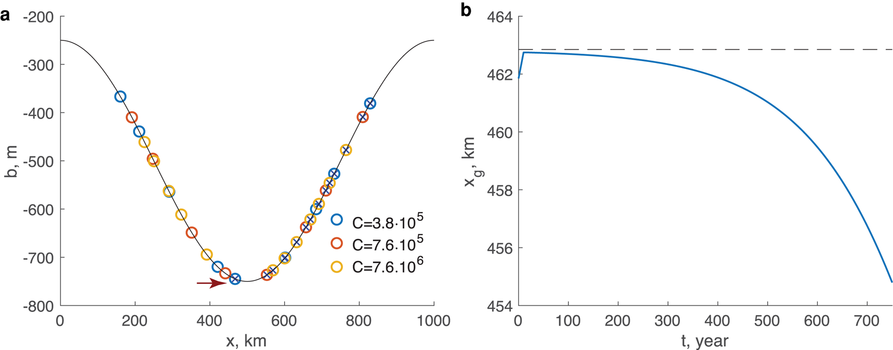
Fig. 4. Stability of grounding line locations with a smooth bed topography. (a) Grounding line positions for various values of $C$ and $\dot a$
 shown in Figure 3c. Open symbols denote stable positions ($\Lambda \lt$
 0), crossed symbols denote unstable positions ($\Lambda \gt$
 0). A red arrow indicates an unstable position that nonetheless satisfies the $q^\prime ( h( X_{\rm {g}}) ) > \dot a( X_{\rm {g}})$
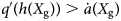 stability criterion (Schoof, Reference Schoof2012), the unstable grounding line position indicated by the red arrow in panel (a). (b) Time evolution of an unstable grounding line position. The steady-state position marked by the black dashed line is for a sliding parameter $C = 3.8\times$
 10$^5$
 Pa m$^{-1/3}$
 s$^{1/3}$
 and an accumulation rate $\dot a = 9.3$
 m a$^{-1}$
 .
.
4.2. Short-wavelength bed topography
The presence of the basal gradient in (25), and of the basal curvature, in (27), suggests that as the length scale of the basal topography shortens, its effects on grounding-line flux and stability will be correspondingly larger. It is the purpose of this section to investigate this hypothesis. To do so, we nonetheless need to limit any shorter scale topography to undulations whose length-scale remains large in comparison with the ice thickness, in keeping with the scale assumptions that underlie (1). Secondly, when short-scale topography is present, the longitudinal stress gradient can be as important as the basal friction and driving stress, in addition, it may no longer be appropriate to drop $B_X$ from (25) to reach (28). Therefore, the investigation must primarily depend on the ‘exact’ solutions.
Figure 5a shows a bed topography in which we have superimposed periodic undulations with a wavelength of 42 km and an amplitude of 150 m on a smooth basal topography. Figure 5a also shows the steady grounding line locations that result from a sliding coefficient of 7.6$\times$ 10$^6$
 Pa m$^{-1/3}$
 s$^{1/3}$
 and an accumulation rate of 0.6 m a$^{-1}$
 . In contrast to the smooth topography of Figure 3, the undulating bed provides many solutions for the grounding line location even at a fixed accumulation rate. The bed undulations provide local gradients of up to 3.5$\times$
 10$^{-2}$
 , and, as Figure 5b shows, the bed strength remains the dominant determinant of the driving stress at the grounding line. However, the driving stress is no longer sensitive to the thickness gradient irrespective of the sliding coefficient $C$
 .
.
Fig. 5. Grounding line locations and flux with an undulating bed topography. (a) The grounding line positions for a sliding parameter $C = 7.6\times 10^6$ Pa m$^{-1/3}$
 s$^{1/3}$
 and an accumulation rate $\dot a = 0.6$
 m a$^{-1}$
 ; (b) the magnitude of the driving stress, $\vert \tau _{\rm d}\vert$
 (kPa) as a function of the magnitude of the ice thickness gradient, $\vert h_x\vert$
 , at the grounding line. Note the logarithmic scale; both are negative. (c) The relationship between ice flux and ice thickness computed for various values of the sliding parameter $C$
 and the accumulation rate $\dot a = 0.6$
 m a$^{-1}$
 . In panels (a) and (a), diamonds are ‘exact’ solutions and circles are the roots of expression (18). (d) Ratio of the numerically computed flux at the grounding line to the one computed with expression (26) derived by Schoof (Reference Schoof2007a). The simulation parameters are the following: bed elevation ${b( x) = b_0 + b_{\rm a} \cos {\pi x\over L} + b_{{\rm a}1} {\rm cos} {12\pi x\over L}- b_{{\rm a}2} \cos {24\pi x\over L}},\;$
 with $b_0 = -800$
 m, $b_{\rm a} = 600$
 , $b_{{\rm a}1} = b_{{\rm a}2} = 150$
 m and $L = 500$
 km; ice stiffness parameter $A = 1.35\times 10^{-25}$
 Pa$^{-3}$
 s$^{-1}$
 (which corresponds to $T_{{\rm ice}}\approx -20^\circ$
 C). In all simulations the ice flow is from left to right in panel (a).
In general, for this bed, the bed gradient is of the same order as thickness gradient, and one might expect the distinctions between the ice flux and and that predicted by (26) to become marked. This is confirmed in Figures 5c and 5d, which show the relationship between flux and thickness at the grounding line, and the ratio of the grounding line flux from the ‘exact’ solutions to that provided by (26). As apparent from Figure 5c, the dependence of the ice flux on the ice thickness at the grounding line is much less pronounced than is the case for a smooth basal topography. Instead, the ice flux depends on a combination of the ice thickness and the bed slope. The two branches in Figure 5c ($q_{\rm g}\lt$ 0.005 m$^2$
 s$^{-1}$
 and $q_{\rm g}\gt$
 0.01 m$^2$
 s$^{-1}$
 ) correspond to the grounding line positions on the up and down slope of the underlying large-scale topography respectively. On the lower branch, the ice flux increases with increasing ice thickness, while on the upper branch it decreases. As Figure 5d shows, the flux no longer bears the simple relation with the thickness that (26) suggests. At the upper end of the bed strength, the flux ranges over values that differ by an order of magnitude from (26); as the bed weakens, this variation rises to over three orders of magnitude. Such behaviour illustrates the interplay between the bed shape (its elevation and slope) and ice flow.
Figures 5a and 5c also show the grounding line positions and fluxes determined as roots of (25). As can be seen, (25) continues to provide accurate estimates of the grounding line flux and position, even though, in these examples, the longitudinal stress gradient can in places be of equal magnitude to the basal friction. The maximum difference between the ‘exact’ grounding line positions and those determined from the roots of (25) range from 420 to 1200 m as the sliding coefficient $C$ varies from 7.6$\times$
 10$^6$
 to 7.6$\times$
 10$^5$
 Pa m$^{-1/3}$
 s$^{1/3}$
 . These differences are substantially larger for the grounding line positions computed with (26), whose corresponding range is 2.4–20.8 km. That (25) remains accurate reflects that, in all of these examples, the property of the smooth bed solutions – that the longitudinal stress gradient is small near the grounding line – is retained when the basal gradient and curvature become larger. As we show in Appendix C, this again arises from the non-linearity of the flow and the basal friction, and provided $\varepsilon < \delta \lt$
 1, one can expect this to be the case.
The accuracy of (25) when short-scale topography is present suggests that the stability criteria (27) will also correctly predict the stability. In Figure 6, we illustrate the stability of the grounding line locations shown in Figure 5a. Those locations for which (27) and (28) agree are shown in blue, and this is frequently the case, with 10 of the 14 cases in agreement, both stable and unstable. These cases conform to the expectation that stable grounding line positions occur on downsloping beds ($b_x \lt$ 0), unstable ones on upsloping beds ($b_x \gt$
 0). However, where grounding line locations are close to topographic maxima, and the basal curvature is large, this is no longer the case. (27) and (28) no longer agree as to their stability, and these locations are shown as green in Figure 6, with two of them, zoomed, in Figures 7a and 7b. We have verified that (27) correctly predicts the stability by examining ‘exact’, time-variant solutions that are initialised with a small perturbation from the steady states. Figure 7c shows that the green grounding line location in Figure 7a is stable even though the basal gradient is positive. Figure 7d shows that the green location in Figure 7b is unstable even though the bed gradient is negative. These examples illustrate that when short-scale topography is present, bed-slope alone is not a determinant of grounding line stability.

Fig. 6. Stability of grounding line locations with an undulating bed topography. (a) The bed topography and grounding line locations are those shown in Figure 5a. Blue open symbols are stable positions and crossed symbols are unstable positions which satisfy (22) and (24), derived by Schoof (Reference Schoof2012). Green symbols are positions, for which stability conditions (22) and (24) produce opposite results. Zooms of regions I and II are shown in Figures 7(a–b), the red and blue triangles indicate the green symbols shown in Figures 7(a–b).

Fig. 7. Steady-state locations (a–b) and the time evolution (c–d) of perturbed grounding line positions. (a), (c) Zooms of region I in Figure 6; (b), (d) zooms of region II in Figure 6. In panels (c–d) dashed lines indicate steady-state positions. Open symbols are stable positions, crossed symbols are unstable positions which satisfy both conditions (22) and (24), green symbols are positions, for which the stability conditions (22) and (24) produce opposite results.
5. Discussion and conclusions
We have revisited investigations of marine ice sheets considered by Schoof (Reference Schoof2007a, Reference Schoof2012) for which the driving stress and basal friction are of the same order, and for which the longitudinal stress gradient is, on average, smaller. We have done so to understand what role the basal topography and strength may have in determining the grounding line flux and stability. To make the role of bed topography explicit, we make a distinct scale choice by taking the buoyancy parameter $\delta$ and ice deformation parameter $\varepsilon$
 to be small and of the same order, which considerably simplifies the problem by doing away with the need for a boundary layer in the vicinity of the grounding line. This approach then leads to expressions (18) and (22) which express explicitly the role of basal gradient and curvature, and in their dimensional form the basal strength, in determining the grounding line flux and stability.
These equations are derived in the limit $\varepsilon \sim \delta$ . There are features of the physical situation that argue for this choice in practical circumstances, and notably that the thickness at the grounding line can be of the same order as the interior without implying run-away retreat. Figure 1 shows an example. Nonetheless, the equations derived in this limit have the property that when the thickness gradient at the grounding line is large, they reduce to the simpler forms derived by Schoof (Reference Schoof2007a, Reference Schoof2011, Reference Schoof2012) assuming $\varepsilon \ll \delta$
 . As Appendix A shows, this results naturally if $\delta$
 is small, but more generally it is also a consequence of the non-linearity of the ice flow and the basal friction, and particularly an ice flow law exponent with a value around 3 which, it turns out, subdues the longitudinal stress gradient even when the scaling arguments would imply it to have an important role near the grounding line; a property which carries over at the grounding line even when the undulating bed topography causes longitudinal stress gradient to be locally significant over the length of the stream.
The original hypothesis of Weertman (Reference Weertman1974) and further investigated by Schoof (Reference Schoof2007a, Reference Schoof2012) was developed for negligible bed gradients. In consequence, the grounding line flux is a monotonic function of grounding line thickness, and this results in the conclusion that stable grounding lines do not occur on positive bed gradients ($b_x > 0$ ). However, the Amundsen sector streams, such as the Thwaites Glacier, have topography at a wide range of scales (as is apparent in Fig. 1 and also described by Hogan and others (Reference Hogan2020)). By taking $\varepsilon \sim \delta$
 , we introduce into the ice flux at the grounding line terms in the basal gradient $b_x$
 arising from the momentum equation and in the accumulation rate $\dot a$
 from the mass equation, and in addition introduce into the stability criteria (27) terms in their derivatives the basal curvature $b_{xx}$
 and accumulation-rate gradient $\dot a_x$
 . This allows us to extend considerations of grounding line flux and stability to a greater range of bed geometries than considered in earlier work. The resulting expressions even appear to hold when the bed has scales of variation that are smaller than the scaling assumptions would appear to allow.
For relatively strong ($C =$ 7.6$\times$
 10$^6$
 Pa m$^{-1/3}$
 s$^{1/3}$
 ) and smooth beds ($\vert b_x\vert \sim$
 10$^{-3}$
 ) the more complex flux and stability criteria do not numerically differ greatly from those of Schoof (Reference Schoof2007a, Reference Schoof2012), but as the bed weakens, and/or the accumulation rate, bed gradient and curvature increase, the ice flux loses its monotonic dependence on thickness and assumes its more general implicit form (14d), which is (18) for steady-state configurations. This, in particular circumstances, can differ from the simple monotonic form by orders of magnitude. For this reason, the simplified monotonic form is not suitable as a universal parameterisation of grounding line dynamics in ice-sheet models, although it has been used that way (e.g. Pollard and DeConto, Reference Pollard and DeConto2009; Pattyn, Reference Pattyn2017).
Similarly, the more general stability criteria is also dependent in a complex fashion on accumulation rate, bed geometry and strength, and it is possible for stable grounding line positions to lie on up-slopes and unstable positions on down-slopes. Bed slope is no longer the determinant of stability. The gradients of the bed profile shown in Figure 1 are two-to-three times larger than the largest bed slopes considered here, suggesting that Thwaites Glacier is most likely in the regime where the flux through the grounding line is modulated by its topographic gradients, and where it is in a steady state, its stability would be determined by its bed curvature and spatial gradients of the net accumulation/ablation rate in addition to the bed slope.
The results of this study as well as of earlier studies by Chugunov and Wilchinsky (Reference Chugunov and Wilchinsky1996), Schoof (Reference Schoof2007a, Reference Schoof2007b, Reference Schoof2012) and Tsai and others (Reference Tsai, Stewart and Thompson2015) are obtained in the scaling regime $\varepsilon \ll \gamma \sim$ 1, that is, for marine ice streams whose longitudinal stress gradient is significantly smaller than the driving stress and basal friction and which can be neglected in the momentum balance. While the results in this paper are more general than its predecessors, for extremely weak beds a different regime is appropriate, in which $\varepsilon \sim \gamma \ll$
 1. This regime has been investigated by Sergienko and Wingham (Reference Sergienko and Wingham2019) with the outcome that the corresponding expressions for the grounding line flux and stability are yet more complex than (25) and (27). In another important respect too this study is limited. In one dimension, the flow must go over bed undulations, whereas in two dimensions, it also has the option of flowing around obstacles (e.g. Gudmundsson, Reference Gudmundsson2003; Sergienko, Reference Sergienko2012). Particularly at shorter scales, it is questionable how informative a one-dimensional study can be. In addition, once the dimensionality of the problem is acknowledged, the implications of lateral confinement of the grounded flow, and ‘buttressing’ of the ice shelf flow substantially complicate the grounding dynamics in comparison with unconfined (one-dimensional) flow (e.g. Kowal and others, Reference Kowal, Pegler and Worster2016; Pegler, Reference Pegler2018). For laterally confined configurations, the ice flux at the grounding line is an implicit function of the ice thickness (Schoof and others, Reference Schoof, Devis and Popa2017; Haseloff and Sergienko, Reference Haseloff and Sergienko2018), and as numerical computations show (Reese and others, Reference Reese, Winkelmann and Gudmundsson2018), lead to non-physical values of the ‘buttressing parameter’ introduced by Schoof (Reference Schoof2007b).
These previous studies on lateral confinement, our previous work considering weak beds (Sergienko and Wingham, Reference Sergienko and Wingham2019) and the present results examining the role of bed topography, together indicate that the simple form of the marine ice-sheet instability – with grounding-line flux monotonically increasing with bed depth – is the exception rather than the rule of the marine ice-sheet behaviour.
Acknowledgements
We thank Scientific Editors Jonathan Kingslake and Ralf Greve, Christian Schoof and an anonymous referee for thoughtful comments and useful suggestions that greatly improved the manuscript. Christian Schoof also pointed out to us that the approach to the stability of the grounding line was first outlined (as an exercise) in Fowler (Reference Fowler2011). OS is supported by an award NA18OAR4320123 from the National Oceanic and Atmospheric Administration, US Department of Commerce. The statements, findings, conclusions and recommendations are those of the authors and do not necessarily reflect the views of the National Oceanic and Atmospheric Administration, or the US Department of Commerce.
Appendix A. Schoof's boundary layer
We have supposed that $\delta$ and $\varepsilon$
 may be regarded of the same order. If, however, $\varepsilon \ll \delta$
 , then to lowest order in $\varepsilon$
 (13d) becomes $H = 0$
 when $X = X_{\rm {g}}$
 , and $U$
 becomes discontinuous at $X_{\rm {g}}$
 . To ensure continuity at $X_{\rm {g}}$
 requires a singular perturbation, where one supposes the presence of a boundary layer as $X\to X_{\rm {g}}$
 . A treatment of this problem in which the basal gradient is of the same order as the thickness gradient has not been given, but the corresponding problem in which $B_X$
 in (13) can be regarded as negligible in comparison with $H_X$
 has been explored by Schoof (Reference Schoof2007a), who rescaled (13) in the vicinity of $X_{\rm {g}}$
 using:

The choice of the coefficients in (A1), $\alpha$ , $\beta$
 and $\zeta$
 depends upon whether one takes $H$
 to be O(1) or o(1) in the vicinity of the grounding line, but in either case Schoof (Reference Schoof2007a) obtains as an inner, boundary layer problem


and

The problem (A2) cannot be solved analytically. The principal problem is the momentum equation (A2a), in which the longitudinal stress gradient is present. However, the approximate solution (19) for the relationship between flux and thickness at the grounding line is in fact one that supposes the longitudinal stress gradient to be negligible throughout the boundary layer (Schoof, Reference Schoof2007a, Appendix A.1), so that (A2a) may be replaced with

Together with the mass balance (A2b), (A3) may then be integrated to provide the inner solutions in the boundary layer,

and

where $H^\ast _g$ is the thickness at the grounding line and $Q_{\rm {bl}}$
 denotes the flux through it, which in view of (A2b) is constant through the boundary layer. Setting $X^\ast = 0$
 in (A4) and substituting in (A2d) provides

which is the boundary layer flux in terms of the grounding line thickness.
Turning to the outer problem, this is obtained in steady state by setting $H_T = 0$ and dropping $B_X$
 from (13) and writing (13a)–(13c) to lowest order in $\varepsilon$
 :
:


and

whose solutions may be written

and

where $C_1$ is a constant of integration whose value is the thickness at the grounding line of the outer solution. Its value, along with that of $Q_{{\rm bl}}$
 in (A4), is determined by requiring the inner and outer solutions to satisfy the matching equations

in a matching region $1\ll X^\ast \ll \varepsilon ^{-\zeta }$ , $\varepsilon ^{\zeta }\ll X_{\rm {g}}-X\ll 1$
 . On applying these relations to (A4) and (A7), one finds that $C_1$
 must equal 0, and that $Q_{{\rm bl}}$
 must equal the flux $Q( X_{\rm {g}})$
 that is known from the integration of (A6a). Thus, the matching procedure provides an outer solution in which $H = 0$
 at the grounding line, and an inner solution whose thickness at the grounding line is determined from (A5) by the flux provided to it.
A result of replacing the momentum equation (A2a) with (A3) is that the inner and outer momentum equations are the same equation. In consequence, if one ignores the mismatch of scales and includes in the outer equations the stress boundary condition (13d), then one obtains in the steady-state solution

and

where $H_{\rm {g}}$ is determined by (19). (A9) provides a single solution throughout the domain with the appropriate limiting behaviour in the inner and outer regions. It is the assumption of (A6) that results in the agreement of (19) with (A5), in spite of the differing scale assumptions in their derivation.
The derivation of (A5) in the main text of Schoof (Reference Schoof2007a) is in the context of supposing that $\delta$ is O(1) in (A2) and that $H$
 is o(1) near the grounding line. However, there are weaknesses in this treatment. Schoof (Reference Schoof2011) corrected this in a later treatment (see the appendix to Schoof (Reference Schoof2011)) which lifts the restriction on $H$
 near the grounding line, and which shows that, in general, the solution to (A2) satisfies

for some function $f$ . Schoof (Reference Schoof2011) then regains (A5) in the limit of small $\delta$
 , which, in the context of the boundary layer, restricts (A5) to the scaling assumption $\varepsilon \ll \delta \ll$
 1. That (A5) holds in this case is also shown in the appendix of Schoof (Reference Schoof2007a).
When $\delta$ is O(1), (A2a) leads one to suppose that in the boundary layer, the longitudinal stress gradient is of a similar order to the basal friction and driving stress. However, it is a striking feature of many numerical calculations that the boundary layer of the momentum equation is extremely weak. Figure 8 illustrates a typical example, in which the longitudinal stress gradient is present, but is some two orders of magnitude smaller than the remaining terms in the momentum equation. We can gain some insight into the weakness of the boundary layer by considering the error that results from using (A3) over (A2a). This is

The terms in this expression are, by assumption, O(1) in the boundary layer, and it is the coefficient

that determines its magnitude. With the commonly-chosen values of $m = {1\over n} = {1\over 3}$ , $\phi = {1\over 9}$
 , i.e. almost an order of magnitude smaller than 1. For combinations of $m$
 and $n$
 for which $\phi =$
 0, (A5) provides an exact solution of (A2) irrespective of the value of $\delta$
 . This result is illustrated in Figures 9a and 9b that show the components of the momentum balance for $n$
 = 3${1\over 3}$
 and $m$
 = ${1\over 3}$
 . The gradient of the longitudinal stress is four-and-a-half orders of magnitudes smaller than the basal and driving stresses throughout the length of the ice stream, and there is a complete absence of any boundary-layer like behaviour in the vicinity of the grounding line. (While Schoof does not observe that for particular combinations of $m$
 and $n$
 , (A5) is an exact solution to (A2) independently of the value of $\delta$
 , the same result may be obtained fairly directly from the treatment in the appendix of Schoof (Reference Schoof2011).)

Fig. 8. (a) Components of the momentum balance, $\tau _{x} = 2( A^{-( {1/n}) }h\left \vert u_x\right \vert ^{( 1/n) -1}u_x) _x$ , $\tau _{\rm d} = \rho g h( h + b) _x$
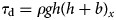 and $\tau _{\rm b}$
 defined by (4), for $C = 1.5\times$
 10$^7$
 Pa m$^{-1/3}$
 s$^{1/3}$
 ; (b) $\tau _x$
 (kPa). The simulation parameters are the following: bed elevation $\displaystyle {b( x) = b_0 + b_{\rm a} {\rm cos} {\pi x\over L}}$
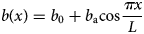 , with $b_0 = -500$
 m, $b_{\rm a} = 250$
 , and $L = 500$
 km; accumulation rate $\dot a = 0.6$
 m a$^{-1}$
 ice stiffness parameter $A = 1.35\times$
 10$^{-25}$
 Pa$^{-3}$
 s$^{-1}$
 (corresponds to $T_{{\rm ice}}\approx$
 -20$^\circ$
 C). In all simulations the ice flow is from left to right.
Fig. 9. Effects of the buoyancy parameter $\delta$ , the flow-law exponent $n$
 and the sliding-law exponent $m$
 on the momentum balance (a–b) $\delta = 0.1$
 , $n = 3{1\over 3}$
 , $m = {1\over 3}$
 ; (c) $\delta = 0.1$
 , $n = m = 1$
 ; (d) $\delta = 0.9$
 , $n = m = 1$
 . The simulation parameters are the following: bed elevation $\displaystyle {b( x) = b_0 + b_{\rm a} {\rm cos} {\pi x\over L}}$
 , with $b_0 = -500$
 m, $b_{\rm a} = 250$
 , and $L = 500$
 km; (a–b) $C = 1.5\times$
 10$^7$
 Pa m$^{-1/3}$
 s$^{1/3}$
 , $A = 1.35\times$
 10$^{-25}$
 Pa$^{-3}$
 s$^{-1}$
 , $\dot a$
 = 0.1 m a$^{-1}$
 ; (c) $C = 1.5\times$
 10$^{10}$
 Pa m$^{-1}$
 s$^{1}$
 , $A = 5.13\times$
 10$^{-15}$
 Pa$^{-1}$
 s$^{-1}$
 , $\dot a = 0.7$
 m a$^{-1}$
 ; (d) $C = 3.8\times$
 10$^{10}$
 Pa m$^{-1}$
 s$^{1}$
 , $A = 5.13\times$
 10$^{-15}$
 Pa$^{-1}$
 s$^{-1}$
 , $\dot a = 510$
 m a$^{-1}$
 , $\delta = 0.9$
 . In all simulations ice flow is from left to right.
There are, then, two effects that contribute to the weakness of the boundary layer. The first is the smallness of $\delta$ , and that the more similar $\delta$
 becomes to $\varepsilon$
 the weaker the boundary layer becomes. However, the non-linearity of the flow and the basal friction are also important contributors. One might suppose that a more distinct boundary layer behaviour will emerge as $\phi$
 becomes larger and $\delta$
 closer to 1. This is illustrated in Figures 9c and 9d, which show an example in which $\varepsilon = 6.4\times 10^{-4}$
 . Linearising the flow and the basal friction by setting $n = m$
 = 1, $\phi$
 takes the value of 3, and in this case (Fig. 9c) a distinct boundary layer is visible in the longitudinal stress gradient. If we also allow $\delta$
 to be close to 1, the boundary layer becomes pronounced (Fig. 9d) just as one would suppose.
Appendix B. Stability analysis
Here we describe a linearised stability analysis of the steady-state problem. Considering small perturbations (of the order of a small parameter $\sigma$ ) around the steady state,

where we denote steady states by a symbol $\hat{}$ , and substituting these expressions into (14) leads to the perturbation problem to the lowest order in $\sigma$


and


Substituting this expression into (B2b) leads to a parabolic partial differential equation (PDE) for $\tilde H$

Using the method of separation of variables one arrives at the form

Substituting $\tilde H$ in this form into (B4) and writing (B2b) as $\tilde Q_X = -\Lambda \tilde H$
 gives
gives


and

where


and

which is a second-order eigenvalue problem with $\Lambda$ being the eigenvalue. It is not possible to obtain a closed form expression for the values of $\Lambda$
 . However, the stability depends only on the sign of $\Lambda$
 .
.
If all $\Lambda \lt$ 0, then small perturbations $\tilde H$
 and $\tilde Q$
 decay with time, and such a steady-state ice-sheet configuration is stable; on the other hand, if at least one eigenvalue $\Lambda \gt$
 0, then small perturbations grow with time and such a steady-state ice-sheet configuration is unstable.
To determine the sign of eigenvalues we follow Schoof (Reference Schoof2012) in putting (B6a) into a Sturm–Liouville form,

using the integrating factor

where


and

If one substitutes (B9) and (B10) into (B8) one can, with a little algebra, recover (B6a) and so show that (B6a) can be put in a Sturm–Louville form. The functions $\mu$ , $P$
, $P$ and $R$
 are continuous, $\mu ( X) P( X)$
 is a positive function, and the boundary conditions (B6b) and (B6c) can be written as homogeneous functions of $\tilde H$
 and $\tilde H_X$
 .
.
However, in contrast to a Sturm–Lioville problem considered by Schoof (Reference Schoof2012), the problem (B6) is not a regular Sturm–Liouville problem, due to the presence of the eigenvalue $\Lambda$ in the boundary condition (B6c). There is a body of literature devoted to Sturm–Liouville problems in which the eigenvalue appears in the boundary conditions (e.g. Amrein and others, Reference Amrein, Hinz and Pearson2005). In particular, one can show using theorem 1 of Linden (Reference Linden1991) that for the Sturm–Lioville problem (B8) with boundary conditions (B6b) and (B6c), the $k$
 th eigenfunction has $k-1$
 zeros, and consequently, the eigenfunction corresponding to the largest eigenvalue does not have zero crossings, provided that in addition to the continuity, positivity and homogeneity conditions of the regular problem, the inequality

is satisfied. With the use of the steady-state momentum balance (14a) this condition reduces to


Substituting (B13) into (B6c) and using the relations $\hat Q_{X} = \dot a$ and (B2a), one may arrive at:

The sign of $\Lambda$ in the above expression is determined by the steady-state properties at the steady-state grounding-line position, except the term ${( {\int _0^{\hat X_{\rm {g}}}\tilde H{\rm d}x}) /{\tilde H}}$
 that appears in the first square-bracketed term on the right-hand side of (B14). As we have noted, the largest eigenvalue (that corresponds to the fastest growing or slowest decaying perturbations of the steady states) is associated with eigenfunction with no zeros. In consequence, for these eigenvalues, the term $( {{\int _0^{\hat X_{g}}\tilde H{\rm d}x}) /{\tilde H}}$
 is positive. This does not of itself suffice to determine the sign of the largest eigenvalues. However, one can show using the steady-state momentum balance (14a) that with (B12) satisfied, the first square-bracketed term on the right-hand side of (B14) is positive for this maximum eigenvalue; and if

the second square-bracketed term is negative. As Schoof (Reference Schoof2012) observes, (B15) must be satisfied if the steady solution is to remain grounded upstream of the grounding line, and it may be regarded as satisfied for any steady solution to the problem. With $m > 0$ , $\delta < 1$
 and $B_X > 0$
 , (B12) is satisfied if (B15) is satisfied, and in this case, the stability can be determined from the sign of the third square-bracketed term of (B14): if

the grounding line is stable. However, if $B_X < 0$ , it is (B15) that is satisfied if (B12) is satisfied, and it is then (B12) that must be satisfied for stability to be determined by (B16).
To validate the above results, we solve (B6) numerically with the finite-element solve ComsolTM (COMSOL, 2021). We compute eigenvalues and eigenfunctions for the steady-state ice-sheet configurations for the smooth and undulating bed topographies. Figures 10 and 11 show examples of the ten largest eigenvalues and first four eigenfunctions for stable and unstable grounding-line positions. For all stable positions, all the eigenvalues are negative (Figs 10b and 11b); for all unstable positions, the largest eigenvalue is positive, and all others are negative (Figs 10d and 11d). The eigenfunctions corresponding to the largest eigenvalues for both stable and unstable steady-state configurations do not have zeros, consistent with the theorem of Linden (Reference Linden1991).

Fig. 10. Eigenvalues and eigen-functions for the long-wavelength bed topography. (a) Stable (open circle) and unstable (crossed circle) steady-state grounding line positions; (b) first ten eigenvalues $\Lambda$ (s$^{-1}$
 ) for the stable position (open circle); (c) first four eigen-functions $\tilde H$
 (m) for the stable position (open circle); (d) first ten eigenvalues $\Lambda$
 (s$^{-1}$
 ) for the unstable position (crossed circle); (e) first four eigen-functions $\tilde H$
 (m) for the unstable position (crossed circle).
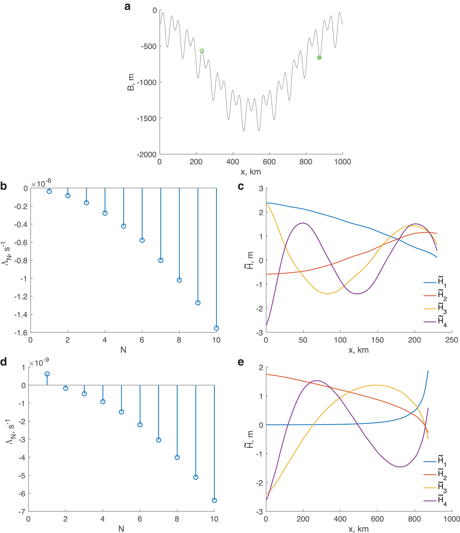
Appendix C. The longitudinal stress gradient at the grounding line
Equations (18) and (19) assume that the longitudinal stress gradient in the momentum equation is negligible. For the case in which the basal gradient is dropped from the momentum equation, we examined in Appendix A the error that results from ignoring the longitudinal stress gradient by substituting the solutions of the reduced equation (A6) back into the full equation (A2a). When the basal gradient can not be ignored, the corresponding equations are (14a) and (13a) but for these we do not have solutions. However, even without the solutions, we can estimate the longitudinal stress gradient at $X_{\rm {g}}$ , which is what we do in this appendix. Specifically, we write the longitudinal stress gradient in the form

and use the reduced Eqns (14a) to estimate the terms in (C1), from which we can determine the circumstances in which it may be regarded as a small.
To compute various terms of this expression we use (14), that yields


and

Differentiating (C2b) to obtain an expression for $U_{XX}$ and eliminating from it $H_{XX}$
 through differentiating (C2a) one can obtain with a second use of (C2a)

Eliminating $Q$ from (18) using $Q = UH$
 one can with (C2c) obtain an expression for ${{U^{m + 1}}/{H^3}}$
 which, when substituted into the RHS of (C3) provides

Substituting (C4) into the RHS of (C1)

Using (C2a) and (C2c) and eliminating $U$ using ${U = {Q}/{H}}$
 provides, finally

With $\delta$ = 0.1 and $n = {1\over m}$
 = 3, the leading coefficient of the first term on the right is 0.006; the leading coefficient of the second term is zero; and with $\varepsilon$
 = 0.07, the largest value of those in Fig. 5, the leading coefficient of the third term is 0.05. Thus, we expect in these circumstances that the dropping of the longitudinal stress gradient in forming (18) and its dimensional form (25) will remain a good approximation.


 Open access