


Introduction
Glacier loss affects freshwater availability, particularly on seasonal timescales in mountain catchments (Fountain and Tangborn, Reference Fountain and Tangborn1985; Moore and others, Reference Moore2009). Runoff from alpine glaciers not only acts as a buffer against low flows and warm stream temperatures (Brown and others, Reference Brown, Hannah and Milner2005; Moore, Reference Moore2006), but also provides fluxes of nutrients important to aquatic ecosystems (Hood and Berner, Reference Hood and Berner2009; Milner and others, Reference Milner2017). Estimates of initial glacier volume are required to simulate future glacier mass loss and contribution to streamflow on regional and global scales (Hock and others, Reference Hock2019). Methods to estimate regional or global glacier volume typically employ an inverse model using volume-area scaling relations (e.g. Radić and Hock, Reference Radić and Hock2010), neural networks (e.g. Clarke and others, Reference Clarke, Berthier, Schoof and Jarosch2009) or mass conservation schemes (e.g. Farinotti and others, Reference Farinotti, Huss, Bauder, Funk and Truffer2009; Morlighem and others, Reference Morlighem2011; Paul and Linsbauer, Reference Paul and Linsbauer2012). Farinotti and others (Reference Farinotti2017) intercompared a large suite of these methods, and showed that physically-based models perform better than volume-area scaling, but the models produce a very large spread in predicted ice thickness. The performance of these models suffers from the lack of observational data the models need as an input or boundary conditions (e.g. observations of mass balance and surface velocity). Measurements of ice thickness are only available for about 5000 of Earth's > 200 000 glaciers (GlaThiDa, 2019). The lack of data with which to assess model predictions makes reducing the large spread of model predictions challenging.
Ice thickness data in Western North America-WNA, region 02 of the Randolph Glacier Inventory (RGI) V6 (Pfeffer and others, Reference Pfeffer2014), are equally sparse, with mean ice thickness reported for 36 glaciers; 34 of which are within the contiguous United States, a region containing less than 4% of ice area in WNA. In western Canada, south of Yukon, glacier thickness measurements are presently available for only West Washmawapta Glacier, a small (0.9 km2) cirque glacier (Sanders and others, Reference Sanders, Cuffey, MacGregor, Kavanaugh and Dow2010), the toe of the Athabasca Glacier (Ommanney, Reference Ommanney2002) and the toe of the Peyto Glacier (Kehrl and others, Reference Kehrl, Hawley, Osterberg, Winski and Lee2014). Additional thickness measurements were acquired at Peyto Glacier in 1983–1985 (Holdsworth and others, Reference Holdsworth, Demuth, Beck, Demuth, Munro and Young2006), but the glacier has undergone significant thinning since (Demuth and Keller, Reference Demuth and Keller2006; Kehrl and others, Reference Kehrl, Hawley, Osterberg, Winski and Lee2014).
Western Canadian ice volume was estimated by several previous studies (Huss and Farinotti, Reference Huss and Farinotti2012; Clarke and others, Reference Clarke2013; Farinotti and others, Reference Farinotti2019) which primarily use surface inversion. Mass-conservation models either parameterize or simulate a surface mass-balance gradient, then utilize topographical information from digital elevation models (DEMs) to estimate the distribution of the glacier's surface mass balance and thus its mass turnover. Alternatively, models may ingest fields of surface mass balance (Brinkerhoff and others, Reference Brinkerhoff, Aschwanden and Truffer2016). Mass turnover is then inverted for ice thickness using a model of ice flow. Clarke and others (Reference Clarke2013) provided the first distributed estimate of ice volume for all glaciers in western Canada that lie south of 60°N. Their model calculates ice flux through flux gates by integrating the apparent mass balance (mass balance – height change (δh/δt)) over the upstream area associated with each gate. Despite successful overall performance, the agreement between their modeled and measured ice thickness at three surveyed glaciers in western Canada could not be achieved without additional corrections to the assumed bed stress and thinning rates.
The goal of our study is to complement and advance the current ice thickness database for Canadian glaciers. We do so by (1) incorporating new measurements of ice thickness obtained by ice penetrating radar from glaciers in the Columbia River basin, and (2) comparing the measured to modeled ice thickness of these glaciers with the use of an inverse model developed by Maussion and others (Reference Maussion2019). As a final objective, we use the inverse model to assess the ice thickness over a full suite of glaciers in the Canadian portion of the Columbia River basin and to quantify the region's total ice volume.
Study area
The 2000 km-long Columbia River is the fourth largest river in North America by discharge and is one of the most heavily developed transboundary water resources in North America (Cohen and others, Reference Cohen, Miller, Hamlet and Avis2000). The Columbia River basin covers nearly 670 000 km2 and encompasses portions of seven states of the United States and the Canadian province of British Columbia (BC) (Fig. 1). The basin produces over 40% of hydroelectricity in the United States (U.S. Energy Information Administration, 2018), more than any other river system in North America. The Canadian portion of the upper Columbia Basin, hereafter referred to as ‘the Basin’, represents 15% of the watershed's total area (Fig. 1) yet provides 30–40% of its total runoff, predominately from snowmelt (Cohen and others, Reference Cohen, Miller, Hamlet and Avis2000). For the specific names of the glacierized watersheds within the Basin and the glacierized mountain ranges within the Columbia and Canadian Rocky mountains refer to Troffe (Reference Troffe1999) and Ommanney (Reference Ommanney2002), respectively. There are around 2100 glaciers covering 1750 km2 in the Basin, with a variety of glacier types including icefields, valley glaciers and cirque glaciers (Ommanney, Reference Ommanney2002). Five of our seven study glaciers (Table 1) lie within the Columbia Mountains while West Washmawapta and Haig glaciers lie within the Rocky Mountains (Fig. 1). Glaciers contribute 20–35% of late-summer flow and about 6% annually to the Basin headwaters above Mica Dam (Jiskoot and Mueller, Reference Jiskoot and Mueller2012; Jost and others, Reference Jost, Moore, Menounos and Wheate2012). Glacier loss in the Canadian Rocky Mountains region of the study area was around 30% between 1919 and 2006 and has been accelerating since the 1980s (Jiskoot and others, Reference Jiskoot, Curran, Tessler and Shenton2009; Tennant and others, Reference Tennant, Menounos, Wheate and Clague2012). Most of the glaciers are projected to disappear by 2100, with peak glacial runoff to occur around 2020–2040 (Clarke and others, Reference Clarke, Jarosch, Anslow, Radić and Menounos2015). The majority of glaciers in the Basin are too small to have been included in the first regional baseline ice flow maps (Van Wychen and others, Reference Van Wychen2018) and velocity estimates (Gardner and others, Reference Gardner, Fahnnestock and Scambos2019).
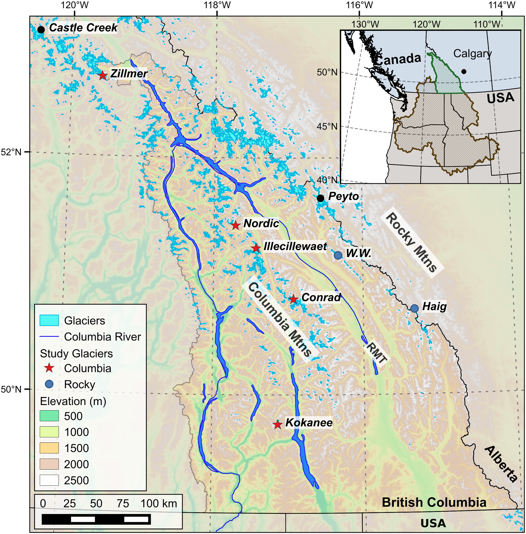
Fig. 1. Columbia River Basin and study glaciers map. Inset shows the Canadian portion (green) of the Columbia River basin (brown) which contributes to the river where it crosses the international border. Map coordinates are in WGS84/UTM11.
Table 1. Characteristics of study glaciers

Glacier area is RGI version 6.0 area except for Nordic and Illecillewaet glaciers, which were calculated with corrected outlines.
Data and methods
Ice thickness measurements
To measure ice thickness for the glaciers in the Basin, we conducted ice-penetrating radar (IPR) surveys in April–May of 2015–2018. We used a Blue System Integration radar system, employing 10 MHz center frequency antennas (Mingo and Flowers, Reference Mingo and Flowers2010) and a ± 550 volt impulse transmitter (Narod and Clarke, Reference Narod and Clarke1994) paired with resistively-loaded transmitting and receiving dipole antennas arranged parallel to the direction of survey with 15 m separation. Record length was typically 300–1200 with a transmitter pulse repetition frequency of 512 Hz. Triggering for the digitizer was initiated by the air-wave arrival and generally 25–256 waveforms were stacked per recorded trace. This resulted in a recorded wave for each 3–5 m of surface travel. We collected radar data along longitudinal and cross-profiles, but followed safe travel routes.
A Garmin NMEA GPS18x Global Positioning System (GPS) receiver with an estimated positional accuracy of ± 3 m recorded coordinates of each radar sounding. In total, we collected 190 line km of data (Table 2) across five glaciers. Bedrock reflections exist for 169 of the 190 line km of data (31 703 point measurements of ice thickness, Fig. 2). Surveys of Haig (Adhikari and Marshall, Reference Adhikari and Marshall2011) and West Washmawapta (Sanders and others, Reference Sanders, Cuffey, MacGregor, Kavanaugh and Dow2010) glaciers included an additional 13 km of traverses and 2969 measurements of ice thickness.

Fig. 2. Ice thickness measurements (Table 2) for (a) Kokanee, (b) Haig, (c) Conrad, (d) West Washmawapta, (e) Illecillewaet, (f) Nordic and (g) Zillmer glaciers. Coordinates are °N and °W. Scale differs among glaciers. Figures S1–S7 contain detailed maps with LiDAR DEM hillshades.
Table 2. Ice thickness survey year, total distance surveyed, total distance used (with a bed picked), total number of measurements of the bed (n), glacier surface area coverage, 100 m elevation bin coverage and hypsometric coverage

Coverage was assessed on a 200 m grid.
Radar processing
We extracted ice thickness using Radar Tools, part of the open-source irlib Python package (Wilson, Reference Wilson2017), and assumed a radar wave propagation velocity of 168 m μs−1 (e.g. Glen and Paren, Reference Glen and Paren1975) and a parallel-planar geometry of the surface and base near the measurements (Adhikari and Marshall, Reference Adhikari and Marshall2013). Signal filtering allowed us to better distinguish bed versus englacial reflections. For all data, we applied a high-pass (dewow) filter, time-proportional gain control of varying magnitude and a low-pass filter (Fig. 3). Low-pass filtering reduced noise and high-frequency clutter while enhancing the bed reflection. The amount of low-pass filtering required varied among lines, particularly in the accumulation areas, where noise and clutter were prevalent. After filtering, we picked radar traces using icepick2 (Wilson, Reference Wilson2017).
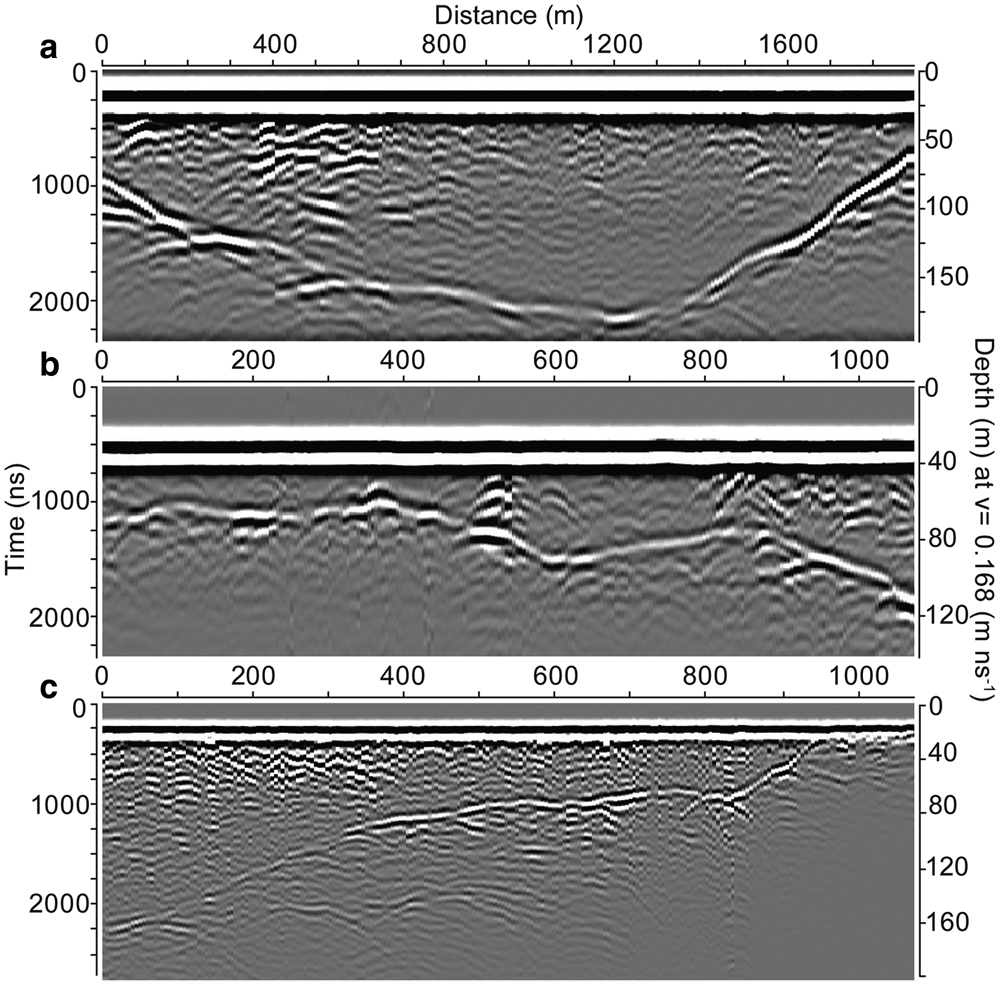
Fig. 3. Radargrams from (a) Conrad, (b) Nordic and (c) Illecillewaet glaciers. Each radargram has been highpass (dewow) and lowpass filtered.
Ice thickness modeling
To simulate ice thickness, we used a model developed by Maussion and others (Reference Maussion2019), hereafter referred to as Open Global Glacier Model (OGGM v1.3.1, Maussion and others, Reference Maussion2020). We chose OGGM because: (1) it performed well for alpine glaciers in a model intercomparison study (Farinotti and others, Reference Farinotti2017), among the models with few data requirements; (2) is open-source; and (3) can be applied to all glaciers globally. OGGM is a depth-integrated flowline model where ice thickness is computed via mass-conservation with estimates of ice velocity and ice flux obtained from the physics of ice flow and mass balance. The model is solved along multiple flowlines computed with the algorithm of Kienholz and others (Reference Kienholz, Rich, Arendt and Hock2014). Depth-integrated ice velocity is computed using the shallow ice approximation. The mass-balance model implemented in OGGM builds on the temperature index model presented by Marzeion and others (Reference Marzeion, Jarosch and Hofer2012). The mass-balance model ingests climate data and relies on a temperature sensitivity parameter (Marzeion and others, Reference Marzeion, Cogley, Richter and Parkes2014, Reference Marzeion, Jarosch and Hofer2012) which is calibrated using glaciers with observations of specific mass balance available from Fluctuations of Glaciers (FoG) Database (WGMS, 2018). Instead of running the mass-balance model, we used our observed mass-balance gradients to prescribe mass balance. When running OGGM without our in situ balance gradients, we ingest Climatic Research Unit Timeseries v.4.01 temperature and precipitation data downscaled with an anomaly mapping approach (Harris and others, Reference Harris, Jones, Osborn and Lister2014). Rather than parameterize apparent mass balance, OGGM assumes steady-state (δh/δt = 0) so the mass balance equals the apparent balance. We used a lower-slope limit of 1.5° to prevent an overestimation of ice thickness in flat zones. Detailed description and documentation of the model can be found in Maussion and others (Reference Maussion2019) and online (http://oggm.org).
We set sliding velocity to zero in this study due to the spatial complexity of sliding that we suspect for our glaciers. Negligible sliding was observed for Haig (Adhikari and Marshall, Reference Adhikari and Marshall2013) and West Washmawapta glaciers (Sanders and others, Reference Sanders, Cuffey, MacGregor, Kavanaugh and Dow2010). By neglecting sliding velocity, all uncertainties regarding sliding are transferred to the creep (A) parameter from Glen's flow law (Glen, Reference Glen1955). The larger A is, the less rigid the ice is, which drives increased flux and thus a thinner glacier.
To compare our point observations to gridded ice thickness model output, we aggregated our observations to a grid with position and resolution matching the model output. This aggregation prevents grid cells with greater number of observations from being more heavily weighted than grid cells with fewer observations. We chose not to interpolate our observations to avoid creating pseudo-data to compare against the model.
Our methodology, regarding the model setup and runs, can be split into the following steps: (1) data preprocessing to prepare the input to OGGM, (2) model calibration and cross-validation, and (3) application of the model for the Basin ice volume assessment. In the following sections we present each of these steps in more detail.
Preprocessing of input data
OGGM requires the following input data provided by the user: glacier surface topography, glacier outlines and surface mass-balance gradients. For a consistent comparison between the modeled and measured ice thickness at our glaciers, we used a LiDAR DEM acquired during the year of our ice thickness measurements (Pelto and others, Reference Pelto, Menounos and Marshall2019) for surface inversion. OGGM and the three published estimates of ice thickness (Huss and Farinotti, Reference Huss and Farinotti2012; Clarke and others, Reference Clarke2013; Farinotti and others, Reference Farinotti2019) utilized the Shuttle Radar Topographic Mission (SRTM) DEM (Jarvis and others, Reference Jarvis, Reuter, Nelson and Guevara2007). To quantify the elevation difference between a given LiDAR DEM used for surface inversion and the SRTM used for previous estimates of ice thickness, we coregistered our LiDAR DEMs and the SRTM DEM following the procedure of Nuth and Kääb (Reference Nuth and Kääb2011) and then calculated the difference (ΔDEM) between these coregistered DEMs (Fig. 4). For Haig Glacier, we calculated an annual elevation change rate from the ΔDEM and multiply by the number of years between the May 2009 radar survey and SRTM acquisition (Table 3). We lack a LiDAR DEM for West Washmawapta Glacier, so we multiplied the annual elevation change rate of Haig Glacier, also located in the Rocky Mountains (Fig. 1), by the number of years between SRTM and the 2006 ice thickness observations (Sanders and others, Reference Sanders, Cuffey, MacGregor, Kavanaugh and Dow2010). The SRTM DEM, acquired in C-band (~5.6 cm), underestimates glacier elevations since the radar signal at this wavelength is typically estimated to average 1–4 m penetration on temperate glaciers (Rignot and others, Reference Rignot, Echelmeyer and Krabill2001; Gardelle and others, Reference Gardelle, Berthier, Arnaud and Kaab2013). Since this penetration is difficult to correct for we did not bias correct ΔDEM estimates (Table 3).

Fig. 4. Conrad Glacier SRTM–LiDAR height change. LiDAR DEM is from 12 September 2016.
Table 3. Total SRTM–LiDAR height change on-ice and off-ice with 2-σ height change uncertainty assessed over stable terrain after correction for effective sample size as detailed in Pelto and others (Reference Pelto, Menounos and Marshall2019)

aWest Washmawapta Glacier height change is estimated using the annual rate of Haig Glacier height change and does not contribute to averages.
To represent our glaciers within OGGM, we extracted glacier outlines from RGI V6 (Pfeffer and others, Reference Pfeffer2014) which date to 2005 in the Basin (Bolch and others, Reference Bolch, Menounos and Wheate2010). Nordic and Illecillewaet glaciers are improperly represented in RGI, so we corrected their outlines (Fig. S8). The ice divide of Illecillewaet Glacier is mismapped, omitting a section of its accumulation zone. A mis-classified medial moraine (Fig. S9) and attached but separate branch were corrected for Nordic Glacier (Fig. S8) as described elsewhere (Supplemental S2).
We used surface mass-balance observations to define balance gradients in OGGM (Table 4) for all study glaciers. We approximated the balance gradient of West Washmawapta Glacier as the average of the balance gradients of Peyto (6.14 mm w.e. m−1) and Haig glaciers (Young, Reference Young1981; Marshall and others, Reference Marshall2011). West Washmawapta Glacier is located 50 km south of Peyto Glacier, and 90 km northwest of Haig Glacier (Fig. 1). The annual balance of the Columbia Mountain glaciers typically ranges from +1 to +2.5 m water equivalent (w.e.) in the accumulation area to − 4 to − 7 m w.e. near the terminus (Pelto and others, Reference Pelto, Menounos and Marshall2019).
Table 4. Modeled and observed balance gradients in mm w.e. m−1

Number of observations (n).
Model calibration and cross-validation
To produce a best estimate of mean ice thickness and total ice volume for each glacier, we applied our in situ balance gradients and minimized mean absolute error (MAE) between observed and modeled ice thickness for every glacier by tuning the A parameter within the shallow-ice approximation:

where n is the number grid cells where both gridded observations of ice thickness (H obs) and those estimated by OGGM (H mod) exist. We chose to tune A because currently A is the only free parameter within OGGM. The optimal A (A opt) is the one that produces the minimum MAE (MAEmin) according to the k-folding cross-validation explained below. Our model set-up is also aimed at reproducing average glacier thickness for calculating total ice volume. Like for MAE, we evaluate mean error (ME) between all observed and modeled ice thickness, but do not use ME within the optimization.
Similar to Helfricht and others (Reference Helfricht, Huss, Fischer and Otto2019), we applied cross-validation for estimating the model performance in reproducing both single ice thickness measurements at the individual glaciers and average ice thickness. Ice thickness measurements (Table 1) were aggregated to the model grid of each study glacier. To minimize the effect of spatial autocorrelation and better quantify out-of-set predictive error, we followed the procedure described by Pelto and others (Reference Pelto, Menounos and Marshall2019) to estimate decorrelation length of our gridded ice thickness observations. We found decorrelation lengths from 250 to 1100 m, with an average of 500 m. Based on these distances, we grouped gridded observations at the transect level so that the distance between them exceeds the decorrelation length for a given glacier. These groupings ranged from six groups for West Washmawapta Glacier to 19 groups for Conrad Glacier, and averaged ten groups. We then applied a twofold cross-validation to assess model uncertainty: (1) grouped observation data were split into two subsets, with 80% as a training dataset and 20% as a test dataset; (2) by randomly pulling the data points from the training dataset, the dataset was further split into two equal subsets (50% each, still grouped) representing calibration and validation data; (3) the model was then run on the calibration dataset for a set of A values; (4) A associated with MAEmin over the calibration data was then used to run the model over the validation data; (5) steps 3 and 4 were repeated 50 times with the calibration-validation dataset split each time; (6) the A associated with the smallest MAEmin from the 50 runs over the validation data was taken as A opt; and (7) the A opt was used to run the forward model to produce the best estimate of ice thickness and ice volume (V) for a given glacier. To estimate the model error, the forward model with A opt was run over the test data, held out in step 1.
Model application for the Basin
To estimate ice volume of the Basin, we derived a single mass-balance gradient and an A parameter for the Basin. We took the average of the balance gradients from eight glaciers (7.74 ± 1.6 mm w.e. m−1), five within the Basin and three glaciers proximal to the Basin: Peyto, Haig and Castle Creek glaciers (Table 4). Beedle and others (Reference Beedle, Menounos and Wheate2014) published Castle Creek Glacier mass-balance data from 2008 to 2013 which we supplement with new measurements from 2014 to 2019. Castle Creek Glacier is located 55 km NW of the Basin and 67 km NW of Zillmer Glacier (Fig. 1). The Basin A was determined by calibrating ice thickness for all seven glaciers simultaneously while minimizing MAE. Gridded observations were corrected by gridded SRTM–LiDAR height change to represent glacier ice at the time of SRTM acquisition. The Basin balance gradient and A were then used for the model run for each individual glacier in the Basin with the glacier outlines provided in RGI V6. For each glacier we estimate its mean thickness $\bar {H}$ . Multiplying $\bar {H}$
 with the glacier's surface area S we derive its volume. Total ice volume of the Basin is the sum of V for all (N) glaciers in the region.
Error in glacier area (σS) each individual glacier was calculated using the buffering method proposed in Granshaw and Fountain (Reference Granshaw and Fountain2006):

where i is the i-th glacier in the Basin, the buffer is the resolution of a pixel, dx, and P denotes the length of the perimeter of the glacier. We set dx=30 m since glacier outlines in our region were predominately derived from 30 m imagery (Bolch and others, Reference Bolch, Menounos and Wheate2010). The average relative error (RE), derived as the mean RE of the seven glaciers (0.08, where ${\rm RE} = {\rm ME}/\bar {H}$ ), was used to calculate ice thickness error for each individual glacier in the Basin as: $\sigma _{{\rm H}\comma i} = {\rm RE}_i \cdot \bar {H_i}$
 . A random error (V rand) in the estimate of Basin ice volume is calculated by propagating σS and σH for each glacier (i) in the Basin, and summing these errors:

Uncertainty on the SRTM–LiDAR height change correction (σδh,SRTM), which we used to adjust observations to the SRTM acquisition date, was taken as 1.6 m, the 2-σ height change uncertainty (Table 3). This error was then assessed for the Basin ($\sigma _{{\rm V}_{\rm SRTM}}$ ):
):

Systematic error (V sys) was assessed by quantifying the effect of possible A values on Basin ice volume. The range of A was determined using a leave-one-out (Molinaro and others, Reference Molinaro, Simon and Pfeiffer2005) optimization where one of our seven glaciers was randomly withheld while optimizing A to minimize MAE over ten simulations. We then estimate the upper and lower bound for Basin ice volume using the minimum and maximum A value from the range of optimized leave-one-out A values. The systematic error is then assumed to be the larger of the two differences: |V upper − V ref| and |V lower − V ref|. We then combine random, SRTM and systematic error to estimate total Basin ice volume uncertainty:

Results
Our average observed ice thickness across the seven glaciers was 92.5 m with average, gridded observations that range from 47.7 to 138.6 m (Table 5). Maximum ice depth was observed at Conrad Glacier (318 m). Measurement coverage, as assessed on a 200 m grid, averaged 73% but was below 50% for Zillmer Glacier (Table 2). Average coverage of 100 m elevation bins was 89% but hypsometric coverage, or the glacier area represented by the elevation range covered, averaged 96% (Table 2). Gridding the ice thickness observations to 200 m resolution did not change the mean ice thickness by more than 2% for any glacier except Haig Glacier (Table 5).
Table 5. Optimized model run outputs and observed ice thickness

Model runs used in situ balance gradients and were optimized by tuning Glen's A to minimize MAE between observed and modeled ice thickness. Flowline thickness represents average ice thickness along the primary glacier flowline.
Modeled ice thickness with optimized A values for each glacier yields an average ice thickness of 72 m and ranges between 40–99 m (Table 5). Optimized ice thickness for each glacier (Fig. 5) had an average model bias of –3.8 ± 3.7% (Table 6). Average A opt for all glaciers was 6.37 × 10⁻²⁴ Pa−3 s−1 (Table 5). Average ME decreased twofold from the default-settings OGGM run relative to the optimized run (Table 6). MAE decreased by 7.6% from 32.0 m with the default runs to 22.1 m when optimized. Optimization produced lower per cent error for smaller glaciers with relatively simple geometries such as Haig, Kokanee and West Washmawapta relative to the larger, more complex glaciers. The greatest discrepancies between measured and OGGM-derived ice thickness occur over gentle terrain (Fig. 6). The largest deviation was near the center of Conrad Glacier (Fig. 6). IPR observations of ice thickness are less than calibrated OGGM ice thickness over the tongue (< 2400 m) of Conrad Glacier by 9.9%. Correlation between slope and the model bias was weak but statistically significant: r = −0.29 (p − value < 0.01, n = 3703) for MAE, and r = −0.09 (p − value < 0.01) for ME. Ice flux and MAE had a weak correlation (r = 0.25, p − value < 0.01).

Fig. 5. Optimized ice thickness for (a) Kokanee, (b) Haig, (c) Conrad, (d) West Washmawapta, (e) Illecillewaet, (f) Nordic and (g) Zillmer glaciers.

Fig. 6. Difference between radar observations of ice thickness and optimized OGGM modeled ice thickness for (a) Kokanee, (b) Haig, (c) Conrad, (d) West Washmawapta, (e) Illecillewaet, (f) Nordic and (g) Zillmer glaciers. Note scale differs between glaciers. Coordinates are °N and °W. Positive values are greater observed ice thickness relative to modeled.
Table 6. Mean absolute error (MAE) and mean error (ME) between observed and modeled ice thickness for all seven glaciers for the individual optimized ice thicknesses, default OGGM run and optimized Basin ice volume run

MAE is minimized by tuning A during model calibration.
Observed mass-balance gradients are larger than those modeled by OGGM (Table 4 and Fig. 7). While we used observed mass-balance gradients within the optimized OGGM run for each study glacier, the average deviation between observed and modeled mass-balance gradients was –4.18 ± 2.1 mm w.e. m−1 or about $-70.5\percnt$ (Table 4). Using the observed instead of modeled balance gradients produced, on average, 15.6% thicker ice (Fig. 8) and improved, on average, estimated ice thickness by 4.4%. Model runs with observed balance gradients yielded smaller bias for three glaciers (Haig, Nordic and West Washmawapta), but produced larger errors for the remaining glaciers (Table 4, Fig. 8). Using the updated glacier outlines instead of those from RGI V6 for Illecillewaet and Nordic glaciers slightly increased the balance gradients (by 3–6%) and the ice thickness (by 13%), while reducing the model bias (Fig. S8).

Fig. 7. Observed balance gradients versus OGGM-derived mass-balance gradients for (a) Kokanee, (b) Haig, (c) Conrad, (d) West Washmawapta, (e) Illecillewaet, (f) Nordic and (g) Zillmer glaciers.

Fig. 8. Comparison of ice thickness for the seven study glaciers: (a) modeled ice thickness with OGGM-derived mass-balance gradients versus modeled ice thickness with observed gradients; (b) modeled ice thickness with OGGM-derived and observed mass-balance gradients versus observed ice thickness. The arrows point from modeled ice thickness using an OGGM-derived mass-balance gradient to modeled ice thickness using an observed mass-balance gradient. Dashed lines are one-to-one lines.
Using the SRTM DEM for the inversion produced 2.3% greater ice thickness relative to the LiDAR DEMs despite an average thinning of 6% over this period. Using LiDAR DEMs instead of the SRTM DEM reduced model bias for specific locations (e.g. steep slopes) but only by <5% on average. We found an average height change of − 5.43 ± 1.6 m of between the SRTM and LiDAR DEMs (Table 3), for an average rate of − 0.32 ± 0.11 m a−1. Average SRTM–LiDAR height change off-glacier was − 0.12 ± 0.5 m (Table 3), with large differences existing only over steep terrain, suggesting comparisons over the glaciers are reliable. Over the accumulation areas, we observed slight thickening in general + 2.5 ± 2.7 m (Fig. 4), despite previous findings that accumulation areas have thinned over this period (Pelto and others, Reference Pelto, Menounos and Marshall2019). This apparent thickening is likely due to SRTM radar signal penetration into firn.
We did not find a consistent trend in ice thickness with varying spatial resolution of input topography. A difference of $-1 \pm 8\percnt$ in ice thickness existed between ice thickness estimates produced from DEMs of 10 and 30 m (range: − 12 to +7%). Using a 90 m DEM produces ice that was $4.5\pm 12\percnt$
 thicker (range: − 12 to +21%) than with a 30 m DEM. Spatial resolution of the DEM affects steepest ice most (e.g. Nordic and Kokanee glaciers), but the use of 100–200 m resolution DEMs produces ice volume within 3% of that estimated from higher-resolution DEMs. While DEM resolution affects the distance over which slope is calculated, we found that model bias in at-a-point ice thickness was only weakly correlated with estimated surface slope and modeled ice flux across all the points. We also found no statistically significant correlation between relative model error and DEM resolution across our study glaciers.
Our simultaneous optimization of A across the seven study glaciers produced a A opt of 4.82 × 10⁻²⁴ Pa−3 s−1. Finally, using our Basin balance gradient of 7.74 mm w.e. m−1 and Basin A opt, we estimated total ice volume (V ± σV) of 122.5 ± 22.4 km3 for the Basin. This volume is based on the SRTM surface, thus represents glacier volume as of year 2000. For our study glaciers, MAE and ME are lower with the Basin run settings than with default OGGM settings (Table 6). With the leave-one-out approach to assess systematic uncertainty, we find that the A values thus yield a range of Basin ice volumes from 9% smaller to 15% larger than our Basin ice volume. The maximum of this range, 15%, represents the systematic uncertainty. Our $\sigma _{{\rm V}_{\rm rand}}$ comprises 32.5% of σV, $\sigma _{{\rm V}_{\rm sys}}$
 comprises 66% of σV and $\sigma _{{\rm V}_{\rm SRTM}}$
 1.5% of σV.
Discussion
We compare our measured mean ice thickness for each of the study glaciers with previously published estimates (Huss and Farinotti, Reference Huss and Farinotti2012; Clarke and others, Reference Clarke2013; Farinotti and others, Reference Farinotti2019). We find that average per-glacier bias (modeled minus measured) is $-38\percnt$ , indicating substantial underestimation in these previous studies (Fig. 9). Model bias is the largest for the two Rocky Mountain glaciers, Haig ($-55\percnt$
 ) and West Washmawapta ($-96\percnt$
 ), and smallest for Illecillewaet Glacier (Fig. 9), a relatively flat icefield (Fig. S1). The five Columbia Mountain glaciers have a model bias of $-23\percnt$
 (− 16.4 ± 8.7 m) (Fig. 9). The multi-model consensus estimate (Farinotti and others, Reference Farinotti2019) yields the smallest bias for just the Columbia Mountain glaciers ($-11\percnt$
 ) and for all seven glaciers ($-28\percnt$
 ).
).

Fig. 9. Observed versus modeled ice thickness. Box plots show the 95% confidence interval (whiskers), the interquartile range (box), the median (lines within box), and outliers (diamonds). The two OGGM ice thickness estimates are for our glacier-specific calibration and the Basin run.
OGGM-derived ice thickness (Fig. 5) accords with radar observations and well represents the pattern of observed subglacial topography (Fig. 6). After optimizing ice thickness, only Zillmer and Conrad glaciers show large spatial biases between modeled and observed ice thickness. Largest biases exist for Conrad Glacier over low-angle terrain, with thicker observed ice on the summit plateau and thinner ice at the central confluence (Fig. 6). For Zillmer Glacier, the largest overestimation of ice thickness is east and west of the central flowline near recently exposed nunataks (Fig. 6, Fig. S11), which are not mapped in RGI V6. Similar spatial patterns of model biases are observed for the other three surface inversion models. The correlations, though weak, between model error and slope, and model error and ice flux indicate that thick ice over low angle terrain is responsible for the largest anomalies. We posit that these anomalies are due to the high sensitivity of surface inversion methods for gently-sloping ice surfaces.
Estimates of total ice volume in the Columbia Basin for the year 2000 ranges between 91 km3 (Clarke and others, Reference Clarke2013) and 103 km3 (Huss and Farinotti, Reference Huss and Farinotti2012; Farinotti and others, Reference Farinotti2019). Our estimate of total ice volume for the Basin is respectively 17 and 29% greater than these previous estimates, about 30–45 years of glacial runoff using current rates of glacier wastage (Menounos and others, Reference Menounos2019; Pelto and others, Reference Pelto, Menounos and Marshall2019). Clarke and others (Reference Clarke, Jarosch, Anslow, Radić and Menounos2015) found that initial ice volume can vary by ≈ 10–20% with little impact on runoff decline and Moore and others (Reference Moore, Pelto, Menounos and Hutchinson2020) find that glacier-melt contributions to August runoff have likely passed peak water in the Basin.
Modeling the ice thickness of our study glaciers as part of the Basin model run, produces ice thickness close to the observed ones at these glaciers (Table 6). That MAE and ME are lower for the Basin run relative to the default settings OGGM run (Table 6) offer further confidence that our Basin estimate is robust. While ME may be reasonably low, our Basin run is not intended to produce realistic ice thicknesses for individual glaciers. It is known that regional parameterization (e.g. tuning model parameters to reproduce regionally averaged mass-balance gradients) introduces greater uncertainty for individual glaciers (Rabatel and others, Reference Rabatel, Sanchez, Vincent and Six2018; Helfricht and others, Reference Helfricht, Huss, Fischer and Otto2019). Tuning the model with local instead of regionally-averaged estimates of glacier mass balance is a way toward improved spatially-resolved ice thickness estimates, but is beyond the scope of this study. OGGM uses World Glacier Monitoring Service data to tune its mass-balance model, and while we could feed in our mass-balance data in the same manner, the limited age range of our mass-balance records (Table 4) limits the application of this method. If some of these relatively short records are continued, they offer promise for tuning models, like OGGM for regional simulations.
Our study glaciers range in size from 0.87 to 16.9 km2 (Table 1) which generally represent the size range of glaciers in the Basin (Bolch and others, Reference Bolch, Menounos and Wheate2010). Only three glaciers in the Basin exceed 20 km2, Shackleton, Apex and Clemenceau glaciers. Our largest study glacier, Conrad Glacier, shares the dendritic pattern and also features numerous icefalls like the Shackleton and Clemenceau glaciers (Jiskoot and others, Reference Jiskoot, Curran, Tessler and Shenton2009). Ice thickness of small glaciers (S < 1 km2) are typically underestimated by models (Helfricht and others, Reference Helfricht, Huss, Fischer and Otto2019), but the RGI does not include glaciers smaller than 0.5 km2 for our region (Bolch and others, Reference Bolch, Menounos and Wheate2010). The Columbia Mountains have hundreds of unmapped small glaciers, but adding these in the assessment would likely make a minor contribution to total ice volume (Leigh and others, Reference Leigh2019).
In the remaining sections we discuss factors that lead to uncertainties in measured and modeled ice thickness. In addition to the estimates of model error using the cross-validation method, we evaluate the model sensitivity to the preprocessing and correcting of the input data.
Uncertainties in measured ice thickness
The quality of radargrams (Fig. 3) and the strength of the signal return (Feiger and others, Reference Feiger, Huss, Leinss, Sold and Farinotti2018) are two key factors affecting the accuracy of ice thickness measurements. Additional factors include positional uncertainty and assumptions about the radar wave velocity in ice, which we do not quantify. We employed crossover analysis to estimate measurement uncertainty. We use 274 profile intersections with a mean absolute crossover discrepancy in ice thickness of $5.2 \pm 5.8\percnt$ (5.2 ± 5.5 m) (Fig. S12). Feiger and others (Reference Feiger, Huss, Leinss, Sold and Farinotti2018) found that the interpretation of the post-processed radargrams and the accuracy with which a detected reflector can be manually picked contribute most to uncertainty in ice thickness for glaciers similar to ours. We thus assign a quality rating for every radar profile, from excellent (1) to poor (5) to assess bed reflection picking quality (Wilson and others, Reference Wilson, Flowers and Mingo2013). Based on our crossover analysis, we then classify the uncertainty with a confident rating (1–2) as 5.2% and double the uncertainty (10.4%) for points in profiles with a less certain rating (3–5). These uncertainty estimates are consistent with estimates for glaciers with comparable ice thickness and size (e.g. Fischer, Reference Fischer2009; Fischer and Kuhn, Reference Fischer and Kuhn2013; Feiger and others, Reference Feiger, Huss, Leinss, Sold and Farinotti2018). On West Washmawapta Glacier, comparison of six depths from boreholes showed that radar-derived thickness was within 10% of the borehole ice depth (Sanders and others, Reference Sanders, Cuffey, MacGregor, Kavanaugh and Dow2010).
Uncertainties in modeled ice thickness
During the cross-validation optimization of ice thickness, we calculate MAE (Eqn 1) and ME between modeled and observed ice thickness for each glacier. We interpret MAE as a representative of model error in reproducing at-a-point ice thickness whereas ME represents model error for the mean ice thickness ($\bar {H}$ ). Agreement between observed and modeled $\bar {H}$
 for five of the seven study glaciers suggests that for these glaciers, measurement coverage is well-distributed and representative of the entire glacier (Table 5). The observed $\bar {H}$
 for Conrad and Zillmer glaciers is significantly greater than the modeled $\bar {H}$
 due to relatively lower measurement coverage (Table 2) and a bias toward lower angle terrain where thicker ice is located (Figs S2 and S5). Using observations to optimize thickness for Conrad and Zillmer glaciers produces MAE and ME equivalent to those of the other glaciers, however. An average MAE of 22.1 m (<25%) for optimized ice thickness (Table 6) highlights the ability of OGGM to produce reliable glacier-wide estimates of ice thickness using point observations with varying levels of coverage. The range of our ME and MAE values is similar to those reported from the cross-validation applied in modeling of Austrian glaciers in Helfricht and others (Reference Helfricht, Huss, Fischer and Otto2019).
We took the largest potential change in Basin ice volume from the leave-one-out simulations to estimate $\sigma _{{\rm V}_{\rm sys}}$ . This resulted in a contribution to σV from $\sigma _{{\rm V}_{\rm sys}}$
 double that from $\sigma _{{\rm V}_{\rm rand}}$
 . We also tested randomly sampling fewer glaciers to optimize Basin A and found that Basin ice volume from the most extreme A values produces ice volume estimates > ±25% from our Basin ice volume. This highlights that the glaciers selected to optimize regional ice volume can greatly affect modeled ice thickness.
OGGM sensitivity
While the model error is assessed through the cross-validation method, other uncertainties were not quantified in our study. To address some of these uncertainties here, we tested the model sensitivity to the choice of: (1) topography data and its resolution, (2) smoothing options in OGGM, (3) mass-balance gradients and (4) glacier outlines. In addition to these factors, the large A opt values produced from our cross-validation optimization (Table 5) are likely due in part to our omission of sliding. A single parameter, A, cannot be expected to reproduce the effects of sliding. If present, sliding of alpine glaciers typically affects only certain areas, such as icefalls, bedrock riegels and thin glacier margins (Oerlemans, Reference Oerlemans1997). Unpublished surface velocity data show ice velocities in excess of expected values from deformation alone over icefalls and steep terrain, see also Van Wychen and others (Reference Van Wychen2018). Despite the omission of sliding, which may represent a relatively large uncertainty, quantifying the sensitivity of OGGM results to inclusion or omission of sliding is beyond the scope of our study.
Using high-resolution DEMs, instead of the low-resolution one from SRTM, achieved only minor improvement in model estimates of ice thickness (e.g. improved representation of steep terrain). Using LiDAR DEMs within surface inversion had less impact on modeled ice thickness than the magnitude of surface height change which occurred between SRTM–LiDAR acquisition (Fig. 4 and Table 3), likely due to the equilibrium assumption within OGGM. Glaciers in the Basin are experiencing substantial thinning (Pelto and others, Reference Pelto, Menounos and Marshall2019), thus local ice thickness changes may more closely resemble the in situ surface mass balance, rather than the combined effect of ice flow and surface mass balance. Models like OGGM which explicitly or implicitly assume equilibrium or steady-state conditions will thus produce inaccurate results for ablation zones, particularly near the terminus (Maussion and others, Reference Maussion2019, Fig. 6d), due to the current mass imbalance of glaciers. This systematic bias is dealt with here through the calibration procedure, primarily by tuning A, which reduces this effect, but as demonstrated for the tongue of Conrad Glacier, OGGM still overestimates ice thickness for glacier tongues. Ideally, the best way to treat apparent mass balance would be to measure mass balance and δh/δt from glaciological observations and remote sensing (Farinotti and others, Reference Farinotti2017).
OGGM has a number of smoothing options as part of its regularization scheme, including the smoothing window (which smooths input topography), flowline smoothing (which smooths 1-D flowline thickness) and the smoothing radius and the distance from border parameter (which smooth the distributed ice thickness). The smoothing window and distance from border parameter (Fig. S13) both exert a similar influence on the ice thickness distribution (Supplemental S4). A opt decreases with the increase of the smoothing window or the distance from border (Fig. S14). The larger A is, the less rigid the ice is, which drives increased flux and subsequently a thinner glacier. Bahr and others (Reference Bahr, Pfeffer and Kaser2014) suggest that DEM resolution finer than 100 m cannot produce reasonable ice volume estimates without first smoothing and removing high-frequency (fine scale) topographic variability. Our results support this finding: smoothing of high-resolution DEMs is recommended as it reduces model bias.
Because the observed mass-balance gradients are steeper than OGGM-derived ones, modeled ice flux increases, which translates into an increase in the cross-sectional area (Rabatel and others, Reference Rabatel, Sanchez, Vincent and Six2018; Maussion and others, Reference Maussion2019). In the optimization of OGGM, the steeper in situ balance gradients caused too much glacier thickening, forcing increased A opt, which causes glacier thinning. This compensating effect between mass-balance gradient and A opt is most pronounced at the two Rocky Mountain glaciers, Haig and West Washmawapta (Supplemental S5). Like Rabatel and others (Reference Rabatel, Sanchez, Vincent and Six2018) and Helfricht and others (Reference Helfricht, Huss, Fischer and Otto2019) we find that the use of observed mass-balance gradients yields better estimates of ice fluxes relative to model gradients. We find less improvement in model performance with observed gradients rather than modeled ones, however, indicating a relatively good performance of surface mass-balance model within OGGM. The mass-balance model is calibrated with time series of observed mass balance in the region, available from the FoG database (WGMS, 2018). While the FoG database does not contain the relatively short mass-balance records from our study glaciers (mostly <5 year), the database contains several long-term observational records in WNA. We note that the observed mass-balance gradients also suffer from uncertainties in their assessment. Illecillewaet Glacier, for example, has the steepest observed balance gradient at 10.84 ± 0.5 mm w.e. m−1 among all the study glaciers, but the estimate may be biased because few measurements are recorded in the accumulation area each year (1–2 points). Finally, assigning a mean gradient value instead of spatially varying values among and along glacier flowlines is another source of uncertainty, which is beyond our scope to quantify.
Incorrectly mapped glacier outlines can also introduce large errors in OGGM-derived ice thickness. Glacier outlines and flow divides need to be accurate to quantify ice flux. Specific improvements with updated outlines include (1) OGGM produces an observed overdeepened trough comprising a major portion of the ice volume of Illecillewaet Glacier (Fig. S10); and (2) connecting the eastern branch of Nordic Glacier to the central flowline within the RGI reduces ice thickness at this junction (medial moraine, Figs S8 and S9). We found underestimated ice thickness near the locations of new nunataks at Zillmer Glacier, but including the unmapped nunataks (Fig. S11) had a negligible effect on the estimate of ice volume (Supplemental S2). When our results are compared to the three previously published estimates, the model from Huss and Farinotti (Reference Huss and Farinotti2012) has the poorest performance for Illecillewaet Glacier (Fig. 9), probably because that model sets ice thickness to zero at ice divides.
Conclusions
Our study provides new information about ice thickness for Canadian glaciers by (1) measuring ice thickness for five glaciers, and (2) providing a new estimate of ice thickness for glaciers in the Canadian portion of the Columbia River Basin. We find that the mean observed ice thickness across our seven study glaciers in the Basin is 92.5 m. Based on our observations, previous estimates of ice thickness for these glaciers underestimate ice thickness by 28–49%. Running a flowline model (OGGM) with the glacier-specific optimized A (A opt), the most recently retrieved glacier topography and outlines, and observed mass-balance gradients, we report a discrepancy between modeled and observed ice thickness of 2.2%. Using observations of surface mass balance and Basin A opt, our OGGM-based estimate for all glaciers in the Basin is 122.5 ± 22.4 km3, about 17–29% greater than previously reported (Huss and Farinotti, Reference Huss and Farinotti2012; Clarke and others, Reference Clarke2013; Farinotti and others, Reference Farinotti2019). With the current rate of glacier mass loss in the Basin, estimated at 1.2–1.4 km3 a−1 for 2009–2018 (Menounos and others, Reference Menounos2019; Pelto and others, Reference Pelto, Menounos and Marshall2019), it would take 65–80 years for these glaciers to disappear neglecting ice dynamics and assuming these rates of mass loss remain similar.
Accurate and up-to-date glacier outlines are essential prerequisites for a good model performance. In our case, model error is decreased by 12–14% after correctly delineating two improperly represented glaciers within the RGI. With glaciers continuing to shrink, continuous updates of global glacier inventories are needed to capture not only changing glacier area, but also changing connections as glaciers fragment and tributaries cease to contribute ice flux. An update of the RGI inventory for WNA, which is now 15 years out-of-date, would allow for a further improvement of current ice volume estimates for the Basin. Contrary to the sensitivity to glacier outlines, the model shows small sensitivity to varying spatial resolution (10–200 m) of input topography or using high-resolution DEM data. Similarly, we found a small reduction in model error (4.4%) when observed mass-balance gradients are used in lieu of those estimated from OGGM. Minor improvement implies that the mass-balance model is compensating for some of the dynamics that would otherwise be explained by lateral stress gradients and sliding; smaller mass-balance gradients reduce ice flux just as applying stress gradients would. We emphasize that the effects of these factors are discussed for all seven glaciers cumulatively. DEM or model resolution can exert a larger bias for individual glaciers, just as updated balance gradients can, but these effects were not consistent across glaciers. For applications seeking to model individual glaciers rather than represent glaciers on a regional scale, model resolution and balance gradients should be assessed on a glacier-specific basis.
Despite advances in physically-based models of glacier flow, reliable estimates of ice thickness on basin and regional scales remain a challenge. Our analysis suggests that the way toward improved estimates is to use accurate current glacier extents within state-of-the-art models calibrated with and validated against ice thickness observations from the region of interest. The Canadian and global database of ice thickness observations remain scarcely populated, but targeted data collection to capture a representative sample of glaciers from specific regions can increase accuracy and reduce uncertainty in ice volume estimates. As glaciers continue to shrink, improved regional estimates of ice volume are needed for reliable projections of glacier contributions to streamflow and better-informed water management strategies.
Acknowledgments
We thank the OGGM team for generous assistance in working with the model. This research has been supported by the Columbia Basin Trust, BC Hydro, and the Natural Resources and Engineering Research Council of Canada, Canadian Foundation for Innovation, Canada Research Chairs Program and the Hakai Institute. Funding for Ben Pelto was provided via the Pacific Institute for Climate Solutions, the University of Northern British Columbia and the Columbia Basin Trust. Maurice Zeuner was supported by Mitacs and the DAAD (German Academic Exchange Service) for an exchange at UNBC. Code used to conduct these analyses are located at https://github.com/bpelto/OGGM-Columbia-Project. We thank referees Douglas J. Brinkerhoff and Joseph A. MacGregor, the Scientific Editor, Shad O'Neel, and the Chief Editor, Hester Jiskoot, for providing detailed reviews that substantially improved our manuscript. The ice thickness data will be made available through GlaThiDa.
Supplementary material
To view supplementary material for this article, please visit https://doi.org/10.1017/jog.2020.75


 Open access