


1. INTRODUCTION
During the past two decades, many outlet glaciers of the Greenland ice sheet (GrIS) have shown rapid and non-linear terminus retreat, thinning and flow acceleration (Rignot and Kanagaratnam, Reference Rignot and Kanagaratnam2006; Howat and others, Reference Howat, Joughin and Scambos2007; Kjær and others, Reference Kjær2012; Moon and others, Reference Moon, Joughin, Smith and Howat2012) and have become important contributors to the observed increasing mass loss rates of the GrIS (Shepherd and others, Reference Shepherd2012; IPCC, 2013). Accelerated ice discharge from ocean-terminating outlet glaciers accounts, in addition to enhanced surface melt from atmospheric warming, for about half of the mass loss from the GrIS (van den Broeke and others, Reference van den Broeke2009), and is expected to continue into the future (Nick and others, Reference Nick2013). The sudden onset and high magnitude of dynamic changes of Greenland outlet glaciers has raised concerns regarding their contribution to future sea-level rise (IPCC, 2013) but major limitations remain in understanding and predicting the dynamic behavior of such ocean-terminating glaciers (Vieli and Nick, Reference Vieli and Nick2011; Straneo and others, Reference Straneo2013).
The dynamic changes of ocean-terminating glaciers are characterized by very high temporal and spatial variability (Moon and Joughin, Reference Moon and Joughin2008), likely as a consequence of strong dynamic feedbacks between glacier geometry, ice flux and calving rate. Detailed records of tidewater glacier retreat and related mass loss are, however, limited mostly to the satellite era and therefore extend back only a few decades. Few outlet glaciers from the GrIS have a detailed observational record preceding the airborne imaging and satellite area. Longer-term and dense observational records exist only for very few glaciers such as Jakobshavn Isbrae (Weidick and Bennike, Reference Weidick and Bennike2007; Csatho and others, Reference Csatho, Schenk, van der Veen and Krabill2008), Kangiata Nunata Sermia (Lea and others, Reference Lea2014) and several southeast Greenland glaciers (Bjørk and others, Reference Bjørk2012). These long-term records often exclusively measure the terminus position, and have relatively sparse temporal resolution before the satellite era, or rely strongly on indirect reconstructions based on proxies such as from sediment cores near Helheim Glacier (Andresen and others, Reference Andresen2012). The combination of short observational records and large variability over short timescales makes it difficult to distill clear trends in tidewater outlet glacier behavior and understand their long-term behavior in relation to external forcing. Regarding the required century timescale of ice-sheet and sea-level projections into the future, the lack of longer-term observations constitutes a major limitation.
Recent observations and modeling studies suggest that the terminus dynamics of ocean-terminating outlet glaciers is strongly influenced by oceanic conditions. The arrival of warmer subsurface waters of the West Greenland Current in the fjords, rather than atmospheric warming, has been suggested as a trigger for the recent rapid dynamic mass loss of Greenlandic outlet glaciers (e.g. Holland and others, Reference Holland, Thomas, de Young, Ribergaard and Lyberth2008). Over a large scale perspective, ocean and atmosphere are, however, coupled and a separation of oceanic from atmospheric forcing for tidewater dynamics therefore seems tenuous (Straneo and Heimbach, Reference Straneo and Heimbach2013).
Here we present and analyze a century-long record of glacier geometry and ice flow for Eqip Sermia (69°48′N, 50°13′W; Fig. 1), an ocean-terminating outlet glacier of the GrIS. In addition to contemporary satellite imagery and terrestrial radar interferometry, the data are based on historical expedition reports and maps from the past century. The high temporal resolution of geometric data and regular measurements of flow speed dating back to 1912 facilitate an almost continuous assessment of the evolution and dynamical behavior of this glacier in relation to external atmospheric and oceanic forcing.

Fig. 1. Eqip Sermia Glacier in West Greenland (inset) is retreating rapidly. The yellow curve indicates the 1912 terminus position, the red curve is the terminus in summer 2014. Clearly visible in the satellite image from 2012 is the protruding terminus resting on a shallow bed (indicated with a red circle). The purple curve indicates a flight line along which surface and bed topography were measured during Operation IceBridge (Gogineni, Reference Gogineni2012). The orange line indicates the approximate flow line along which velocity data were extracted, with dots marking positions used to extract velocity variations (numbers are km along the flow line). The yellow triangle shows the location of the terrestrial radar interferometer (GPRI) in summer 2014, the white diamond the Cairn A2 and the white triangles the positions of survey cameras on the lateral moraine. Background: ASTER satellite image from 19 July 2012 (Polar Stereographic projection, offsets with respect to (206000, 2206000)).
Eqip Sermia is a medium size ocean-terminating outlet glacier on the west coast of the GrIS flowing into Ata Sund, a tributary fjord of Disko Bay. The terminus area is ~4 km wide and terminus flow speed was ~3 m d−1 during the past century, corresponding to a calving flux of ~0.8 km3 a−1 (Bauer, Reference Bauer1968a). Eqip Sermia reached its maximum extent around 1920 (Bauer, Reference Bauer1953), and is currently terminating in relatively shallow water of ~100 m depth.
2. METHODS
2.1. Overview of historical data
Due to its location on the main access route for scientific expeditions to the ice sheet, observational data on Eqip Sermia including terminus positions, surface topography and ice velocities have been documented throughout the 20th century. Investigations of Eqip Sermia were performed during the expeditions of deQuervain in 1912, Wegener from 1929 to 1931, the Expéditions Polaires Françaises from 1948 to 1953, the Expéditions Glaciologiques Internationales au Groenland in 1957–1960, and further small campaigns in 1971, 2005, 2007, 2008, 2011 and 2013 (Zick, Reference Zick1972; Stober, Reference Stober2010; Kadded and Moreau, Reference Kadded and Moreau2013; Schwalbe, Reference Schwalbe2013). Repeat airborne photogrammetry during 1948–1964 have been used to derive front positions and velocities (Bauer, Reference Bauer1968b; Carbonnell and Bauer, Reference Carbonnell and Bauer1968). An overview of the data sources used in this study for historical front positions, surface geometry and velocity measurements is given in Table 1.
Table 1. Data sources for terminus positions (t), velocity (v), surface elevation (s) and bed elevation (b). Landsat scenes from 1972 to present were used to map the terminus. Airborne laser scanner and ice radar provided surface and bed elevation along two flight lines (Gogineni, Reference Gogineni2012). Flow velocities were determined on radar satellite scenes (Joughin and others, Reference Joughin, Smith, Howat, Scambos and Moon2010; Moon and others, Reference Moon, Joughin, Smith and Howat2012)

2.2. Terminus positions
Historical maps for the years 1912–1959 were scanned from published documents (Table 1 for sources) and georeferenced within the QGIS software, to the cartesian Polar Stereographic coordinate system (EPSG:3413). To georeference the maps, several reference survey points that are marked with cairns were measured with hand-held GPS (accuracy ±5 m), and coast outlines from satellite imagery (Landsat ETM) were used. Scanned and georeferenced maps have an estimated positional accuracy of 50 m, based on the mismatch of mapped shorelines in comparison with satellite imagery. Terminus positions from these maps were digitized by hand within the QGIS software. The estimated overall terminus position accuracy was ~100 m.
Satellite imagery from the Landsat satellites was used for the time span 1972–2015. Terminus positions were identified visually and digitized by hand within the QGIS software. Position accuracy of these terminus positions was estimated to be better than 50 m, with the error mainly caused by orthorectification errors of the satellite imagery, and difficulties identifying the terminus on the imagery due to lighting, the presence of icebergs and sea ice in the fjord. From the year 2000 onward, intraannual variations in front positions were detected, but observations were limited to the months with sufficient daylight.
From October 2014 to August 2015 the terminus history was complemented with winter data from the Sentinel-1A radar satellite (Torres and others, Reference Torres2012). The radar backscatter data were terrain-geocoded (Schubert and others, Reference Schubert, Small, Miranda, Geudtner and Meier2015) using the GIMP DEM (Howat and others, Reference Howat, Negrete and Smith2014). Given the rapid geometry changes of Eqip Sermia and the age of the GIMP source data, the glacier terminus elevations were found to be out of date. Descending acquisitions that illuminated nearly parallel to the glacier front were used exclusively to mitigate localization errors that can be caused by erroneous source height models. Front positions were picked within the QGIS software. The positional accuracy of these terminus positions was estimated to be better than 50 m.
To produce glacier length variation graphs, the terminus outlines were intersected with four straight profiles approximately along the ice flow, indicated in Figure 4. This approach is preferred over a width averaged position change (Moon and Joughin, Reference Moon and Joughin2008) for better quantification of across-flow spatial variations in front retreat.
2.3. Flow velocities
A range of methods with variable spatial and temporal coverage were used to determine flow velocities of Eqip Sermia. Velocities have been measured with classical survey methods (theodolite) during field expeditions in 1912, 1948, 1949, 1959, 1971 and 2013. Angle measurements from several survey points to natural targets on the glacier were used to calculate positions. From repeat measurements of distinct targets at intervals of several days, flow velocities and directions were calculated and published in tables and on maps (Table 1 lists data sources). These data were digitized and the positions of velocity targets were georeferenced in the Polar Stereographic coordinate system (EPSG:3413). The errors in these flow velocity measurements are difficult to quantify, as they were made on natural targets by presight readings between reference monuments. It is likely that velocity errors of individual points range up to 30%, but are lower as a bulk average. These velocity observations are, in general, limited to a few (1–6) point measurements on the glacier terminus.
For the years 1959 and 1964, flow velocities were determined by feature-tracking on aerial photographs (Bauer, Reference Bauer1968b; Carbonnell and Bauer, Reference Carbonnell and Bauer1968) over periods of 7–14 d. Positions of these velocity measurements were determined from georeferenced scans of the publications and velocity values were read from the corresponding tables. Velocity errors were likely in the range of 20% and again only point measurements were available, though with much higher spatial density than from the terrestrial surveys.
In 2005, 2007, 2008 and 2011 the flow velocities were determined by terrestrial photogrammetric methods (Stober, Reference Stober2010; Schwalbe, Reference Schwalbe2013). Stereographic images were taken from the ground with a baseline of 170 m and repeated after 7–10 d. The resulting velocities have an accuracy of ~3%.
Flow velocities derived from satellite measurements (interferometric synthetic aperture radar (InSAR) and feature tracking) between 2000 and 2012 were taken from published sources (Joughin and others, Reference Joughin, Smith, Howat, Scambos and Moon2010) and complemented with more recent data (2013–15). These data provide continuous coverage up to a few 100 m from the calving front, with an accuracy of better than 10 m a−1.
2.4. Terrestrial radar interferometer
A terrestrial radar interferometer (TRI; Caduff and others, Reference Caduff, Schlunegger, Kos and Wiesmann2014) was used in the summer of 2014 to measure ice flow velocities and geometry of the terminus area. The TRI system used was a Gamma Portable Radar Interferometer (GPRI). This instrument is a Ku band (1.74 cm wavelength), real-aperture radar interferometer with one transmit and two receive antennas. Measurements of radar intensity and phase were recorded at 1 min intervals for 5 consecutive days. Occasional data gaps of several hours were caused by failure of the power supply.
A standard workflow for the determination of displacements using the Gamma software stack was applied (e.g. Caduff and others, Reference Caduff, Schlunegger, Kos and Wiesmann2014). To obtain flow velocities, interferograms were calculated from successive single-look complex files. Five interferograms for each hour of measurement were stacked to reduce the influence of signal and atmospheric noise. The interferograms were then unwrapped starting from a phase-stable position on bedrock. The resulting phase differences were transformed into displacements, and cartesian coordinates were calculated from the radar geometry. The resulting velocities were the component of the velocity field in the radar look direction (line of sight, Fig. 1), which is close to the main flow direction determined in earlier studies. The GPRI-velocities were extracted along several profiles oriented in the ice flow direction (Fig. 4). The velocity accuracy is likely of the order of 0.5 m d−1 (Voytenko and others, Reference Voytenko2015).
Topographic information was also extracted from the interferograms generated from the radar signals of the two receive antennas. The topographic phase of the radar signal was transformed into elevation at radar azimuth and range (Strozzi and others, Reference Strozzi, Werner, Wiesmann and Wegmüller2012), and subsequently transformed into cartesian coordinates. The unknown horizontal rotation angle of the radar was determined by a matching procedure on the data from the GIMP DEM (Howat and others, Reference Howat, Negrete and Smith2014). Surface elevation data were extracted along several profiles oriented in the ice flow direction (Fig. 4). Comparison with the GIMP DEM on stable mountain slopes gave absolute differences of up to 30 m in steep terrain, and differences of the order of 5 m on flatter terrain and topographic breaks.
2.5. Surface topography
Surface elevations of several points were known from the terrestrial surveys in 1912, 1948 and 1959, and were mapped to a central profile of the glacier (Fig. 1 for the location of the profile). Repeated laser altimeter data were available for the same profile for the years 2008, 2013 and 2015 by Operation IceBridge (Gogineni, Reference Gogineni2012), and for 2014 from SPIRT/SPOTDEM (Korona and others, Reference Korona, Berthier, Bernard, Rémy and Thouvenot2009). Additional data on the frontal part of the glacier terminus were available from the GPRI campaign of July 2014.
2.6. Bathymetry
The water depth in the fjord was measured in August 2014 and July 2015 with a sonar during scientific cruises in Ata Sund. Positional accuracy from handheld GPS during the cruise was estimated at 20 m, while depths were accurate to ±5 m. These data were complemented with recent swath bathymetry data with 100 m resolution from Rignot and others (Reference Rignot, Fenty, Xu, Cai and Kemp2015).
Topography beneath the glacier was mapped with airborne ice-penetrating radar in 2008 and 2013 during Operation IceBridge (Gogineni, Reference Gogineni2012) on a flight line shown in Figure 1.
3. RESULTS
3.1. Terminus position
Glacier terminus position changes are illustrated in Figures 2–5. Starting from a fan-shaped terminus in 1912, the glacier advanced by ~400 m and reached its maximum extent around 1920 (Bauer, Reference Bauer1953), marked on the orographic left side by a moraine wall documented in a photograph from 1929 (Fig. 9 in Nielsen, Reference Nielsen1991), and barely visible under the ice at the terminus in Figure 2b.

Fig. 2. Terminus geometry changes of Eqip Sermia from photographs taken from survey point A2 (white diamond in Fig. 1). Pictures were taken in 1912, 1929, 1953 and 2015 (images by P. Mercanton, J. Georgi, R. Chauchon and M. Lüthi).

Fig. 3. Recent rapid retreat of Eqip Sermia and collapse of pointed terminus in 2012/13. Pictures were taken from the southern moraine (white triangles in Fig. 1) on 7 September 2011, 9 September 2012, 30 August 2013, 4 September 2014 and 30 June 2015 (images by L. Moreau and M. Lüthi).

Fig. 4. Terminus positions of Eqip Sermia from 1912 to present in map plan view (Polar Stereographic projection; EPSG:3413), offsets with respect to (206000, 2206000)). Dashed lines indicate positions of longitudinal profiles in Figure 5. The red circle identifies position of shallow bedrock in Figure 10.

Fig. 5. The evolution of terminus positions along the four profiles shown in Figure 4 with the same colors. The terminus position was slowly varying until 2000. Inset shows variations since 2000 when a gradual retreat started. Roughly since 2012 the retreat has accelerated.
In 1929, the terminus was in a retreated position again, slightly behind its 1912 extent, and with an embayment developing in the middle indicating two separate terminus lobes (Fig. 4). Thereafter, the terminus retreated another 1.3 km until the 1960s. This retreat period was followed by a continuous slow advance until 1990. A subsequent phase of stagnation and slow retreat was terminated in 2000 by a phase of gradual retreat of the southern and northern lobes, amounting to between 500 and 1000 m by 2004. The terminus stabilized then until 2010, roughly at the same position as the minimum position between 1950 and 1975. The retreat magnitude varied substantially across the front with the southern lobe retreating almost twice as much as the northern lobe and the central part (spike within red circle in Figs 1, 4), which remained stable until 2012. In 2010 the most recent phase of rapid retreat started, reaching 1–2 km by 2015. Figure 3 illustrates how the central ice tongue collapsed in 2012/13 and retreated to a position similar to both side lobes.
Since the start of acquiring intraannual front positions in 2000, a clear seasonal pattern of summer retreat and winter re-advance of the order of a few hundred meters was observed (inset in Fig. 5). The onset of retreat was in May–June, but the total amplitude and exact timings are not well constrained as image coverage is sparse during winter. The recent Sentinel-1A imagery fully covering the winter period 2014/15 clearly confirms an advance during the winter, and indicates a springtime 2015 front position similar to 2014.
3.2. Flow velocities
Figure 6a shows ice flow velocities measured at Eqip Sermia roughly along a central flow line. Point measurements of ice flow from repeat surveys (theodolite) of natural targets (1912, 1948, 1949, 1971 and 2013), repeat photogrammetry (2005, 2008, 2011; Stober, Reference Stober2010; Schwalbe, Reference Schwalbe2013) and repeat aerial imagery using feature tracking (1959 and 1964; Bauer, Reference Bauer1968b; Carbonnell and Bauer, Reference Carbonnell and Bauer1968) are shown as symbols. The magnitudes of satellite derived velocities (Joughin and others, Reference Joughin, Smith, Howat, Scambos and Moon2010) are shown continuously along the center profile. Data from the GPRI survey in 2014 are shown as dense dots along two profiles, identified by color in Figure 4.

Fig. 6. Flow speed and geometry evolution of Eqip Sermia during the past century. (a) Surface velocities from point measurements (symbols) by terrestrial survey, aerial photogrammetry, satellite remote sensing (curves) and GPRI (blue and red dots) along blue and red lines in Figure 4 (Table 1 details sources). Vertical dotted lines with labels indicate positions where velocity variability has been extracted (Fig. 7). (b) Surface elevation measurements in 1912, 1948 and 1959 are indicated by symbols. Continuous curves show surface and bed elevations from laser altimeter and ice penetrating radar data in 2008 and 2013 (Gogineni, Reference Gogineni2012). Blue and red dots are GPRI measurements from 2014 along the same profiles as in (a). Black curves (solid and dashed) and dots at the terminus indicate bathymetry soundings (Rignot and others, Reference Rignot, Fenty, Xu, Cai and Kemp2015). Black dots at the 2014 terminus indicate visual observation of bedrock in the center. Terminus positions of selected years are indicated with vertical lines.

Fig. 7. Flow speed variability between 2005 and 2015. Each curve shows the speed at a point on the central flow line, labeled by a number shown in Figures 1, 6. Velocity data were extracted from satellite-derived velocity maps by Joughin and others (Reference Joughin2008a) and similar newer datasets. Inset shows summer speedup during the time span with dense measurements, and gray shading indicates the months June–July of each year.
Measured flow velocities at the terminus remained about 2−3 m d−1 between 1912 and 2007, with slightly enhanced flow (3−4 m d−1) detected in 1948, 1959 and 1971 and 2005 (Stober, Reference Stober2010). After 2007 the velocities increased over the whole terminus region, reached 4.8 m d−1 in 2008, and attained twice their long-term value in 2013 (Kadded and Moreau, Reference Kadded and Moreau2013). This flow acceleration was most pronounced at the terminus, but propagated upstream and was still observable 15 km inland of the calving front (Fig. 6a). The satellite and GPRI data showed further acceleration in 2014, reaching maximum flow speeds at the terminus of 15 m d−1 in the northern lobe (Figs 6, 8). The flow speed in the southern lobe was lower, reaching terminus velocities of 11 m d−1.

Fig. 8. Eqip Sermia flow velocities and terminus geometry measured with the GPRI system on 2 July 2014. Colors indicate the profiles in Figure 4 where the velocities and surface elevations were extracted.
Seasonal velocity variability has been detected at Eqip Sermia (blue diamonds labeled 5 in Fig. 3 of Joughin and others, Reference Joughin2008a). Here, we further analyze this time series of glacier velocity with ~ monthly resolution, derived from satellite data (TerraSAR-X) for the time span 2005–07 (Joughin and others, Reference Joughin2008a, Reference Joughin, Smith, Howat, Scambos and Moon2010), and 2014/15. Figure 7 shows the velocities evaluated at several points on the central flow line (Figs 1, 6).
Seasonal acceleration of the whole glacier terminus area has been detected in the summers of 2006, 2007 and 2015 (no data in other years). It is noteworthy that the flow speed increase of ~ 0.3 m d−1 appears to be the same over the whole terminus area between positions 8 and 25 (km upstream of 1920 terminus; Fig. 1), with a slightly delayed speedup of the upstream positions. Closer to the terminus, this speed increase was ~ 1 m d−1 in 2014 (the earlier satellite-derived velocity measurements do not cover that area). In late summer, the flow velocities drop to levels slightly lower than before the speedup, and seem to recover in early winter.
3.3. Surface geometry and bathymetry
The evolution of the glacier surface geometry is shown in a longitudinal section along the central flow line in Figure 6B. The surface elevation decreased, together with glacier retreat, between 1912 and 1959 at an average rate of <2 m a−1. The surface remained approximately stable thereafter, and was similar to the 2008 topography observed by airborne laser altimetry. The lowering of the surface between 2008 and 2013 exceeded 100 m at the terminus and is detectable up to 5 km upstream of the calving front. This configuration was stable through 2014, when a 200 m high calving face of 45° slope developed on the northern lobe. On the southern lobe, a vertical calving cliff of ~50 m freeboard formed (Fig. 8). For all available profiles since 1959, a prominent break in slope at the 2014 terminus position was visible with a steeper slope downstream towards the calving front and more moderate slope upstream towards the ice sheet interior.
Figure 10 shows a map-plane view of bathymetry measurements of Eqip Sermia along profiles from cruises in 2014 and 2015 and recent swath bathymetry from Rignot and others (Reference Rignot, Fenty, Xu, Cai and Kemp2015). These data consistently show a deepening just outside the 1920s maximum extent of the glacier, reaching down to ~200 m on the northern side. Inside this maximum extent, water depths are ~100 m but a very shallow area of <20 m depth has been detected near the middle of the glacier. This shallow area is marked with a red circle in Figure 10, serving for comparison with front positions in Figures 1, 4.
The bed topography beneath the glacier terminus has been mapped by airborne ice penetrating radar along two profiles from 2008 and 2013 (data from CReSIS; Gogineni, Reference Gogineni2012). Figure 6b shows that bedrock depths of 200–400 m below sea level are reached a short distance behind the present calving terminus and only rise above sea level 12 km upstream of the current terminus.
4. DISCUSSION
The century-long documented history of Eqip Sermia shows some contrasting variations and episodes of change, such as the slow changes in the 20th century, the recent acceleration and rapid calving front retreat. These events are discussed here in the context of possible oceanic or atmospheric drivers.
4.1. Terminus variations
The advance of Eqip Sermia after 1912 culminated in a maximum position around 1920, which was marked by a moraine dam (Fig. 9 in Nielsen, Reference Nielsen1991). Most of this moraine system had totally disappeared in 1948, presumably by the action of large waves triggered by glacier calving (Bauer, Reference Bauer1968a; Nielsen, Reference Nielsen1991). Such tsunami waves were already observed in 1912, and are documented with a photograph from 1948 (Fig. 90 in Bauer, Reference Bauer1968a).

Fig. 9. The calving front of Eqip Sermia on 30 June 2014. The northern (left in image) part is dominated by a 200 m high ice cliff, the southern (right) part descends to <50 m. The circle in the center marks a tour boat of 20 m length. The circle on the left indicates dirty ice close to bedrock.
The shape of the terminus showed two distinct lobes during the early 20th century. These lobes were separated by a slower moving central part (Bauer, Reference Bauer1968a), which rests on shallow ground that reaches almost up to sea level (red circle in Fig. 10). This shallow area likely caused the concave-inward shape of the calving terminus in 1912 and 1929 (Fig. 4) as a result of enhanced friction, reduced ice thickness and therefore slower ice flow over this area. Since the 1990s, this shallow area supported a marked protruding ice tower, which was still in place in 2012 (red circle around marked spike in Fig. 1; clearly visible in Fig. 3) suggesting a strong influence of bed topography on lateral variation in terminus retreat.
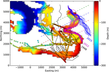
Fig. 10. Bathymetry at the front of Eqip Sermia. Depth soundings from a research vessel in 2014 and 2015 are shown with circles. Swath bathymetry data from Rignot and others (Reference Rignot, Fenty, Xu, Cai and Kemp2015) are shown as colored bands. Positions of the calving front in 1912, 1920, 1929, 1948, 2012 and 2015 are indicated with lines. The red circle marks the shallow area where a protruding ice cliff had formed (cf. Figs 1, 4).
The topographic influence of this shallow area is also manifested by the stepped and asynchronous retreat of the two lobes since 2000. For example, after the onset of retreat between 2000 and 2003, the retreat paused. Only in 2009 did the northern lobe (green and blue in Fig. 5) step back rapidly (~1.5 km), then stagnating in 2013. In contrast, the southern lobe (red and purple in Fig. 5) was stable until 2013 and then retreated rapidly by 1 km within one year (Fig. 3).
The current calving front position is unprecedented since historical observations started in 1912, and likely was never reached since the earliest maps by Rink (1853; Fig. 10 in Weidick and Bennike, Reference Weidick and Bennike2007) and by Engell (1902; Fig. 3 in Bauer, Reference Bauer1955) which, however, show only sketchy front positions similar to the 1912 extent.
Except for the most recent years, front position changes have been relatively moderate and slow, which may be a result of the relatively shallow water depth (<100 m) and wide lobate shape of Eqip Sermia at its maximum extent. Due to the wide cross-sectional area there, the frontal ice flux per unit area was much lower than at today's narrower terminus position, which is roughly half the width. Consequently, changes in ice flux likely had less influence on terminus height and length change than in the present configuration.
4.2. Velocity and geometry
Similar to the front position variations, surface flow velocities were relatively stable until very recently, certainly at the few times they were measured during the last century. Slight accelerations (~30%) were recorded between the 1940s and 1970s, when the terminus also advanced slightly (Fig. 6a). Even after the first step retreat in 2001, and until 2005, flow speeds remained at levels similar to 1912. Until 2011, the protruding lobate tongue remained intact (Figs 4, 6) with a surface elevation profile almost identical to 1959 and only slightly lower than in 1948. Thus, the surface slope and therefore the stress state at the terminus were probably very similar, explaining the unchanged flow speeds and calving rates.
The flow velocities show a clear seasonality with speedup approximately coinciding with the beginning of the melt season, and slowdown in late summer (Fig. 7). This velocity variation amounts to ~10% of the flow speed in the near-terminus parts. The observed velocity variations might reduce the significance of the episodic historic measurements of flow speeds. Even if all of these measurements were taken in summer, different timings and varying seasonality render the measured values only approximately comparable.
On a seasonal scale, Eqip Sermia behaves in a manner similar to other outlet glaciers of the GrIS (Howat and others, Reference Howat, Box, Ahn, Herrington and McFadden2010; Moon and others, Reference Moon2014). It fits into the standard category of seasonal speedup, with acceleration at the beginning of the melt season, and deceleration to the same or slightly lower velocity at the end of the melt season (categories 2 and 3 in Moon and others, Reference Moon2014). Due to the limited temporal resolution available, the exact cause of these seasonal speedups is difficult to assess, but enhanced basal motion due to surface meltwater, as well as changes in the terminus geometry and ice mélange conditions in the fjord may play a role (Howat and others, Reference Howat, Box, Ahn, Herrington and McFadden2010). The absolute seasonal speed increase over the lowest 15 km of the glacier is approximately constant (Fig. 7), which might be a sign of processes on the ice sheet. Meltwater induced variations of basal motion during the summer have been observed on the nearby ice sheet, with basal motion as the dominant contribution to surface velocity throughout the year (Andrews and others, Reference Andrews2014; Ryser and others, Reference Ryser2014b). It is likely that similar processes influence the seasonal acceleration of this outlet glacier, and that stress transfer to the base is weak in large portions of the terminus area with bedrock far below sea level (Fig. 6b). Such a setting would then lead to plug-like ice flow, which is dominated by horizontal stress transfer through the ice to strongly coupled areas (Ryser and others, Reference Ryser2014a) such as the shallow sill under the present terminus of Eqip Sermia.
After the most recent major step retreat starting in 2010, the flow accelerated substantially in 2012/13 to about twice its previous long-term speed and sped up further in 2014 to 12 m d−1 (blue and red dots in Figs 6a, 8a). This strong and sudden acceleration coincided with the collapse of the relatively flat protruding terminus, which resulted in a much steeper and higher calving front, higher longitudinal stresses and extensional strain rates, and consequently faster flow at the terminus. In the central part of the glacier this cliff attained a height of 150–200 m at a slope angle exceeding 45° (Figs 8b, 9). A bedrock height beneath the northern half of the terminus reaches almost to sea level in places (visible beneath cliff at low tide; Fig. 9) and may explain the steepening of the ice surface at this location (Figs 6b, 8b) and the recent formation of the very high ice cliff. Interestingly, the highest velocities were measured at the bottom of this cliff (Fig. 8a) and are likely due to bulging and extrusion caused by the stress state in such a steep geometry (Hanson and Hooke, Reference Hanson and Hooke2000; Leysinger–Vieli and Gudmundsson, Reference Leysinger–Vieli and Gudmundsson2004). Angles and velocities were considerably lower on the southern lobe of the terminus with much lower cliff height (purple in Fig. 8).
A 200 m high ice cliff above water is, to our knowledge, exceptional for ice-sheet outlet glaciers, for which heights of <100 m are conventionally assumed (e.g. Bassis and Walker, Reference Bassis and Walker2012; Pollard and others, Reference Pollard, DeConto and Alley2015). This high ice cliff is also special regarding its surface slope and setting. While most cliffs are close to vertical, and often floating or close to flotation, the high cliff observed at Eqip Sermia in 2014 is inclined with a slope angle exceeding 45° (Figs 8b, 9) and rests on very shallow bedrock.
The current special geometric situation of the 200 m high, steep ice cliff on the central to northern part of the front (blue profile in Fig. 8b) may also explain the new phenomenon of large tsunami waves that are triggered by subaerial collapses of the ice front with volumes of the order 105 m3 (one such event is investigated in detail by Lüthi and Vieli, Reference Lüthi and Vieli2015). These large tsunami waves cause wave run-ups at the opposite shore of 15–20 m height. Indeed, the geometric situation of the very high and steep ice front since 2012 coincides with the start of tsunami related problems in the landing of boats at the ‘Camp Eqi’ tourist operation. This was also the beginning of active erosion of vegetation and soil along the shore up to 20 m a.s.l. This soil with mosses and dwarf shrubs and a thickness of 20–30 cm is likely hundreds to thousands of years old, given the very short growing season in the Arctic and the resulting slow biomass production. Therefore, the very recent erosion of these soils indicates that the current setting of the terminus with a very high calving cliff is unprecedented during the past hundreds, and possibly few thousands of years.
4.3. Comparison with other regions in West Greenland
The terminus position history at Eqip Sermia is in rough agreement with other tidewater outlet glaciers in West Greenland, at least at a decadal timescale. The trend with reduced glacier extents in the 1940–50s, and a readvance thereafter, has been recorded at several smaller outlet glaciers (Fig. 60 in Weidick and Bennike, Reference Weidick and Bennike2007), whereas some big glaciers show step-like retreat without full readvance (e.g. Upernavik Isstrøm, Umiammakku Glacier, Rink Isbrae, Jakobshavn Isbrae, Kangiata Nunata Sermia). Similar to Eqip Sermia, most regions around Greenland, particularly in the southwest, showed a slight advancing tendency between 1972 and 1985, stable positions between 1985 and 2000, and rapid retreat between 2000 and 2010 (Howat and Eddy, Reference Howat and Eddy2011; Lea and others, Reference Lea2014). In Southwest Greenland, the advancing tendency likely started even earlier (1960s; Warren and Glasser, Reference Warren and Glasser1992). For the North-West of Greenland, however, phases of major mass loss and retreat were concentrated around 1985–93 and 2005–10, and were related to short-lived dynamic ice loss events, rather than longer-term changes in surface mass balance, suggesting a link between these changes and ocean forcing (Kjær and others, Reference Kjær2012). Their phase of mass loss in the 1980s does, however, not quite agree with the period of stable terminus positions at Eqip Sermia at that time.
Although there seems to be a general agreement with trends in terminus changes at other tidewater outlet glaciers in West Greenland, the exact timing of these changes differs. For example, for Jakobshavn Isbrae, which is located only 70 km south of Eqip Sermia, the onset for rapid retreat and acceleration was in 1997 (Sohn and others, Reference Sohn, Jezek and Van der Veen1998; Joughin and others, Reference Joughin2008b), whereas the southern part of Eqip Sermia only started to retreat slowly after 2000 and stabilized after 2004, with further rapid retreat of the whole terminus only after 2009. Overall, Eqip Sermia's short-term detailed retreat pattern is rather distinct from other glaciers in the region, and seems strongly influenced by effects of the basal topography.
4.4. External forcing
Terminus positions of tidewater glaciers are influenced by a range of external processes and forcings (Carr and others, Reference Carr, Stokes and Vieli2013; Straneo and others, Reference Straneo2013): enhanced calving through submarine melting at the terminus by advected relatively warm ocean water; surface melting due to varying air temperature and radiation causing terminus thinning; enhanced crevasse opening through meltwater ponding and penetration in crevasses and consequently higher calving rates (Benn and others, Reference Benn, Warren and Mottram2007), and reduction of the calving process through ice mélange in the proglacial fjord, in particular on seasonal timescales (Joughin and others, Reference Joughin2008a; Amundson and others, Reference Amundson2010). Enhanced surface melt may further lead to a reduced mass balance in the feeding area upstream and thus reduce ice flux to the front. Geometric controls on the ice fracture processes, such as terminus bathymetry and resulting flow dynamics, further alter the response of the terminus to external forcing.
Below we discuss the observed evolution of terminus geometry and ice flow in the context of atmospheric and oceanic forcing, although for the latter the available record is very limited. Potential forcing from sea ice and ice mélange is not discussed here as no pertinent time series is currently available for Eqip Sermia.
In Figure 11, we investigate the relation of terminus position to air temperature and local surface mass balance (SMB) at the ice-sheet margin and thus the potential influence from surface melt. Long term (1848-present) reconstructions of monthly temperature and SMB on the GrIS are taken from a gridded dataset (with 5 km spacing; Box and others, Reference Box2013; Box, Reference Box2013, we use version 2, Personal communication from J. Box, April 2015). For comparison with measured length changes, we use yearly SMB and summer (JJAS) temperature averaged over eight grid cells upstream of the terminus. Comparison with these time series (Fig. 11a) shows slow but clearly detectable glacier advance during periods of cooling just before the 1920s and during 1960–1990. After 1920, a strong warming occurred that was slightly reduced after 1935 until 1960, which coincides with an initially relatively rapid retreat that slowed in the 1930s. The recent increasing air temperatures and negative surface mass balances started in 1996 and slightly precede the rapid terminus retreat beginning in 2000 and accelerating after 2010. Air temperatures continued to increase and SMB to decrease, reaching present levels, which are unprecedented within the reconstructions since 1848.
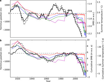
Fig. 11. (a) Eqip Sermia terminus position variations from Figure 5 (colored curves) are compared with long-term temperature reconstruction (7 a running mean; black solid curve) and SMB (black dashed curve), inverted for ease of comparison. (b) Same plot, but comparison with cumulative temperature and SMB. (Data from Box and others, Reference Box2013; Box, Reference Box2013).
Figure 11b shows that a more direct relationship regarding timing and amplitude is obtained by comparing length changes with detrended integrals of surface temperature and SMB (such integrals are often referred to as cumulative degree days and cumulative mass balance). Timings for the onset of phases of mass loss or mass gain and glacier advance and retreat are similar, and the recent rapid retreat coincides with increased warming since 2000. The agreement with integrals of summer temperature and SMB may reflect the cumulative action of these quantities on the glacier geometry. These findings could be interpreted such that the terminus position of Eqip Sermia is mainly controlled by the mass flux from the ice sheet rather than by processes at the terminus. However, the surface profile in 2008 is still almost identical to the one in 1959 and no substantial thinning in the upstream basin (behind the 2013 position) is apparent in Figure 6. Further, flow acceleration seems to propagate from the terminus inland rather than slow down from an upstream direction, as would be expected for a reduced upstream mass flux. Alternatively, and probably more likely, the more negative SMB and higher temperature could simply have thinned the terminus, which approached flotation, thereby increasing calving rates and causing retreat (Van der Veen, Reference Van der Veen1996). Acceleration in flow would then be the consequence of a dynamic feedback (Pfeffer, Reference Pfeffer2007).
Only very few records of ocean related forcing are available, in particular over the longer-term past, and they are not in close proximity of Eqip Sermia. The longest record is from Fylla Bank a few kilometers off the coast from Nuuk in West Greenland, consisting of yearly depth profiles in temperature and salinity measured in June (Andresen and others, Reference Andresen2012; Ribergaard, Reference Ribergaard2014). This record started in 1945 and for the depth of 0–40 m has been extended back to 1876 (Fig. 12c, blue lines). The ocean temperature records going down to 400 m at this location only start in 1945 but show very similar trends (Ribergaard, Reference Ribergaard2014). A reconstruction of gridded sea surface temperature (SST) in the Disko Bay area (average of 40 grid points) extending back to 1870 (Rayner and others, Reference Rayner2003) has also been considered. These two near-surface ocean temperature records are very similar (Fig. 12c) and show variations that resemble the summer (JJA) air temperatures in Ilulissat (Fig. 12b; from Cappelen, Reference Cappelen2014) and gridded temperature reconstructions from Eqip Sermia (Fig. 11), at least on decadal timescales. Again consistent with the length record (Fig. 12a) waters were relatively cold up to 1920 and from 1920 to 1935 substantially (2°C) higher temperatures were observed. Waters then remained relatively warm until the late 1960s when a substantial cooling was observed that fluctuated at decadal timescales until the late 1990s. Then, another warming of up to 2°C started, reaching the highest temperatures on record, only cooling slightly in 2007.

Fig. 12. (a) Eqip Sermia terminus position variations from Figure 5 (colored curves) are compared with (b) long-term measurements of summer (JJA) temperature at Ilulissat (red) and reconstructed summer temperature on the ice cap (black, same as Fig. 9; Box, Reference Box2013), (c) ocean temperature at 40 m depth at Fylla Bank (blue; Ribergaard, Reference Ribergaard2014), and SST reconstructions (from Rayner and others, Reference Rayner2003): JJA (red) and annual mean (orange), and (d) ocean temperature proxy from foraminifera (Lloyd and others, Reference Lloyd2011). Note that the temperature scales are inverted for ease of comparison.
For the deeper fjord waters, single annual depth profiles down to 300 m depth from Disko Bay since 1980 (Ribergaard, Reference Ribergaard2014) and trawl fisheries data (150–600 m depth) show that warm ocean water of Atlantic origin has been reaching Disko Bay since about 1997 (Holland and others, Reference Holland, Thomas, de Young, Ribergaard and Lyberth2008). This warm subsurface water was the likely trigger for the rapid disintegration of the floating terminus of neighboring Jakobshavn Isbrae (Sohn and others, Reference Sohn, Jezek and Van der Veen1998), which subsequently accelerated and retreated at a rapid rate (Joughin and others, Reference Joughin2008b). A similar ocean temperature signal has been derived from foraminifera within Disko Bay (Fig. 12d; Lloyd and others, Reference Lloyd2011). This record shows a marked increase in water temperature in the 1990s, and also seems to slightly precede the terminus position retreat signal of Eqip Sermia, but there are large uncertainties in timing in this proxy record due to approximate dating. Although these longer-term trends in oceanic conditions are generally consistent with retreat at Eqip Sermia, the available subsurface ocean data are distant and therefore not necessarily representative for oceanic conditions at the calving front of Eqip Sermia. Further, the bathymetry at Eqip Sermia is shallow (<100 m), which may prevent the warm subsurface water from reaching the calving front.
Recent local oceanic measurements from August 2014 (Beaird and others, Reference Beaird, Straneo and Jenkins2015) show that the warm Atlantic waters are present at depth in Ata Sund, but at least in late summer, they stay below 200 m depth. Due to the shallow water depths and sills at Eqip Sermia and its slightly deeper northern neighbor, Kangilerngata Sermia, these Atlantic waters do not directly reach the calving front of Eqip Sermia. Instead, these ice fronts are in contact with polar waters, which are higher in the water column and are substantially colder (1–2°C potential temperature). These waters are influenced by seasonally warmed polar warm waters and can be linked to the long-term near-surface record at Fylla Bank in Figure 12b. Tracer analysis of noble gases collected in Ata Sund (Beaird and others, Reference Beaird, Straneo and Jenkins2015) indicates strong upwelling driven by buoyancy of submarine meltwater and subglacial runoff from surface melt. The so determined ratio of submarine meltwater to surface melt runoff exceeds 25%. This implies that despite a lack of access to the deeper warm Atlantic waters, substantial rates of oceanic melt can occur at these calving fronts as estimated previously for the summer of 2008 (Rignot and others, Reference Rignot, Koppes and Velicogna2010). Using a very conservative estimate of subglacial discharge of 10 m3 s−1 (more than an order of magnitude below mean August estimates used by Rignot and others (Reference Rignot, Koppes and Velicogna2010)), and assuming a 3 km by 80 m deep submerged cliff face area, would at Eqip Sermia result in an average submarine melt rate of the order of 1 m d−1. Observations at other calving fronts in relatively shallow Greenlandic fjords support this role of subglacial discharge for submarine melt at relatively shallow calving fronts (Fried and others, Reference Fried2015).
Thus, despite the relatively shallow water depth at Eqip Sermia, oceanic melt has the potential to affect calving and terminus retreat. It is, however, important to note that these local oceanic studies provide only single snapshots in time and a better understanding of temporal variability and trends is needed in order to better constrain the role of oceanic forcing on long-term behavior at Eqip Sermia.
Overall, comparisons with different types of records in Figure 12 suggest that oceanic forcing is as likely a candidate for causing the terminus changes of Eqip Sermia as atmospheric forcing. A similar conclusion was reached by Lea and others (Reference Lea2014) for Kangiata Nunata Sermia (southwest Greenland). Our inability to uniquely relate length changes to atmospheric or oceanic forcing suggests there is likely not one single cause. Indeed, the atmosphere and ocean are intrinsically coupled, and it therefore appears elusive to identify one single or dominant forcing for terminus changes at Eqip Sermia. This claim is further supported by the coupling between enhanced subglacial meltwater discharge due to atmospheric warming and increasing oceanic melt at the calving front through the mechanism of buoyancy driven convection (Straneo and others, Reference Straneo2013).
The future evolution of Eqip Sermia will likely be strongly controlled by the bed topography and calving dynamics rather than ice flux from the ice sheet, while the role of oceanic forcing remains uncertain. It is likely that the glacier, upon loss of contact with the shallow pinning points where the steep cliff is currently based, will recede into a deep upstream basin (Fig. 6b). There, the glacier bed is 200–400 m below sea level for 10 km until it reaches an area of up-sloping bed. Given the known calving glacier instability (e.g. Pfeffer, Reference Pfeffer2007; Nick and others, Reference Nick2013) we expect Eqip Sermia to retreat at substantial rates during the next decade.
5. CONCLUSION
Comparing a century-long record of terminus positions and ice velocities of Eqip Sermia with time series of atmospheric and oceanic forcing shows that the terminus position of this glacier varies in a manner similar to both forcings on a decadal timescale. It therefore seems problematic to discern whether the dominant forcing is altered mass balance on the ice sheet or varying ocean temperatures in the proglacial fjord providing energy for submarine melt. This distinction is complicated, as these two forcings are interlinked, with oceanic melt partly driven by subglacial meltwater discharge, which itself is a function of surface temperature.
Nevertheless, this unique, century-long record of outlet glacier behavior clearly shows that the current rapid retreat of Eqip Sermia is unprecedented on a century timescale. An almost century long phase of relative stability was abruptly terminated around 2000 with the onset of a very rapid, stepped retreat and a strong flow acceleration in the past few years. Eqip Sermia thus follows the recent rapid retreat of many Greenland outlet glaciers but exhibits particular dynamics that are likely controlled by the geometry of the glacier, the bed topography and the bathymetry of the proglacial fjord.
The stable terminus geometry of Eqip Sermia, compared with other Greenland outlet glaciers, is controlled by a shallow (<100 m) terminus area that supported the glacier during the past century. This is likely to change in the near future, as the glacier terminus will retreat into a bedrock depression with depths reaching 400 m below sea level. The terminus is likely to stabilize only 10 km behind the present position on upsloping bedrock. As many of the marine outlet glaciers of the GrIS will become landlocked, the mass flux will be reduced, stabilizing the ice sheet, albeit within a considerably smaller perimeter.
ACKNOWLEDGEMENTS
We thank the 2014 Advanced Climate Dynamics Summer School and the Danish Polar Station for ship-time on the Porsild research vessel. We further thank the crew, Kerim Nisancioglu, Fiamma Straneo, Nick Beaird and Rebecca Jackson for support of our oceanographic work, and Rémy Mercenier and Christoph Rohner for help in the field. Logistical support by World of Greenland, Flemming Bisgaard and the Ilulissat Water Taxi is acknowledged. Eric Rignot provided bathymetry data. We acknowledge the use of data products from CReSIS generated with support from NSF grant ANT-0424589 and NASA Operation IceBridge grant NNX13AD53A. SPOT-5 DEMs were provided at no cost by the French Space Agency (CNES) through the SPIRIT International Polar Year project (Korona and others, 2009). We thank Jason Amundson and two anonymous reviewers for careful reviews which improved the presentation, and editor Jo Jacka for the editorial work. This work was funded by the Swiss National Science Foundation Grant 200021_156098.


 Open access