


1. Introduction
The Greenland ice sheet is the second largest body of ice on Earth and it has the potential to contribute $7.4$ m to sea level rise if melted entirely (Intergovernmental Panel on Climate Change, 2014; Morlighem and others, Reference Morlighem2017). Over the last three decades, its ice mass loss rate doubled, increasing from $119$
 Gt a$^{-1}$
 over the period 1992–2011, to $244$
 Gt a$^{-1}$
 over the period 2012–17 (Shepherd and others, Reference Shepherd2020), making it responsible for $\sim$ $15$
$15$ % of the observed contemporary sea level rise (Cazenave and others, Reference Cazenave2018). Of the total ice sheet mass loss, more than $50$
 % can be attributed to surface mass balance ($55 \pm 5$
 % between $1998$
 and $2018$
 , Mouginot and others (Reference Mouginot2018); $68$
 % between $2009$
 and $2012$
 , Enderlin and others (Reference Enderlin2014)), which is becoming increasingly more negative (Mote, Reference Mote2007). Melt events and melt areal extent have expanded to higher elevations (Tedesco, Reference Tedesco2007; Fettweis and others, Reference Fettweis, Tedesco, van den Broeke and Ettema2011), reaching areas of the percolation and dry snow zone that previously experienced only little to no melt. This led to significant changes in the firn structure, such as the formation of thick impermeable ice layers in the lower percolation zone (Machguth and others, Reference Machguth2016). These ice layers have impeded meltwater percolation, causing meltwater to directly runoff and increasing the total ice sheet runoff area by $26\percnt$
 since 2001 (MacFerrin and others, Reference MacFerrin2019).
In order to better quantify and understand the ice sheet's contribution to sea level rise, it is thus fundamental to better constrain surface melt, which ultimately controls the surface mass balance and changes in the firn structure. Regional climate models (RCMs) such as the Modele Atmospherique Regionale (MAR) (Fettweis and others, Reference Fettweis2017), the HIRHAM RCM (Christensen and others, Reference Christensen2006) and the Regional Atmospheric Climate Model (RACMO2) (Noël and others, Reference Noël2018) are typically used to model the surface mass balance over the entire ice sheet. These are forced by either global atmospheric reanalysis data or general circulation models, allowing for projections as well as simulations of the past. Because RCMs are computationally very demanding, they are typically run on grids with resolutions on the order of $\sim \! 10$ km, although higher resolutions (Noël and others, Reference Noël, van de Berg, Lhermitte and van den Broeke2019) and downscaled results (Noël and others, Reference Noël2016) are now becoming available.
However, small-scale local studies are needed to evaluate these large-scale models and investigate the physical processes in more detail. These studies typically use 1-D models of varying complexity, forced by in situ meteorological observations from automatic weather stations (AWSs), to quantify the surface energy balance and the resulting melt. These models have become more complex since their first applications in Greenland in the 1980s (Braithwaite and Olesen, Reference Braithwaite and Olesen1990; Greuell and Konzelmann, Reference Greuell and Konzelmann1994), and nowadays typically include modules that simulate subsurface processes such as firn temperature, meltwater percolation and refreezing and firn densification (Charalampidis and others, Reference Charalampidis2015; Vandecrux and others, Reference Vandecrux, Fausto, Langen, van As and Macferrin2018, Reference Vandecrux2020; Samimi and others, Reference Samimi, Marshall, Vandecrux and MacFerrin2021). Studies focused on different aspects such as energy-balance partitioning (Braithwaite and Olesen, Reference Braithwaite and Olesen1990; Greuell and Konzelmann, Reference Greuell and Konzelmann1994; Henneken and others, Reference Henneken, Bink, Vugts, Cannemeijer and Meesters1994; Van Den Broeke, Reference Van Den Broeke2008), seasonal and interannual variability (Van Den Broeke and others, Reference Van Den Broeke, Smeets and Van De Wal2011), surface meltwater discharge modeling (Van As and others, Reference Van As2012) and long-term changes in surface energy fluxes (Kuipers Munneke and others, Reference Kuipers Munneke2018; Huai and others, Reference Huai, van den Broeke and Reijmer2020). Most of the previous local surface energy-balance studies have been carried out at sites along the K-transect, a historical transect in the ablation zone east of Kangerlussuaq in southwest Greenland (Fig. 1), where the surface mass balance has been measured since $1990$ and several AWSs have recorded atmospheric conditions and radiative fluxes since $1993$
 (Smeets and others, Reference Smeets2018).
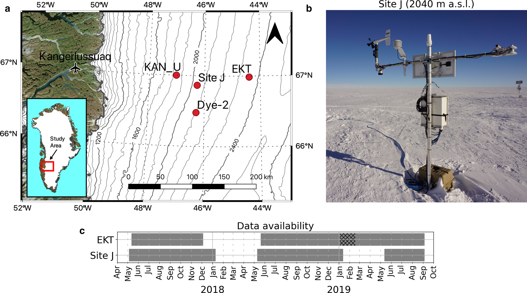
Fig. 1. (a) Study area and locations of sites relevant for this study; elevation contours in m a.s.l. are based on the ArcticDEM 1 km v.3.0 product by Polar Geospatial Center (Porter and others, Reference Porter2018) adjusted with the EGM2008 geoid offset (Pavlis and others, Reference Pavlis, Holmes, Kenyon and Factor2012). (b) The AWS at Site J in Spring $2017$ . (c) Weather stations data coverage at EKT and Site J; the hatched area between $4$
 January and $17$
 February $2019$
 at EKT shows a period during which the sonic ranger (SR50) was malfunctioning; data gaps are due to power failure; ticks refer to the first day of each month.
In contrast, energy-balance studies in the percolation zone are fewer and more recent. Charalampidis and others (Reference Charalampidis2015) modeled the surface energy balance at the KAN_U site (1840 m a.s.l., the highest site of the K-transect) during the period between $2009$ and $2013$
 , showing evidence of enhanced melt and reduction of the refreezing capacity of firn. Vandecrux and others (Reference Vandecrux, Fausto, Langen, van As and Macferrin2018) and Vandecrux and others (Reference Vandecrux2017) applied a multilayer firn model to study changes in the firn properties such as density and cold content at different sites in the percolation and dry snow zone of the Greenland ice sheet. Samimi and others (Reference Samimi, Marshall, Vandecrux and MacFerrin2021) combined modeling efforts with time-domain reflectometry measurements to monitor and constrain meltwater and refreezing processes at the Dye-2 site (2120 m a.s.l., southeast of KAN_U). However, none of these studies focused on assessing the model's ability to reproduce melt accurately. To our knowledge, a point energy-balance model, including radiation penetration and deep water percolation, has not been evaluated in detail in the percolation zone of the Greenland ice sheet.
In this study, we use data from two weather stations in the percolation zone in southwest Greenland to force a surface energy-balance model coupled to a multilayer subsurface model. We evaluate model results against independent observations of surface height, and surface and subsurface temperatures. We perform extensive experiments to assess model sensitivity to input forcings, model parameters and parameterizations. Furthermore, we account for the penetration of shortwave radiation into the snow, following the approach of Kuipers Munneke and others (Reference Kuipers Munneke2009, Reference Kuipers Munneke, van den Broeke, King, Gray and Reijmer2012), and deep water percolation, following the approach of Marchenko and others (Reference Marchenko2017), and we assess their impact on the surface energy balance and melt estimates.
2. Study area and observations
Two AWSs were installed during spring $2017$ at Site J ($2040$
 m a.s.l.) on $28$
 April and at EKT ($2360$
 m a.s.l.) on $6$
 May (Fig. 1a) and operated until $5$
 September $2019$
 . The sites are located in the southwest percolation zone of the Greenland ice sheet in proximity to the K-transect, $\sim$ $80$
$80$ km apart from each other and more than $150$
 km from the ice margin. Both sites have been subject to previous studies, including a $> \!200$
 m firn core drilled at Site J in $1989$
 (Kameda and others, Reference Kameda1995) and shallow firn core collection between $2013$
 and $2017$
 at EKT (Machguth and others, Reference Machguth2016; MacFerrin, Reference MacFerrin2018).
The stations recorded near-surface air temperature, relative humidity, wind speed and direction, shortwave incoming and reflected radiation, longwave incoming and outgoing radiation and relative surface height (Fig. 1b, Table I). Subsurface temperatures were measured at $28$ depths, with the first $23$
 thermistors spaced $0.5$
 m apart, and the next five thermistors spaced $1.0$
 m apart. The uppermost sensor was at a depth of $1$
 m below the snow surface at both sites during installation in spring $2017$
 . Two additional thermistors (Table I) were added in May $2019$
 at a depth of $0.45$
 and $0.70$
 m at Site J and $0.78$
 and $1.15$
 m at EKT. Meteorological variables were sampled every $5$
 min, while surface height and subsurface temperatures were sampled every hour. At Site J, the instruments were mounted to a $5$
 m long mast drilled initially $3$
 m into the firn and secured with three guy wires (Fig. 1b). At EKT, instruments were mounted to an already existing station (MacFerrin and others, Reference MacFerrin, Stevens, Vandecrux, Waddington and Abdalati2022). At both sites, instruments were installed $2$
 m above the surface in May $2017$
 and reset to $2$
 m in May $2018$
 to avoid instruments’ burial due to net accumulation. The instruments’ height above the surface varies between $1.25$
 and $2.18$
 m at Site J and $1.39$
 and $2.10$
 m at EKT. Due to power failure, the stations failed to record data during part of the winter; data availability is shown in Fig. 1c.
Table 1. AWSs’ instruments and accuracy
Additional firn temperature thermistors were deployed in May 2019 at Site J$^{a}$ and EKT$^{b}$
 .
.
The two data series have been quality-checked and corrected when necessary. The summer (June, Julyand August) mean air temperature ($T_{\rm air}$ ) was below freezing at both sites for all 3 years on record, ranging between $-6.2$
 and $-4.4^{\circ }$
 C at Site J and $-9.0$
 and $-6.9^{\circ }$
 C at EKT, with $2017$
 and $2019$
 being the coldest and warmest summers, respectively. Maximum air temperatures of $7.6^{\circ }$
 C at Site J and $6.1^{\circ }$
 C at EKT were measured during summer $2019$
 . Both relative humidity ($RH$
 ) and wind speed ($u$
 ) exhibit little interannual and spatial variability, with $RH$
 values between $84$
 and $86$
 % at Site J and $82$
 and $86$
 % at EKT and $u$
 values between $4.6$
 and $5.4$
 m s$^{-1}$
 at Site J and $3.9$
 and $5.0$
 m s$^{-1}$
 at EKT. Firn temperature ranges between $-18.7$
 and $0.0^{\circ }$
 C at Site J and between $-23.8$
 and $-2.4^{\circ }$
 C at EKT, with the maximum values recorded during summer $2019$
 . The average temperature ($\pm$
 SD) computed at depths $> \!10$
 m below the surface over the entire study period is $-13.4\pm 0.3$
 and $-19.3\pm 0.1^{\circ }$
 C at Site J and EKT, respectively. In close proximity to each station, an ablation stake was installed to allow independent measurements of relative surface height, useful to compare and validate the data from the sonic ranger. The relative surface height change over the whole study period (spring $2017$
 –fall $2019$
 ) was $+ 1.05$
 m at Site J and $+ 1.55$
 m at EKT.
The subsurface model used in this study was initialized with firn data from two $25$ m firn cores that were drilled at Site J and EKT in spring $2017$
 using a mechanical ice-coring drill. A detailed description of the firn cores is given in Rennermalm and others (Reference Rennermalm2012). Density data from close by snow pits were used for the winter snow layer, which ranged from $0.87$
 m at Site J to $0.90$
 m at EKT in $2017$
 .
.
3. Melt modeling
Here, we develop a 1-D surface energy-balance model that computes all relevant surface energy fluxes and resulting melt with hourly resolution. The model is largely based on the Distributed Energy BAlance Model (DEBAM) (Hock and Holmgren, Reference Hock and Holmgren2005), which includes a multi-layer subsurface model that computes subsurface temperature, density and water content (Reijmer and Hock, Reference Reijmer and Hock2008). A brief description of our model is given below. For further details we refer to Hock and Holmgren (Reference Hock and Holmgren2005) and Reijmer and Hock (Reference Reijmer and Hock2008).
3.1. Surface energy-balance model
The surface energy balance is calculated by:

where $S_{\rm in}$ and $S_{\rm ref}$
 are the incoming and reflected shortwave radiation, respectively, $L_{\rm in}$
 and $L_{\rm out}$
 are the incoming and outgoing longwave radiation, respectively, $H$
 is the sensible heat flux, $LE$
 is the latent heat flux, $Q_{\rm R}$
 is the energy supplied by rain, $Q_{\rm G}$
 is the energy flux into the subsurface (also referred to as ground heat flux) and $Q_{\rm M}$
 is the energy available for melt. Fluxes toward the surface are defined as positive. The model uses a skin layer formulation to close the energy balance at the surface. In this approach the surface is assumed to be an infinitesimal skin layer without heat capacity that reacts instantaneously to a change in energy input. Several fluxes in Eqn (1) directly depend on the surface temperature $T_{\rm s}$
 ($L_{\rm out}$
 , $H$
, $H$ , $LE$
 , $Q_{\rm G}$
 and $Q_{\rm R}$
 ). A bisection method is iteratively applied to find the $T_{\rm s}$
 that satisfy Eqn (1) assuming $Q_{\rm M} = 0$
 . If a positive surface temperature is found (indicating surface melt, i.e. $Q_{\rm M} \ne 0$
 ), $T_{\rm s}$
 is reset to zero, and the energy balance is recalculated. The resulting non-zero $Q_{\rm M}$
 is converted into melt.
The radiative fluxes $S_{\rm in}$ , $S_{\rm ref}$
 and $L_{\rm in}$
 are taken from observations at the weather stations. $L_{\rm out}$
 is calculated from the modeled surface temperature using the Stefan–Boltzmann law, assuming an emissivity of $1$
 . Measured $L_{\rm out}$
 is used for model validation.
The turbulent fluxes are calculated using the bulk aerodynamic method, relating $H$ and $LE$
 to wind speed and gradients of temperature and vapor pressure between the surface and the air (Hock and Holmgren, Reference Hock and Holmgren2005). Wind speed and air temperature are based on observations, and vapor pressure is calculated from measurements of relative humidity. For these calculations, we assume a constant measurement height above the surface of 2 m. The effect of atmospheric stability is taken into account using the Monin–Obukhov similarity theory. Stability functions for stable atmospheric stratification are computed following Beljaars and Holtslag (Reference Beljaars and Holtslag1991), while stability functions for unstable atmospheric stratification are computed following Panofsky and Dutton (Reference Panofsky and Dutton1984). Surface roughness length for momentum is set at a constant value of $10^{-4}$
 m, which is found to be a good assumption at these elevations on the ice sheet (Smeets and Broeke, Reference Smeets and Broeke2008a; Charalampidis and others, Reference Charalampidis2015). Surface roughnesses lengths for heat and moisture are calculated using the surface renewal theory (Andreas, Reference Andreas1987; Munro, Reference Munro1990).
The energy supplied by rain $Q_{\rm R}$ is determined by the rainfall rate and the temperature difference between the air and the surface (Hock and Holmgren, Reference Hock and Holmgren2005). The ground heat flux $Q_{\rm G}$
 is calculated from the temperature gradient between the surface and the first subsurface layer using Fourier's law and the thermal conductivity provided by the subsurface model. In this calculation, modeled surface temperature from the current time step and subsurface temperature from the previous time step are used.
3.2. Subsurface model
The subsurface model is based on the SOMARS model developed by Greuell and Konzelmann (Reference Greuell and Konzelmann1994) and further refined by Reijmer and Hock (Reference Reijmer and Hock2008). The model calculates firn temperature, density of the dry part of the firn and liquid water content on a vertical grid, including the effect of meltwater percolation, refreezing and dry firn densification. Here the grid extends from the surface to a depth of $25$ m with a total of $\sim$ $140$
$140$ layers with varying resolution: $0.05$
 m from the surface to $1$
 m depth, $0.1$
 m between $1$
 and $10$
 m depth and $0.5$
 m below $10$
 m depth.
First, the temporal evolution of the firn temperature is calculated using a forward time centered space finite difference method to solve the 1-D heat equation. Boundary conditions are given by the surface temperature at the snow surface, computed by the surface energy balance model, and by a constant temperature at the bottom of the firn column, determined by observations ($-13.4^{\circ }$ C at Site J and $-19.3^{\circ }$
 C at EKT). The thermal conductivity ($\kappa$
 ) is described as a function of the firn density, following the approach presented in Douville and others (Reference Douville, Royer and Mahfouf1995).
Next, if energy is available for melting ($Q_{\rm M} > 0$ ), the amount of melt at the surface is calculated. Meltwater and rainwater are then added to the liquid water content of the first subsurface layer. Refreezing, percolation and densification are sequentially calculated for every layer. The amount of refreezing is limited by either layer temperature, liquid water content or available pore space. If any water is still present in the layer, a small amount of it is retained in the layer against gravity due to capillary forces (irreducible water content) while the rest is allowed to percolate to the next layer. The irreducible water content is described as a function of the firn density, according to Schneider and Jansson (Reference Schneider and Jansson2004). Finally, the densification of the dry firn is calculated depending on the temperature gradient and the density following the Herron and Langway (Reference Herron and Langway1980) parameterization adapted by Li and Zwally (Reference Li and Zwally2004).
Solid precipitation is added to the first layer using observations of fresh snowfall thickness and density. The thickness for each time step was derived from total daily surface height changes in order to filter the often noisy sonic ranger data; daily values were then distributed equally over the day for the simulations. A fresh snowfall density of $350$ kg m$^{-3}$
 was derived from snow pit observations at Site J and EKT in Spring $2017$
 . This value reflects the rapid, wind-driven, compaction following snowfall events and it is in line with previous studies suggesting values between $315$
 and $400$
 kg m$^{-3}$
 for this area of the ice sheet (Charalampidis and others, Reference Charalampidis2015; Fausto and others, Reference Fausto2018; Vandecrux and others, Reference Vandecrux, Fausto, Langen, van As and Macferrin2018). The model does not account for the lateral flow of water. Subsurface layers are allowed to merge or split to maintain the initial grid configuration if they become thinner than $50$
 % or thicker than $150$
 % of their original thickness. This is often the case for the first layer, where thinning and thickening occur during melting and snowfalls.
3.3. Model application
The model was run at Site J and EKT from $6$ May $2017$
 to $4$
 September $2019$
 for all the periods when meteorological data were available (Fig. 1c). Hourly data of air temperature, relative humidity, wind speed, shortwave incoming and reflected radiation, longwave incoming radiation and solid precipitation provided the meteorological input to run the model. All the forcing inputs were taken directly from weather station observations. The model was run at $4$
 min resolution to assure the stability of the subsurface solver; hourly input data were linearly interpolated to match the required time step. The subsurface model was initialized with firn temperature and density data from the firn thermistor string and firn cores, respectively. When firn core data were unavailable (May $2018$
 at Site J and EKT, May $2019$
 at Site J), the firn density profile was initialized using model output from the end of that site's previous simulation adjusted to account for the correct seasonal snow depth.
3.4. Model validation
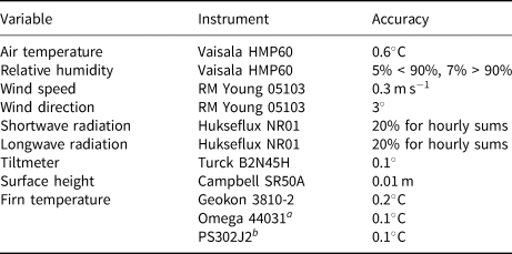
Simulations are validated against independent observations of relative surface height from both the weather station sonic ranger and ablation stakes readings (Fig. 2), surface temperature estimated from the measurements of outgoing longwave radiation using the Stefan–Boltzmann law with an emissivity of 1 (Fig. 2), and subsurface temperatures from thermistor strings (Fig. 3).
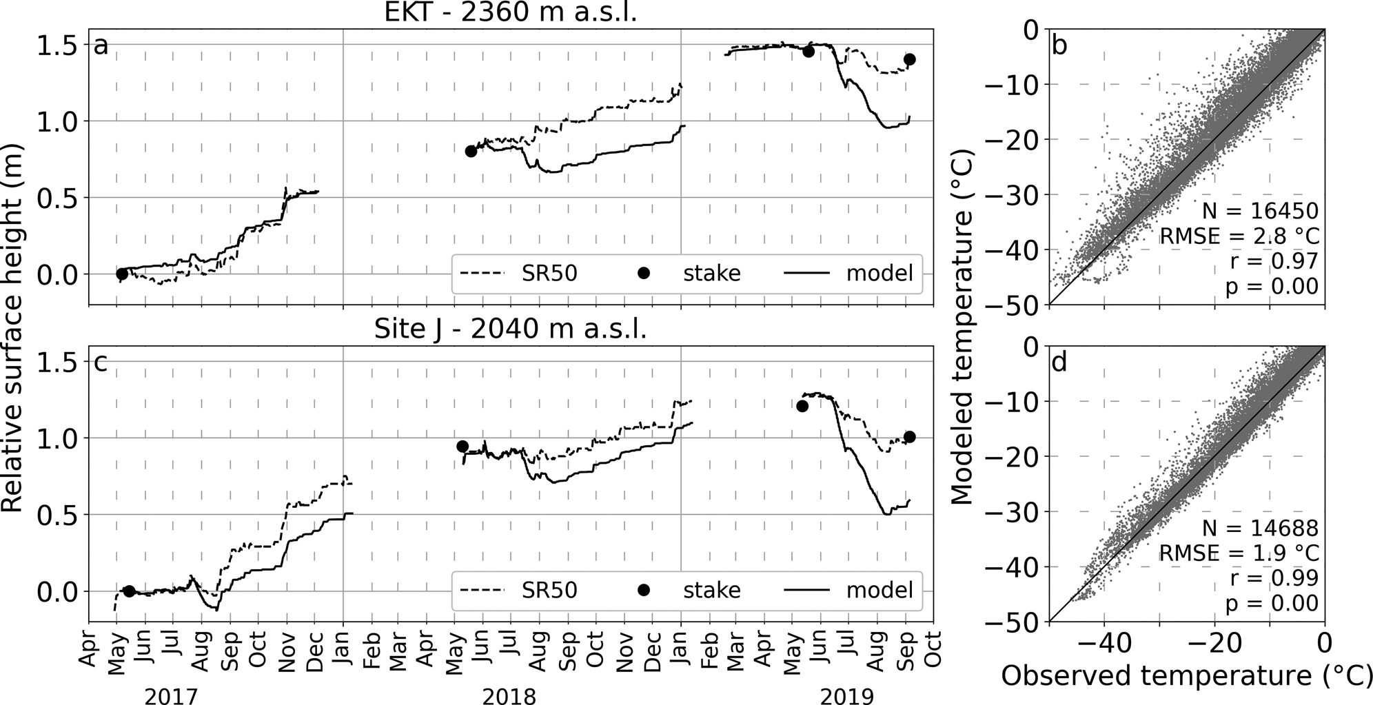
Fig. 2. Model validation at EKT (a, b) and Site J (c, d). (a, c) Modeled hourly relative surface height compared to measurements from the AWS sonic ranger (SR50) and ablation stake between May $2017$ and September $2019$
 . (b, d) Modeled vs observed hourly surface temperature, with the 1:1 line in black. ${N}$
 is the number of samples, RMSE the root mean square error, ${r}$
 the correlation coefficient and ${p}$
 the $p$
 -value.

Fig. 3. Hourly (a, d) measured, (b, e) modeled subsurface temperatures and (c, f) their differences for the uppermost 10 m between May $2017$ and September $2019$
 at EKT (a–c) and Site J (d–f). The depths are relative to the snow surface on the date of installation in early May $2017$
 . Black lines and black dots in (a, c, d, f) indicate the observed relative surface height and the thermistors position, respectively. Blue lines in (b, e) contour the boundary of subsurface liquid water. Gray lines in (b, e) indicate the depth of the uppermost thermistor. Data from the new thermistors installed in May $2019$
 are omitted in (a, c, d, f) when the sensors reached the surface or were affected by solar radiation penetration.
Independent in situ ablation stake readings, which provide relative surface height changes between annual field visits, match the continuous sonic ranger (SR50) data very well (Figs 2a, c). This provides confidence that the weather stations, where the sonic rangers were mounted, were not subject to sinking during the study period. In contrast, simulated relative surface heights do not agree well with these observations. Modeled surface lowering, almost entirely caused by melt, is consistently overestimated at both sites and during all three years except for EKT in summer 2017, where only little melt occurred. Maximum differences between observed and simulated relative surface height up to 0.47 m at Site J and 0.42 m at EKT are recorded during summer $2019$ when surface melting was most pronounced.
The comparison of modeled hourly surface temperatures with those derived from the measurements of outgoing longwave radiation reveals that the model tends to overestimate $T_{\rm s}$ , especially during the summer months when melt occurs at the surface (Figs 2b, d). The average difference between modeled and observed temperatures is $+ 1.11^{\circ }$
 C at EKT and $+ 0.59^{\circ }$
 C at Site J over the whole study period, increasing to $+ 1.93$
 and $+ 1.31^{\circ }$
 C, respectively when only the summer months (June, July and August) are considered. The correlation coefficient between hourly model results and observations is $0.97$
 and $0.99$
 , and root mean square error is $2.8$
 and $1.9^{\circ }$
 C at EKT and Site J, respectively.
Figure 3 shows simulated and observed subsurface temperatures and their differences. Temperatures below $-10$ m depth (not shown) remain constant at both sites and model results agree well with the observations. Simulated temperatures generally match the observations at depths below $4$
 m well, but the model tends to underestimate near-surface (between $0$
 and $4$
 m depths) temperatures during the winter and overestimate them during the summer (Figs 3c, f). The overestimation of summer temperatures is more evident in $2019$
 when melt was more pronounced. Furthermore, in May $2019$
 , two new thermistors were installed at both sites in that year's winter snow ($\sim$
 first meter), allowing for better validation of near-surface model results. Such observations were not available in $2017$
 and $2018$
 (first thermistors at $-1$
 m or lower), preventing us from validating model results closer to the surface in those years.
At both sites, modeled meltwater percolation (contoured by blue lines) did not reach the depth of the uppermost thermistor (gray lines) during the $2017$ and $2018$
 melt seasons (Figs 3b, e). During summer $2019$
 , modeled meltwater percolated much deeper than in the previous summers, reaching $-1$
 m at EKT and $-4$
 m at Site J. However, observations do not show the same thermal signal of percolating meltwater, typically characterized by the snowpack and firn becoming isothermal ($0^{\circ }$
 C). This results in large temperature differences (Figs 3c, f), with modeled temperatures up to $+ 13.9$
 and $+ 10.8^{\circ }$
 C warmer at EKT and Site J, respectively, during summer $2019$
 .
.
4. Model sensitivity
In this section, we investigate possible causes for the considerable differences between model results and observations highlighted above. We explore model sensitivity to input forcing and model parameters. Furthermore, we include a parameterization that accounts for shortwave radiation penetration into the snow and evaluate the impact on model results.
Henceforth, the simulations presented above are referred to as $sim\_ref$ . Because the sensitivity experiments at Site J and EKT portray an almost identical picture, for brevity and clarity, only results from Site J are presented here and discussed in detail. Results from EKT are summarized in the Supplementary material (Figs S5–S8).
4.1. Model forcings
The meteorological observations used to force the model can be prone to errors. Here we test how such errors could affect model results by homogeneously perturbing the five meteorological input variables one by one, and re-running the model with the new input forcings (Fig. 4). Applied perturbations are guided by instrument accuracy as declared by the manufacturer (Table I). For example, we perturb air temperature by $\pm 1^{\circ }$ C when the manufacturer stated accuracy is $0.6^{\circ }$
 C, etc. Furthermore, for each of the input variables, we explore a scenario that, on average, comes close to relative surface height observations (shown in orange in Fig. 4).
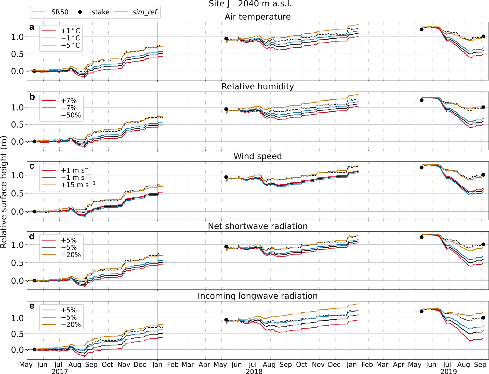
Fig. 4. Modeled hourly relative surface height compared to measurements from AWS sonic ranger (SR50) and ablation stake at Site J for simulations with different model forcings: (a) air temperature, (b) relative humidity, (c) wind speed, (d) net shortwave radiation and (e) incoming longwave radiation.
These experiments suggest that the discrepancies between the reference simulation and observations cannot be explained by errors in input forcing or instrument accuracy. The perturbations required to match the measured surface height are extreme and far from being physically reasonable, e.g.$-5^{\circ }$ C to air temperature, $-50$
 % to relative humidity, etc. Finally, given the large differences between model results and measurements, we are confident that not even the effect of combined perturbations (e.g. perturbing simultaneously two or more variables within reasonable limits) could explain the discrepancies.
Figure 4 indicates that, while positive perturbations typically produce more surface lowering, this is not the case for the wind speed. In fact, because turbulent fluxes at our sites are generally negative, higher wind speeds would cause more negative fluxes resulting in less surface lowering.
4.2. Model parameters and parameterizations
Model parameters and parameterizations (e.g. turbulent fluxes, thermal conductivity, etc.) used in the reference simulation are taken from the literature rather than calibrated to match the observations. To further investigate possible causes for the mismatch between model results and observations in $sim\_ref$ , here we test the model sensitivity to different choices of model parameters and parameterizations.
We perturb the surface roughness for momentum used in the reference simulation for the calculation of the turbulent heat fluxes ($z_{0m} = 0.1$ mm) by increasing and decreasing it by one order of magnitude (Fig. 5a). We change the new snow density from $350$
 kg m$^{-3}$
 to $300$
 and $400$
 kg m$^{-3}$
 (Fig. 5b). Thermal conductivity ($\kappa$
 ) determines subsurface temperature evolution; thus, it controls the ground heat flux calculation, ultimately affecting the surface energy balance. Several different parameterizations for thermal conductivity exist in the literature. Here we replace the one used in the reference simulation (Douville and others, Reference Douville, Royer and Mahfouf1995) with four others following Reijmer and Hock (Reference Reijmer and Hock2008): Van Dusen and Washburn (Reference Van Dusen and Washburn1929); Sturm and others (Reference Sturm, Holmgren, König and Morris1997); Östin and Andersson (Reference Östin and Andersson1991); Jansson (Reference Jansson1901) (Fig. 5c). Similarly, we replace the irreducible water content parameterization by Schneider and Jansson (Reference Schneider and Jansson2004) used in the reference simulation with the one presented in Coléou and Lesaffre (Reference Coléou and Lesaffre1998) (Fig. 5d). Finally, we turn off the densification parameterization (Fig. 5d).
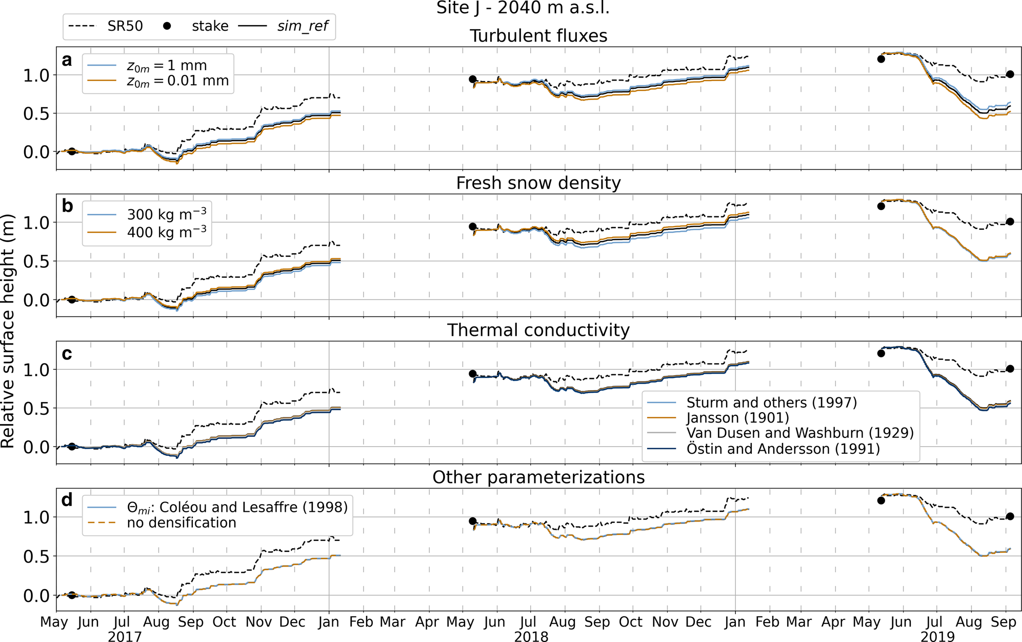
Fig. 5. Model sensitivity to choice of model parameters and parameterizations at Site J. Modeled hourly relative surface height compared to measurements from sonic ranger (SR50) and ablation stake for simulations with (a) perturbed roughness length for momentum and (b) perturbed fresh snow density, (c) different thermal conductivity and (d) densification and irreducible water content ($\Theta _{mi}$ ) parameterizations.
As evident from Figure 5, the model is not sensitive to these perturbations and changes. Differences to $sim\_ref$ are barely detectable in most cases. Changes in surface roughness for momentum by an order of magnitude only slightly change the simulations. It should be noted that because the model uses the parameterization by Andreas (Reference Andreas1987), surface roughness lengths for heat and moisture are computed as a function of $z_{0m}$
 ; thus, they are also affected by these perturbations.
While not directly affecting the surface energy balance, the fresh snow density parameter controls the conversion of melt into surface height change. Higher densities cause less surface lowering and vice versa. This is only noticeable when significant accumulation occurred before or during the melt season, e.g. in $2017$ and $2018$
 at Site J (Fig. 5b). Overall, simulation results are barely affected by the experiments. Thus, uncertainties in roughness lengths, snow density and thermal conductivity cannot explain the discrepancies between the reference simulation and observations.
4.3. Penetration of shortwave radiation
Although a well-documented physical process (e.g. Schlatter, Reference Schlatter1972; Colbeck, Reference Colbeck1989; Brandt and Warren, Reference Brandt and Warren1993), the penetration of shortwave radiation into the snowpack is not included in our model, consistently with most state of the art surface energy-balance models, including the most recent versions of RCMs such as MARv3.12, HIRHAM5 and RACMOv2.3p2 (Mankoff and others, Reference Mankoff2021). Few studies have investigated the effect of shortwave radiation penetration on the surface energy balance in Greenland (Van Den Broeke, Reference Van Den Broeke2008; Kuipers Munneke and others, Reference Kuipers Munneke2009) and in the Antarctic Peninsula (Kuipers Munneke and others, Reference Kuipers Munneke, van den Broeke, King, Gray and Reijmer2012). Here we use the same approach as Kuipers Munneke and others (Reference Kuipers Munneke2009), described in detail in the Appendix, to assess whether including this process in our model could explain the differences from the observations presented above.
The penetration of shortwave radiation, as described in this parameterization, strongly depends on the thickness of the fictitious surface layer, which is not to be confused with the thickness of the subsurface layers (see the Appendix for details and Kuipers Munneke and others (Reference Kuipers Munneke2009)). This calibration parameter controls the amount of net shortwave radiation ($S_{\rm net}$ ) that penetrates into the subsurface ($S_{\rm pen}$
 ) and the amount that is absorbed by the surface ($S_{\rm sfc}$
 ), affecting the surface energy balance and the warming of the subsurface. Here we present simulations using three different fictitious surface layer thicknesses: $0.01$
 , $0.05$
 and $0.25$
 m (Fig. 6). For small thicknesses, more shortwave radiation is allowed to penetrate into the subsurface while for thicker layers most of the shortwave radiation is absorbed by the surface: $S_{\rm pen} / S_{\rm net} = 43$
 , $17$
 and $4$
 % on average for the $0.01$
 , $0.05$
 and $0.25$
 m simulations respectively (Fig. 6c). If a very thick fictitious surface layer is considered all the net shortwave radiation would stay at the surface, replicating the assumptions made in the reference simulation when radiation penetration is not considered.

Fig. 6. (a) Hourly relative surface height, (b) annual cumulative total, surface and subsurface melt and (c) $30$ -day rolling average of shortwave radiation components ($S_{\rm net}$
 , $S_{\rm sfc}$
 and $S_{\rm pen}$
 ) for simulations including radiation penetration at Site J. Results using different fictitious surface layer thicknesses are presented: $1$
 cm in cyan, $5$
 cm in orange and $25$
 cm in red. Reference simulation in solid black and observations in dashed black. Reference simulation only has total cumulative melt and $S_{\rm net}$
 .
.
Both relative surface height and total melt vary very little from $sim\_ref$ (Figs 6a, b). This is because radiation penetration allows melting to happen also in the subsurface (e.g. firn temperature $= 0^{\circ }$
 C). Hence, the thinner the fictitious surface layers, the greater the melt in the subsurface layers, thereby compensating for less melt at the surface (Fig. 6b).
More details on the effects of radiation penetration are highlighted when looking at surface and subsurface temperatures. Figure 7 shows hourly temperatures for a 2 weeks period at Site J during the $2019$ melt season. During the first days, the near-surface snowpack is mostly temperate (i.e. at $0^{\circ }$
 C), indicating the presence of meltwater. Starting $28$
 June the air temperature drops resulting in a cooling of both the surface and the subsurface and an almost complete halt in melt. Surface temperature is higher for simulations with thicker fictitious surface layers, and it is the highest for the reference simulation (Fig. 7a), where radiation penetration is not considered. However, the simulated $T_{\rm s}$
 is higher than the observations for all the simulations. In contrast, subsurface temperatures, at both $0.1$
 and $0.25$
 m depth, are warmer for simulations with a thinner fictitious surface layer when more energy penetrates into the subsurface. Despite subsurface temperatures being sensitive to the choice of the fictitious surface layer thickness necessary to model the penetration of solar radiation, the experiments indicate that the omission of this process in the reference simulation cannot account for the differences between model results and observations.
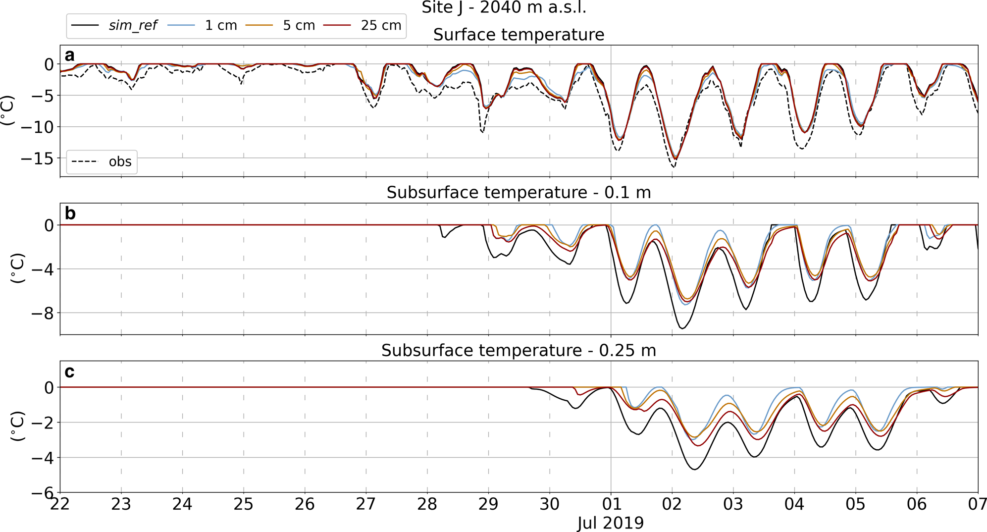
Fig. 7. Details of hourly surface temperature (a) and subsurface temperature at $0.10$ m (b) and $0.25$
 m (c) depth for simulations including radiation penetration at Site J for a 2 weeks period between the end of June and the beginning of July $2019$
 . Results using different fictitious surface layer thicknesses are presented: $1$
 cm in cyan, $5$
 cm in orange and $25$
 cm in red. Reference simulation in solid black and observations in dashed black.
4.4. Deep water percolation
Deep water percolation through preferential flow paths is a well-known process that affects water redistribution through the snow and firn matrix (e.g. Sturm and Holmgren, Reference Sturm and Holmgren1993; Humphrey and others, Reference Humphrey, Harper and Pfeffer2012; Cox and others, Reference Cox, Humphrey and Harper2015). However, this process is often not included in the subsurface models used in surface energy-balance models, which employ a tipping bucket approach to simulate water percolation from one layer to the next one. This is also the case for RCMs such as MAR, HiRAM and RACMO2. Marchenko and others (Reference Marchenko2017) used a simple statistical approach to parameterize deep water percolation, showing that accounting for this process improves the simulations of subsurface temperature.
Here, we apply the same approach, described in detail in the Appendix, to assess whether parameterizing deep water percolation could improve our model results presented above. Surface meltwater is redistributed to deeper subsurface layers following a probability density function that solely depends on a prescribed depth of maximum percolation (e.g. depth below which no water is allocated). Following Marchenko and others (Reference Marchenko2017), we test three different probability density functions, uniform (UNI), linear (LIN) and normal law (NORM), and three different maximum percolation depths, $2.5$ , $5.0$
 and $7.5$
 m.
m.
Accounting for deep water percolation reduces the $sim\_ref$ total melt at Site J over the entire study period between $1.4$
 and $9.7$
 %, depending on the probability density function and the maximum percolation depth used (Table S1). Surface melt is reduced the most when more water is redistributed from the surface to deeper subsurface layers (Fig. 8b). This is the case for simulations with deeper maximum percolation depths (e.g. $7.5$
 m) and using functions that allocate more water at depth (e.g.UNI). However, despite the decrease in melt, the relative surface height lowers more in these simulations than in $sim\_ref$
 (Fig. 8a). This is the result of redistributing meltwater and refreezing away from the surface. In a tipping bucket percolation model, in fact, the refreezing capacity of a layer is completely exhausted before water is allowed to percolate to the next layer. Thus, in $sim\_ref$
 refreezing rapidly increases the density of the surface layer making the surface lowering less compared to simulations with deep percolation. On the contrary, when water is allowed to percolate at depth, refreezing happens at multiple layers delaying the appearance of liquid water in the subsurface (Fig. S1) and keeping the density of the surface layer low.

Fig. 8. (a) Hourly relative surface height and (b) annual cumulative melt for simulations including deep water percolation at Site J. Results using different percolation probability density functions (UNI in cyan, LIN in orange and NORM in red) and depth of maximum percolation ($2.5$ m dotted, $5.0$
 m solid and $7.5$
 m dashed) are presented. Reference simulation in solid black and observations in dashed black.
The redistribution of refreezing at depth that follows deep water percolation also affect the subsurface temperature. All simulations overestimate the subsurface temperature at depths where water is allowed to percolate, showing larger temperature differences between model and observations compared to $sim\_ref$ (Fig. S2). Temperature differences are the largest for simulations that redistribute more water at depth, which are the same that also reduce melt the most.
These experiments indicate that, although accounting for deep water percolation slightly decreases melt, it makes the comparison with observations even worse than for the reference simulation.
5. Forcing the model with observed surface temperature
Surface temperature is a crucial variable used to determine several surface energy fluxes (Eqn (1)). Non-linear feedbacks when closing the energy budget with the skin layer formulation may cause errors in the modeled surface temperature. Therefore, we force the model with surface temperatures derived from measurements of outgoing longwave radiation. This experiment aims to evaluate the behavior of the model when the surface temperature is constrained by observations rather than modeled internally and to explore potential sources of errors responsible for the differences between model results and observations. Henceforth these simulations are referred to as $sim\_ T_{\rm s}^{\rm obs}$ .
.
Figure 9 shows that the simulated relative surface height matches well with the observations at both sites. Surface temperature observations cannot be used for validation since they are already used as input; however, we compare model results to subsurface firn temperature observations. In this experiment, modeled firn temperature (Fig. S3) compares better to thermistor string measurements than in $sim\_ref$ (Fig. 3). Maximum positive temperature differences are reduced from $+ 13.9^{\circ }$
 C at EKT and $+ 10.8^{\circ }$
 C at Site J for the reference simulations to $+ 6.54$
 and $+ 1.72^{\circ }$
 C. Furthermore, the meltwater percolation signal (e.g. isothermal firn $0^{\circ }$
 C) is better represented in this simulation. At EKT during the $2019$
 melt season, percolation never reached the depth of the first thermistor (gray line in Fig. S3b), consistent with observations. At Site J, during the $2019$
 melt season, simulated meltwater reached the depths of the first two thermistors consistent with the temperature observations (Fig. S3e). Total melt over the entire study period is $2.7$
 and $3.6$
 times smaller at Site J ($397$
 vs 1064 mm) and EKT ($217$
 vs 783 mm), respectively, for $sim\_ T_{\rm s}^{\rm obs}$
 compared to $sim\_ref$
 .
.
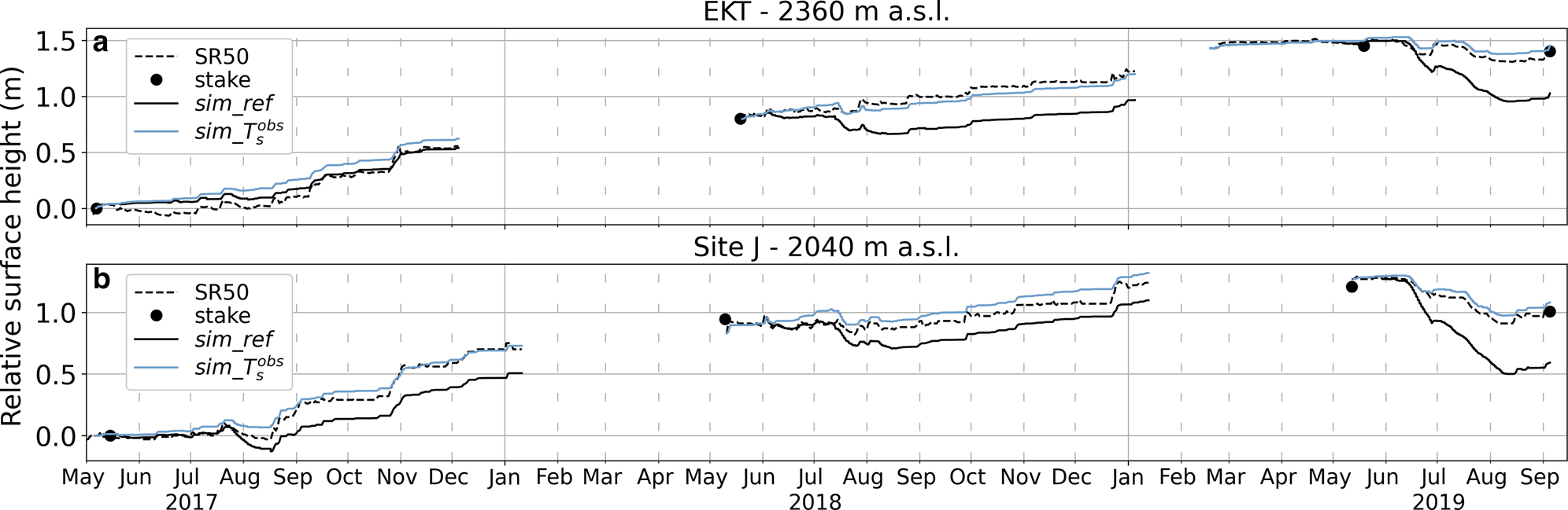
Fig. 9. Modeled hourly relative surface height compared to measurements from AWS sonic ranger (SR50) and ablation stake at (a) EKT and (b) Site J for simulations forced with observed surface temperature ($sim\_ T_{\rm s}^{\rm obs}$ ) and reference simulations ($sim\_ref$
 ).
).
Despite these results comparing well with observations, there are some underlying issues with these types of simulations. When the model is forced with observations of surface temperature all the fluxes in Eqn (1) are taken or computed from measurements. $S_{\rm in}$ , $S_{\rm ref}$
 , $L_{\rm in}$
 and $L_{\rm out}$
 are directly taken from observations. $H$
 , $LE$
 and $Q_{\rm R}$
 are computed as functions of observations. $Q_{\rm G}$
 is computed from measured surface temperature, previous time step subsurface temperatures and parameterized thermal conductivity. This causes a problem in the surface energy-balance closure. In fact, when melt is not occurring (e.g. $T_{\rm s} < 0$
 and $Q_{\rm M} = 0$
 ), the sum of all the fluxes may be different from zero. In contrast, when there is melt, the sum of all fluxes is always zero because the melt energy is set to be equal to the sum of all the other fluxes. This may lead to a negative computed $Q_{\rm M}$
 , which further underlines the problem in closing the energy balance. However, only this happens six times at Site J and three times at EKT with values of $Q_{\rm M} < 1$
 W m$^{-2}$
 .
.
At both our sites, the imbalance (Fig. 10) is non-negligible, with averages of $10.7$ and $6.1$
 W m$^{-2}$
 at EKT and Site J, respectively and daily means exceeding $50$
 W m$^{-2}$
 at times. Furthermore, the imbalance exhibits a clear seasonal signal at both sites. It is positive during the melt season and turns negative in winter, with greater magnitude during the summer (Fig. 10).

Fig. 10. Daily mean and $30$ -day rolling average of the imbalance in surface energy-balance calculations at EKT and Site J for simulations forced with observed surface temperature ($sim\_ T_{\rm s}^{\rm obs}$
 ).
).
6. Discussion
Simulated surface height changes at our two study sites match well with the observations when the model is forced with surface temperature ($sim\_ T_{\rm s}^{\rm obs}$ ) computed from observations of outgoing longwave radiation. However, when the skin layer formulation is used to close the surface energy balance ($sim\_ref$
 ), the model overestimates surface lowering and melt consistently during all three melt seasons. Sensitivity to both input forcings and model parameters has been extensively tested and cannot explain the differences between simulations and observations.
We also exclude insufficient accounting for firn compaction processes as possible cause for the discrepancy noting that our model includes a densification module although only considering dry firn. Also, our ablation stake and the SR50 both measure the thinning of the seasonal snow and firn layer between the base of the structure carrying the sensor and the surface, including both surface lowering due to melt and compaction. However, if compaction was underestimated the discrepancy between simulations and observations would be even larger. Furthermore, our conclusions are backed up by warmer surface and subsurface temperatures compared to observations.
6.1. Surface energy fluxes
Figure 11 shows the $30$ -day rolling averages of the surface energy fluxes for both $sim\_ref$
 and $sim\_ T_{\rm s}^{\rm obs}$
 at EKT (fluxes at Site J are shown in Fig. S4). $S_{\rm net}$
 and $L_{\rm in}$
 are identical for both simulations because they are taken from observations. $L_{\rm out}$
 and $LE$
 show small differences while larger discrepancies are found in $H$
 , $Q_{\rm G}$
 and $Q_{\rm M}$
 .
.
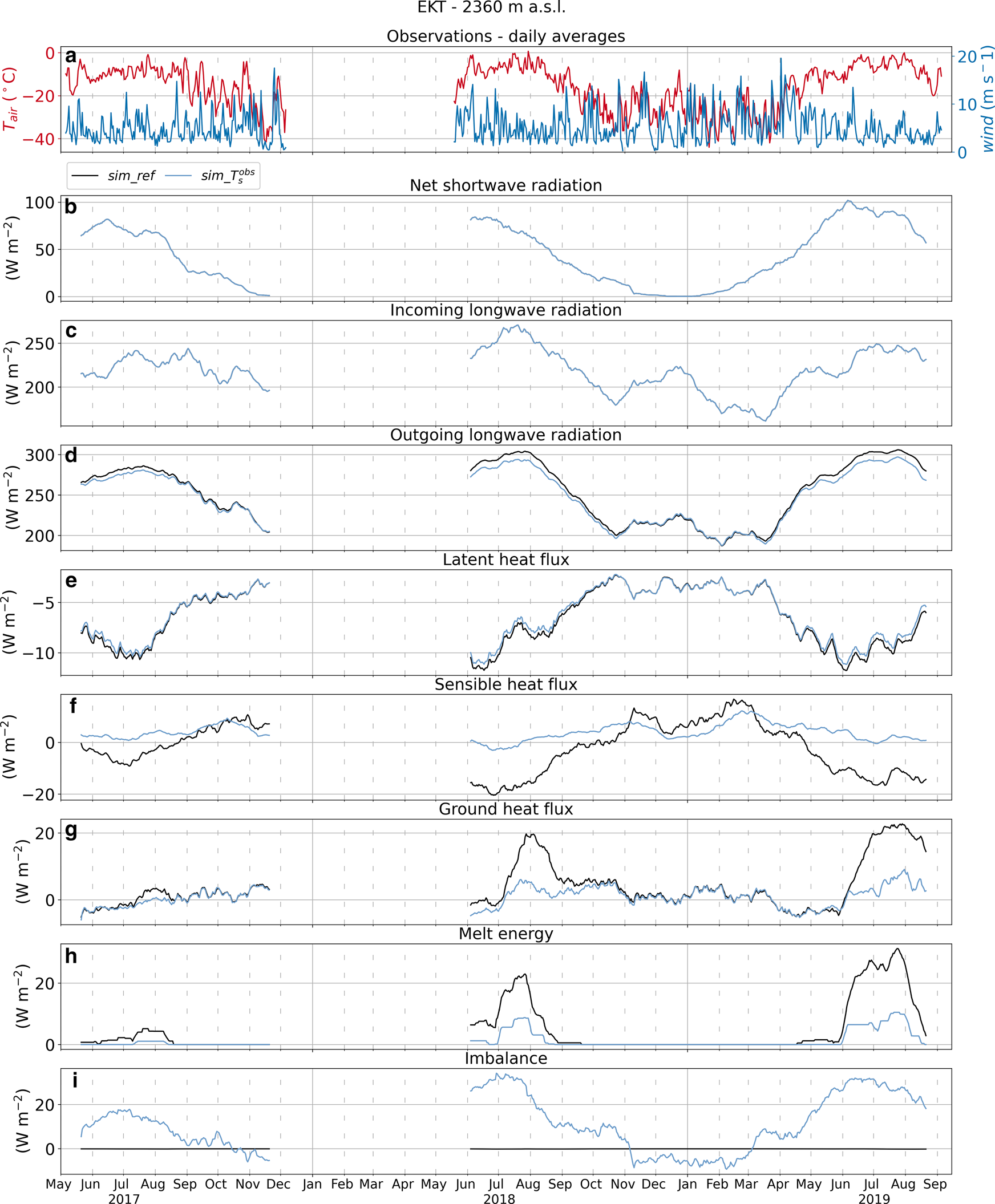
Fig. 11. Daily averages of air temperature and wind speed and $30$ -day rolling averages of surface energy-balance components for $sim\_ref$
 and $sim\_ T_{\rm s}^{\rm obs}$
 simulations at EKT: (a) air temperature and wind speed, (b) net shortwave radiation, (c) incoming longwave radiation, (d) outgoing longwave radiation, (e) latent heat flux, (f) sensible heat flux, (g) ground heat flux, (h) energy available for melt and (i) surface energy-balance residual.
Differences are generally small in winter but pronounced during the melt season. $H$ in $sim\_ref$
 is considerably more negative in the summer than $H$
 in $sim\_ T_{\rm s}^{\rm obs}$
 , which is mostly positive and small in magnitude (Fig. 11f). In contrast, $Q_{\rm G}$
 in $sim\_ref$
 is considerably more positive during the melting season compared to $sim\_ T_{\rm s}^{\rm obs}$
 (Fig. 11g). The few other studies modeling the surface energy balance at weather station locations in the percolation area of southwest Greenland (Charalampidis and others, Reference Charalampidis2015; Vandecrux and others, Reference Vandecrux2017, Reference Vandecrux, Fausto, Langen, van As and Macferrin2018; Samimi and others, Reference Samimi, Marshall, Vandecrux and MacFerrin2021) depict a similar picture to the one presented here, although simulated years are different. For example, Vandecrux and others (Reference Vandecrux, Fausto, Langen, van As and Macferrin2018) used the skin layer formulation and found that, on average, $H$
 was negative during summer. In contrast, Samimi and others (Reference Samimi, Marshall, Vandecrux and MacFerrin2021) forced their model with observations of surface temperature and $H$
 was generally positive during summer.
6.2. Surface temperature
$H$ and $Q_{\rm G}$
 strongly depend on surface temperature. $H$
 depends on the gradient between the air and the surface temperatures, while $Q_{\rm G}$
 depends on the gradient between the surface and the subsurface temperatures. Observations at our sites show that during the melt season surface conditions are characterized by a strong diurnal cycle (Fig. 12). The surface melts during the second half of the day and refreezes at night. Thus, the balance between the temperature of the air, the surface and the subsurface is delicate. Slightly different modeled surface temperatures can cause both $H$
 and $Q_{\rm G}$
 to change sign from negative to positive and vice versa, drastically changing the surface energy balance and modeled melt.

Fig. 12. Hourly air temperature from observations and surface temperature for the $sim\_ref$ and $sim\_ T_{\rm s}^{\rm obs}$
 simulations at EKT and Site J for the period between 7 and 17 July $2019$
 . The surface temperature for the $sim\_ T_{\rm s}^{\rm obs}$
 simulation is retrieved from observations of outgoing longwave radiation.
Figure 12 shows that the observed surface temperature used to force the $sim\_ T_{\rm s}^{\rm obs}$ simulation is lower than the modeled one in the $sim\_ref$
 simulation. Every time the air temperature (red line) falls between the observed ($sim\_ T_{\rm s}^{\rm obs}$
 ) and modeled ($sim\_ref$
 ) surface temperature, the $H$
 will differ in sign between the two different simulations, adding or subtracting energy available for the surface melt. The effect on the surface energy balance, however, is counterintuitive; in fact, the $sim\_ref$
 simulation, which overestimates melt, is the one exhibiting a negative $H$
 during the summer, which results in cooling of the surface (Fig. 11f). The $30$
 -day rolling average of $Q_{\rm G}$
 is positive for both simulations but much larger for $sim\_ref$
 , resulting in more energy directed toward the surface, allowing for more warming and more melting (Fig. 11g).
The effect of a slightly different modeled surface temperature is less pronounced for $L_{\rm out}$ and $LE$
 . $L_{\rm out}$
 directly depends on the surface temperature but not on its gradient with either the air or the subsurface; thus, it is not affected by the strong diurnal cycle described above. On the other hand, $LE$
 depends on the gradient between the air and the surface temperature, but its effect is filtered by the computation of the vapor pressure of the air and the surface.
Because these processes are non-linear, it is difficult to attribute the differences in melt between the two simulations to a particular flux. For example, $Q_{\rm G}$ is highly sensitive to warming of the subsurface through latent heat released by refreezing meltwater. This means that the larger $Q_{\rm G}$
 in the $sim\_ref$
 simulation may be a consequence of more melting and not the cause.
6.3. Closing the energy balance
Although the $sim\_ T_{\rm s}^{\rm obs}$ simulation captures surface lowering and melt during the summer well, results are inconsistent since the energy balance is not closed. The problem of surface energy-balance closure and residuals (Fig. 10) has been known for decades in the fields of boundary layer meteorology (e.g. Mauder and others, Reference Mauder, Foken and Cuxart2020). The imbalance has been attributed to neglected processes and uncertainties, typically assumed to be negligible for a horizontally uniform 2-D exchange surface without a canopy, with fluxes perpendicular to the surface. Although we are not aware of any mention in glaciological studies, Wang and others (Reference Wang2021) address this problem on seasonally frozen ground. They found that accounting for soil ice heat storage and latent heat of soil ice phase improved the estimates of the ground heat flux, reducing the imbalance. Our model currently treats the liquid water content in the subsurface separately from the dry part of the firn, perhaps accounting for liquid water heat storage would lead to a better representation of $Q_{\rm G}$
 .
.
Direct observations of the turbulent fluxes, e.g. using the eddy-covariance technique (Smeets and Broeke, Reference Smeets and Broeke2008b), and the ground heat flux are recommended by the boundary layer meteorology community to reduce the imbalance when investigating the energy-balance closure problem (Mauder and others, Reference Mauder, Foken and Cuxart2020). Unfortunately, such observations are rare in the percolation zone of the Greenland ice sheet. Furthermore, another process that is not included in our model and may affect the surface energy-balance calculations and closure is windpumping. Strong winds can disrupt the thermal regime of near-surface snow (Colbeck, Reference Colbeck1989) affecting $Q_{\rm G}$ . However, the sustained wind speeds required for this to happen are large ($> \!10$
 m s$^{-1}$
 ) and seldom recorded during the summer when the energy-balance residual is the largest (Figs 11a, i). Ultimately a better understanding of these problems will help improve our models, including when the skin layer formulation is used.
7. Conclusions
We applied an energy-balance model forced by weather station observations at two sites ($2040$ and $2360$
 m a.s.l.) in the percolation zone of the ice sheet over $3$
 years. Simulated melt and subsurface firn temperatures in summer were overestimated by the model compared to observations. The mismatch could not be explained by uncertainties in input forcings nor by choice of model parameters or various model parameterizations.
While the causes for the mismatch between simulations using the skin-layer formulation and observations remain elusive and need further investigation, our results highlight the complexity of energy-balance modeling in the percolation zone of the Greenland ice sheet. At these elevations, surface conditions during the summer are characterized by a strong diurnal cycle, with air temperatures barely above freezing. The surface melts and refreezes during melt days, and subsurface temperatures are modulated by the release of latent heat from refreezing water.
The mismatch is also of concern since RCMs, such as MAR, RACMO and HIRHAM, have used the same skin layer formulation to close the surface energy balance and compute the mass balance of the entire ice sheet (Christensen and others, Reference Christensen2006; Fettweis and others, Reference Fettweis2017; Noël and others, Reference Noël2018) and resulting contributions to sea level. Although RCMs being more complex than our model, e.g. they rely on parameterization also for the net shortwave radiation and incoming longwave radiation, our results suggest that melt estimates relying on the skin layer formulation may be biased and should be carefully evaluated and validated.
When our model was forced by observed surface temperatures, simulated surface height changes matched observations well; however, the energy balance is no longer closed, leaving unexplained residuals. The two different types of simulations, using the skin layer formulation and forcing the model with observed surface temperatures, yielded pronounced differences for the sensible and the ground heat flux, which both are directly dependent on the surface temperature. Due to pronounced diurnal cycles in surface temperature during the melt season, accurately modeling the surface temperature is crucial for reliable melt estimates in this region.
Better observations and measurements are needed to better understand the physical processes and mechanisms driving the surface energy balance in this area of the ice sheet. In particular, high-resolution temperature and moisture measurements of the near-surface seasonal snow would help to better constrain the role of the ground heat flux and the water content in the energy budget.
Processes such as the formation of impermeable ice layers are making the percolation zone increasingly more important in the mass budget of the Greenland ice sheet and a potential contributor to sea level rise. It is thus fundamental to further investigate the problems presented here to improve melt estimates of both point energy-balance models and the RCMs.
Supplementary material
The supplementary material for this article can be found at https://doi.org/10.1017/jog.2022.54.
Data
The weather stations’ data including firn temperature are available at https://www.doi.org/10.18739/A2BN9X444. Surface height data at EKT from MacFerrin and others (Reference MacFerrin, Stevens, Vandecrux, Waddington and Abdalati2022) are available at https://www.doi.org/10.18739/A25X25D7M. Firn cores density and stratigraphy are available at https://www.doi.org/10.18739/A2Q52FD98. The source code of the surface energy balance and subsurface model, including the penetration of shortwave radiation and deep water percolation parameterization, is available at https://github.com/fcovi/1D_SEB_model.
Acknowledgements
This study was supported by NSF grant no. 397516-66782. Polar Field Services provided logistical support for the field campaigns. The field measurements were assisted by Å. Rennermalm, C. Miege, I. Radivojevic, J. Kingslake, J. Xiao, K. Rogers, M. MacFerrin, P. Smith, S. Leidman and S. Munsell. Special thanks to M. MacFerrin for providing SR50 data from EKT and allowing us to attach instruments to his mast at EKT. We thank scientific editor William Colgan and two reviewers for their valuable reviews.
Author contributions
FC and RH developed the scope of the paper. FC performed the calculation and the analysis with the guidance of RH and CR. CR provided significant input on the development of the subsurface model. FC and RH conducted the fieldwork and collected the data in 2017–19. FC wrote the paper with input from RH. All authors commented on the manuscript.
Appendix A. Penetration of shortwave radiation
We compute the penetration shortwave radiation following the approach by Kuipers Munneke and others (Reference Kuipers Munneke2009), which is based on the method described by Brandt and Warren (Reference Brandt and Warren1993) and applied by Van Den Broeke (Reference Van Den Broeke2008). The parameterization employs the two stream approach from Schlatter (Reference Schlatter1972) to calculate the attenuation of shortwave radiation in the firn at different wavelengths.
First, the observed incoming shortwave radiation is divided into spectral bands using reference solar spectra from Brandt and Warren (Reference Brandt and Warren1993) and Kuipers Munneke and others (Reference Kuipers Munneke2009). In total $118$ wavelength bands from $299$
 to $2999$
 nm are used. Next the amount of shortwave radiation $S_{\rm pen}( z)$
 that penetrates to a depth $z$
 is given by the following equation from Schlatter (Reference Schlatter1972):

where $\lambda$ is the wavelength, $S_{\rm in}^{\lambda }$
 is the incoming shortwave radiation at given wavelength $\lambda$
 , $m_{\lambda }$
 is the multi-spectral albedo and $k_{\lambda }$
 is the multi-spectral extinction coefficient. Multi-spectral albedo and extinction coefficient are calculated following the approach of Brandt and Warren (Reference Brandt and Warren1993), using effective firn grain size, firn density and Mie scattering coefficients from Warren (Reference Warren1984), updated with values from Warren and others (Reference Warren, Brandt and Grenfell2006). Finally, the total shortwave radiation $S_{\rm pen}$
 that penetrates into the subsurface is calculated as $S_{\rm pen} = \sum ^{\rm layers} S_{\rm pen}( z)$
 , and $S_{\rm pen}( z)$
 is added to the respective subsurface layer. The surface energy-balance equation (Eqn (1)) becomes the following:


where $S_{\rm sfc}$ is the shortwave radiation absorbed by the surface, $S_{\rm net}$
 is the net shortwave radiation, $S_{\rm pen}$
 is the shortwave radiation that penetrates into the subsurface and the other variables are the same as in Eqn (1). Fluxes toward the surface are defined as positive.
For an infinitesimal surface layer, as it is the case for the skin layer formulation used in our model, all the net shortwave radiation would penetrate into the subsurface. To control the amount of $S_{\rm net}$ that penetrates into the subsurface ($S_{\rm pen}$
 ) and that is absorbed by the surface ($S_{\rm sfc}$
 ), previous studies (Van Den Broeke, Reference Van Den Broeke2008; Kuipers Munneke and others, Reference Kuipers Munneke2009) have attributed a fictitious thickness to the surface. This affects only the radiation penetration parameterization and is not to be confused with the layer thickness in the subsurface model. This fictitious surface thickness represents an important calibration parameter and sensitivity to it is discussed in detail in the ‘Results’ Section.
The evolution of the effective firn grain size required to compute multi-spectral albedo and extinction coefficients is modeled following the approach presented in Kuipers Munneke and others (Reference Kuipers Munneke2011). This method accounts for dry snow metamorphism, wet snow metamorphism, refreezing of liquid water and fresh snow. The effect of dry snow metamorphism is calculated using parametric curves from Flanner and Zender (Reference Flanner and Zender2006), while wet snow metamorphism is described by the parameterization presented in Brun and others (Reference Brun, Martin, Simon, Gendre and Coleou1989). The grain size of refrozen water is set to 1.5 mm following Kuipers Munneke and others (Reference Kuipers Munneke2011) while the grain size of fresh snow is set to $0.1$ mm based on snow pit observations at out study sites.
Appendix B. Deep water percolation
Following Marchenko and others (Reference Marchenko2017) preferential water flow to deeper layers in the snowpack and firn is simulated by redistributing surface meltwater among subsurface layers before refreezing is calculated. The amount of water allocated to each subsurface layer is determined by a probability density function PDF($z$ ,$z_{\rm lim}$
 ), where $z$
 is the layer depth and $z_{\rm lim}$
 is the user defined depth of maximum percolation. Three different PDFs are tested in Marchenko and others (Reference Marchenko2017) and included in this study as well.
PDF$_{\rm uni}$ describes uniform water infiltration. Water is redistributed equally to each subsurface layer between the surface and $z_{\rm lim}$
 :
:

PDF$_{\rm lin}$ describes linear water infiltration. Redistributed water linearly decreases with depth at a constant rate reaching $0$
 at $z_{\rm lim}$
 :
:

PDF$_{\rm norm}$ describes water infiltration following the normal law. Water is redistributed following the normal probability density function with SD $\sigma = z_{\rm lim}/3$
 , implying that $99.7$
 % of the water is allocated above $z_{\rm lim}$
 :
:


 Open access