


Introduction
It is common to observe crests of lateral moraines, trim lines and other features marking Neoglacial maxima in association with present-day glacier surfaces. Typically, the present surface and the former ice line indicated by these geomorphological markers converge up-glacier. This characteristic pattern indicates that thickness changes were largest in the lower reaches of glaciers. Reference WeidickWeidick (1968) has shown how the thickness change depends on altitude on local glaciers in West Greenland. However, quantitative aspects of the pattern have not been systematically investigated in other areas, even though it is an obvious and well-known feature of present-day glaciated mountain landscapes throughout the world.
There is some motivation for identifying any systematics in the variation of thickness change along the lengths of glaciers, which could simplify estimation of changes in ice volume. Volume is the crucial parameter for estimation of changes in water stored as glacier ice and contribution of glaciers to rising sea level (Reference MeierMeier, 1984). It is also related to the time-scale required for glaciers to complete their response to changes in climate (Reference PatersonPaterson, 1981; Reference Jóhannesson, Raymond, Waddington and OerlemansJóhannesson and others, 1989a), which Reference Jóhannesson, Raymond and WaddingtonJóhannesson and others (1989b) referred to as the memory length TM .
In order to relate changes in volume V of a glacier to changes in its length l Reference Jóhannesson, Raymond and WaddingtonJóhannesson and others (1989b) defined a profile-shape parameter

determined by thickness changes Δh relative to a reference glacier geometry of length l0
In this relation Δh(x, t) is the width-averaged thickness change at time t along the glacier length x running from 0 at the head to l at the terminus; Δh(l0,t) is the thickness change at the terminus of the reference glacier, and ![]() represents the average of Δh(x,t) over the length
represents the average of Δh(x,t) over the length ![]() . The parameter f may be viewed as a measure of the degree to which thickness changes are localized near the terminus Δh(l0,t) or spread evenly over the glacier length
. The parameter f may be viewed as a measure of the degree to which thickness changes are localized near the terminus Δh(l0,t) or spread evenly over the glacier length ![]() . It links the change in length l, which is related to Δh(l0,t) and the slope of the terminus (e.g. Reference NyeNye, 1960), and the change in volume, which is related to (Δh(x, t)) and the width distribution along the glacier length.
. It links the change in length l, which is related to Δh(l0,t) and the slope of the terminus (e.g. Reference NyeNye, 1960), and the change in volume, which is related to (Δh(x, t)) and the width distribution along the glacier length.
For a glacier of uniform width w, a volume change ΔV relative to the reference glacier may be expressed as
where ΔV(t) is the volume change between the head of the glacier and the reference terminus. Reference Jóhannesson, Raymond and WaddingtonJóhannesson others (1989b) used this result to show

where u(i0) is the velocity at the terminus of the reference glacier. Equation (3) is equivalent to a result predicted by Reference NyeNye (1960) with the additional content of a specific geometrical interpretation for the parameter f as expressed in Equation (1).
Based on models of kinematic wave propagation and diffusion, Reference NyeNye (1960) and Reference PatersonPaterson (1981) have suggested that characteristically ![]() , which corresponds to a near-linear variation of thickness change from near zero at the head to a maximum value at the terminus. Reference Jóhannesson, Raymond and WaddingtonJóhannesson and others (1989b) argued that f cannot be viewed as a separate independent parameter in Equation (3), but its value will depend, among other things, on the velocity of the terminus u(l) in such a way that TM
is not sensitive to the local terminus dynamics. Based on their flow models, they suggested that normally f should be less than ½.
, which corresponds to a near-linear variation of thickness change from near zero at the head to a maximum value at the terminus. Reference Jóhannesson, Raymond and WaddingtonJóhannesson and others (1989b) argued that f cannot be viewed as a separate independent parameter in Equation (3), but its value will depend, among other things, on the velocity of the terminus u(l) in such a way that TM
is not sensitive to the local terminus dynamics. Based on their flow models, they suggested that normally f should be less than ½.
The purpose of this paper is to synthesize available observations of changes in geometry from a number of alpine glaciers to see what range of values f actually assumes. In this way, we provide a measure of the concentration of thickness changes in the lower reaches of glaciers that allows us to tie together observable landscape patterns, volume changes of glaciers and the dynamic aspects of glacial response to changing climate.
Background
Before embarking on the analysis of measurements on actual glaciers, we provide some background to define more clearly the significance of the parameter f.
The memory length TM may be conceptualized as the time-scale for asymptotic approach to a final steady state caused by a step change in mass-balance rate (at t = t0) imposed on an initially steady-state glacier (h0(x), length l0 ). In these idealized circumstances, there is a clearly defined initial reference state h0(x) (a datum state) against which thickness changes Δh(x, t) may be measured. This idealization is illustrated in Figure 1.

Fig. 1. Schematic of a change in the longitudinal profile of a glacier and definition of quantities.
During the evolution from initial to final steady state, we may expect the parameter ![]() to depend on time. For example, if the mass-balance change occurs uniformly over the glacier length, initially f(t – to) is 1. Once ice flow has started to redistribute extra accumulated mass toward the terminus, then ƒ may decrease. The relevant ƒ in Equation (3) is f(t = t0
), which describes the full change in geometry between the initial and final steady state.
to depend on time. For example, if the mass-balance change occurs uniformly over the glacier length, initially f(t – to) is 1. Once ice flow has started to redistribute extra accumulated mass toward the terminus, then ƒ may decrease. The relevant ƒ in Equation (3) is f(t = t0
), which describes the full change in geometry between the initial and final steady state.
The above discussion identifies some clear difficulties insofar as our interest goes beyond description of thickness-change patterns to interpretation in terms of a glacier-memory length, or simplified means to estimate volume changes. In reality, a step change in climate causing an evolution from initial to final steady states never happens. Both climate and any chosen glacier are constantly changing and the choice of initial and final states is ambiguous and, in any case, the states will not be steady. The transient aspects of thickness changes may be complex (Reference LliboutryLliboutry, 1971; Reference Jóhannesson, Raymond and WaddingtonJóhannesson and others, 1989b). Measurements on glaciers have a limited time span that may not be sufficient to determine the relevant thickness-change pattern.
These difficulties appear not to be very serious with regard to changes from “Little Ice Age” maxima to present. It is reasonable to view climate as having changed in the last ~102 years from one relatively favorable for glaciers in Neoglacial times to one less favorable. The glaciers remained at or near their Neoglacial maxima for extended intervals and retreats from these maxima have stabilized or slowed in recent decades (Reference AcllenAellen, 1986; Reference PorterPorter, 1986; Reference Haeberli and MüllerHaeberli and Müller, 1988). The net changes from Neoglacial to present are relatively large in comparison to changes that are happening now; for example, the advances of many glaciers over the last three decades. The changes have happened over the time of 102 years or more. Although this could be shorter than the memory length of some of these glaciers (especially the larger glaciers), according to the flow modeling of Reference Jóhannesson, Raymond and WaddingtonJóhannesson and others (1989b), it ought to be long enough to identify the spatial pattern of thickness change that would occur after a very long time equal to or greater than TM . For these various reasons, this paper focuses on changes of glaciers from Neoglacial maxima to present. Most profile changes measured very precisely by repeated geodetic surveying or photogrammetry are conceptually more difficult to interpret because of their shorter time history. However, some of the data sets presently available cover multi-decade intervals and are analyzed for comparison to the Neoglacial to present interval.
Analysis of Glacier Profiles
The two types of data sources we used are morphological data obtained from moraines and trim lines associated with the Neoglacial maxima, and geodetic data describing detailed geometry changes obtained from maps or surveyed profiles over several decade intervals. For each type of data, it is necessary to choose length l0, a reference time t0, and corresponding reference-thickness profile h0(x) = h(x, t0). Thickness changes Δh(x, t) = h(x,t) – h0(x) can then be defined and integrated numerically over the reference length l0
to determine ![]() and f by Equation (1). Both types of data are illustrated for South Cascade Glacier in Figure 2a. The associated thickness changes and the corresponding time variation of the parameter f for the geodetic data are shown in Figure 2b and c. In practice, there are difficulties with most data because of incompleteness.
and f by Equation (1). Both types of data are illustrated for South Cascade Glacier in Figure 2a. The associated thickness changes and the corresponding time variation of the parameter f for the geodetic data are shown in Figure 2b and c. In practice, there are difficulties with most data because of incompleteness.
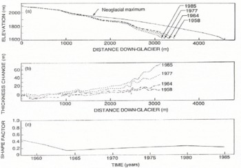
Fig. 2. Surface-elevation profiles for South Cascade Glacier (a), associated elevation changes for the length of the glacier above the 1985 terminus calculated relative to 1955 (b) and the corresponding profile-shape factor f(c). Data are from unpublished topographic maps made by the United States Geological Survey.
Morphological data
There is potentially an abundance of information about elevation-profile changes from Neoglacial to present based on elevation of moraine crests and trim lines in comparison to present glacier surfaces. We have chosen a small set of glaciers, listed in Table 1, for which data about moraines, terraces and other morphological features are easily available from detailed topographic maps. The choice of glaciers was also restricted to those with reasonably well-defined independent accumulation areas and heads. Many other mapped glaciers fitting these requirements could be added to the list. The list could be further expanded using field observations of trim lines and other data not discernible on topographic maps. Therefore, our list is in no way complete. Because of the geometric restrictions in our selection of glaciers, the list is not necessarily representative of all glaciers. However, we believe that it should be fairly representative of simple valley glaciers in the length range of a few to 10 km.
Table 1. Glacier data sets examined

The main difficulty for the morphological data is that elevation changes are not clearly defined in the upper parts of the glaciers where lateral moraines are usually absent. In fact, many glaciers with well-defined lateral moraines on maps were not used because their modern termini had retreated close to or beyond the highest map traces of the moraines. If usable data were not definable over more than the lowest one-quarter of the present length of a glacier, we did not include the glacier in our analysis. Table 2 gives the complete lengths and the lengths over which elevation changes were determined for the glaciers we selected. On many glaciers, any data about elevation changes in the accumulation area will be difficult to find by any means because of ice flow down the valley walls into the accumulation area. South Cascade Glacier provides one example where the elevation change from the Neoglacial maximum can be determined right up to the head of the glacier where lichen trim lines show that it is essentially zero (personal communication from M. F. Meier). Ground observations on others of the listed glaciers might similarly extend the length of usable data. In the absence of data in the upper parts of glaciers, we have extrapolated the available data for Δh headward as a linear variation between the highest data and zero at the head. This appears to be justifiable in most cases by analogy to South Cascade Glacier, especially when Δh at the highest data location is much smaller than near the terminus and there is a monotonie up-glacier convergence of the initial and final surfaces.
Table 2. Profile changes Neoglacial maximum to present

A second problem with regard to the morphological data concerns the relationship of identifiable moraine crests or trim lines with the former ice surface that produced them. The ablation areas of glaciers typically show convex-upward cross-profiles of surface elevation. The cross-profiles of the sampled glaciers are mostly that way now and were presumably so at their Neoglacial maxima but by unknown amounts. There may also be sideways tilts of the cross-profiles. To circumvent these difficulties partially, elevation change was estimated from the relative elevation of the moraine crest and the adjacent modern ice margin. When data from both sides of a glacier were available, these were averaged. In all cases, the current geometry was used as the reference geometry. This is advantageous because current lengths are shorter than in Neoglacial times.
A third problem arises because the lateral moraines and trim lines are probably time-transgressive (Reference NyeNye, 1990) and therefore do not represent any former surface at a definite time. This problem was neglected, which should not be serious because glaciers were close to their Neoglacial maxima for many decades.
Table 2 gives the values of the parameter f that were calculated by these methods. In view of the headward extrapolation of surface elevation used for most cases, it is not possible rigorously to establish an error estimate for the calculated f. Errors as large as 0.1 are possible, so values are tabulated only to the nearest 0.1 for those cases where extrapolation was necessary. The values for f fell in the range 0.1–0.4 with an average value equal to 0.28.
Reference WeidickWeidick (1968) also used morphological evidence to examine trends of thickness change Δh experienced by local glaciers in West Greenland during Neoglacial retreat. Instead of Δh versus x for individual glaciers, he tabulated Δh versus elevation for an ensemble of glaciers in a few regions. His results show that, between sea level and 1200 m, Δh decreases exponentially with a e-folding scale of about 430 m. Thickness change averaged over that elevation interval was about one-third of the sea-level value. In order to relate this result precisely to f as defined in this paper, it is necessary to know how the altitude range relates to the glacier lengths. In general, the local glaciers originate above 1200 m and the above average does not appear to include their upper reaches. As discussed below, the corresponding f value would be smaller than one-third. Although a precise comparison cannot be made with this information, the pattern in West Greenland glaciers appears to fall in the range for the mountain glaciers given in Table 2.
Geodetic data
In the European Alps, there are sequences of maps or surveying information that give data about elevation-change profiles over many decades on several glaciers. In recent decades, this data base has been expanded by the introduction of systematic observation programs in a number of countries. We have analyzed data from glaciers listed in Table 1.
These data are more accurate than the Neoglacial to present changes discussed above, since the elevation of the actual glacier surface at definite times is determined directly. Sequential map information is most easy to use because of completeness. However, some data were available only as surveyed profiles. The surveyed profiles sometimes did not include data close to the termini or heads of glaciers. In such cases, a reference head rh and reference terminus rt were chosen at the highest and lowest data locations. The parameter f was calculated over this sub-interval of the full glacier length. The range of f values calculated for all of the glaciers and time intervals examined (Table 1) were in the range 0.05–1.22. This wide range is not unexpected. Some of the data sets covered only part of the glacier length as discussed above. Most importantly, these data sets include both very short time-scale changes from one year to the next and multi-decade changes. The values calculated over short intervals include patterns of elevation change, where changes are not largest near the terminus (e.g. Unteraargletscher between 1929 and the mid-1930s, Kokanee Glacier between 1964 and 1972, and Nisqually Glacier between 1942 and 1973) or not of the same sign over the full length (e.g. Griesgletscher between 1961 and 1979). These patterns could be caused by transients in the response. A thorough analysis of these short time-scale phenomena has not been done, and we report results for the parameter ƒ determined for individual glaciers and time intervals only in those cases with multi-decade records spanning nearly the full glacier length (Table 3). Figure 3 shows results for thickness change versus distance in normalized form for those cases where data cover the full glacier length. The results for f fall in the range of the morphological data, Neoglacial to present, except for Unteraargletscher.

Fig. 3. Normalized thickness change versus normalized distance for multi-decade measurements covering the full glacier length.
Table 3. Profile changes measured by surveying and photogrammetry over multi-decade intervals

Discussion
Range of f
The results of our analysis show that, even for long time-scales, a unique characteristic value of f does not apply to all glaciers. This is not unexpected. Several potential causes for the spread in values may be identified.
Size of retreat. When the change in length of a glacier becomes a substantial fraction of the reference length, the usefulness of the concepts behind the profile-shape factor begin to break down. First of all, a large part of the total volume change will occur in the distance between the two termini. Furthermore, f is sensitive to the size of the change. For example, in theoretical models (e.g. Reference Jóhannesson, Raymond and WaddingtonJóhannesson and others, 1989b) for a retreated glacier, f goes from small values to large values near 1, as the fractional retreat goes from 0 to 1. This means that the values of f we observe for the sizable retreats from Neoglacial to present are biased upward in relation to values expected for infinitesimal changes. However, there is not a clear correlation between the size of retreat Δl/l and f evident in the data (Table 2), so other factors must also be important.
Longitudinal profile of bed slope. In a relative sense, glaciers are thin and fast where they are steep and thick and slow where they are less steep. Thickness changes should follow a similar pattern; such a pattern is clear in the data for elevation changes. One consequence is that glaciers which show steepening toward their heads will, other factors being equal, tend to have lower values of f. A very steep ice fall may also serve to decouple the dynamics of the parts of a glacier above and below it.
Longitudinal changes in bed cross-profile. A near-steady-state glacier must be relatively deep and/or fast where the cross-section shape constricts the width and relatively shallow and/or slow where the shape produces a large width. The variations of cross-profile along the length of a valley will therefore influence the surface profile of the ice. In particular, the shape variation will impose longitudinal variations in surface slope that may affect mass-balance-induced elevation-change patterns similar to those described above.
Global dynamics. Ice-motion processes exert a primary control on the longitudinal profile of a glacier. There will be a coupling between changes in thickness profile and any changes in ice dynamics such as the ice-deformation or sliding rates not directly related to stress (e.g. arising from thermal or hydrological effects). If sliding motion were turned off during a retreat, then the eventual steady state reached would have a steeper average surface slope and be thicker in its upper reaches than would be the case otherwise. This effect would tend to yield relatively less change in the upper reaches of a glacier and, therefore, lower f. Alternatively, if the ice were warmed and thus softened or sliding were enhanced during a retreat, these changes would yield a high f.
Terminus dynamics. Reference Jóhannesson, Raymond and WaddingtonJóhannesson and others (1989b) argued that f must be sensitive to the details of the terminus dynamics. More specifically, f describing the thickness change between two steady states should be proportional to the sliding velocity, u0 at the terminus (i.e. f ~ u0). Therefore, one may expect to see some differences depending on local basal conditions that promote or impede sliding at the terminus. Unfortunately, there are very few data to investigate this possibility. 588
We do not attempt to analyze all of the glaciers in terms of these effects, which would require knowledge of their ice-thickness distributions and extensive-flow modeling. However, we can, in some cases, see some consequences from longitudinal-slope variations.
Nisqually Glacier appears to provide one example. Its upper 4.7 km lie on the steep flanks of Mount Rainier, where the ice is presently thin and could not have been much thicker at the Neoglacial maximum. The lowest 2 km are less steep and significant thickness changes have occurred. This geometry must cause a relatively low value of f.
Rhonegletscher is another example. Between 1874 and 1915, there was substantial terminus retreat accompanied by major elevation changes below the ice fall but only minor changes above it (Reference MercantonMercanton, 1916). This pattern gave low values of f close to 0.1 even over short time intervals.
It would be particularly desirable to have an explanation for the high value of f found for Unteraargletscher, which appears to be anomalous in relation to the range of f found for the other glaciers. The terminus of the glacier was flooded in 1931 by the construction of a dam but the terminus had receded to emerge from the lake by 1961 (Reference HaefeliHaefeli, 1970). Since f is measured between times when the terminus was not affected by the lake, it seems unlikely that the effects from the lake are important. South Cascade Glacier also retreated through a (natural) terminal lake but it does not show any anomaly. Reference HaefeliHaefeli (1970) has suggested there was a large reduction in sliding rate with little change in internal deformation flow on Unteraargletscher during its retreat from its Neoglacial maximum. We would not be able to cite this as a cause of the anomalously high value of f, since that effect would tend to lower f. The extensive debris cover in the lower ablation zone could be a factor. However, we believe that the high value of f is in part caused by the length interval over which it was calculated. That length interval omits 4.4 km of the highest part of the glacier (Strahlegggletscher) near the head and 0.8 km of the lowest part near the terminus. If a linear extrapolation from the highest data to zero elevation change at the head is assumed, then the calculated value of f drops to 0.46. We expect that a significant further reduction in the calculated value of f would result from extending the calculation interval all of the way to the present terminus, in view of the rapid increase in thickness change toward the terminus found on other glaciers. Unfortunately, we do not know the surface elevation in 1929 at the present terminus position, so we cannot verify this explanation. Nevertheless, it is reasonable to suppose that the large value of f is a reflection of the spatial limitations of the available data and not necessarily indicative of anomalous dynamics or mass-balance history.
Above, we have emphasized the range of f and the possible causes. In view of the variety of processes that contribute to the value of f, we may be encouraged that the range is as small as it is. The mean value of about 0.3 that we have found is smaller than the value of 0.5 suggested as being typical in earlier literature (Reference NyeNye, 1960; Reference PatersonPaterson, 1981). Estimates for changes in volume and the response times of glaciers through Equations (2) and (3) will therefore be correspondingly smaller.
Volume change of glaciers
We may use the typical value of f to make a very rough estimate of the total volume change of glacial ice from the Neoglacial to present. We restrict attention to mountain glaciers and ice caps, where our phenomenological results could apply. We exclude the large ice sheets of Greenland and Antarctica, where changes at the margins over this time-scale (~102 years) may not be related to the full profiles because of their long memories.
From Equation (2), we estimate the volume change of a glacier above the modern terminus as fΔh(l0)a0, where do is the area above the terminus. We have found ƒ ~ 0.3, Δh(l0) ~ 0.1 km. These numbers estimate ΔV as ΔV = 0.03 km × a0 Obviously, this result cannot be used to get an accurate estimate of volume change on any specific glacier. However, we may regard it as a rough estimate typical of glaciers. The total volume change for all glaciers above their termini can then be found by summing their areas. The total area of glaciers and ice caps is about 5.4 × 10⁵ km2, which with the above numbers gives a total ΔV equal to 1.9 × 10⁴ km3. This volume, when spread over the area of the ocean (3.6 × 10⁸ km2), would have caused a sea-level rise of about 0.05 m occurring over a time-scale of 102 years at a mean rate of about 0.5 mm a−1. This mean rate of sea-level rise agrees well with 0.46 ± 0.26 mm a−1 estimated by Reference MeierMeier (1984) based on glacier mass-balance measurements.
The above estimate of total Neoglacial to present glacier-volume loss must be viewed with caution in view of the many assumptions. The formulation above does not include volume lost between the modern and Neoglacial termini. This additional volume loss may be written as ftΔh(l0)Δa where Δa is the area between the termini and ft is a factor which relates the mean thickness change over Δa to that at the modern terminus. The total volume change, including both contributions from above and below the modern terminus, is then

The second term in parentheses represents a correction from below the modern terminus. If the ice lost below the modern terminus is approximated as a wedge shape ft ~ 0.5, then ft/f ~ 1.6. For the smaller glaciers examined in Table 2, Δl/l and the corresponding Δa/a are sizable (up to 0.5), and the volume lost below the present terminus is definitely non-negligible. However, for the largest glaciers, Δl/l is close to 0.1 and the corresponding correction is about 20%. This value is probably smaller than uncertainties in f and Δh(l0), and other factors resulting from the simplified view of glacier geometry (e.g. width variations along the lengths). It is also questionable whether the phenomenology established on small-and intermediate-sized glaciers applies to the large glaciers of coastal Alaska and sub-polar ice caps that represent most of the ice area and probable contribution to sea-level change. Nevertheless, since our estimate is based on a completely different set of assumptions than Meier’s, the near agreement strengthens the case that melting of glaciers and ice caps has had a significant contribution to sea-level change.
Response time of glaciers
(Reference Jóhannesson, Raymond, Waddington and OerlemansJóhannesson and others 1989a, Reference Jóhannesson, Raymond and Waddingtonb) have derived an alternative estimate of the response time of a glacier described by

where h * is approximately the maximum thickness and bt is the (negative) mass balance at the terminus. Equations (3) and (4) are theoretically equivalent, but Equation (4) appears to give substantially shorter estimates of TM than does Equation (3) with f = 0.5 (Reference Jóhannesson, Raymond and WaddingtonJóhannesson and others, 1989b). Our examination of glacier-profile changes indicates the substantial quantitative difference between Equations (3) and (4) is not explained entirely by a grossly bad choice of f (0.5 instead of 0.3). Rather, the difference must arise partly from consistency of the values assumed for other quantities in the equations.
We examine a specific case for which all values are known from measurements (South Cascade Glacier in 1960) with l = 3.4 km, h = 200 m, bt = −6 m a−1, u(l) = 8 m a−1 (Reference Meier and TangbornMeier and Tangborn, 1965). Our results give f = 0.24. Equation (3) gives TM = 0.24 × (3400 m/ 8 ma−1) = 102 a. Equation (4) gives TM = (200 m/ 6 ma−1) = 33 a.
For order-of-magnitude analysis, these two estimates can perhaps be considered to agree. However, we can find a cause of the substantial difference by a factor of 3 in an inconsistency in the inputs to the equations: namely, the relative values of terminus velocity u(l) and ablation rate bt. In 1960, South Cascade Glacier was in rapid retreat. The terminus slope of South Cascade Glacier in 1960 was about tanα = 0.3 (Reference Meier and TangbornMeier and Tangborn, 1965). Thus, u(l) would have to be about-bt/tan α = 20 m a−1 for steady state with the actual balance rate. When this value of u(l) is put into Equation (3), TM is predicted to be 41 a, in good agreement with the prediction of Equation (4). Alternatively, one could suppose that –òt would have to be u(l) tanα = 2.4 m a−1 for steady state with the actual velocity. This value in Equation (4) gives TM equal to 83 a, in good agreement with Equation (3). From this point of view, Equations (3) and (4) are numerically consistent. The inconsistency arises between the measured u(l) and bt because the terminus is far out of steady state.
Refinement of an estimate for TM hinges on whether to use the actual velocity or the actual balance rate. We suggest this question illustrates a fuzzy nature to the estimate of TM for a glacier distinctly out of steady state or, in the terms of Reference NyeNye (1960), far from a datum state that can actually be achieved. South Cascade Glacier will retreat up-valley to reach an eventual steady state where the terminus balance rate is less negative and the terminus velocity is higher, and they are related to one another in a consistent way compatible with steady state for the terminus slope. The asymptotic approach to this final steady state will be controled by a TM given by either Equation (3) or (4) governed by consistent f, u(l) and bt that are different from those that exist at present.
Conclusions
Our principal conclusions may be listed as follows:
Retreat of glaciers from Neoglacial maxima has caused thickness changes that decrease headward from the terminus.
In almost all cases, the thickness change decreases more strongly than linearly with distance.
The shape of the longitudinal profde of thickness change is typically described by a profde factor f in the range 0.1–0.4, with 0.28 being an average value. This range may be compared with a profile factor of 0.50 which corresponds to a variation of thickness change that is linear with longitudinal distance.
Application of the profile factors to estimate total volume change of glaciers and ice caps from Neoglacial to present supports the view that their melting has had a significant contribution to observed sea-level rise.
Dissimilar estimates of the memory length of glaciers based on length l divided by velocity u (Equation (3)) compared to thickness h divided by terminus ablation rate bt (Equation (4)) are not entirely resolved by the difference in profile factor f of ~0.3 found in this study and f of ~0.5 earlier assumed as characteristic. An important contribution to the discrepancy may be inconsistency among measured velocity, ablation rate and slope when the terminus is distinctly out of steady state.
Profile-shape factors for thickness changes measured over short intervals of a few decades or less show a much wider range than exists for long time-scale changes.
The difference in range for profile-shape factors for short time-scale changes compared to long time-scale changes illustrates the theoretical separation into a short time-scale response where transients may cause complex localized thickness-change patterns and a long time-scale response displaying changes in near-steady-state profiles controled by more global dynamics.
Acknowledgements
We wish to thank A. Flotron and R. Krimmel, who provided unpublished data. A. Iken, M. Aellen and J. Schweizer gave valuable assistance while gathering data sources in Switzerland. Publications of the World Glacier Monitoring Service were especially useful in the research. Comments from T. Jóhannesson, Ε. Waddington, Ν. Reeh and an anonymous reviewer contributed to improvements in the final manuscript. This work was supported by grant number EAR 8708391 from the U.S. National Science Foundation.
The accuracy of references in the text and in this list is the responsibility of the authors, to whom queries should be addressed.


