


Introduction
The experimental study of englacial and subglacial hydrological systems is inherently challenging due to the difficulty of accessing such systems. Various field techniques have been applied, including (1) water-level measurements, as a proxy for subglacial water pressure, in boreholes (e.g. Fountain, Reference Fountain1994; Hubbard and others, Reference Hubbard, Sharp, Willis, Nielsen and Smart1995; Harper and others, Reference Harper, Humphrey and Greenwood2002) and moulins (e.g. Iken, Reference Iken1972; Andrews and others, Reference Andrews2014; Covington and others, Reference Covington, Gulley, Trunz, Mejia and Gadd2020), (2) tracer experiments between multiple boreholes, moulins or the glacier outlet to infer, for instance, discharges, transit velocities and dispersion coefficients (e.g. Sharp and others, Reference Sharp1993; Nienow and others, Reference Nienow, Sharp and Willis1998; Hock and others, Reference Hock, Iken and Wangler1999; Schuler and others, Reference Schuler, Fischer and Gudmundsson2004; Cowton and others, Reference Cowton2013), (3) direct exploration of moulins (e.g. Holmlund, Reference Holmlund1988; Gulley and others, Reference Gulley2014; Mankoff and others, Reference Mankoff2017) and (4) imaging through borehole cameras, to determine the structure of englacial drainage systems (e.g. Fountain and others, Reference Fountain, Jacobel, Schlichting and Jansson2005; Church and others, Reference Church2019). Current developments include measurement techniques such as the Cryoegg (Prior-Jones and others, Reference Prior-Jones2021), the Glacsweb wireless probe (Hart and others, Reference Hart2019) or drifters (Alexander and others, Reference Alexander2020) that can be deployed into glacier streams to take in situ measurements. In addition to these in situ measurement techniques, remote geophysical methods have been used to infer properties of glacier drainage systems by radar and seismic imaging (e.g. Harper and others, Reference Harper, Bradford, Humphrey and Meierbachtol2010; Schroeder and others, Reference Schroeder, Blankenship and Young2013; Church and others, Reference Church2019, Reference Church, Bauder, Grab and Maurer2021; Egli and others, Reference Egli, Irving and Lane2021) or by passively measuring seismic noise (e.g. Dalban Canassy and others, Reference Dalban Canassy, Röösli and Walter2016; Gimbert and others, Reference Gimbert, Tsai, Amundson, Bartholomaus and Walter2016; Röösli and others, Reference Röösli, Walter, Ampuero and Kissling2016; Nanni and others, Reference Nanni2020).
However, with the current understanding of englacial and subglacial drainage systems, physical models that aim at representing these systems still require a number of assumptions and involve poorly constrained model parameters, which motivates field experiments such as the one presented in this study. The validation of such models is difficult since measurements of subglacial water pressure, temperature, discharge and flow speed are usually sparse in space and time. Moreover, these measurements often represent bulk values over large portions of the glacier (e.g. Werder and others, Reference Werder, Schuler and Funk2010). Irarrazaval and others (Reference Irarrazaval, Werder, Huss, Herman and Mariethoz2021) used one of the most comprehensive sets of observations of a glacier drainage system (Huss and others, Reference Huss, Bauder, Werder, Funk and Hock2007) to invert a subglacial drainage model for channel locations and discharge conditions. They found that the available data are insufficient to uniquely constrain the model parameters and that more frequent observations at higher resolution are needed for appropriate constraint. Brinkerhoff and others (Reference Brinkerhoff, Aschwanden and Fahnestock2021) arrived at largely the same conclusion as they coupled a subglacial drainage model (Werder and others, Reference Werder, Hewitt, Schoof and Flowers2013) to an ice dynamics model thus enabling the use of surface velocity measurements to invert for subglacial drainage properties.
An example for the lack of experimental model validation is the concept of R-channels (Röthlisberger, Reference Röthlisberger1972), (semi)circular, ice-incised, pressurised conduits that are opened by melt and closed by viscous ice deformation. For such features, melt is commonly calculated under the assumption that the water temperature follows the pressure melting point and that the frictional and sensible heat results in instantaneous melting of the ice walls. Since their first mathematical description in Röthlisberger (Reference Röthlisberger1972), R-channels have been incorporated into the majority of subglacial drainage models to represent the efficient drainage system (e.g. Flowers, Reference Flowers2015; De Fleurian and others, Reference De Fleurian2018). However, even after decades of applying the theory, the aforementioned assumptions are yet to be validated and the parameters still need better constraints. The latter is particularly important in terms of the friction factor, which controls frictional energy loss and thus the energy available for melting the surrounding ice by parameterising the hydraulic roughness of the channel.
In this paper, we present a new approach to experimentally assess the properties of an englacial R-channel. By using boreholes connected to the subglacial drainage system and supplying them with water from a glacier surface stream, we create englacial features that route the water from the surface to the glacier bed; we use the term artificial moulin to refer to such a feature. The part of an artificial moulin which is below the water level experiences pressurised water flow and is thus an artificial, englacial R-channel, which is the focus of this study. Although the concept of artificial moulins as a field technique is not completely new, it has only been used for piezometric observations of the water level (e.g. Röthlisberger and others, Reference Röthlisberger, Iken and Spring1979). Here, we combine pressure and temperature measurements with salt dilution gauging to derive the temporal evolution of the channel's hydraulic gradient, discharge, water flow speed and cross-sectional area. This way we are able to examine the hydraulic and thermodynamic properties of a single R-channel in detail. The highly resolved time series of both the hydraulic friction factor and of the cross-sectional area enable us to directly test the basic theory of Röthlisberger (Reference Röthlisberger1972). In contrast to a natural moulin with its complex geometry, an artificial moulin enables safe deployment of instruments and thus precise measurements, which in turn allows the calculation of R-channel properties.
Methods
Field site
We conducted our experiment in August 2020 on Rhonegletscher, a valley glacier in the central Swiss Alps covering an area of ~15 km2 (as of 2019), elevations from 3600 to 2200 m a.s.l. and a length of ~8 km (GLAMOS, 1881–2020). The study site was located in the ablation zone between 2450 and 2500 m a.s.l. where a bedrock overdeepening is present. There the ice is ~200 m thick (Grab and others, Reference Grab2021) and the ice surface slope is 5° southwards (Fig. 1). In summer, local daily ice melt reaches 0.1 m d−1, supplying meltwater to surface streams (Landmann and others, Reference Landmann2021). The streams relevant for our study site originate from several smaller streams ~700 m up-glacier. When crossing the region of the overdeepening, the streams merge into a few larger ones, with discharges of several hundred litres per second each (Fig. S1). In this region, ice flow is compressional and only a few small surface crevasses are present. Just downstream of the study site, these surface streams enter the glacier via moulins (Fig. 1).

Fig. 1. (a) Location of Rhonegletscher (blue dot) within the borders of Switzerland (black); (b) outline of Rhonegletscher (blue) and indication of study site (black rectangle); (c) map of the study site indicated in (b), including positions of all boreholes and artificial/natural moulins, the closest surface streams, surface and bed topography as well as the glacier outline. The glacier outline in (b) and (c) refers to the state 2016 (Linsbauer and others, Reference Linsbauer2021). Coordinates are given in the CH1903+/LV95 coordinate system. Figure S1 provides an aerial image of the site.
Artificial moulins
We created artificial moulins by drilling boreholes of ~0.1 m diameter with a hot water drill (Iken and others, Reference Iken, Röthlisberger and Hutter1976). The boreholes were placed next to relatively large surface streams and were drilled down to the glacier bed. Boreholes which drained were interpreted as to have connected to the glacier's efficient drainage system and were turned into artificial moulins by diverting the neighbouring surface stream into them. Only one (BH15, Fig. 1) of the five drilled boreholes (BH11–BH15) drained directly after the drill reached the bed. The artificial moulin created from this borehole, named AM15, was used for the experiment during the following two weeks. Meanwhile, we kept monitoring the water level in the other boreholes and eventually turned the one with the largest diurnal water level fluctuations (BH13) into an additional artificial moulin (named AM13).
BH15 was drilled on 7 August 2020 to a depth of 187 m and turned into an artificial moulin on 8 August. For the first two days of the experiment (8 and 9 August) the flow in AM15 was pressurised, indicated by a completely water-filled borehole. During the following days, however, the water level dropped continuously. The limiting factor for supply of water to AM15 was the incision rate of the surface stream's spillway to the moulin. Only about half of the stream's water entered AM15. As our experiment relies on pressurised flow, we tried to maximise the water supply through frequent enlargement of the spillway with a pickaxe. However, starting from 10 August it was not possible anymore to maintain pressurised flow with this method.
BH13 was drilled on 6 August 2020, reaching the bed at a depth of 200 m. While there was no direct drainage, 20 h later the water level had dropped by 42 m. On 20 August, we diverted a stream into it (turning it into AM13, Fig. 2a) but measurable flow was only established during the following night. AM13 was completely water-filled for the entire duration of the experiment between 20 and 21 August.
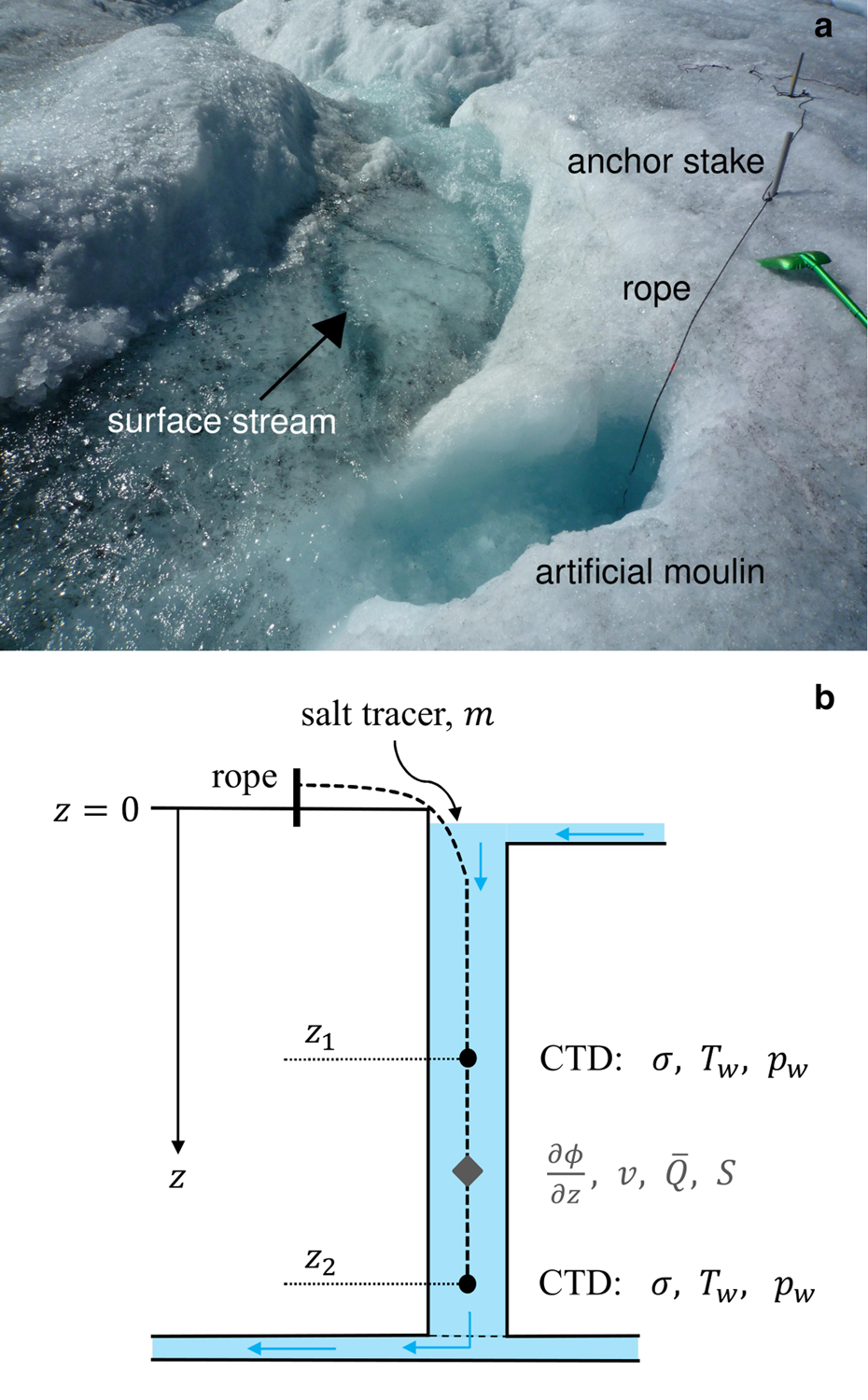
Fig. 2. (a) Artificial moulin AM13 (diameter ~0.2 m) and the feeding surface stream. The rope carrying the conductivity-temperature-pressure sensors (CTDs) is attached to stakes drilled into the ice. The green shovel on the right side of the picture is ~1 m long, for a measure of scale. (b) Schematic setup of the experiment. Two CTDs are installed at two different depths, z 1 and z 2, which span a test-section of varying length (between 30 and 100 m, see Table S1) and measure conductivity σ, water temperature T w and water pressure p w. We use these measurements to derive the hydraulic gradient ∂ϕ/∂z, flow speed v, mean discharge $\bar Q$ and cross-sectional area S as averages over the test-section.
Instrumentation
The instrumentation in each artificial moulin consisted of two Keller DCX-22-CTD loggers measuring electrical conductivity, temperature and pressure. We refer to these loggers as CTDs. The instrumental uncertainty of conductivity was ±5 μS cm−1 (microsiemens per centimetre) and the one of temperature ± 0.05 °C. The pressure sensors of the two loggers measured with an uncertainty of ±490 and ±1470 Pa, proportional to their full scale range of up to 100 and 300 m water head, respecively. Each day, we attached the two CTDs at different positions on a static rope and installed them in the artificial moulin such that the lower sensor, which was attached to the end of the rope, was located at least 10 m above the glacier bed, i.e. at ~170 m depth for AM15 and at ~190 m depth for AM13. Once installed, we did not change the setup during one day of measurements. The weight of the sensors and the downward water flow ensured that the sensors’ positions were stable. The general setup is shown in Figure 2b and a list of the sensor depths on individual days in the Supplementary material (Table S1). We always used the same two loggers and never changed their relative position.
The rope itself served as a depth and sensor distance measure. Its length was measured under tension typical of that experienced during deployments and we estimate the uncertainty of the sensor distance to be ±1 m. The sensors were lowered by hand into the artificial moulin in the morning and retrieved in the evening on a daily basis, which was necessary to download the recorded data and reset the loggers for the next day. We used a 1 s sampling interval to allow for ~8 h of recording time per deployment.
Our individual tracer experiments characterise the section of the artificial moulin between the two sensors. We call this section the test-section. Under the constraint that both sensors had to be submerged, the length of this section was chosen as large as possible (up to 100 m) in order to minimise uncertainties per unit length. This constraint was the reason to reduce the length of the test-section in AM15: six days after activation (14 August), the water level had dropped to 130 m below the surface at mid-day, when the water supply reaches its daily maximum. As a consequence, the upper sensor (at 127 m depth) was left out of the water during the entire day. Eleven days after activation (19 August) the flow was only pressurised to less than 20 m above the lower sensor.
Experimental setup
In this study, artificial moulins represent pressurised englacial R-channels rather than moulins themselves. To investigate the properties of such an R-channel, we use the pressure and depth measurements to infer the hydraulic potential gradient and salt tracer experiments to obtain the discharge and the flow speed. Using these quantities we derive the rest of the hydraulic properties as listed in Table 1.
Table 1. Quantities measured and derived through the experiment. The two uncertainties for the water pressure correspond to the upper and lower CTD sensor, respectively.

Water flow in an R-channel (and in general) is driven by the gradient of the hydraulic potential, or hydraulic gradient for short. Neglecting the kinetic potential, the hydraulic potential is given by the sum of elevation potential and water pressure

where ρ w is the density of water, g the gravitational acceleration, h the elevation relative to a reference point and p w the water pressure. We neglect the kinetic potential as it is commonly done in glaciology (e.g. Röthlisberger, Reference Röthlisberger1972) and since its gradient is more than an order of magnitude smaller than that of the other components (see Supplementary material). A summary of all physical constants used in this study is given in Table 2 and the symbols and units for physical quantities are listed in Table 1. In our experiment, measuring water pressures at the two sensors with known depths enables us to calculate the hydraulic gradient along the flow direction of the test-section. Since we constructed the experiment to produce purely vertical flow, we can write the hydraulic gradient as

where z is the depth coordinate pointing downwards (in our case along flow), Δp w the pressure difference and ℓ the length of the test-section. When deriving other quantities from the so-computed hydraulic gradient, we use the pressure averaged over a time period which starts when the tracer is first visible in the readings of the upper sensors and ends when it ceases to be visible in the readings of the lower sensor. This duration is mostly ~2–3 min in AM15 and between 20 and 30 min in AM13 where the velocities and discharges are smaller and the test-section is longer.
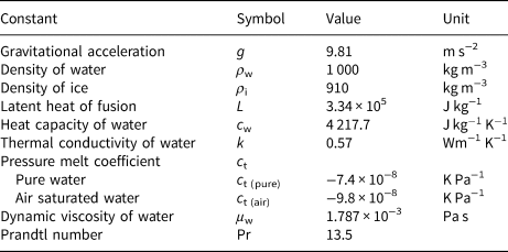
Table 2. Physical constants used for deriving relevant quantities (listed in Table 1, Eqns (1–8)), running the size evolution models (Eqns (9) and (10)) and calculating the heat transfer parameters (Eqns (11–16))
The discharge and the water flow speed are obtained by salt dilution gauging using measurements of electrical conductivity. In the field, we performed discrete injections of NaCl with a known mass, typically 25–100 g, at time intervals spanning from 20 min to a few hours. The mass was measured with an analogue suspended scale, and we estimated the uncertainty to 2 g by repeated comparisons with a digital kitchen scale. Before injecting the salt, we dissolved it in ~1 L of water. For a well-mixed salt tracer in a confined channel, the injection mass m is equal to the time integral of discharge Q times the salt concentration c. Assuming that the discharge is constant over the course of a tracer signal, one can write

with the integration interval [t 0, t 1] over the time span during which the concentration is above the background level. The salt concentration c(t) is proportional to electrical conductivity σ(t), and the factor of proportionality is determined from four calibrations conducted in the field. In each calibration, we measured the conductivity at different known salt concentrations, which is used to fit a linear function c = a σ with a proportionality factor a for each sensor. The time series of c(t) in the individual tracer experiments further allow the calculation of the average flow speed v, for which we use

with $\Delta t_{c_{\max }}$ being the time difference between the peak concentrations at the two sensors. Finally, the test-section's average cross-sectional area S is obtained with

where $\overline {Q}$ is the mean value between the discharges at the two sensors. Note that we only conduct this calculation when the discharges at the two sensors agree within their uncertainties. Finally, the Reynolds number, a measure of turbulence, is given by

with μ w being the dynamic viscosity of water.
Propagation of uncertainties
For the forward propagation of measurement uncertainties we use a Monte Carlo approach: quantities with uncertainties are represented with ensembles of 20 000 samples each from Gaussian distributions with standard deviations equal to the given or estimated uncertainties (Table 1). All calculations are then carried out with these ensembles, in turn yielding ensembles of results with the corresponding statistical distributions. These Monte Carlo uncertainty calculations are carried out using the software package MonteCarloMeasurements.jl (Bagge Carlson, Reference Bagge Carlson2020). Note that we treat the stated instrumental uncertainties (Table 1) as systematic and thus the mean of repeated measurements does not have a reduced uncertainty. The uncertainties of the derived quantities are stated as the standard deviations of the resulting distributions and are plotted with error bars in Figures 3–5.
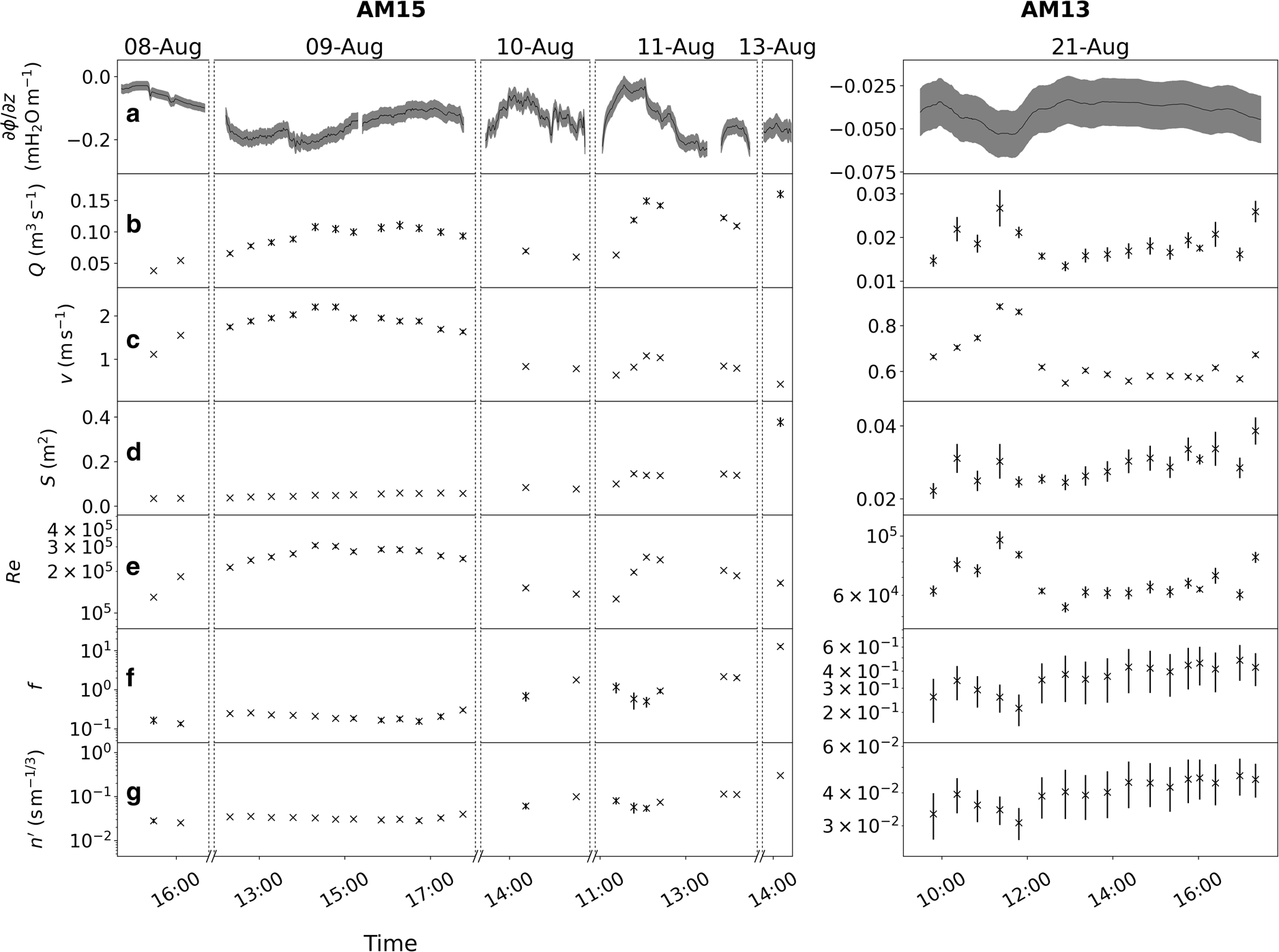
Fig. 3. Quantities derived for the test-section of the investigated artificial moulins (AM) (corresponding to Eqns (2–8)). The following quantities are shown: (a) hydraulic gradient ∂ϕ/∂z, smoothed with a moving average filter with window of size ±1 min (AM15) and ±15 min (AM13), which is the typical duration during which the tracer is visible; (b) discharge Q; (c) flow speed v; (d) cross-sectional area S; (e) Reynolds number Re; (f) Darcy–Weisbach friction factor f and (g) Manning roughness n′. Note that the scale of the y-axis differs between AM15 (left) and AM13 (right) and that measurements of the hydraulic gradient are logged continuously while the other quantities rely on manual tracer injections. For the hydraulic gradient, we only show measurements where the flow between the two sensors is pressurised. Uncertainties are given as one standard deviation and are represented by either a grey area (hydraulic gradient) or vertical lines (other quantities).
Friction factor
Discharge and flow speed are related to the hydraulic gradient, which is commonly captured in terms of the empirical Darcy–Weisbach equation (Weisbach, Reference Weisbach1845). In the case of a circular, vertical conduit it reads

where f is the Darcy–Weisbach friction factor, which can be understood as an effective factor absorbing any effects of non-circular conduits. However, in our setup we do not expect major deviations from the circular cross-section since the conduits of interest are both pressurised and vertical, which prevents local incision, and since we conducted the experiment within one week after drilling, a timescale where viscous ice deformation should be of minor importance. Since we measure and derive all remaining quantities, we can compute f directly. To do so, we use the spatial discretisation from Eqn (2) for ∂ϕ/∂z and take $\overline {Q}$ for the discharge. Thus the derived friction factor is also an average value over the test-section. The calculation of f through Eqn (7) is only applicable when the flow is pressurised rather than a waterfall.
In order to facilitate comparisons with other studies, we also compute the Manning roughness n′, which is often used as an alternative way to relate the hydraulic potential to discharge. For a circular channel, the conversion between f and n′ is (e.g. Clarke, Reference Clarke2003)

Model for channel size evolution
According to Röthlisberger (Reference Röthlisberger1972), R-channels are opened through melting the ice walls. In Röthlisberger's formulation, the amount of melt is obtained from considerations of energy balance, where the energy for melt is provided both by frictional dissipation and by sensible heat changes due to the water temperature changing along the channel. In the majority of subglacial drainage models, the temperature is assumed to be at a constant offset from the pressure-dependent melting point (Flowers, Reference Flowers2015). Under this assumption, the temperature gradient is equal to the gradient of the pressure melting point and obtained directly from multiplying the pressure gradient with the pressure melt coefficient c t. The fact that this approach avoids solving for the water temperature as a field variable makes it numerically cheap and attractive to apply.
In order to test this assumption, we simulate the size evolution of our test-sections with two different models. In the simpler one, we follow the aforementioned assumption, therefore fixing the temperature gradient at the melting point gradient (referred to as the c t-gradient model), and in the second model we perform a Bayesian inversion with the temperature gradient as a parameter that we fit to the experimental data of the cross-sectional area (the free-gradient model). The latter allows us to determine a confidence interval for the temperature gradient, and we can test whether the temperature gradients predicted by the c t-gradient model are included within that interval. In both models, we neglect the closure of R-channels through viscous ice deformation since it is insignificant in our case: after calculation it turns out that the largest closure rates are three orders of magnitude smaller than the opening rates (Table S3, Figs S3 and S4).
In the c t-gradient model, the evolution of the cross-sectional area is described through

where ρ i is the ice density, L the latent heat of fusion and c w the heat capacity of water. The first term, proportional to ∂ϕ/∂z, describes frictional heat dissipation while the second one, proportional to the melting point gradient c t∂p w/∂z, is related to the sensible heat. Here, we take c t as negative, noting that it is also common to define it as positive (e.g. Clarke, Reference Clarke2003). Since c t depends on the air saturation of the water, its value is not accurately constrained. Two values are typically used: for pure water c t (pure) = −7.4 × 10⁻⁸ K Pa−1 and for air saturated water c t (air) = −9.8 × 10⁻⁸ K Pa−1 (Harrison, Reference Harrison1975). We forward-propagate uncertainties through the c t-gradient model by assuming that the c t values are uniformly distributed over the interval [c t (air), c t (pure)] and by using the above-determined uncertainties for Q, ∂ϕ/∂z, ∂p w/∂z and the initial S. Both models predict the evolution of S over the time period of tracer experiments on a single day, therefore the initial condition describes the state when the first tracer was injected on the corresponding day.
For the free-gradient model, we replace the melting point gradient in Eqn (9) by a general temperature gradient

where T w is the water temperature. Note that more negative water temperature gradients lead to larger opening rates. We fit the evolution of S modelled through Eqn (10) to the experimental data of S by a Bayesian inversion (Bayes, Reference Bayes1958) using ∂T w/∂z and the initial S as the fitting parameters. For the likelihood function, which compares modelled and measured S, we impose a Gaussian distribution on the uncertainties. This is done by assuming independent measurements and by using the measurement uncertainty as the distribution's standard deviation. As a prior for the initial S, we choose a Gaussian distribution around the measurement with its uncertainty as standard deviation. For the prior of ∂T w/∂z, we impose a uniform distribution which is non-zero only for ∂T w/∂z ∈ [−10−2, −10−6] K m−1. (See the Supplementary material, in particular Eqns (S7–S8), for a detailed description of the mentioned priors and likelihoods.) Uncertainties of the input parameters $\overline {Q}$ and Δp w/ℓ are neglected as otherwise the number of fitting parameters would increase from 2 to ~30. We run the Bayesian inversion by employing an affine invariant Markov chain Monte Carlo (MCMC) sampler (Goodman and Weare, Reference Goodman and Weare2010) with 106 iterations via the software package KissMCMC.jl (Werder, Reference Werder2021). To discretise the spatial derivative in Eqns (9) and (10), we use Eqn (2). For the time stepping we use an explicit forward Euler scheme with the time step equal to the interval between tracer injections (i.e. ~20 min).
Heat transfer
When water flows in a long R-channel under steady conditions, the water temperature approaches an equilibrium temperature T eq (Isenko and others, Reference Isenko, Naruse and Mavlyudov2005; Sommers and Rajaram, Reference Sommers and Rajaram2020). In our case, where the channel is vertical and pressurised, T eq changes along the flow due to the depression of the pressure melting point. Here, it is rather the offset of T eq from the melting point that approaches an equilibrium. In the following, we refer to this offset as the offset-temperature τ = T − T i, where T i is the ice temperature. Note that T can either refer to the water temperature T w or to the equilibrium temperature T eq with corresponding offset-temperatures τ w and τ eq, respectively. The ice temperature T i is assumed to be at the pressure melting point since Rhonegletscher is a temperate glacier.
From the steady-state energy balance along the channel, a water temperature equation can be derived (Eqns (S10–S16)). When stated in terms of the offset-temperatures, it reads

where

and z eq the equilibrating length scale

Here, k is the thermal conductivity of water and $\hbox {Nu}$ the Nusselt number quantifying turbulent heat transfer. Solving Eqn (11) gives

where τ w0 is the water offset-temperature at z = 0.
If we know$\hbox { Nu}$ , we can gain insights into the thermodynamics of the system by using both our measurements and the free-gradient model outputs to derive the thermodynamic variables z eq, τ eq and τ w. In particular, the free-gradient model allows us to constrain the temperature gradient ∂T w/∂z more accurately than the measurements, thus we use ∂τw/∂z = ∂T w/∂z − c t∂p w/∂z. The Nusselt number$\hbox {Nu}$
 is not accurately constrained but can be obtained from hydraulic variables via empirical formulas. Most commonly used is the Dittus–Boelter equation

where ${\rm {Pr}} = 13.5$ is the Prandtl number and $\hbox { {Re}}$
 is given by Eqn (6). Another formula to obtain Nu is the Gnielinski correlation (Gnielinski, Reference Gnielinski1975)

which additionally depends on the hydraulic friction factor f. To obtain the thermodynamic variables described above, we calculate Nu with six different parameterisations, summarised in Table 3. Five of them correspond to different sets of coefficients for the Dittus–Boelter equation (Eqn (15)) and the sixth parameterisation is the Gnielinski correlation (Eqn (16)). The parameterisation of Nu depends on the flow regime and thus the different correlations are always associated with certain ranges of Re values, which are also given in Table 3.
Table 3. Parameterisations used to calculate $\hbox { Nu}$ and the range of Re values for which they were determined. For the ones based on the Dittus–Boelter equation (Eqn (15)), dimensionless coefficients A, α and β are given. The different parameterisations are categorised into low and high heat-transfer, corresponding to low and high Nu values, respectively, for the conditions encountered in this study.
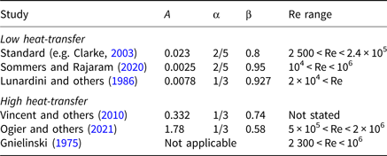
First, we use a set of coefficients that has been the standard in glaciology (e.g. Nye, Reference Nye1976; Spring and Hutter, Reference Spring and Hutter1982; Clarke, Reference Clarke2003) even though they were derived for engineering applications with experiments of water flowing through heated pipes. The coefficients of Lunardini and others (Reference Lunardini, Zisson and Yen1986) were also obtained from laboratory experiments but specifically in an ice-water related setup. In recent years, the Dittus–Boelter coefficients were fitted to glaciological field data (Vincent and others, Reference Vincent, Auclair and Meur2010; Ogier and others, Reference Ogier2021), albeit for surface streams with relatively warm water coming from a lake. Furthermore, we apply a set of coefficients that was proposed by the theoretical study of Sommers and Rajaram (Reference Sommers and Rajaram2020) for the case where all heat is generated by frictional dissipation. Finally, we apply the Gnielinski correlation, which is a refinement of the Dittus–Boelter equation with standard coefficients but which has had limited application in glaciology to date (Ancey and others, Reference Ancey2019). For each of these Nu parameterisations, we calculate τ w using Eqn (11) and compare it to our temperature measurements in order to test whether the different parameterisations for$\hbox { Nu}$ are applicable to our test-section.
Results
Measurements
In the time period 8–21 August 2020, we performed a total of 70 tracer injections in the two artificial moulins AM15 and AM13. After calculation of the discharge, we select 40 tracer experiments suitable for further considerations. The selection is based on two criteria: we require that (1) both sensors are at least 5 m below the water table, recognisable from the pressure record and (2) the discharge estimates at the two sensors are consistent, i.e. overlapping within their uncertainty ranges. In AM15, which we used for the experiment from 8 to 19 August, the limiting factor is the continuously dropping water level (see Fig. S2 and ‘Data/code availability’ section). In AM13, where the experiment lasted only for two days (20 and 21 August), the selection of only the second day is due to insufficient water flow on the first day.
Selected measured and derived quantities are summarised in Figure 3 (see also Table 1). In AM15 (left panels), discharge and flow speed measurements of 9 and 11 August capture daily variations, with peak values in the early afternoon. The flow speed decreases over the six day measurement period, whereas the discharge and the hydraulic gradient do not show a recognisable trend. Consequently, the cross-sectional area increases over time, with a clear linear trend on 9 August. Note that the inflow into AM15, and therefore the melt enlargement, was stopped during the nights from 8 to 9 and 9 to 10 August. In AM13 (right panels of Fig. 3), the absolute hydraulic gradient is low throughout the single day of measurements. Accordingly, the discharges, velocities and the opening rate of the cross-sectional area are much smaller than in AM15. The friction factor f fluctuates between 0.1 and 0.4 on 8, 9 August (AM15) and 21 August (AM13), corresponding to n′ between 0.02 and 0.04 s m−1/3. In AM15, the friction increases from 10 August onwards to reach a maximum of f = 13 on 13 August.
Observed and modelled size evolution
To compare the modelled opening rates to the measurements, we focus on the two days with the most dense measurements, i.e. 9 and 21 August 2020 (using AM15 and AM13, respectively); we will refer to them as 9-Aug/AM15 and 21-Aug/AM13, respectively. On both days, the size evolution inferred from the c t-gradient model overlaps with the measurements (Fig. 4) meaning that the c t-gradient model is in principle successful at predicting the evolution of the cross-sectional area. However, the prediction of the free-gradient model follows the measurements more accurately.

Fig. 4. Size evolution of the cross-sectional area S of artificial moulin (a) AM15 on 9 August 2020 and (b) AM13 on 21 August 2020 as calculated from measurements (black markers with error bars), the c t-gradient model (blue area) and the free-gradient model (grey lines resulting from some of the individual MCMC iterations fitting ∂T w/∂z and the initial S). The lower panels show probability densities for the temperature gradient for 9-Aug/AM15 (c) and 21-Aug/AM13 (d): temporal mean of measured temperature gradient $\overline {\Delta T_{\rm w}}/\ell$ (black line); temporal mean of melting point gradient as predicted by the c t-gradient model (blue); posterior distribution of ∂T w/∂z inferred by the free-gradient model (grey) with 95% confidence interval (CI) highlighted explicitly (dark grey).
Figures 4c, d show the temperature gradients corresponding to the c t-gradient model, the free-gradient model and the measurements. We compare the posterior distribution of ∂T w/∂z of the free-gradient model to the temperature gradient distributions both calculated from temperature measurements and predicted by the c t-gradient model. The observed temperature gradients agree with both models’ results, but the measurement uncertainties are too large to make any further statements about the question whether the temperature gradient follows the depression of the pressure melting point. For 9-Aug/AM15, the uncertainty is notably larger since the length of the test-section ℓ is only 50.6 m (compared to 101.5 m for 21-Aug/AM13). With a test-section of ~100 m, achieving an observational accuracy comparable to the model results would require measurement uncertainties of absolute temperature smaller than ~0.002 °C.
The temperature gradient of the c t-gradient model (the melting point gradient) overlaps with the 95% confidence interval of the posterior from the free-gradient model inversions on both days, meaning that the c t-gradient model is able to explain the derived S time series for each day individually. However, the overlaps are only small and on opposite ends of the c t range for the two days: for 9-Aug/AM15, only the models with c t values close to the lower limit c t (pure) (smaller absolute gradient) lie within the confidence interval, whereas for 21-Aug/AM13 only the values close to the upper limit at c t (air) lie therein. Since there is no indication for the c t values being different between the two days, it follows that the c t-gradient model is not able to explain the time series of both days simultaneously. This means that the actual water temperature gradients are different from the ones predicted by the c t-gradient model.
The models can also be used to calculate the relative contributions of frictional dissipation and sensible heat change to ice melt. The c t-gradient model predicts that averaged over the day, sensible heat provides $66\pm 7\percnt$ of the total energy for 9-Aug/AM15 and $90\pm 11\percnt$
 for 21-Aug/AM13, when the discharges and hydraulic gradients are smaller. In the free-gradient model, the contribution of sensible heat is $57\pm 4\percnt$
 for 9-Aug/AM15 (smaller than in the c t-gradient model) and $94\pm 6\percnt$
 for 21-Aug/AM13 (larger than in the c t-gradient model). Compared to the free-gradient model, the c t-gradient model predicts total melt rates that are on average $26\pm 9\percnt$
 larger for 9-Aug/AM15 and $40\pm 6\percnt$
 smaller for 21-Aug/AM13. The opening rates of both models and their partitioning are plotted and listed in the Supplementary material (Fig. S3, Table S3).
Heat transfer
Since the heat transfer calculations depend on the results from the size evolution models, we focus on the same days here, 9 August (AM15) and 21 August 2020 (AM13). Figure 5 shows the daily mean values for the thermodynamic variables z eq, τ eq and τ w, as well as τ w − τ eq for the different Nusselt number parameterisations. Note that we treat the different coefficients for the Dittus–Boelter equation as individual parameterisations.

Fig. 5. Daily means of thermodynamic properties, derived from six different ${\rm {Nu}}$ parameterisations (Eqns (15) and (16), Table 3): (a) Nusselt number $\hbox {Nu}$
 , (b) equilibrating length scale z eq, (c) equilibrium offset-temperature τ eq, (d) water offset-temperature τ w and (e) difference between water offset-temperature and equilibrium offset-temperature. Panel (d) also shows the 95% confidence interval of the τ w measurements. The figure only shows daily mean values because the daily variations are much smaller than the difference between the daily mean values of the $\hbox {Nu}$
 parameterisations (see Fig. S6).
The results can be divided into two groups: a low heat-transfer group, comprising the Dittus–Boelter equation with coefficients either from the standard formula (e.g. Clarke, Reference Clarke2003), from Sommers and Rajaram (Reference Sommers and Rajaram2020) or from Lunardini and others (Reference Lunardini, Zisson and Yen1986), and a high heat-transfer group comprising the Dittus–Boelter equation with coefficients from Vincent and others (Reference Vincent, Auclair and Meur2010) or Ogier and others (Reference Ogier2021), or the Gnielinski correlation (Gnielinski, Reference Gnielinski1975). The low-heat transfer group shows lower$\hbox {Nu}$ , longer equilibrating length scales z eq, higher equilibrium offset-temperature τ eq and higher water offset-temperature τ w than the latter group, and vice versa. The discrepancy between the two groups is large: for example, τ w is ~0.12 °C for the former and ~0.02 °C for the latter. Note that the close correspondence of the results within each of the two groups are particular to our setting and that the grouping would break apart at much higher or lower Reynolds numbers (the parameterisations depend on this number with an exponent varying from 0.58 to 1).
The Reynolds numbers that we obtain are between 6 × 10⁴ and 3 × 10⁵ (Fig. 3) and thus mostly in the ranges over which the Nu correlations are stated to be valid (Table 3). The only exception is the correlation of Ogier and others (Reference Ogier2021), but their Re range only represents the conditions under which the experiments were conducted and therefore the validity is not necessarily exclusive to this range.
Between 9-Aug/AM15 and 21-Aug/AM13, all parameterisations show the same differences for all thermodynamic variables except for τ w. For instance, all parameterisations predict a lower τ eq for 21-Aug/AM13 than for 9-Aug/AM15. In terms of the difference between τ w and τ eq (Fig. 5e) all parameterisations predict a water offset-temperature above the equilibrium offset-temperature for 9-Aug/AM15 and below the equilibrium offset-temperature for 21-Aug/AM13. Comparing the measured τ w with values from the different$\hbox {Nu}$ parameterisations (Fig. 5d) shows that all parameterisation are able to explain the measurements to within the 95% confidence interval except for the one by Sommers and Rajaram (Reference Sommers and Rajaram2020).
Discussion
The results show that artificial moulins can provide insights into the hydraulics and evolution of an englacial R-channel. To our knowledge, the time series that we derive for hydraulic gradient, discharge, flow speed and cross-sectional area are the first of their kind.
Friction factor
Within the first two days after activation of the artificial moulins, the derived Darcy–Weisbach friction factor lies between 0.1 and 0.5. This is well within the range of values that are typically used in modelling studies, between 0.01 and 0.5 (e.g. Clarke, Reference Clarke2003; Werder and others, Reference Werder, Hewitt, Schoof and Flowers2013). However, between 10 and 13 August the friction factor determined for AM15 increases considerably, reaching a value of 13. A possible explanation for this increase could be the development of scallops, periodic cavities eroded into the ice, which have been shown to form spontaneously when a flat ice surface is in contact with flowing water and which can reach a steady-state geometry (e.g. Bushuk and others, Reference Bushuk, Holland, Stanton, Stern and Gray2019). To further investigate the evolution of the friction factor, in particular to determine whether it eventually reaches a steady value, it would be necessary to carry out measurements over a longer time period. This would require a site with higher subglacial water pressure to keep the flow in the artificial moulin pressurised such that it continues to operate as an englacial R-channel.
However, even if such a steady-state was reached, the artificial moulin would still differ from an R-channel that has formed by itself. The main difference would likely be the shape, as natural R-channels are not perfectly straight and can have wide and flat cross-sections (Hooke and others, Reference Hooke, Laumann and Kohler1990; Church and others, Reference Church2019). In particular the sinuosity can have a major impact on the friction factor, at least in the case of subglacial conduits (Chen and others, Reference Chen, Liu, Gulley and Mankoff2018). Both an elliptic cross-section and sinuosity would increase the friction, thus the values we derive for the friction factor likely represent lower bounds. Note that the inclination of the channel does not play a role as long as the flow is pressurised, and thus our results are transferable to horizontal channels.
The comparison to subglacial channels is difficult since the contact to the bed adds complexity and also a dependence on the type of the glacier bed. Chen and others (Reference Chen, Liu, Gulley and Mankoff2018) derived friction factors of up to 2.34 for a pressurised channel with sediment bed and ice roof, whereas Gulley and others (Reference Gulley2014) reported friction factors of up to 75 (for open channel flow conditions). The comparison to our results emphasises that a single friction factor, constant in space and time, cannot be effectively used to parameterise the dissipation of energy in both englacial and subglacial systems.
Comparison of size evolution models
The time series of the hydraulic variables in the test-sections allows us to test the most commonly used size evolution model, where the temperature gradient ∂T w/∂z is fixed at the melting-point gradient c t∂p w/∂z (the c t-gradient model). To this end, we compare the c t-gradient model to the free-gradient model, which uses ∂T w/∂z as a parameter to fit the observed channel opening rates (note that the potential energy dissipation term is identical in both models).
The opening rates of the c t-gradient model differ by $\sim \! 35\percnt$ from the opening rates of the free-gradient model (cf. Table S3). When conducting a glacier-wide modelling study, employing a more advanced model including temperature as a field variable (e.g. Nye, Reference Nye1976; Spring and Hutter, Reference Spring and Hutter1982; Clarke, Reference Clarke2003) would be physically more correct, but we suspect that the overall uncertainties would dominate any gains of modelling the temperature explicitly. In general, a model like the c t-gradient model is accurate for situations similar to our field experiment, i.e. where the R-channel is at a roughly constant angle, the water temperature is already close to the equilibrium temperature when entering the channel and the equilibrating length scale z eq is small compared to the domain of interest.
In other scenarios, for example for lake drainages involving relatively warm (say 2 °C) water, the temperature gradients will differ significantly from the melting point gradient over several equilibrating length scales (Eqn (13)) and thus provide a considerable amount of sensible heat that is not accounted for in the c t-gradient model. In these situations, modelling the water temperature explicitly is indispensable (e.g. Clarke, Reference Clarke2003). Slightly different conditions arise in the case of channels along adverse slopes, where the pressure melting point increases along flow, reducing the amount of energy available for melting. As a consequence, τ eq is smaller (see Eqn (12)), becomes zero when the adverse slope reaches the supercooling threshold (e.g. Hooke, Reference Hooke1991; Alley and others, Reference Alley, Lawson, Larson, Evenson and Baker2003; Werder, Reference Werder2016) and will be negative beyond that threshold. Indeed, beyond the threshold the only available energy for water warming and wall melting is the heat advected by the water. If that heat is not sufficient, refreezing and thus channel shutdown will occur. Modelling such a scenario will benefit from an explicit treatment of the temperature if the lengths of the adverse slopes are comparable to or smaller than the equilibrating length scale; this would, for instance, allow the model to capture channels existing on short, adverse slopes beyond the supercooling threshold.
Heat transfer
Using the thermodynamic variables z eq, τ eq and τ w, we try to explain why the fitted temperature gradients are smaller than the melting point gradient for 9-Aug/AM15 and larger for 21-Aug/AM13. Theoretically, Eqn (14) predicts that the water offset-temperature τ w approaches the equilibrium offset-temperature τ eq exponentially. For 9-Aug/AM15, τ w must be approaching τ eq from lower temperatures, as c t ∂p w/∂z < ∂T w/∂z (Fig. 4c) means that τ w is increasing, and vice versa from higher temperatures for 21-Aug/AM13 (Fig. 4d). This is consistent with the result that irrespective of the$\hbox {Nu}$ parameterisation used, τ w < τ eq for 9-Aug/AM15 and τ w > τ eq for 21-Aug/AM13 (Fig. 5e). However, we cannot confirm this with direct observations due to the large uncertainties in τ w (compare Figs 5c, d). The question is now whether the discrepancy is due to the two days and sites having different τ w, τ eq or both.
The heat transfer calculations (Figs 5c–e) show that, irrespective of the used$\hbox {Nu}$ parameterisation, the equilibrium offset-temperature τ eq is higher for 9-Aug/AM15 than for 21-Aug/AM13, while τ w is very similar on both days (for each$\hbox {Nu}$
 -parameterisation, τ w is in-between the τ eq values of 9-Aug/AM15 and 21-Aug/AM13). This suggests that the discrepancy in the fitted temperature gradients is due to a difference in τ eq between the two days and sites, rather than due to a difference in temperature at the entry of the test-section. To answer why τ eq is different between the two days and sites, we turn to Eqn (12) which shows that τ eq is proportional to the ratio between the opening rate predicted by the c t-gradient model (see Eqn (9)) and$\hbox {Nu}$
 . Both the c t-gradient model opening rate and$\hbox {Nu}$
 are larger for 9-Aug/AM15 than for 21-Aug/AM13. However, the opening rate is about six times larger for 9-Aug/AM15 (see Supplementary material, Table S3) while$\hbox {Nu}$
 is only about three times larger (Fig. 5a). Thus, τ eq is larger for 9-Aug/AM15 than it is for 21-Aug/AM13. The interpretation that the test-section entry temperature is similar on both days and sites is in line with the observation that the conditions in terms of meteorology (air temperature, cloudiness), topography (surface channel slope and morphology) and flow characteristics (fully pressurised conditions throughout the artificial moulin) were similar between the two days and sites, such that there is no strong indication that the surface water temperature nor the test-section entry temperature should be different between the two days and sites.
To interpret the temperature gradients, we can additionally take the temperature equilibrating length scale z eq into account. Using Eqn (14), we can calculate the required water temperature at the surface entrance of the artificial moulin in order to reach the inferred τ w at the mean depth of the test-section. Unfortunately, this back-calculation relies on a growing exponential function and thus the uncertainties also grow exponentially. The uncertainties for the high heat-transfer cases (small z eq) are particularly high, precluding any inference on the surface temperatures. For the low heat-transfer cases, the temperature of the water entering the artificial moulin is estimated to be 0.05 ± 0.04 °C (9-Aug/AM15) and 0.35 ± 0.12 °C (21-Aug/AM13), which is plausible. Due to the large uncertainties of the surface temperatures in the high heat-transfer cases, it is not possible to discriminate between the high and low heat-transfer Nusselt number parameterisations.
The second method of analysing the plausibility of different ${{\rm Nu}}$ parameterisations is to compare their predicted offset-temperatures τ w with values obtained from measurements (Fig. 5d). Here, the possible conclusions are also limited due to the large uncertainties of the water temperature measurements. However, we can at least exclude the Sommers and Rajaram (Reference Sommers and Rajaram2020) parameterisation since the corresponding τ w value lies outside of the 95% interval of the measurements. In our case, sensible heat advection dominates heat from frictional dissipation (Fig. S3), thus it is not surprising that this parameterisation – which is based on a case where frictional dissipation is the only heat source – is not applicable. For the other parameterisations, a clear statement is difficult albeit the parameterisations from the high heat-transfer group are closer to the mean of the measurements and thus likely more appropriate. They contain the parameterisations that are based on field studies (Vincent and others, Reference Vincent, Auclair and Meur2010; Ogier and others, Reference Ogier2021), which could be a motivation for further field experiments specifically targeted to quantify heat transfer.
To summarise, we cannot ascertain the full picture as to why the inferred temperature gradients differ from the melting point gradient and why the one for 21-Aug/AM13 is below and the one for 9-Aug/AM15 above the melting point gradient. To gain more insight, future experiments in artificial moulins would need temperature measurements with higher accuracy, and they could involve several test-sections to get spatially resolved melt rates and temperature gradients. Such spatially resolved measurements would allow to constrain z eq and thus, using Eqn (13), also the$\hbox {Nu}$ parameterisation. More accurate temperature measurements, at an accuracy of ~0.01 °C (compared to 0.05 °C in this study), would allow to discriminate between the two groups of heat-transfer parameterisations (Table 3) using Eqn (11). Hence, it would be possible to calculate$\hbox {Nu}$
 and infer its parameterisation in two independent fashions, similar to the approach by Ogier and others (Reference Ogier2021).
Summary and outlook
We found that the hydraulic friction factor of the investigated englacial R-channels is not well constrained and that it evolves substantially over the course of a few days. Modelling the evolution of the channel cross-sectional area showed that the simpler channel model by Röthlisberger (Reference Röthlisberger1972), which assumes that the water temperature follows the pressure melting point, cannot fully explain observations. However, it is sufficiently accurate to model the size evolution of R-channels in cases where the entry water temperature is close to the melting point.
The investigation of different parameterisations for the Nusselt number was inconclusive but showed that slightly more accurate temperature measurements or several test-sections would have allowed discriminating between them. However, since the uncertainties in the Nusselt number would probably remain considerable, using a range of the Nusselt number values in modelling studies would be prudent. The same consideration applies for the friction factor. In general, this study does not give rise to major concerns about the models that are used today in englacial and subglacial hydrology. However, we suggest that the modelling should follow a more stochastic approach (e.g. Brinkerhoff and others, Reference Brinkerhoff, Aschwanden and Fahnestock2021; Irarrazaval and others, Reference Irarrazaval, Werder, Huss, Herman and Mariethoz2021) instead of choosing a single, best-fitting value for each poorly constrained model parameter.
The potential of artificial moulins does not only lie within the investigation of the drainage in englacial R-channels or moulin-like features. We envision them to be useful also for the study of the subglacial drainage system when combined with glacier-wide tracer experiments as the latter have been shown to be significantly impacted by the flow processes within the injection moulin (Schuler and others, Reference Schuler, Fischer and Gudmundsson2004; Werder and others, Reference Werder, Schuler and Funk2010). Characterising the discharge and flow speeds within the moulin using the methods described here would thus allow to partition the effects of subglacial and englacial flow in the corresponding glacier-wide tracer experiments. Moreover, accompanying such tracer experiments with novel autonomous sensing platforms such as the Cryoegg (Prior-Jones and others, Reference Prior-Jones2021), the Glacsweb wireless probe (Hart and others, Reference Hart2019) or drifters (Alexander and others, Reference Alexander2020) would greatly enhance the scientific yield. Their deployment using artificial moulins would also ensure that these sensing platforms readily reach the subglacial system, without getting stuck or being destroyed on impact when traversing step pool sequences of natural moulins.
Supplementary material
The supplementary material for this article can be found at https://doi.org/10.1017/jog.2022.4.
Data/code availability
The raw data, the code to process the raw data and to produce the results are available at ETHZ Research Collection with DOI https://doi.org/10.3929/ethz-b-000504661.
Acknowledgements
We thank Manuela Köpfli, Jonas Junker, Liz Bagshaw, Mike Prior-Jones, Ludovic Räss, Sebastian Vionnet, Johannes Landmann, Loris Compagno and Julia Schmale for their help with the fieldwork and Sharman Jones for proofreading. We thank Lauren Andrews and an anonymous reviewer for their helpful comments, and Matthew Siegfried for the editing work. The project was co-funded by ETH Zurich, Grant ETH-11 19-2. The salary of D.G. was financed via ETH Grant ETH-661 06 16-2.


 Open access