


1. INTRODUCTION
Glaciers are a major contributor to global sea-level rise in the 20th and 21st century (Vaughan and others, Reference Vaughan2013). Between 2003 and 2009, glacier mass losses represented ~30% of the total global sea-level rise (Gardner and others, Reference Gardner2013). Although the relative contribution of the Antarctic and Greenland ice sheets has been increasing, glaciers and ice caps remain a significant contributor to sea level change at present and in the near future (Marzeion and others, Reference Marzeion, Jarosch and Hofer2012; Huss and Hock, Reference Huss and Hock2015). Locally, glaciers feed the downstream hydrological network with fresh water, impacting the physical properties of adjacent water bodies (Bourgeois and others, Reference Bourgeois, Kerhervé, Calleja, Many and Morata2016; Sundfjord and others, Reference Sundfjord2017). Svalbard glaciers alone represent 5% of the global glacier area (Pfeffer and others, Reference Pfeffer2014), and accounted for 2% of the total glacier mass loss from 2003 to 2009 (Gardner and others, Reference Gardner2013). About half of this area is represented by tidewater glaciers (Pfeffer and others, Reference Pfeffer2014). Currently, the terminus of tidewater glaciers are retreating at rates up to several hundreds of metres per year in Alaska (McNabb and Hock, Reference McNabb and Hock2014), Greenland (Hill and others, Reference Hill, Carr and Stokes2017), the Russian Arctic (Carr and others, Reference Carr, Stokes and Vieli2014) and Svalbard (Luckman and others, Reference Luckman2015), suggesting that these maritime glaciers are rapidly evolving and potentially rapidly responding to climatic and oceanic variations. Comparison with old glacier inventories show general terminus retreat of tidewater glaciers over the Svalbard archipelago since the 1930s despite some termini advance at the fronts of surge-type glaciers (Nuth and others, Reference Nuth2013). However, glaciers separated by only a few kilometres experienced very different retreat rates. The diversity of responses to similar forcing highlights the necessity to improve the understanding of tidewater glacier evolution (Carr and others, Reference Carr, Stokes and Vieli2013).
The temporal evolution of glacier mass balance is a direct measure for the health state of a glacier and its contribution to global sea level. The total mass balance of tidewater glaciers is the sum of the climatic mass balance and the frontal ablation (Cogley and others, Reference Cogley2011), neglecting the basal mass balance. Total mass balance is often calculated using two approaches: (1) the geodetic method, which calculates the overall volume change combined with density assumptions to estimate mass change; and (2) the mass budget method, which sums the climatic mass balance and frontal ablation for tidewater glaciers. Frontal ablation comprises calving flux, melt and sublimation of the calving face (Cogley and others, Reference Cogley2011). For land-terminating glaciers, lack of frontal ablation allows cross-validation between climatic mass balance and geodetic mass balance (Zemp and others, Reference Zemp2013). However, similar assessments for tidewater glaciers (hereafter referred to as closure of the mass budget) are complicated by the difficulty to measure frontal ablation, mostly because it requires knowledge of ice thickness at the glacier front. To tackle the lack of measurements of bedrock topography on many glaciers, ice thickness has previously been inverted from surface velocity (Osmanoǧlu and others, Reference Osmanoǧlu, Braun, Hock and Navarro2013; McNabb and Hock, Reference McNabb and Hock2014; Farinotti and others, Reference Farinotti2017). When no surface velocity is available, frontal ablation has been calibrated using the terminus width (Gardner and others, Reference Gardner2011; Enderlin and others, Reference Enderlin2014), glacier surface features (Błaszczyk and others, Reference Błaszczyk, Jania and Hagen2009), or seismic events recorded at nearby stations (Köhler and others, Reference Köhler2016). If frontal ablation cannot be measured or inferred using the above strategies, it can be estimated as a residual of the mass-balance equation (Rasmussen and others, Reference Rasmussen, Conway, Krimmel and Hock2011; Nuth and others, Reference Nuth, Schuler, Kohler, Altena and Hagen2012). Furthermore, observations of all mass budget components are rarely available over a consistent period and region due to limited data availability. Space gravimetry from the GRACE mission provides an independent calculation of regional mass balance (Enderlin and others, Reference Enderlin2014), but its low spatial resolution (hundredth of kilometres) is not sufficient to resolve the mass balance for individual glaciers.
In this study, we aim to close the mass budget of Kronebreen, a large dynamically active glacier system in Svalbard, using observations and model results. Previous results suggest that more than 90% of the mass loss is through frontal ablation (Nuth and others, Reference Nuth, Schuler, Kohler, Altena and Hagen2012), though without quantitative verification. From 2009 to 2014, a unique dataset allows us to independently measure the three components of the mass budget from observations and models; frontal ablation, climatic mass balance and total mass change (Cogley and others, Reference Cogley2011). We use high-resolution satellite images and digital elevation models (DEMs) to quantify the geodetic mass balance as well as the frontal ablation. For the climatic mass balance, a state-of-the-art climatic mass balance model, calibrated by in situ stake measurements of ablation and accumulation, allows us to spatially and temporally extrapolate limited point observations as well as estimate volume–density fluctuations in the accumulation area. For our two earlier study periods (1966–1990 and 1990–2009), frontal ablation is not easily measurable due to a lack of continuous velocity fields from satellite images. However, datasets available allow the calculation of the geodetic and the climatic mass balances while frontal ablation is estimated as a residual from the mass-balance equation.
2. STUDY AREA
Kronebreen is a polythermal outlet glacier in the vicinity of Ny-Ålesund at 78°N, Svalbard, that drains ice from the Holtedahlfonna plateau (Fig. 1) into Kongsfjorden. Before reaching the fjord, Infantfonna Glacier (77 km2) joins the main trunk 10 km upstream of the ice front. The Kronebreen glacier complex (KRB) comprises Kronebreen, Holtedahlfonna and Infantfonna. KRB covered 368 km2 in 2014 with elevations ranging from sea level up to 1400 m a.s.l., among the highest accumulation areas in Svalbard. KRB has a 20 km-long common divide in the north with Isachsenfonna between 400 and 800 m a.s.l. The tidewater terminus of KRB is shared with Kongsvegen, to the south. KRB experienced a dramatic reduction of its calving front width when Kongsvegen surged in 1948 (Lefauconnier, Reference Lefauconnier1992). Thereafter, KRB recovered the main share of the terminus before 1990 (Melvold, Reference Melvold1998). Today, with glacier flow speeds of up to 800 m a−1 close to the terminus, KRB is a continuously fast-flowing glacier with a large amount of dynamic ice export to the ocean up to 0.20 Gt a−1 (Luckman and others, Reference Luckman2015; Schellenberger and others, Reference Schellenberger, Dunse, Kääb, Kohler and Reijmer2015). No surge has been observed on KRB, although descriptions of its terminus position in 1869 suggested it may have advanced recently from a surge (Melvold, Reference Melvold1998). The glacier terminus position has been generally retreating since the middle of the 20th century. It remained steady since the 1990s but has recently experienced a rapid retreat of more than 1 km between 2012 and 2016. As of 2018, the retreat is ongoing.
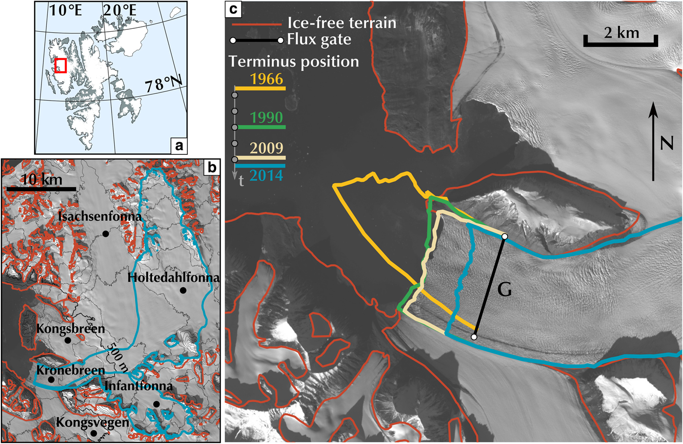
Fig. 1. (a) Study area on the west coast of the Svalbard archipelago. (b) Extent of Kronebreen, Infantfonna and Holtedahlfonna (blue line). Ice-free terrains are outlined in red. KRB is limited in the north by Kongsbreen and Isachsenfonna. It is joined 4 km before the terminus by Kongsvegen. (c) The terminus area. KRB terminus position for 1966 (yellow), 1990 (green), 2009 (beige) and KRB extent in 2014 (blue) are shown. The black line (G) shows the position of the flux gate used for the flux calculation. Background image is a SPOT5 image from 2007 (copyright CNES 2007, Distribution Airbus D&S, Korona and others, Reference Korona, Berthier, Bernard, Rémy and Thouvenot2009).
3. DATA
3.1. Geodetic volume change
Four Pléiades stereo pairs were acquired between 9 (two pairs), 16 and 25 August 2014 (Fig. 2). The panchromatic images have a resolution of 0.7 m at nadir. None of these acquisitions exhibited image saturation, a result of the 12-bit encoding and the low sun angle at the time of acquisition (Berthier and others, Reference Berthier2014). Four DEMs were calculated with the Ames Stereo Pipeline (Willis and others, Reference Willis, Herried, Bevis and Bell2015; Shean and others, Reference Shean2016) and merged in a single DEM mosaic after co-registration on their overlapping areas. The DEM of 16 August 2014 is arbitrarily chosen as a reference to which the other DEMs are 3-D co-registered following the method proposed in Nuth and Kääb (Reference Nuth and Kääb2011). Horizontal and vertical shifts of several metres are removed, which reduced the median and normalized median absolute deviation (NMAD, Höhle and Höhle, Reference Höhle and Höhle2009) of the elevation differences within the three overlapping areas to 1 m or less on the glacierized terrain (Table 1). An alternative DEM mosaic was created in which, after the 3-D co-registration, a correction of a tilt along the longitudinal and latitudinal axes was added. On steeper non-glacierized terrain, the spread of the elevation difference represented by the NMAD is up to 2.6 m, reflecting the sensitivity of DEM precision to surface slopes (Lacroix and others, Reference Lacroix, Berthier and Maquerhua2015). In their overlapping areas, we average the elevations of all available DEMs to ensure a seamless mosaic (Fig. 2).
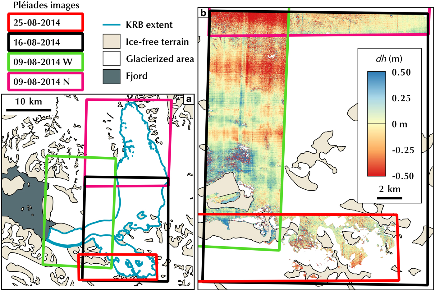
Fig. 2. (a) Extent of the different Pléiades scenes colour-coded with the date of the acquisition. (b) Elevation difference (in metres) between the different Pléiades DEMs over their overlapping areas.
Table 1. Shift vector removed by co-registration between Pléiades DEMs of the 9 and 25 August 2014 and the reference 16 August 2014 DEM (Easting, Northing, Z)
Statistical metrics of the elevation difference (Median dh and NMAD dh) after co-registration in metres on the glacier and off the glacier (i.e. stable terrain) provide a measure of the uncertainty of the high-resolution satellite product. N dh is the number of points in the area qualified.
A 2009 DEM was generated from aerial images acquired on 1 August 2009 by the Norwegian Polar Institute (NPI). Images had a ground sampling distance of ~50 cm and an overlap of ~60% in the along-track direction. DEMs were generated using the software Socet GXP (https://www.geospatialexploitationproducts.com/content/socet-gxp/). The final DEM has a pixel spacing of 5 m and an estimated vertical precision of 1–2 m (Norwegian Polar Institute, Terrengmodell Svalbard, 2014).
The 1966 and 1990 DEMs were generated from aerial photographs in a similar way as above (Altena, Reference Altena2008). Lack of texture in the original images, in particular the ones from 1990, led to a limited coverage of the DEMs in the upper accumulation areas. A kinematic GPS profile from 1996 is used to help constrain upper elevations in the 1990 DEM (Nuth and others, Reference Nuth, Schuler, Kohler, Altena and Hagen2012). The 1966, 1990 and 2009 DEMs are referenced to mean sea level using a local geoid–ellipsoid conversion produced by NPI (personal communication from Harald Faste-Aas, 2016).
3.2. Climatic mass balance
The climatic mass balance between 1966 and 2014 is calculated using a coupled surface-energy-balance-snow model to simulate mass and energy exchange between the atmosphere, surface and underlying snow, firn and/or ice on a 100 m regularly spaced grid at a 3 h time resolution (Van Pelt and others, Reference Van Pelt2012; Van Pelt and Kohler, Reference Van Pelt and Kohler2015). The model solves the surface energy balance to calculate surface temperature and melt, and simulates the subsurface evolution of temperature, density and water content. The model is primarily driven by output from the regional climate model HIRLAM (Undén and others, Reference Undén2002; Reistad and others, Reference Reistad2011), complemented with weather station data from the Ny-Ålesund meteorological station, provided by the Norwegian Meteorological Institute. The model is calibrated by in situ surface mass-balance measurements from stakes along the centreline of KRB. A complete model description, including the model setup, calibration and validation for KRB and Kongsvegen, can be found in Van Pelt and Kohler (Reference Van Pelt and Kohler2015).
3.3. Frontal ablation
Frontal ablation  $\dot{A}_{\rm f}$ is defined as the combined loss of calving icebergs, subaerial melt, subaerial sublimation and subaqueous frontal melting (Cogley and others, Reference Cogley2011). It can be measured by the sum of the discharge through the terminus position at the end of each studied period (1990, 2009 and 2014) and the mass change resulting from the advance or retreat of the terminus position during a period (e.g. Dunse and others, Reference Dunse2015). We estimate discharge through a single flux gate (Fig. 1) by combining a time series of surface velocity fields from 2009 to 2014 (Köhler and others, Reference Köhler2016) and measurements of glacier thickness from ground-penetrating radar (Lindbäck and others, Reference Lindbäck2018). From 2009 to 2013, 2 m resolution FORMOSAT-2 images were acquired at 2–5 weeks intervals while monoscopic Pléiades images (0.7 m resolution) were acquired at a roughly monthly interval between April and August 2014. Images were orthorectified using ground control points extracted from a 5 m 2007 SPOT5-HRS orthoimage and DEM (Korona and others, Reference Korona, Berthier, Bernard, Rémy and Thouvenot2009) and the 2014 Pléiades DEM produced for this study (details in Köhler and others, Reference Köhler2016). The bed elevation and the surface DEM at the beginning of a period are combined to calculate the volume changes due to changes in the terminus position.
3.4. Additional datasets
Glacier outlines are necessary to spatially integrate the components of the mass budget. Masks of the glacierized and non-glacierized terrains in each DEM are based on the multitemporal inventory derived from the original 1966, 1990 and 2007 DEMs (Nuth and others, Reference Nuth2013), and included in GLIMS (Raup and others, Reference Raup2007) and the Randolph Glacier inventory (Pfeffer and others, Reference Pfeffer2014). The glacier outlines are held constant in the accumulation area through the different time periods (i.e. ice divides are assumed stable) and only updated in the glacier terminus area where large changes occurred. Calving front positions were manually digitized from the DEMs or orthophotos. The KRB outline is well constrained by outcrops and nunataks, neighbouring glaciers and the fjord water at the front. Yet the exact location of the ice divide between KRB and Kongsbreen/Isachsenfonna remains uncertain. We test the sensitivity of our results to different locations of the ice divide (see Discussion).
4. METHODS
4.1. Mass-balance equation
The basic formulation of our mass budget approach is:
 $$\dot{M} = \dot{B} + \dot{A}_{\rm f},$$
where  $\dot{M}$ is the total glacier mass balance, $\dot{B}\; $ is the climatic mass balance (including surface and subsurface processes of internal accumulation and refreezing) and $\dot{A}_{\rm f}$ is the frontal ablation (including calving flux, melt and sublimation of the calving face). The overdot denotes derivative with respect to time and capital letters quantities summed for the entire glacier. We estimate KRB total mass balance with the geodetic method, $\; \dot{M}_{\rm g}$, and the mass budget method, $\dot{M}_{{\rm mb}}$. The geodetic method requires a conversion factor, ρ, to convert the total volume change, $\dot{V},$ into mass change (Eqn (2)). Note that ρ is not equivalent to material density in our method.
 $$\dot{M}_{\rm g} = \rho \times \dot{V}.$$
 The mass budget method relies on the calculation of the frontal ablation,  $\dot{A} $f and the climatic mass balance, $\dot{B}\; $:
 $$\dot{M}_{{\rm mb}} = \dot{B} + \dot{A}_{\rm f}{\rm.} $$
 Frontal ablation is the most difficult quantity to estimate as (i) the bed elevation or ice thickness is first required, and (ii) continuous velocity fields are needed, which is generally achieved only for more contemporary periods (post 2000). Therefore, Eqns (1) and (2) can be re-arranged to estimate frontal ablation as a residual, by the difference between the climatic mass balance ( $\dot{B}$) and the geodetic mass balance ( $\dot{M}_{\rm g}$):
 $$\dot{A}_{\rm f} = \dot{B}-\; \dot{M}_{\rm g}.$$
In this paper, we will distinguish between ‘measured’ and ‘estimated’ values. The former are directly derived from observations and from the model, whereas the latter are estimated from the residual of the mass continuity equation (Eqn (4)). All the terms of the mass-balance equation can be independently calculated for the period 2009–2014. These independent approaches are used to test our ability to close the mass budget. If not specified, mass-balance components are expressed as specific mass balance, which means a rate of change per surface unit. Additionally, we estimate emergence velocities for each elevation bin of the glacier from the residual of the observed elevation change and the modelled climatic elevation change. Upward velocities are taken as positive.
4.2. Geodetic mass balance
The geodetic mass balance is the sum of the mass change by change in the terminus position,  $\dot{q}_{\rm t}$, and by surface elevation changes over the glacierized area, $\dot{M}_{{\rm gla}}$. These two components are measured, respectively, by subtracting a surface DEM and the bedrock elevation over the retreated area (see Frontal ablation) and by subtracting two surface DEMs over glacier area. The 1966, 1990 and 2009 DEMs are first converted to WGS84 ellipsoidal heights. The 1966, 1990 and 2014 DEMs are then co-registered to the 2009 DEM using the ice-free terrain, which is unevenly distributed within the coverage of the combined DEMs. Co-registration performance is evaluated using the median and NMAD of the elevation differences on the ice-free terrain, ranging in absolute values from 0.02 m to 0.66 m and 0.84 m to 4.42 m, respectively, between two successive DEMs (Table 2).
Table 2. Shift vectors removed by co-registration between the DEMs and the reference 2009 NPI DEM
Statistics of the elevation difference map of the successive DEMs (1990−1966, 2009−1990, 1996−1990, 2014−2009). The normalized median absolute deviation (NMAD) and area are also provided. All metrics are in metres, except where stated. The 1996 GPS profile* was vertically adjusted to the 1990 DEM, using 114 overlapping points between the profile and the DEM on the glacier.
Glacier volume change upstream of the terminus position at the end of a period is obtained from the elevation differences using a hypsometric approach, which overcomes the existence of small data gaps in maps of elevation differences. In this approach, the glacier is discretized into 50 m elevation bands (i) from which the mean of the differences,  $\overline {\dot{h}} _i$, are calculated after removing outliers larger than three times the NMAD around the median. The total glacier volume change is obtained by multiplying the $\overline {\dot{h}} _i$ with the area A i of each elevation bin and then summing through all the elevation bands:
 $$\dot{V} = \; \mathop \sum \limits_i^{} \overline {\dot{h}} _i\; \times \; A_i.\; \; $$
The total volume of the glacier is calculated similarly by integrating elevation difference between a DEM and the bed elevation over the whole glacier. Elevation data are lacking in the 1990 DEM above 700 m a.s.l. and replaced by a differential GPS profile acquired along the centreline in 1996 with an accuracy of ~0.25 m. The profile is raised by a vertical shift of +3.69 m, the value identified in the 5 km of the 1996 profile that overlaps the 1990 DEM. This assumes that changes from 1990 to 1996 are uniform in the overlapping part, between 670 and 720 m a.s.l., and above.
Finally, the volume changes are converted into water equivalent mass change by multiplying by a volume change to mass change conversion factor ρ (Eqn (2)). Huss (Reference Huss2013) proposed using 850 ± 60 kg m−3 for land-terminating glaciers without significant frontal ablation. Here, we use a larger value of 900 ± 100 kg m−3 for the glacierized area as we believe that most KRB mass changes occur at higher density (see Discussion). We use the value of ice density for the volume change downstream the terminus position at the end of the period.
The volume change uncertainty  $e_{{\dot{V}}}$ results from error in the elevation difference map $e_{{\dot{h}}}$ as well as error in the glacier area e A:
 $$e_{\dot{V}} = \vert {\dot{V}} \vert \sqrt {{\left( {\displaystyle{{e_{{\dot{h}}}} \over {\dot{h}}}} \right)}^2 + {\left( {\displaystyle{{e_{\rm A}} \over A}} \right)}^2}. $$
 In Eqn (6), we use the statistics of the elevation difference map over ice-free terrain to estimate the random and systematic error in  $\dot{h}$. The systematic error is set to the median elevation difference, between 0.02 and 0.66 m (Table 2). We assume the systematic error to be a minimum of 0.5 m, based on the cyclic co-registration of three (or more) DEMs on the ice-free terrain. The sum of the co-registration vectors is non-zero due to the uncertainty of the co-registration method (Paul and others, Reference Paul2015). We set the random error to the NMAD of elevation difference over all ice-free terrain, between 0.84 and 4.42 m (Table 2). Random error is calculated assuming an autocorrelation distance of 1 km. The random error is several orders of magnitude lower than the systematic error, as the large glacier area, 368 km2 in 2014, ensures a sufficiently large number of independent points. The relative error of the glacier area, e A/A, is set to 7% after considering alternative likely glacier limits, in particular for uncertain ice divides (see Fig. 3b and Discussion).
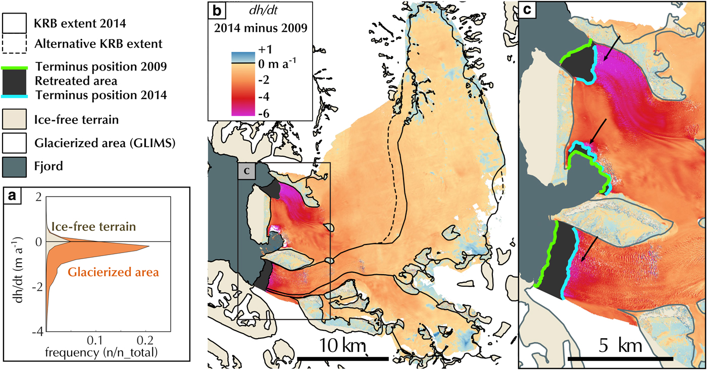
Fig. 3. Elevation difference between the 2009 and 2014 DEMs. (a) Distribution of elevation differences over ice-free terrain (filled beige) and glacierized terrain (filled orange). (b) Map of the elevation differences over the entire study area. Warm colours represent areas of elevation loss while blue colours represent the area of elevation gain. Dashed line represents the alternative mask used for sensitivity analysis. (c) Close-up of the terminus of KRB and Kongsbreen. Arrows point to zones of intense thinning.
The error of the geodetic mass balance  $e_{{{\dot{M}}}_{g}}$ is the root sum of squares of the error of the retreated mass, $e_{\dot{\rm q}_{\rm t}},$ and the mass change over the glacierized area, $e_{{{ \dot{M}}}_{{gla}}}$. For each, error accumulates from errors in the conversion factore ρ and the volume change rate $\; e_{{ \dot{V}}}$:
 $$e = \vert {\dot{M}} \vert \sqrt {{\left( {\displaystyle{{e_{{ \dot{V}}}} \over {\dot{V}}}} \right)}^2 + {\left( {\displaystyle{{e_\rho} \over \rho}} \right)}^2}. $$
We use the relative importance of the mass-balance equation terms and their density to determine the conversion factor uncertainty of ±100 kg m3 (see Discussion).
4.3. Frontal ablation
Frontal ablation,  $\dot{A}_{\rm f}$, is calculated from discharge through the terminus position at the end of a period, as the sum of ice discharge at the terminus $\dot{q}_{{\rm fg}}$, and mass loss due to terminus position change $\dot{q}_{\rm t}$ similarly to Schellenberger and others (Reference Schellenberger, Dunse, Kääb, Kohler and Reijmer2015):
 $$\dot{A}_{\rm f} = \dot{q}_{{\rm fg}} + \dot{q}_{\rm t}.$$
We calculate a continuous time series of discharge from 2009 to 2014 at a flux gate (G in Fig. 1), ~1 km above the August 2014 terminus position using 48 velocity fields u, and glacier thickness h:
 $$\dot{q}_{{\rm fg}} = \mathop \small \int \limits_G \!h \times u \times \rho _{{\rm ice}}.$$
Velocity fields of the glacier tongue are produced by standard image-matching techniques (COSI-CORR, Leprince and others, Reference Leprince, Barbot, Ayoub and Avouac2007; Heid and Kääb, Reference Heid and Kääb2012) on the high-resolution optical orthoimages from FORMOSAT-2 and Pléiades. G is selected to be as close as possible to the terminus and where the velocity fields are complete. Downstream of G, image matching is not possible due to iceberg calving. We extract velocities along the flux gate, convert to perpendicular flow and apply a small correction to the cross-section area by linearly interpolating the declining glacier surface elevation between the 2009 and 2014 DEMs. We assume constant speed from the glacier surface to the bedrock because basal sliding likely dominates near the terminus (Bahr, Reference Bahr2015). The discharge through the flux gate G is corrected for the climatic mass balance between the flux gate and the terminus to obtain the actual discharge at the terminus. For this purpose, we apply the modelled surface mass balance of the lowest elevation bin to the surface between the flux gate and the calving front position at the end of the period. Volume loss due to the terminus position change is obtained from the digitized terminus position, the bedrock and the glacier surface elevation at the beginning of the period. Again, a correction is applied, subtracting the climatic mass-balance contribution over the retreated area.
Error in discharge results from errors in the flux gate area, surface velocities and ice density assumption. The error in the flux gate area is a combination of the error of the bedrock elevation and the glacier surface elevation. A typical error for the bedrock is ~20 m (Lindbäck and others, Reference Lindbäck2018) which dominates the error of the DEMs (~5 m). We compare it to the average thickness at the front, ~140 m, and set the flux gate area error to 15%. The weekly to monthly surface velocity estimates are compared with continuous code-based GPS records at stakes over the same time periods (Schellenberger and others, Reference Schellenberger, Dunse, Kääb, Kohler and Reijmer2015). Results show a good agreement with a typical displacement difference of ~1.3 m which we conservatively assume as a systematic error leading to a 13 m a−1 error for the velocity (3% of the observed speed). We use the density of ice, 914 kg m−3, to convert volume flux into mass flux. High-resolution DEMs of KRB terminus show crevasses with a volume that is ~2–8% of the ice column from bedrock to the surface, justifying an error of 10% for the ice density.
4.4. Climatic mass balance
Output of the climatic mass-balance model is available at a 100 m spatial and 3 h temporal resolution (Van Pelt and Kohler, Reference Van Pelt and Kohler2015). The subsurface routine simulates temperature, density and water content evolution on a 50-layer vertical grid with layer depth increasing with distance to the surface. The climatic mass balance is calculated as the sum of precipitation, surface moisture exchange and runoff. Runoff either happens at the upper surface, in case of bare-ice exposure, or at the bottom of the firn/snowpack. The climatic mass balance hence accounts for mass fluxes related to refreezing and subsurface liquid water storage. Average climatic mass balance between dates of DEM collection is calculated by summing 3-hourly values. Glacier-wide climatic mass balances are calculated using a hypsometric approach (Eqn (5)) summed with the climatic mass balance over the retreated area. Additionally, model output of subsurface density profiles at dates of DEM collection are differenced to determine changes in firn column density through time.
The model error is estimated by comparing simulated values with in situ measurements at ablation/accumulation stakes. This centreline error assessment does not quantify potential errors due to spatial extrapolation to the whole glacier and the fact that the model is calibrated to the stake measurements. However, this indicates that the model does not have a systematic bias at the stake positions and that the temporal random error is ~0.25 m a−1 (Van Pelt and Kohler, Reference Van Pelt and Kohler2015). We combine the estimate of the model error e b with the area of the glacier error e A to obtain the total climatic mass-balance error. The error in the model results from the random error divided by the square root of the number of years, and assumes no systematic error:
 $$e_ {\dot {\rm B}} = \vert {\dot B} \vert \sqrt {{\left( {\displaystyle{{e_{\dot {\rm b}}} \over {\dot b}}} \right)}^2 + {\left( {\displaystyle{{e_{\rm A}} \over A}} \right)}^2}. $$
5. RESULTS
5.1. Closure of the 2009–2014 mass budget
For 2009–2014, we find a glacier-wide geodetic mass balance of −0.69 ± 0.12 m w.e. a−1 in which −0.20 ± 0.04 m w.e. a−1 derives from retreat of the terminus position. This estimate agrees, within the error limits, with the estimate using the mass budget method (−0.92 ± 0.16 m w.e. a−1), the sum of a slightly negative climatic mass balance at −0.14 ± 0.11 m w.e. a−1 and a strong frontal ablation at −0.78 ± 0.11 m w.e. a−1 (Fig. 4). The total mass loss, including terminus position change, can be partitioned into 15 ± 12% due to climatic mass balance and 85 ± 12% to frontal ablation, the latter of which comprises 22 ± 5% from retreat of the terminus position and 63 ± 11% from the discharge at the terminus (Table 3).
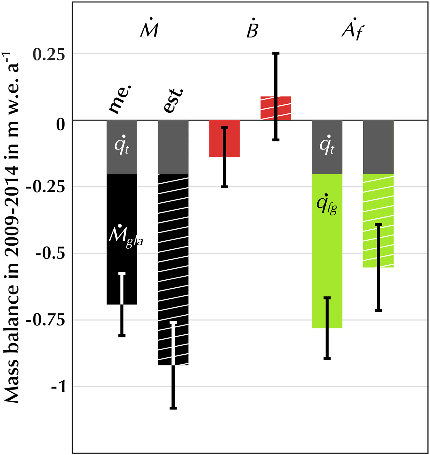
Fig. 4. Total mass balance from the geodetic method,  $\dot{M}\; {\rm me}{\rm.} $, from the mass budget method $\dot{M}\; {\rm est}{\rm.} $, and its component the climatic mass balance, $\dot{B}$, and the frontal ablation, $\dot{A}_{\rm f}$, for the validation period of 2009–2014 measured (flat bar) and estimated (hatched bar). The geodetic mass balance over glacierized area is in black, the climatic mass balance in red, the discharge at the terminus in green and the terminus position change contribution in grey. The mass loss by retreat of the terminus, $\dot{q}_{\rm t}$, is distinguished from the mass loss by discharge through the terminus, $\dot{q}_{{\rm fg}}$. The sum of the grey and green bars is the frontal ablation.
Table 3. The geodetic mass balance, climatic mass balance, discharge at the terminus and retreat mass are presented in m w.e. a−1
According to availability, the measured and/or the estimated value is shown.
The uncertainty in the geodetic mass balance includes uncertainties within the retreated area (13%) and in the glacierized area (87%). Over the 2014 glacierized area, the systematic error in the elevation difference map dominates (~62%), followed by the density conversion factor uncertainty (~18%) and the area uncertainty (~7%). We also calculated the geodetic mass balance with an alternative 2014 DEM in which the individual Pléiades DEMs were adjusted for tilts. In this case, geodetic mass balance is 6% less negative than the reference calculation (−0.65 ± 0.11 m w.e. a−1). This indicates the level of sensitivity to DEM co-registration and higher order biases. Climatic mass-balance error is dominated by the temporal random error (~99%).
5.2. Estimation of an unknown mass budget component
Based on the mass-balance equation (Eqn (1)), we successively consider the total mass balance, the frontal ablation and the climatic mass balance as unknown. Each estimated value is consistent with its measured counterpart within the error bars (Fig. 4), implying that we successfully closed the mass budget within the error limits for all variables. This validation is particularly valuable when estimating the climatic mass balance since the error of the model is harder to estimate than for observation-based components. The consistency of the estimated and measured climatic mass balance validates the model results and error estimate, but the short duration of the validation period (5 years) and the relatively small amount of refreezing within that period might limit the detection of a systematic model bias (see Discussion).
5.3. Geometry change and geodetic mass balance of KRB since 1966
KRB volume and area decreased during all three epochs, 1966–1990, 1990–2009 and 2009–2014. Glacier area variations are dominated by changes in the terminus position. Most area loss occurred during 1966–1990 and 2009–2014 with respective losses of 3.2 and 5.1 km2, while glacier area did not change significantly between 1990 and 2009. The cumulative loss from 1966 to 2014 is 9.1 km3, which represents ~10% of the total glacier volume in 1966 (86 ± 8 km3) (Lindbäck and others, Reference Lindbäck2018). Thinning is observed at all elevations (Fig. 5). Below 700 m a.s.l., the elevation change rate varied strongly between epochs with more loss during 1966–1990 and 2009–2014 than 1990–2009. Above 700 m a.s.l. elevation change was −0.40 ± 0.05 m a−1 in 1990–2009 and ~−0.10 ± 0.10 m a−1 in the other periods. The elevation difference map of 2009–2014 shows the surface elevation loss pattern in the lower part of KRB (Fig. 3). Only small patches in the higher parts of INF and HOD showed elevation increase. Figure 3c shows that surface lowering is greater upstream of retreating termini (KRB and northern branch of KNB) than stable ones (southern branch of KNB).
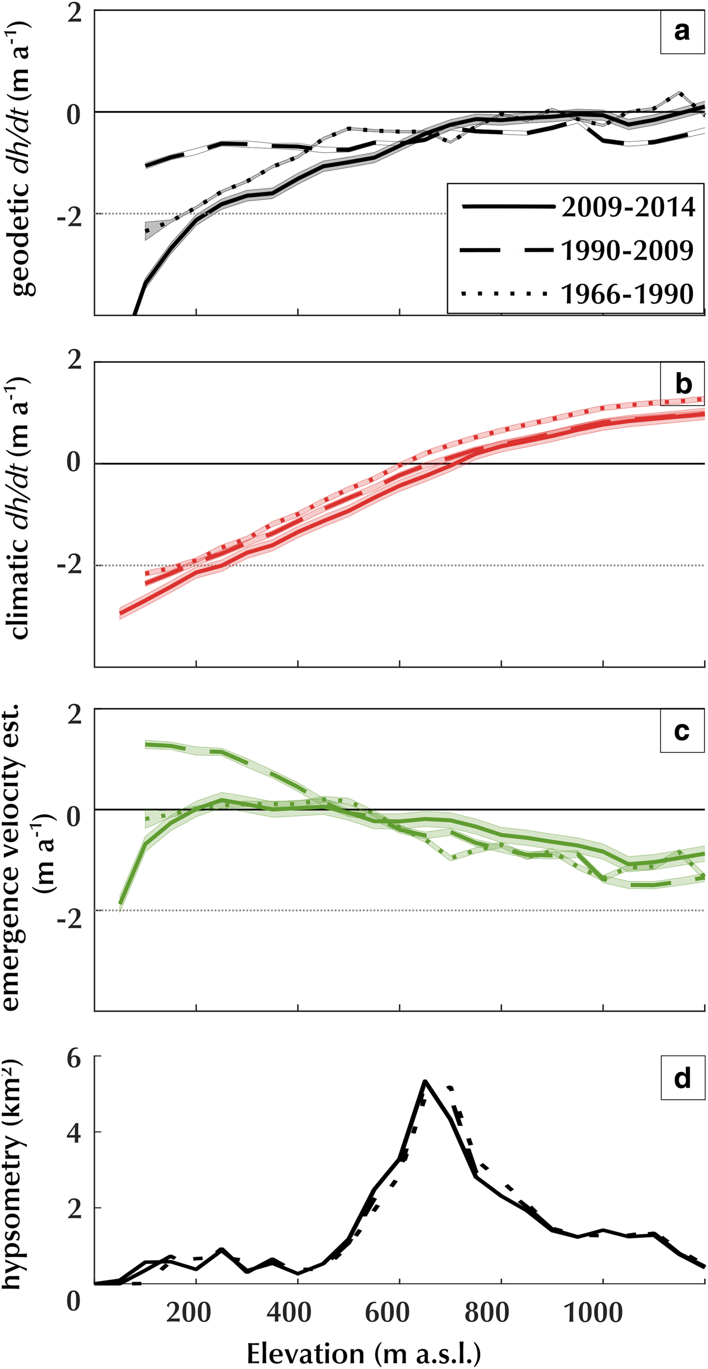
Fig. 5. Surface elevation changes, emergence velocity and hypsometry averaged in 100 m elevation bins. (a) Geodetic elevation change, (b) climatic elevation change, (c) emergence velocity deduced from the difference between (a) and (b). Line style indicates the epoch, dotted line for the 1966–1990 period, dashed line for 1990–2009 period and full line for the 2009–2014 period. Shaded area is the error. (d) Glacier hypsometry.
The geodetic mass balance of KRB is negative for all periods and has become increasingly so through time. For example, the large decrease from −0.46 ± 0.07 m w.e. a−1 for the period 1990–2009 to −0.69 ± 0.12 m w.e. a−1 for 2009–2014 is mainly the result of terminus position retreat between 2009 and 2014 (Table 3, Fig. 6). Excluding terminus position retreat, geodetic mass balance decreased most between 1966–1990 and 1990–2009, from −0.39 ± 0.05 to −0.46 ± 0.07 m w.e. a−1, and did not change significantly after. This decrease in geodetic mass balance (excluding terminus position retreat) is small and remains within the error limits.
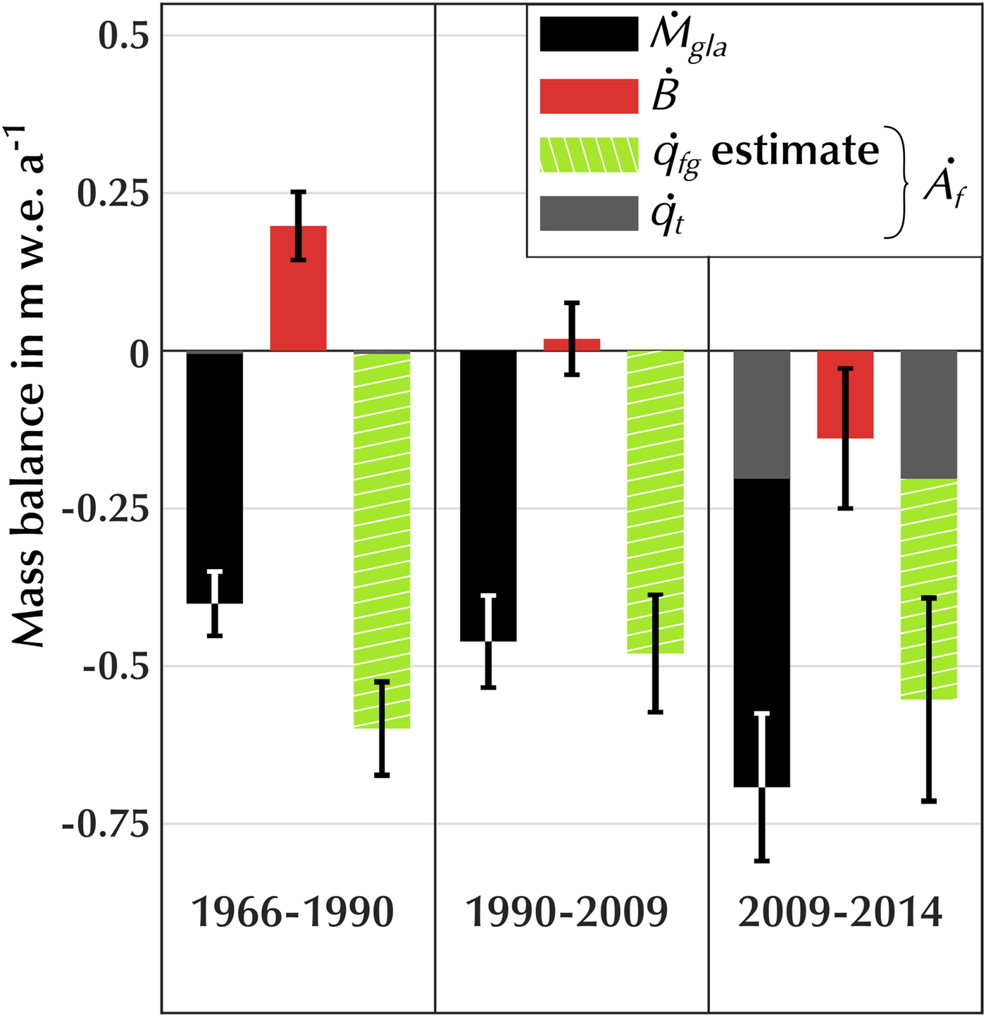
Fig. 6. Mass balance for three study periods measured with the geodetic method (black), separated between climatic mass balance (red), the estimated frontal ablation (green and grey). Grey shows the contribution of the terminus position retreat.
5.4. Climatic mass balance of KRB
Climatic mass balance decreased between every epoch from +0.20 ± 0.05 m w.e. a−1 for 1966–1990 to −0.14 ± 0.11 m w.e. a−1 for 2009–2014 (Table 3, Fig. 6). Locally, climatic mass balance for 1990–2009 was similar to the 1966–1990 period in the lowest part of the glacier but indicates more mass loss and less mass gain in every bin above 400 m a.s.l. The 2009–2014 period is uniformly more negative than the 1966–1990 period over all elevation bins by ~0.25 m a−1 (Fig. 5). The climatic equilibrium line altitude migrated up-glacier from ~600 m a.s.l. in 1966–1990 to ~700 m a.s.l. in 2009–2014 adding ~100 km2 to the ablation area (i.e. ~26% of the glacier total area in 1966). Consequently, the accumulation area ratio decreased from 59% in 1966–1990 to 34% in 2009–2014.
5.5. Frontal ablation of KRB
Frontal ablation is measured only for the 2009–2014 period and is estimated as a residual for all three periods. In 2009–2014, measured frontal ablation (−0.78 m w.e. a−1) is dominated by the discharge at the terminus (−0.58 m w.e. a−1) rather than retreat of the terminus position (−0.20 m w.e. a−1). The rate of mass loss due to the retreat of the terminus position varies from −0.01 ± 0 m w.e. a−1 for 1966–1990 to −0.20 ± 0.04 m w.e. a−1 for 2009–2014. The terminus position remained stable between 1990 and 2009. The retreat rate from 2009 to 2014 (5 years period) is one order of magnitude higher than in 1966–1990 (24 years period), which suggests that over long-time scales, discharge at the terminus dominates the frontal ablation. Estimated discharge at the terminus decreases in absolute value between 1996–1990 and 2009–2014 (Table 3, Fig. 6), although the magnitude of the decrease lies within the error bars.
5.6. Emergence velocities
Emergence velocities are negative (dynamic thinning) above a bed step at 500 m a.s.l. (Fig. 5), which corresponds also to the area where Holtedahlfonna narrows into Kronebreen tongue (Fig. 1). The elevation at which the emergence velocity becomes zero is stable through all three periods. Below this elevation, the emergence velocity is close to zero for 1966–1990 and 2009–2014. For 2009–2014, we observe negative emergence velocity below 200 m a.s.l., that is, in the last kilometre before the terminus. The period 1990–2009 shows clear positive emergence velocity below 500 m a.s.l.
6. DISCUSSION
6.1. Sensitivity tests
6.1.1. Sensitivity to uncertain glacier boundaries
The glacier boundaries are well defined at low elevations, as the contrast in satellite imagery is strong and the glacier is confined by mountains or moraines. Higher up, the dynamic division between KRB and Isachsenfonna is more uncertain, as no surface feature is visible, nor are surface flow measurement available. Placing the divide relies then on visual interpretation of satellite images. We repeated the mass budget calculations for an alternative mask which included an additional 26 km2 area between 500 and 1200 m a.s.l. (Fig. 3). The geodetic mass balance and climatic mass balance are modified by at most 0.01 m w.e. a−1. This small sensitivity is explained by the fact that the added area is around the climatic Equilibrium Line Altitude (ELA) (Fig. 3), a region where the elevation change is moderate and, by definition, the climate mass balance close to zero.
6.1.2. Density assumptions for geodetic mass balance
One potential source of error in estimating the geodetic mass balance (Eqn (2)) concerns conversion of the total volume change to total mass change which requires assumptions on material properties and the processes involved in the mass change. Ice melting or iceberg calving leads to mass loss of material at the ice density. Snowfall in the accumulation area leads after long enough time to a volume gain with ice density according to Sorge's law (Bader, Reference Bader1954). Over the short term, fresh snowfall, snow compaction and water refreezing can result in glacier volume change with densities different from ice density. The conversion factor is the average density of the volume added to and lost by the glacier. It is often taken to be at ice density or lower to account for mass change in the firn layer (Huss, Reference Huss2013). The conversion factor must therefore be adapted to individual glaciers’ settings and history. In Svalbard, internal refreezing of surface meltwater is common (Christianson and others, Reference Christianson, Kohler, Alley, Nuth and Van Pelt2015; Van Pelt and Kohler, Reference Van Pelt and Kohler2015) and results in conversion factor higher than ice density. Conversely, migration of the climatic ELA up-glacier exposes firn to melt, whose density is lower than ice. Using our data, we are able to compare the nature and the relative importance of the different mass-balance processes over KRB to constrain the conversion factor range.
KRB ice discharge at the terminus dominates the total mass balance during the three epochs (Table 3) with, for example, ice frontal ablation contributing to 85% of the total mass balance in 2009–2014. Therefore, during recent years, only 15% of the mass change depends on climatic mass-balance processes, whose conversion from volume to mass is most sensitive to the assumed density value. To assess the effect of variations in the conversion factor as a result of climatic mass-balance processes only, we calculate from the model runs the volume change to mass change conversion factor for the climatic mass balance for each pixel, i:
 $$\rho _i = \displaystyle{{{\dot{m}}_{i,{\rm CMB}}} \over {{\dot{h}}_{i,{\rm CMB}}}},$$
where  $\dot{m}_{i{\rm, CMB}}$ is the modelled mass change and $\dot{h}_{i{\rm, CMB}}$ the modelled elevation change. Below the ELA, the conversion factor is 0.9 since only ice melt occurs here over periods longer than a couple years. Above the ELA, an interesting pattern occurs, whereby the conversion factor is larger than the density of ice. The conversion factor in the accumulation area averages 1 020 kg m−3 in the period 1990–2009 and 980 kg m−3 in the period 2009–2014 (Fig. 7). This results from internal accumulation through which firn density increases combined with independent elevation change driven by snow accumulation. We stress that this conversion factor, purely derived from the model runs is relevant for the climatic mass balance only and is not to be used directly for the volume-to-mass change conversion of the geodetic method.
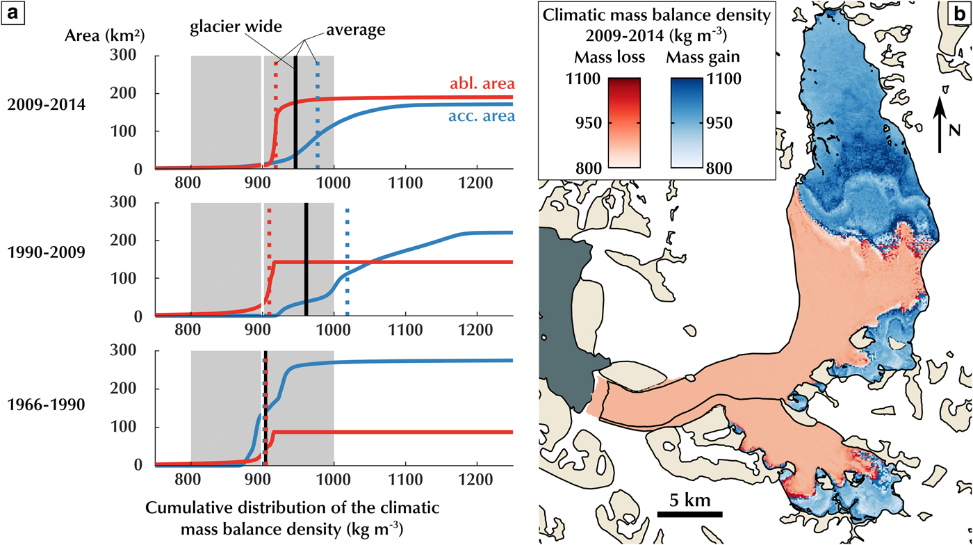
Fig. 7. Volume change to mass change conversion factor in the climatic mass-balance model. (a) Cumulative distribution of the density of the climatic mass loss (red line) and gain (blue line). Vertical line shows the average density of the climatic mass changes for the ablation area (dotted red), accumulation area (dotted blue) and the entire glacier (full black). Vertical white line shows the conversion factor used for calculation of the geodetic mass balance with error range (grey box). (b) Map of the density of the climatic mass change over KRB between 2009 and 2014. Blue shades show mass gain area, red shades show mass loss area.
6.2. Retrieving ice thickness and flux speed from the discharge
Bedrock elevation data are lacking for many tidewater glaciers. For the well-documented 2009–2014 period, we are able to estimate KRB thickness at the flux gate by using Eqns (4) and (9) and evaluate the results with the measured bedrock elevation (Lindbäck and others, Reference Lindbäck2018). During 2009–2014, the estimated flux through the flux gate is 0.13 ± 0.06 Gt a−1 which, using the observed gate-average speed (482 ± 10 m a−1), leads to an estimated average thickness of 93 ± 40 m. This is significantly smaller than the measured ice thickness of 157 ± 17 m. This indicates that reliable measurements of the ice thickness at a flux gate close to the tidewater glacier terminus remains necessary to retrieve reliable ice discharge and thus total mass balance using the mass budget method.
Similarly, we can estimate the average speed through the flux gate using the observed flux gate area to obtain a speed of 290 ± 130 m a−1 which underestimates significantly the measured speed of 482 ± 10 m a−1. If we assume that this bias is systematic, we can still interpret the evolution of the estimated average speed through the three epochs as the flux gate area is confidently measured at each date. We observe that the decrease of the glacier thickness at the flux gate does not explain completely the reduction of the estimated flux. A decrease in speed at the terminus is necessary. This slowdown would partially explain the general retreat of the terminus observed since 1966, so far explained by melting below sea level due to the ocean warming temperature (Luckman and others, Reference Luckman2015) and constrained by the bed topography (Lindbäck and others, Reference Lindbäck2018). However, sporadic measurements of glacier velocity exist from July 1964 to September 1965, May to September 1986 (Lefauconnier and others, Reference Lefauconnier, Hagen and Rudant1994) and July 1999 to July 2002 (Kääb and others, Reference Kääb, Lefauconnier and Melvold2005) but do not show any temporal trend. Velocities average over 1999–2002 is 435 m a−1 at a flux gate ~500 m downstream our flux gate (Kääb and others, Reference Kääb, Lefauconnier and Melvold2005) and is lower than our measurement for 2009–2014 (482 ± 10 m a−1). Comparison is hindered by the different position of the gates and the high year-to-year variability in KRB velocity close to the front (Luckman and others, Reference Luckman2015; Schellenberger and others, Reference Schellenberger, Dunse, Kääb, Kohler and Reijmer2015; Köhler and others, Reference Köhler2016). The significance of the lack of temporal trend is hard to determine as these sporadic measurements cover different time periods, especially given the very variable velocity of KRB through a year and from year to year (Köhler and others, Reference Köhler2016). Future work should investigate whether the LANDSAT, SPOT and ASTER archives can provide continuous measurements of frontal ablation back to 1990.
6.3. Comparison with similar studies
Our geodetic mass balances, excluding terminus position retreat, agree well with Nuth and others (Reference Nuth, Schuler, Kohler, Altena and Hagen2012) for 1966–1990 but differ for 1990–2007. Nuth and others (Reference Nuth, Schuler, Kohler, Altena and Hagen2012) estimate  $\dot{M}_{\rm g}$ = −0.68 ± 0.09 m a−1 while we found that $\dot{M}_{\rm g}$ = −0.46 ±0.07 m a−1 for 1990–2009. This difference in the geodetic calculation between the two studies remains unexplained. Climatic mass-balance values simulated in Nuth and others (Reference Nuth, Schuler, Kohler, Altena and Hagen2012) are systematically more negative by 0.20 m a−1 than those in this study (Van Pelt and Kohler, Reference Van Pelt and Kohler2015), which would result in larger residual in the mass budget. Accounting for internal accumulation through the sensitivity test in Nuth and others (Reference Nuth, Schuler, Kohler, Altena and Hagen2012) or the model physics (this study) results in better mass budget closure, suggesting the validity of integrating this phenomenon in the simulation. Nuth and others (Reference Nuth, Schuler, Kohler, Altena and Hagen2012) evaluated the scenario of having half of the melted water stored in the firn while the model used in this study explicitly calculates internal accumulation.
Our mass balance (excluding terminus position retreat) of −0.46 ± 0.07 m w.e. a−1 for 1990–2009 compares well with the mass balance over the northwest region of Svalbard based on ICESat laser altimetry, measured by Moholdt and others (Reference Moholdt, Nuth, Hagen and Kohler2010) to −0.54 ± 0.10 m a−1 for 2003–2009 or −0.49 ± 0.09 m w.e. a−1 using a conversion factor of 900 kg m−3, similar to our study. Our mass balance during 1966–2009 (−0.42 ± 0.08 m w.e. a−1) is also consistent with mass-balance measurement of land-terminating glaciers on the south coast of Kongsfjorden: Austre Brøggerbreen, Midtre Lovenbreen and Austre Lovenbreen, located, respectively, 17, 12 and 10 km east of KRB's terminus. James and others (Reference James2012) find a specific mass balance of −0.40 ± 0.03 m w.e. a−1 for Midtre Lovenbreen during 1966–2005 and −0.58 ± 0.03 m w.e. a−1 for Austre Brøggerbreen for 1966–2005, still using our conversion factor. Marlin and others (Reference Marlin2017) find a specific mass balance for 1962–2013 for Austre Lovenbreen of −0.44 ± 0.06 m w.e. a−1. Both studies observe an acceleration in the mass loss between the period before and after 1990 (James and others, Reference James2012) and 1995 (Marlin and others, Reference Marlin2017) by ~0.20 m w.e. a−1 due to more negative climatic mass balance. Kohler and others (Reference Kohler2007) report a similar acceleration in the mass loss of Midtre Lovenbreen. We observe a decrease in climatic mass balance of similar amplitude between 1966–1990 and 1990–2009 on KRB. However, we observe a different trend in the KRB geodetic mass balance, as variations in the frontal ablation add to the decrease in climatic mass balance. KRB experiences a fairly negative total mass balance compared with Austre Brøggerbreen, Midtre Lovenbreen and Austre Lovenbreen, despite its higher elevation; this can be primarily explained by the significant discharge at its front. We speculate that fluctuation in ice discharge might result from the cycle of damming and release of KRB's flow due to Kongsvegen's surge and retreat (Kääb and others, Reference Kääb, Lefauconnier and Melvold2005).
6.4. Emergence velocities
The stability of the elevation at which the emergence velocity becomes zero, despite changes downstream of it, suggests that its position is controlled by the shape of the glacier narrowing from a large accumulation zone to a valley glacier (Fig. 5). The fact that it is systematically below the climatic equilibrium line indicates an imbalance between the dynamics of KRB and its climatic conditions. Below this elevation we observe variations in emergence velocities synchronous with the unstable periods of the terminus. There, the emergence velocity is close to zero for 1966–1990 and 2009–2014, at a time when the terminus was retreating, indicating constant flux in time in this area. Conversely, the period of terminus stability 1990–2009 shows clear positive emergence velocity below 500 m a.s.l., indicating dynamical thickening. The negative emergence velocity close to the terminus in 2009–2014 is a sign of dynamic thinning, similar to observations in Novaya Zemlya (Melkonian and others, Reference Melkonian, Willis, Pritchard and Stewart2016). This illustrates the propagation of perturbations initiated at the terminus of tidewater glaciers which can lead to unstable retreat and impact upstream flow (Nick and others, Reference Nick, Vieli, Howat and Joughin2009). However, our frontal ablation estimations show no significant increase in discharge at the terminus despite the general terminus retreat trend. This suggests that the discharge is more constrained by the flux from upstream rather than the terminus position and stability.
6.5. Closing a tidewater glacier mass-balance budget
Closing a mass budget relies on the absolute value of the mass budget components and on the associated error. With sufficiently large error bars, it would always be possible to close the mass budget. We tried to calculate as carefully as possible each component and evaluate as honestly as possible their errors. However, the closing of the mass budget for KRB is relative as we close within error bars but error bars of estimated values do not overlap the measured value. This can arise from erroneous assumptions in our equations or error estimates. The error associated with the ice flux and the elevation change are validated against independent datasets or over ice-free terrain. The errors on the climatic mass balance are calculated using in situ stake measurements also used to calibrate the model. This might lead to erroneous estimation of the model error either through: (i) the lack of representativity of the stakes climatic mass balance due to spatially variable processes such as wind redistribution, or (ii) poor estimation of internal accumulation processes. These potential biases would accumulate over the studied periods. These errors are hard to detect from stake measurements, which can only indicate local mass changes above the last summer surface. Therefore, a systematic bias in the model cannot be completely disregarded as it would be hard to detect such a bias over a short 5-year period. A longer study period with similar datasets could help to confirm and quantify this possible bias.
7. SUMMARY AND CONCLUSIONS
We close the mass budget of the Kronebreen glacier system within our estimated errors for the period 2009–2014 by combining a unique dataset of satellite remote-sensing-based estimates of glacier volume changes and glacier frontal ablation with climatic mass-balance estimates from an energy-balance model constrained by in situ measurements. However, the closure of the budget is not strong as the errors of the estimated values do not overlap the measured values. Formal errors are largest for the remote-sensing-based estimates of glacier volume change and frontal ablation, rather than the mass-balance model. Retrieving the climatic mass balance from remote-sensing estimates of the geodetic mass balance and frontal ablation results in a positive value for 2009–2014, while the model suggests a negative value. The climatic mass-balance model performs well compared with KRB in situ data, but we are not yet able to rule out a potential systematic bias, for example, from small uncertainties in the parameters calibration or simply calibration from data along the centreline which does not account for accumulation or ablation transverse variability. The latter can induce small biases that accumulate through time. Nevertheless, our sensitivity test of estimating residuals in the mass budget equation from the 2009–2014 dataset allows us to justify the calculation of glacier frontal ablation or climatic mass balance as a residual during the earlier time periods (1966–2009) when observations (in situ or remote sensing) are lacking. The estimated frontal ablation is, however, too uncertain to recover the mean ice thickness or velocity at the terminus when only one of these two variables is known. The inherent errors in the various datasets do not allow us to accurately assess changes of mass balance between epochs; however, it seems likely that KRB geodetic mass balance, excluding terminus position change, remained stable between 1966 and 2014 despite increasingly negative climatic mass balance. This suggests that a decrease in frontal ablation compensated the climatic trend. Future studies with richer DEMs and more extended velocity fields may help constrain the temporality and the combination of processes which drive these phenomena.
ACKNOWLEDGEMENTS
We thank the two anonymous reviewers and Hester Jiskoot, the Scientific Editor, whose comments greatly improved this article. This work was supported by the French Space Agency (CNES), the Programme National de Télédétection Spatiale grant PNTS-2016-01, the Agence Nationale de la Recherche (ANR) Grant ANR-12-BS06-0018 (SUMER), the European Union/ERC (grant 320816) and the European Space Agency, Glaciers _CCI project (4000109873/14/I-NB).
AUTHORS CONTRIBUTION
C.N., E.B and C.D.B designed the study. E.B and C.D.B processed the Pléiades data. W.V.P produced the climatic mass-balance product and helped shape the study. C.N, J.K., E.B. and B.A. produced the flux data. B.A. produced the DEM from aerial photographs. C.D.B led the writing of the manuscript and all co-authors contributed to or commented on the manuscript.


 Open access